Elastic Registration of Medical Images With GANs

Abstract

Conventional approaches to image registration consist of time consuming iterative methods. Most current deep learning (DL) based registration methods extract deep features to use in an iterative setting. We propose an end-to-end DL method for registering multimodal images. Our approach uses generative adversarial networks (GANs) that eliminates the need for time consuming iterative methods, and directly generates the registered image with the deformation field. Appropriate constraints in the GAN cost function produce accurately registered images in less than a second. Experiments demonstrate their accuracy for multimodal retinal and cardiac MR image registration.

Index Terms—  GANs, deformable registration, displacement field

1 Introduction

Image registration is a fundamental step in most medical image analysis problems, and a comprehensive review of algorithms can be found in [1, 2, 3, 4, 5]. Conventional registration methods use iterative gradient descent based optimization using cost functions such as mean square error (MSE), normalized mutual information, etc. Such methods tend to be time consuming, especially for volumetric images. We propose a fully end-to-end deep learning (DL) approach that does not employ iterative methods, but uses generative adversarial networks (GANs) for obtaining registered images and the corresponding deformation field.

Thw works in [6, 7, 8, 9, 10] use convolutional stacked autoencoders (CAE) to extract features from fixed and moving images, and use it in a conventional iterative deformable registration framework. The works of [11, 12, 13, 14, 15, 16] use convolutional neural network (CNN) regressors in rigid registration of synthetic images. In [17, 18, 19, 20, 21] employ CNNs and reinforcement learning for iterative registration of CT to cone-beam CT in cardiac and abdominal images. DL based regression methods still require conventional methods to generate the transformed image.

Jaderberg et al. [22] introduced spatial transformer networks (STN) to align input images in a larger task-specific network. STNs, however, need many labeled training examples and have not been used for medical image analysis. Sokooti et. al. [23, 24, 25, 26, 27] propose RegNet that uses CNNs trained on simulated deformations to generate displacement vector fields for a pair of unimodal images. Vos et. al. [28, 29, 30, 31, 32, 33] propose the deformable image registration network (DIR-Net) which takes pairs of fixed and moving images as input, and outputs a transformed image non-iteratively. Training is completely unsupervised and unlike previous methods it is not trained with known registration transformations.

While RegNet and DIRNet are among the first methods to achieve registration in a single pass, they have some limitations such as: 1) using spatially corresponding patches to predict transformations. Finding corresponding patches is challenging in low contrast medical images and can adversely affect the registration task; 2) Multimodal registration is challenging with their approach due to the inherent problems of finding spatially corresponding patches; 3) DIRNet uses B-splines for spatial transformations which limits the extent of recovering a deformation field; 4) Use of intensity based cost functions limits the benefits that can be derived from a DL based image registration framework.

To overcome the above limitations we make the following contributions: 1) we use GANs for multimodal medical image registration, which can recover more complex range of deformations ; 2) novel constraints in the cost function, such as VGG, SSIM loss and deformation field reversibility, ensure that the trained network can easily generate images that are realistic with a plausible deformation field. We can choose any image as the reference image and registration is achieved in a single pass.

2 Methods

GANs are generative DL models trained to output many image types. Training is performed in an adversarial setting where a discriminator outputs a probability of the generated image matching the training data distribution. GANs have been used in various applications such as image super resolution [34, 35, 36, 37, 38, 39, 40], image synthesis and image translation using conditional GANs (cGANs) [41, 42, 43, 44, 45, 46] and cyclic GANs (cycGANs) [47, 48, 49, 50, 51, 52].

In cGANs the output is conditioned on the input image and a random noise vector, and requires training image pairs. On the other hand cycGANs do not require training image pairs but enforce consistency of deformation field. We leverage the advantage of both methods to register multimodal images. For multimodal registration we use cGANs to ensure the generated output image (i.e., the transformed floating image) has the same characteristic as the floating image (in terms of intensity distribution) while being similar to the reference image (of a different modality) in terms of landmark locations. This is achieved by incorporating appropriate terms in the loss function for image generation. Additionally, we enforce deformation consistency to obtain realistic deformation fields. This prevents unrealistic registrations and allows any image to be the reference or floating image. A new test image pair from modalities not part of the training set can be registered without the need for re-training the network.

2.1 Generating Registered Images

Let us denote the registered (or transformed) image as $I^{Trans}$, obtained from the input floating image $I^{Flt}$, and is to be registered to the fixed reference image $I^{Ref}$. For training we have pairs of multimodal images where the corresponding landmarks are perfectly aligned (e.g., retinal fundus and fluoroscein angiography (FA) images). Any one of the modalities (say fundus) is $I^{Ref}$. $I^{Flt}$ is generated by applying a known elastic deformation field to the other image modality (in this case FA). The goal of registration is to obtain $I^{Trans}$ from $I^{Flt}$ such that $I^{Trans}$ is aligned with $I^{Ref}$. Applying synthetic deformations allows us to: 1) accurately quantify the registration error in terms of deformation field recovery; and 2) determine the similarity between $I^{Trans}$ and FA images.

The generator network that outputs $I^{Trans}$ from $I^{Flt}$ is a feed-forward CNN whose parameters $\theta_{G}$ are,

$$\widehat{\theta}=\arg\min_{\theta_{G}}\frac{1}{N}\sum_{n=1}^{N}l^{SR}\left(G_{\theta_{G}}(I^{Flt}),I^{Ref},I^{Flt}\right),$$ (1)

where the loss function $l^{SR}$ combines content loss (to ensure that $I^{Trans}$ has desired characteristics) and adversarial loss, and $G_{\theta_{G}}(I^{Flt})=I^{Trans}$. The content loss is,

$$\begin{split}l_{content}&=NMI(I^{Trans},I^{Ref})+SSIM(I^{Trans},I^{Ref})\\ &+VGG(I^{Trans},I^{Ref}).\end{split}$$ (2)

$I^{Trans}$ should: 1) have identical intensity distribution as $I^{Flt}$ and; 2) have similar structural information content as $I^{Ref}$. $NMI(I^{Trans},I^{Ref})$ denotes the normalized mutual information (NMI) between $I^{Ref}$ and $I^{Trans}$. NMI is a widely used cost function for multimodal deformable registration [53, 54, 55, 56, 57, 58] since it matches the joint intensity distribution of two images. $SSIM(I^{Trans},I^{Ref})$ denotes the structural similarity index metric (SSIM) [59, 60, 61, 62, 63, 64] and calculates image similarity based on edge distribution and other landmarks. Since it is not based on intensity values it accurately quantifies landmark correspondence between different images. $VGG(I^{Trans},I^{Ref})$ is the $L2$ distance between two images using all $512$ feature maps of Relu $4-1$ layer of a pre-trained $VGG-16$ network [65, 66, 67, 68, 69, 70]. VGG loss improves robustness since the cost function takes into account multiple feature maps that capture information at different scales.

The adversarial loss of Eqn. 3 ensures that $I^{Trans}$ has an identical intensity distribution as $I^{Flt}$. We could realize this condition by having an extra $NMI(I^{Trans},I^{Flt})$ term in Eqn. 2. But this does not lead to much improvement in results.

The generator network $G$ (Figure 1(a)) employs residual blocks, each block having two convolutional layers with $3\times 3$ filters and $64$ feature maps, followed by batch normalization and ReLU activation. In addition to generating the registered image $G$ also outputs a deformation field. The discriminator $D$ (Figure 1 (b)) has eight convolutional layers with the kernels increasing by a factor of $2$ from $64$ to $512$ . Leaky ReLU is used and strided convolutions reduce the image dimension when the number of features is doubled. The resulting $512$ feature maps are followed by two dense layers and a final sigmoid activation to obtain a probability map. $D$ evaluates similarity of intensity distribution between $I^{Trans}$ and $I^{Ref}$, and the error between generated and reference deformation fields.

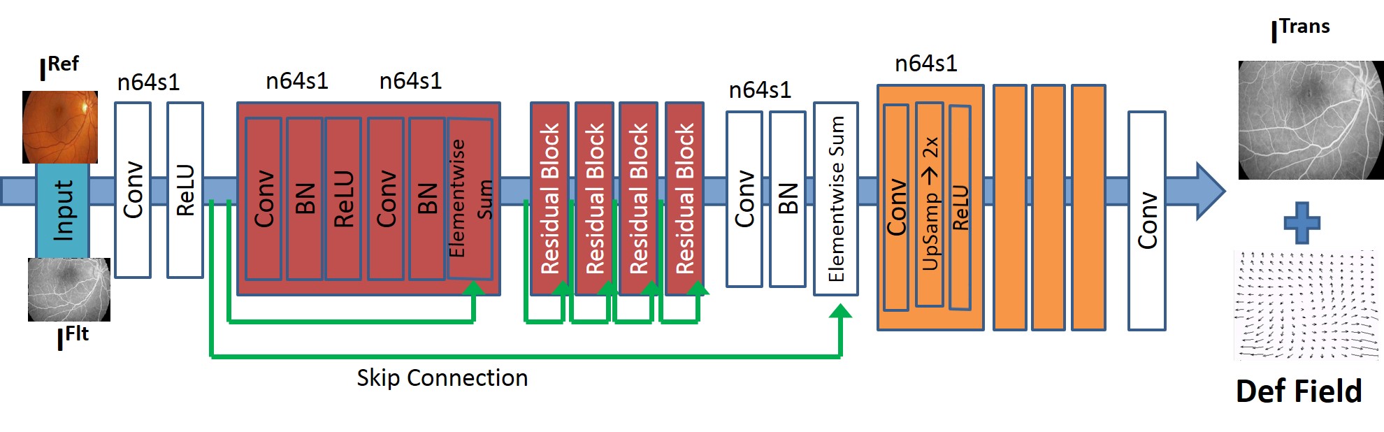
(a)

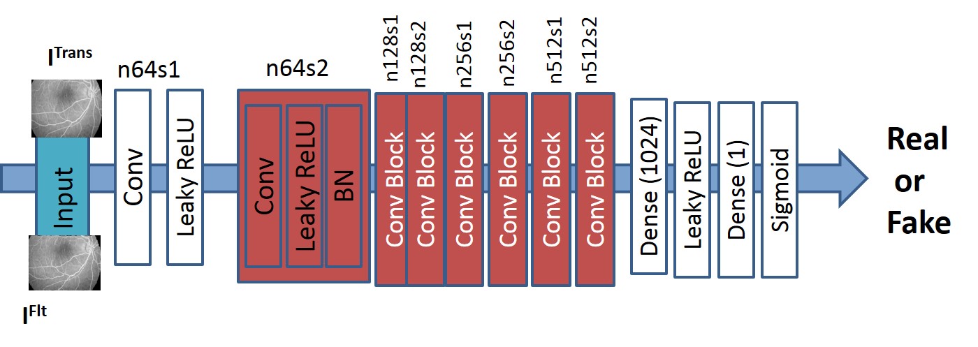
(b)

Fig. 1: (a) Generator Network; (b) Discriminator network. $n64s1$ denotes $64$ feature maps (n) and stride (s) $1$ for each convolutional layer.

2.2 Deformation Field Consistency

CycGANs learn mapping functions between two domains $X$ and $Y$ given training samples $x_{i=1}^{N}\in X$ and $y_{j=1}^{M}\in Y$. It has two transformations $G:X\rightarrow Y$ and $F:Y\rightarrow X$, and two adversarial discriminators $D_{X}$ and $D_{Y}$ , where $D_{X}$ differentiates between images ${x}$ and registered images ${F(y)}$ and $D_{Y}$ distinguishes between ${y}$ and ${G(x)}$. Here $X=I^{Flt}$ and $Y=I^{Ref}$. $G$ registers $I^{Flt}$ to $I^{Ref}$ while $F$ registers $I^{Ref}$ to $I^{Flt}$. In addition to the content loss (Eqn 2) we have: 1) an adversarial loss to match $I^{Trans}$’s distribution to $I^{Flt}$; and 2) a cycle consistency loss to ensure transformations $G,F$ do not contradict each other.

2.2.1 Adversarial Loss

The adversarial loss function for $G$ is given by:

$$\begin{split}&L_{cycGAN}(G,D_{Y},X,Y)=E_{y\in p_{data}(y)}\left[\log D_{Y}(y)\right]+\\ &E_{x\in p_{data}(x)}\left[\log\left(1-D_{Y}(G(x))\right)\right],\\ \end{split}$$ (3)

We retain notations $X,Y$ for conciseness. There also exists $L_{cycGAN}(F,D_{X},Y,X)$ the corresponding adversarial loss for $F$ and $D_{X}$.

2.2.2 Cycle Consistency Loss

A network may arbitrarily transform the input image to match the distribution of the target domain. Cycle consistency loss ensures that for each image $x\in X$ the reverse deformation should bring $x$ back to the original image, i.e. $x\rightarrow G(x)\rightarrow F(G(x))\approx x$. Similar constraints also apply for mapping $F$ and $y$. This is achieved using,

$$L_{cyc}(G,F)=E_{x}\left\|F(G(x))-x\right\|_{1}+E_{y}\left\|G(F(y))-y\right\|_{1},$$ (4)

The full objective function is

$$\begin{split}&L(G,F,D_{I^{Flt}},D_{I^{Ref}})=L_{cycGAN}(G,D_{I^{Ref}},I^{Flt},I^{Ref})\\ &+L_{cycGAN}(F,D_{I^{Flt}},I^{Ref},I^{Flt})+\lambda L_{cyc}(G,F)\end{split}$$ (5)

where $\lambda=10$ controls the contribution of the two objectives. The optimal parameters are given by:

$$G^{*},F^{*}=\arg\min_{F,G}\max_{D_{I^{Flt}},D_{I^{Ref}}}L(G,F,D_{I^{Flt}},D_{I^{Ref}})$$ (6)

The above formulation ensures $I^{Trans}$ to be similar to $I^{Flt}$ and also match $I^{Ref}$. We do not need to explicitly condition $I^{Trans}$ on $I^{Ref}$ or $I^{Flt}$ as that is implicit in the cost function (Eqns 2,3), which allows any pair of multimodal images to be registered even if the modality was not part of the training set.

3 Experiments and Results

We demonstrate the effectiveness of our approach on retinal and cardiac images. Details on dataset and experimental set up are provided later. Our method was implemented with Python and TensorFlow (for GANs). For GAN optimization we use Adam [71, 72, 73, 74, 75, 76] with $\beta_{1}=0.93$ and batch normalization. The ResNet was trained with a learning rate of $0.001$ and $10^{5}$ update iterations. MSE based ResNet was used to initialize $G$. The final GAN was trained with $10^{5}$ update iterations at learning rate $10^{-3}$. Training and test was performed on a NVIDIA Tesla K$40$ GPU with $12$ GB RAM.

3.1 Retinal Image Registration Results

The data consists of retinal colour fundus images and fluorescein angiography (FA) images obtained from $30$ normal subjects. Both images are $576\times 720$ pixels and fovea centred [77]. Registration ground truth was developed using the Insight Toolkit (ITK). The Frangi vesselness[78, 79, 80, 81, 82, 83, 84] feature was utilised to find the vasculature, and the maps were aligned using sum of squared differences (SSD). Three out of $30$ images could not be aligned due to poor contrast and one FA image was missing, leaving us with a final set of $26$ registered pairs. We use the fundus images as $I^{Ref}$ and generate floating images from the FA images by simulating different deformations (using SimpleITK) such as rigid, affine and elastic deformations(maximum displacement of a pixel was $\pm 10$ mm. $1500$ sets of deformations were generated for each image pair giving a total of $39000$ image pairs.

Our algorithm’s performance was evaluated using average registration error ($Err_{Def}$) between the applied deformation field and the recovered deformation field. Before applying simulated deformation the mean Dice overlap of the vasculature between the fundus and FA images across all $26$ patients is $99.2$, which indicates highly accurate alignment. After simulating deformations the individual Dice overlap reduces considerably depending upon the extent of deformation. The Dice value after successful registration is expected to be higher than before registration. We also calculate the $95$ percentile Hausdorff Distance ($HD_{95}$) and the mean absolute surface distance (MAD) before and after registration. We calculate the mean square error (MSE) between the registered FA image and the original undeformed FA image to quantify their similarity. The intensity of both images was normalized to lie in $[0,1]$. Higher values of Dice and lower values of other metrics indicate better registration. The average training time for the augmented dataset of $39000$ images was $14$ hours.

Table 1 shows the registration performance for $GAN_{Reg}$, our proposed method, and compared with the following methods: $DIRNet$ - the CNN based registration method of [28]; $Elastix$ - an iterative NMI based registration method [85, 86, 87, 88, 89, 90, 91]; and $GAN_{Reg_{nCyc}}$ - $GAN_{Reg}$ without deformation consistency constraints. $GAN_{Reg}$ has the best performance across all metrics. Figure 2 shows registration results for retinal images. $GAN_{Reg}$ registers the images closest to the original and is able to recover most deformations to the blood vessels, followed by $DIRNet$, $GAN_{Reg-nCyc}$, and $Elastix$. It is obvious that deformation reversibility constraints significantly improve registration performance. Note that the fundus images are color while the FA images are grayscale. The reference image is a grayscale version of the fundus image.

		After Registration
	Bef.	$GAN$	DIRNet	Elastix	$GAN$
	Reg.	Reg	[28]	[85]	${}_{Reg_{nCyc}}$
Dice	0.843	0.946	0.911	0.874	0.887
$Err_{Def}$	14.3	5.7	7.3	12.1	9.1
$HD_{95}$	11.4	4.2	5.9	9.7	8.0
MAD	9.1	3.1	5.0	8.7	7.2
MSE	0.84	0.09	0.23	0.54	0.37
$Time$ (s)		0.7	0.9	15.1	0.7

Table 1: Comparative average performance of different methods before and after retinal image registration. $Time$ denotes time in seconds taken to register a test image pair.

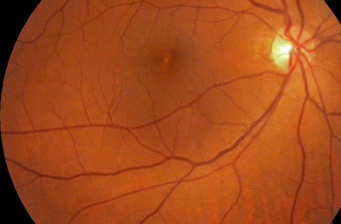
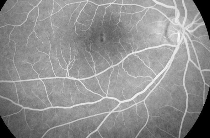
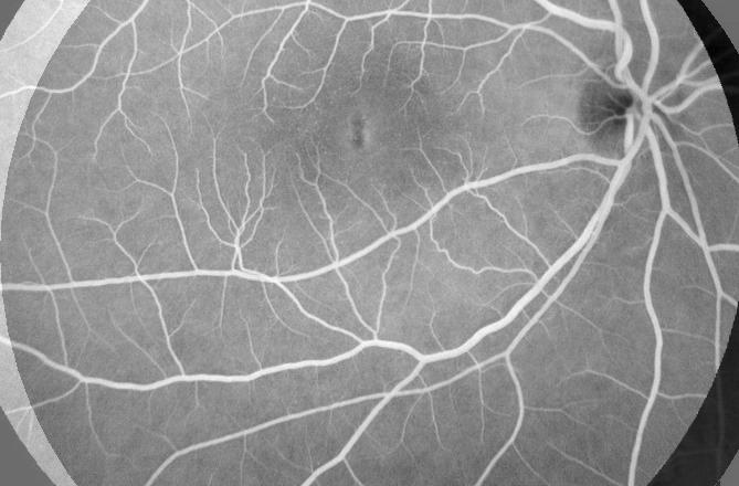
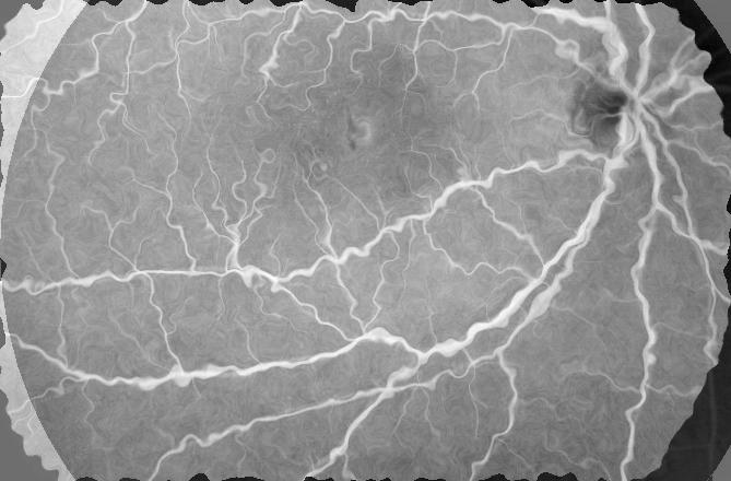
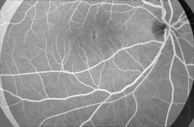
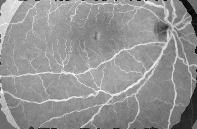
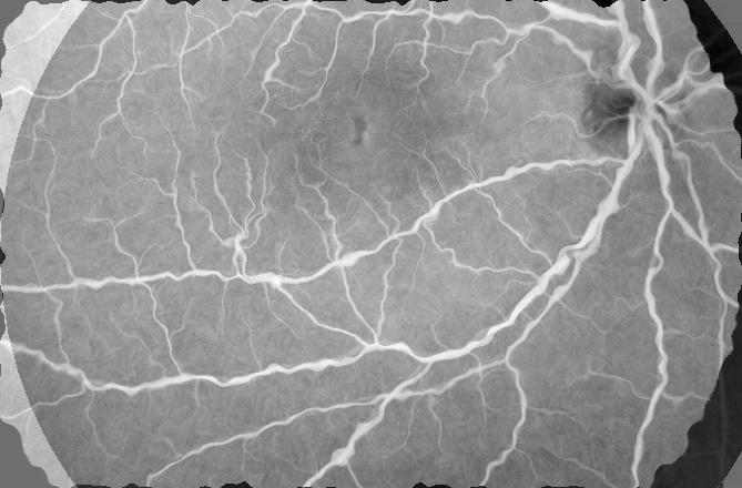
(a)	(b)	(c)	(d)	(e)	(f)	(g)	(h)

Fig. 2: Example results for retinal fundus and FA registration. (a) Color fundus image; (b) Original FA image; (c) ground truth difference image before simulated deformation; (d) Deformed FA image or the floating image; Difference image (e) before registration; after registration using (f) $GAN_{Reg}$; (g) $DIRNet$; (f) Elastix .

3.2 Cardiac Image Registration Results

The second dataset is the Sunybrook cardiac dataset [92] with $45$ cardiac cine MRI scans acquired on a single MRI-scanner. They consist of short-axis cardiac image slices each containing $20$ timepoints that encompass the entire cardiac cycle. Slice thickness and spacing is $8$ mm, and slice dimensions are $256\times 256$ with a pixel size of $1.28\times 1.28$ mm. The data is equally divided in $15$ training scans ($183$ slices), $15$ validation scans ($168$ slices), and $15$ test scans ($176$ slices). An expert annotated the right ventricle (RV) and left ventricle myocardium at end-diastolic (ED) and end-systolic (ES) time points. Annotations were made in the test scans and only used for final quantitative evaluation.

We calculate Dice values before and after registration, $HD_{95}$, and MAD. We do not simulate deformations on this dataset and hence do not calculate $Err_{Def},MSE$. Being a public dataset our results can be benchmarked against other methods. While the retinal dataset demonstrates our method’s performance for multimodal registration, the cardiac dataset highlights the performance in registering unimodal dynamic images. The network trained on retinal images was used for registering cardiac data without re-training. The first frame of the sequence was used as the reference image $I^{Ref}$ and all other images were floating images.

Table 2 summarizes the performance of different methods, and Figure 3 shows superimposed manual contour of the RV (red) and the deformed contour of the registered image (green). Better registration is reflected by closer alignment of the two contours. Once again it is obvious that $GAN_{Reg}$ has the best performance amongst all competing methods, and its advantages over $GAN_{Reg-nCyc}$ when including deformation consistency.

		After Registration
	Bef.	$GAN$	DIRNet	Elastix	$GAN$
	Reg.	Reg	[28]	[85]	${}_{Reg_{nCyc}}$
Dice	$0.62$	$0.85$	$0.80$	$0.77$	0.79
$HD_{95}$	$7.79$	$3.9$	$5.03$	$5.21$	5.12
MAD	$2.89$	$1.3$	$1.83$	$2.12$	1.98
$Time$ (s)		0.8	0.8	11.1	0.8

Table 2: Comparative average performance of different methods before and after cardiac image registration. $Time$ denotes time in seconds taken to register a test image pair..

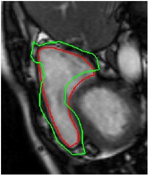
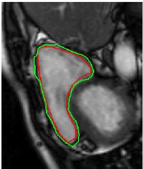
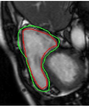
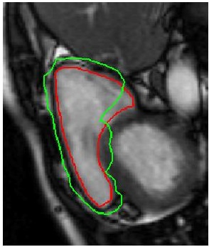
(a)	(b)	(c)	(d)

Fig. 3: Example results for cardiac RV registration. Superimposed contours of the ground truth (red) and deformed segmentation mask of moving image (green): (a) before registration; after registration using (b) $GAN_{Reg}$; (c) $DIRNet$; (d) Elastix.

4 Conclusion

We have proposed a GAN based method for multimodal medical image registration. Our proposed method allows fast and accurate registration and is independent of the choice of reference or floating image. Our primary contribution is in using GAN for medical image registration, and combining conditional and cyclic constraints to obtain realistic and smooth registration. Experimental results demonstrate that we perform better than traditional iterative registration methods and other DL based methods that use conventional transformation approaches such as B-splines.

References

- [1] M.A. Viergever, J.B.A Maintz, S. Klein, K. Murphy, M. Staring, and J.P.W. Pluim, “A survey of medical image registration,” Med. Imag. Anal, vol. 33, pp. 140–144, 2016.
- [2] B. Bozorgtabar, D. Mahapatra, H. von Teng, A. Pollinger, L. Ebner, J-P. Thiran, and M. Reyes, “Informative sample generation using class aware generative adversarial networks for classification of chest xrays.,” Computer Vision and Image Understanding, vol. 184, pp. 57–65, 2019.
- [3] D. Mahapatra, B. Bozorgtabar, and R. Garnavi, “Image super-resolution using progressive generative adversarial networks for medical image analysis.,” Computerized Medical Imaging and Graphics, vol. 71, pp. 30–39, 2019.
- [4] D. Mahapatra, “Semi-supervised learning and graph cuts for consensus based medical image segmentation.,” Pattern Recognition, vol. 63, no. 1, pp. 700–709, 2017.
- [5] J. Zilly, J.M. Buhmann, and D. Mahapatra, “Glaucoma detection using entropy sampling and ensemble learning for automatic optic cup and disc segmentation.,” In Press Computerized Medical Imaging and Graphics, vol. 55, no. 1, pp. 28–41, 2017.
- [6] G. Wu, M. Kim, Q. Wang, B. C. Munsell, , and D. Shen., “Scalable high performance image registration framework by unsupervised deep feature representations learning.,” IEEE Trans. Biomed. Engg., vol. 63, no. 7, pp. 1505–1516, 2016.
- [7] D. Mahapatra, F.M. Vos, and J.M. Buhmann, “Active learning based segmentation of crohns disease from abdominal mri.,” Computer Methods and Programs in Biomedicine, vol. 128, no. 1, pp. 75–85, 2016.
- [8] D. Mahapatra and J. Buhmann, “Visual saliency based active learning for prostate mri segmentation.,” SPIE Journal of Medical Imaging, vol. 3, no. 1, 2016.
- [9] D. Mahapatra, “Combining multiple expert annotations using semi-supervised learning and graph cuts for medical image segmentation.,” Computer Vision and Image Understanding, vol. 151, no. 1, pp. 114–123, 2016.
- [10] Z. Li, D. Mahapatra, J.Tielbeek, J. Stoker, L. van Vliet, and F.M. Vos, “Image registration based on autocorrelation of local structure.,” IEEE Trans. Med. Imaging, vol. 35, no. 1, pp. 63–75, 2016.
- [11] S. Miao, Y. Zheng Z.J. Wang, and R. Liao, “Real-time 2d/3d registration via cnn regression,” in IEEE ISBI, 2016, pp. 1430–1434.
- [12] D. Mahapatra, “Automatic cardiac segmentation using semantic information from random forests.,” J. Digit. Imaging., vol. 27, no. 6, pp. 794–804, 2014.
- [13] D. Mahapatra, S. Gilani, and M.K. Saini., “Coherency based spatio-temporal saliency detection for video object segmentation.,” IEEE Journal of Selected Topics in Signal Processing., vol. 8, no. 3, pp. 454–462, 2014.
- [14] D. Mahapatra and J.M. Buhmann, “Analyzing training information from random forests for improved image segmentation.,” IEEE Trans. Imag. Proc., vol. 23, no. 4, pp. 1504–1512, 2014.
- [15] D. Mahapatra and J.M. Buhmann, “Prostate mri segmentation using learned semantic knowledge and graph cuts.,” IEEE Trans. Biomed. Engg., vol. 61, no. 3, pp. 756–764, 2014.
- [16] D. Mahapatra, J.Tielbeek, J.C. Makanyanga, J. Stoker, S.A. Taylor, F.M. Vos, and J.M. Buhmann, “Automatic detection and segmentation of crohn’s disease tissues from abdominal mri.,” IEEE Trans. Med. Imaging, vol. 32, no. 12, pp. 1232–1248, 2013.
- [17] R. Liao, S. Miao, P. de Tournemire, S. Grbic, A. Kamen, T. Mansi, and D. Comaniciu, “An artificial agent for robust image registration,” in AAAI, 2017, pp. 4168–4175.
- [18] D. Mahapatra, J.Tielbeek, F.M. Vos, and J.M. Buhmann, “A supervised learning approach for crohn’s disease detection using higher order image statistics and a novel shape asymmetry measure.,” J. Digit. Imaging, vol. 26, no. 5, pp. 920–931, 2013.
- [19] D. Mahapatra, “Cardiac mri segmentation using mutual context information from left and right ventricle.,” J. Digit. Imaging, vol. 26, no. 5, pp. 898–908, 2013.
- [20] D. Mahapatra, “Cardiac image segmentation from cine cardiac mri using graph cuts and shape priors.,” J. Digit. Imaging, vol. 26, no. 4, pp. 721–730, 2013.
- [21] D. Mahapatra, “Joint segmentation and groupwise registration of cardiac perfusion images using temporal information.,” J. Digit. Imaging, vol. 26, no. 2, pp. 173–182, 2013.
- [22] M. Jaderberg, K. Simonyan, A. Zisserman, and K. Kavukcuoglu, “Spatial transformer networks,” in NIPS, 2015, pp. –.
- [23] H. Sokooti, B. de Vos, F. Berendsen, B.P.F. Lelieveldt, I. Isgum, and M. Staring, “Nonrigid image registration using multiscale 3d convolutional neural networks,” in MICCAI, 2017, pp. 232–239.
- [24] D. Mahapatra, “Skull stripping of neonatal brain mri: Using prior shape information with graphcuts.,” J. Digit. Imaging, vol. 25, no. 6, pp. 802–814, 2012.
- [25] D. Mahapatra and Y. Sun, “Integrating segmentation information for improved mrf-based elastic image registration.,” IEEE Trans. Imag. Proc., vol. 21, no. 1, pp. 170–183, 2012.
- [26] D. Mahapatra and Y. Sun, “Mrf based intensity invariant elastic registration of cardiac perfusion images using saliency information,” IEEE Trans. Biomed. Engg., vol. 58, no. 4, pp. 991–1000, 2011.
- [27] D. Mahapatra and Y. Sun, “Rigid registration of renal perfusion images using a neurobiology based visual saliency model,” EURASIP Journal on Image and Video Processing., pp. 1–16, 2010.
- [28] B. de Vos, F. Berendsen, M.A. Viergever, M. Staring, and I. Isgum, “End-to-end unsupervised deformable image registration with a convolutional neural network,” in arXiv preprint arXiv:1704.06065, 2017.
- [29] B. Bozorgtabar, M. Saeed Rad, D. Mahapatra, and J-P. Thiran, “Syndemo: Synergistic deep feature alignment for joint learning of depth and ego-motion,” in In Proc. IEEE ICCV, 2019.
- [30] Y. Xing, Z. Ge, R. Zeng, D. Mahapatra, J. Seah, M. Law, and T. Drummond, “Adversarial pulmonary pathology translation for pairwise chest x-ray data augmentation,” in In Proc. MICCAI, 2019.
- [31] D. Mahapatra and Z. Ge, “Training data independent image registration with gans using transfer learning and segmentation information,” in In Proc. IEEE ISBI, 2019, pp. 709–713.
- [32] D. Mahapatra, S. Bozorgtabar, J.-P. Thiran, and M. Reyes, “Efficient active learning for image classification and segmentation using a sample selection and conditional generative adversarial network,” in In Proc. MICCAI (2), 2018, pp. 580–588.
- [33] D. Mahapatra, Z. Ge, S. Sedai, and R. Chakravorty., “Joint registration and segmentation of xray images using generative adversarial networks,” in In Proc. MICCAI-MLMI, 2018, pp. 73–80.
- [34] C. Ledig and et. al., “Photo-realistic single image super-resolution using a generative adversarial network,” CoRR, vol. abs/1609.04802, 2016.
- [35] D Mahapatra, B Bozorgtabar, S Hewavitharanage, and R Garnavi, “Image super resolution using generative adversarial networks and local saliency maps for retinal image analysis,” in MICCAI, 2017, pp. 382–390.
- [36] S. Sedai, D. Mahapatra, B. Antony, and R. Garnavi, “Joint segmentation and uncertainty visualization of retinal layers in optical coherence tomography images using bayesian deep learning,” in In Proc. MICCAI-OMIA, 2018, pp. 219–227.
- [37] S. Sedai, D. Mahapatra, Z. Ge, R. Chakravorty, and R. Garnavi, “Deep multiscale convolutional feature learning for weakly supervised localization of chest pathologies in x-ray images,” in In Proc. MICCAI-MLMI, 2018, pp. 267–275.
- [38] D. Mahapatra, B. Antony, S. Sedai, and R. Garnavi, “Deformable medical image registration using generative adversarial networks,” in In Proc. IEEE ISBI, 2018, pp. 1449–1453.
- [39] S. Sedai, D. Mahapatra, S. Hewavitharanage, S. Maetschke, and R. Garnavi, “Semi-supervised segmentation of optic cup in retinal fundus images using variational autoencoder,,” in In Proc. MICCAI, 2017, pp. 75–82.
- [40] D. Mahapatra, S. Bozorgtabar, S. Hewavitahranage, and R. Garnavi, “Image super resolution using generative adversarial networks and local saliencymaps for retinal image analysis,,” in In Proc. MICCAI, 2017, pp. 382–390.
- [41] P. Isola, J.Y. Zhu, T. Zhou, and A.A. Efros, “Image-to-image translation with conditional adversarial networks,” in CVPR, 2017.
- [42] P. Roy, R. Tennakoon, K. Cao, S. Sedai, D. Mahapatra, S. Maetschke, and R. Garnavi, “A novel hybrid approach for severity assessment of diabetic retinopathy in colour fundus images,,” in In Proc. IEEE ISBI, 2017, pp. 1078–1082.
- [43] P. Roy, R. Chakravorty, S. Sedai, D. Mahapatra, and R. Garnavi, “Automatic eye type detection in retinal fundus image using fusion of transfer learning and anatomical features,” in In Proc. DICTA, 2016, pp. 1–7.
- [44] R. Tennakoon, D. Mahapatra, P. Roy, S. Sedai, and R. Garnavi, “Image quality classification for dr screening using convolutional neural networks,” in In Proc. MICCAI-OMIA, 2016, pp. 113–120.
- [45] S. Sedai, P.K. Roy, D. Mahapatra, and R. Garnavi, “Segmentation of optic disc and optic cup in retinal images using coupled shape regression,” in In Proc. MICCAI-OMIA, 2016, pp. 1–8.
- [46] D. Mahapatra, P.K. Roy, S. Sedai, and R. Garnavi, “Retinal image quality classification using saliency maps and cnns,” in In Proc. MICCAI-MLMI, 2016, pp. 172–179.
- [47] J.Y. Zhu, T.park, P. Isola, and A.A. Efros, “Unpaired image-to-image translation using cycle-consistent adversarial networks,” in arXiv preprint arXiv:1703.10593, 2017.
- [48] S. Sedai, P.K. Roy, D. Mahapatra, and R. Garnavi, “Segmentation of optic disc and optic cup in retinal fundus images using shape regression,” in In Proc. EMBC, 2016, pp. 3260–3264.
- [49] D. Mahapatra, P.K. Roy, S. Sedai, and R. Garnavi, “A cnn based neurobiology inspired approach for retinal image quality assessment,” in In Proc. EMBC, 2016, pp. 1304–1307.
- [50] J. Zilly, J. Buhmann, and D. Mahapatra, “Boosting convolutional filters with entropy sampling for optic cup and disc image segmentation from fundus images,” in In Proc. MLMI, 2015, pp. 136–143.
- [51] D. Mahapatra and J. Buhmann, “Visual saliency based active learning for prostate mri segmentation,” in In Proc. MLMI, 2015, pp. 9–16.
- [52] D. Mahapatra and J. Buhmann, “Obtaining consensus annotations for retinal image segmentation using random forest and graph cuts,” in In Proc. OMIA, 2015, pp. 41–48.
- [53] D. Rueckert, L.I Sonoda, C. Hayes, D.L.G Hill, M.O Leach, and D.J Hawkes., “Nonrigid registration using free-form deformations: application to breast mr images.,” IEEE Trans. Med. Imag.., vol. 18, no. 8, pp. 712–721, 1999.
- [54] D. Mahapatra and J.M. Buhmann, “A field of experts model for optic cup and disc segmentation from retinal fundus images,” in In Proc. IEEE ISBI, 2015, pp. 218–221.
- [55] D. Mahapatra, Z. Li, F.M. Vos, and J.M. Buhmann, “Joint segmentation and groupwise registration of cardiac dce mri using sparse data representations,” in In Proc. IEEE ISBI, 2015, pp. 1312–1315.
- [56] D. Mahapatra, F.M. Vos, and J.M. Buhmann, “Crohn’s disease segmentation from mri using learned image priors,” in In Proc. IEEE ISBI, 2015, pp. 625–628.
- [57] H. Kuang, B. Guthier, M. Saini, D. Mahapatra, and A. El Saddik, “A real-time smart assistant for video surveillance through handheld devices.,” in In Proc: ACM Intl. Conf. Multimedia, 2014, pp. 917–920.
- [58] D. Mahapatra, J.Tielbeek, J.C. Makanyanga, J. Stoker, S.A. Taylor, F.M. Vos, and J.M. Buhmann, “Combining multiple expert annotations using semi-supervised learning and graph cuts for crohn s disease segmentation,” in In Proc: MICCAI-ABD, 2014.
- [59] Z. Wang and et. al., “Image quality assessment: from error visibility to structural similarity.,” IEEE Trans. Imag. Proc., vol. 13, no. 4, pp. 600–612, 2004.
- [60] P. Schffler, D. Mahapatra, J. Tielbeek, F.M. Vos, J. Makanyanga, D.A. Pends, C.Y. Nio, J. Stoker, S.A. Taylor, and J.M. Buhmann, “Semi automatic crohns disease severity assessment on mr imaging,” in In Proc: MICCAI-ABD, 2014.
- [61] D. Mahapatra, J.Tielbeek, J.C. Makanyanga, J. Stoker, S.A. Taylor, F.M. Vos, and J.M. Buhmann, “Active learning based segmentation of crohn’s disease using principles of visual saliency,” in Proc. IEEE ISBI, 2014, pp. 226–229.
- [62] D. Mahapatra, P. Schffler, J. Tielbeek, F.M. Vos, and J.M. Buhmann, “Semi-supervised and active learning for automatic segmentation of crohn’s disease,” in Proc. MICCAI, Part 2, 2013, pp. 214–221.
- [63] P. Schffler, D. Mahapatra, J. Tielbeek, F.M. Vos, J. Makanyanga, D.A. Pends, C.Y. Nio, J. Stoker, S.A. Taylor, and J.M. Buhmann, “A model development pipeline for crohns disease severity assessment from magnetic resonance images,” in In Proc: MICCAI-ABD, 2013.
- [64] D. Mahapatra, “Graph cut based automatic prostate segmentation using learned semantic information,” in Proc. IEEE ISBI, 2013, pp. 1304–1307.
- [65] K. Simonyan and A. Zisserman., “Very deep convolutional networks for large-scale image recognition,” CoRR, vol. abs/1409.1556, 2014.
- [66] D. Mahapatra and J.M. Buhmann, “Automatic cardiac rv segmentation using semantic information with graph cuts,” in Proc. IEEE ISBI, 2013, pp. 1094–1097.
- [67] D. Mahapatra, J. Tielbeek, F.M. Vos, and J.M. Buhmann, “Weakly supervised semantic segmentation of crohn’s disease tissues from abdominal mri,” in Proc. IEEE ISBI, 2013, pp. 832–835.
- [68] D. Mahapatra, J. Tielbeek, F.M. Vos, and J.M. Buhmann ., “Crohn’s disease tissue segmentation from abdominal mri using semantic information and graph cuts,” in Proc. IEEE ISBI, 2013, pp. 358–361.
- [69] D. Mahapatra, J. Tielbeek, F.M. Vos, and J.M. Buhmann, “Localizing and segmenting crohn’s disease affected regions in abdominal mri using novel context features,” in Proc. SPIE Medical Imaging, 2013.
- [70] D. Mahapatra, J. Tielbeek, J.M. Buhmann, and F.M. Vos, “A supervised learning based approach to detect crohn’s disease in abdominal mr volumes,” in Proc. MICCAI workshop Computational and Clinical Applications in Abdominal Imaging(MICCAI-ABD), 2012, pp. 97–106.
- [71] D.P. Kingma and J. Ba, “Adam: A method for stochastic optimization,” in arXiv preprint arXiv:1412.6980,, 2014.
- [72] D. Mahapatra, “Cardiac lv and rv segmentation using mutual context information,” in Proc. MICCAI-MLMI, 2012, pp. 201–209.
- [73] D. Mahapatra, “Landmark detection in cardiac mri using learned local image statistics,” in Proc. MICCAI-Statistical Atlases and Computational Models of the Heart. Imaging and Modelling Challenges (STACOM), 2012, pp. 115–124.
- [74] F. M. Vos, J. Tielbeek, R. Naziroglu, Z. Li, P. Schffler, D. Mahapatra, Alexander Wiebel, C. Lavini, J. Buhmann, H. Hege, J. Stoker, and L. van Vliet, “Computational modeling for assessment of IBD: to be or not to be?,” in Proc. IEEE EMBC, 2012, pp. 3974–3977.
- [75] D. Mahapatra, “Groupwise registration of dynamic cardiac perfusion images using temporal information and segmentation information,” in In Proc: SPIE Medical Imaging, 2012.
- [76] D. Mahapatra, “Neonatal brain mri skull stripping using graph cuts and shape priors,” in In Proc: MICCAI workshop on Image Analysis of Human Brain Development (IAHBD), 2011.
- [77] S.A.M Hajeb, H. Rabbani, and M.R. Akhlaghi., “Diabetic retinopathy grading by digital curvelet transform.,” Comput Math Methods Med., pp. 7619–01, 2012.
- [78] A.F. Frangi, W.J. Niessen, K.L. Vincken, and M.A. Viergever, “Multiscale vessel enhancement filtering,” in MICCAI, 1998, pp. 130–137.
- [79] D. Mahapatra and Y. Sun, “Orientation histograms as shape priors for left ventricle segmentation using graph cuts,” in In Proc: MICCAI, 2011, pp. 420–427.
- [80] D. Mahapatra and Y. Sun, “Joint registration and segmentation of dynamic cardiac perfusion images using mrfs.,” in Proc. MICCAI, 2010, pp. 493–501.
- [81] D. Mahapatra and Y. Sun., “An mrf framework for joint registration and segmentation of natural and perfusion images,” in Proc. IEEE ICIP, 2010, pp. 1709–1712.
- [82] D. Mahapatra and Y. Sun, “Retrieval of perfusion images using cosegmentation and shape context information,” in Proc. APSIPA Annual Summit and Conference (ASC), 2010.
- [83] D. Mahapatra and Y. Sun, “A saliency based mrf method for the joint registration and segmentation of dynamic renal mr images,” in Proc. ICDIP, 2010.
- [84] D. Mahapatra and Y. Sun, “Nonrigid registration of dynamic renal MR images using a saliency based MRF model,” in Proc. MICCAI, 2008, pp. 771–779.
- [85] S. Klein, M. Staring, K. Murphy, M.A. Viergever, and J.P.W. Pluim., “Elastix: a toolbox for intensity based medical image registration.,” IEEE Trans. Med. Imag.., vol. 29, no. 1, pp. 196–205, 2010.
- [86] D. Mahapatra and Y. Sun, “Registration of dynamic renal mr images using neurobiological model of saliency,” in Proc. ISBI, 2008, pp. 1119–1122.
- [87] D. Mahapatra, M.K. Saini, and Y. Sun, “Illumination invariant tracking in office environments using neurobiology-saliency based particle filter,” in IEEE ICME, 2008, pp. 953–956.
- [88] D. Mahapatra, S. Roy, and Y. Sun, “Retrieval of mr kidney images by incorporating spatial information in histogram of low level features,” in In 13th International Conference on Biomedical Engineering, 2008.
- [89] D. Mahapatra and Y. Sun, “Using saliency features for graphcut segmentation of perfusion kidney images,” in In 13th International Conference on Biomedical Engineering, 2008.
- [90] D. Mahapatra, S. Winkler, and S.C. Yen, “Motion saliency outweighs other low-level features while watching videos,” in SPIE HVEI., 2008, pp. 1–10.
- [91] D. Mahapatra, A. Routray, and C. Mishra, “An active snake model for classification of extreme emotions,” in IEEE International Conference on Industrial Technology (ICIT), 2006, pp. 2195–2199.
- [92] P. Radau, Y. Lu, K. Connelly, G. Paul, and et. al ., “valuation framework for algorithms segmenting short axis cardiac MRI,” in The MIDAS Journal-Cardiac MR Left Ventricle Segmentation Challenge, 2009.