Systematics of the HAL QCD Potential
at Low Energies in Lattice QCD

Abstract

The $\Xi\Xi$ interaction in the ¹S₀ channel is studied to examine the convergence of the derivative expansion of the non-local HAL QCD potential at the next-to-next-to-leading order (N²LO). We find that (i) the leading order potential from the N²LO analysis gives the scattering phase shifts accurately at low energies, (ii) the full N²LO potential gives only small correction to the phase shifts even at higher energies below the inelastic threshold, and (iii) the potential determined from the wall quark source at the leading order analysis agrees with the one at the N²LO analysis except at short distances, and thus, it gives correct phase shifts at low energies. We also study the possible systematic uncertainties in the HAL QCD potential such as the inelastic state contaminations and the finite volume artifact for the potential and find that they are well under control for this particular system.

I Introduction

In lattice QCD, two methods have been proposed so far to study the baryon-baryon interactions. One is the direct method Yamazaki:2015asa ; Wagman:2017tmp ; Berkowitz:2015eaa , where the energy spectrum on finite volume(s) is extracted from the temporal correlation of two baryons and is converted to the scattering phase shift and/or the binding energy in the infinite volume through the Lüscher’s finite volume formula Luscher:1985dn ; Luscher:1990ux . The other is the HAL QCD method Ishii:2006ec ; Aoki:2009ji ; HALQCD:2012aa ; Aoki:2012tk ; Aoki:2012bb , where the potential between baryons is first derived from the spatial correlations of two baryons, and it is used to calculate the observables through the Schrödinger-type equation in the infinite volume.

While both methods are supposed to give the same results in principle, previous numerical studies for two-nucleon ($NN$) systems show clear discrepancy: The direct method indicates that both dineutron (¹S${}_{0})$ and deuteron (³S₁) are bound for heavy pion masses ($m_{\pi}\geq 300$ MeV), while the HAL QCD method does not provide such bound states in both channels for heavy pion masses. This discrepancy was recently discussed in a series of papers Iritani:2016jie ; Iritani:2017rlk ; Aoki:2017byw ; Iritani:2018vfn , where it was pointed out that the effective two-particle energy as a function of the Euclidean time may significantly suffer from elastic scattering states of two nucleons. To elucidate such uncertainties, certain “normality checks” for the finite-volume spectrums were introduced Iritani:2016jie ; Iritani:2017rlk ; Aoki:2017byw ; Iritani:2018vfn .

The advantage of the time-dependent HAL QCD method HALQCD:2012aa over the direct method is that the former is free from the ground state saturation problem in principle, since the energy-independent potential controls both ground state and the elastic excited states simultaneously as long as the inelastic scatterings in the small Euclidean time are properly suppressed. In practice, there appear systematic uncertainties associated with the truncation of the derivative expansion for the non-local potential. Therefore, the main purpose of the present paper is to study the convergence of the derivative expansion, as well as other sources of systematic uncertainties such as the inelastic state contaminations and the distortion of the interaction under finite volume. We consider the $\Xi\Xi$ system in the ¹S₀ channel and perform the (2+1)-flavor lattice QCD calculation at $m_{\pi}=0.51$ GeV and $m_{K}=0.62$ GeV. Because of the large quark masses, the statistical errors in this case become relatively small, so that one can focus on the detailed analysis of the systematic errors. Also, this channel and the $NN$ system in the ¹S₀ channel belong to the same multiplet in the flavor SU(3) limit.

This paper is organized as follows. In Sec. II, we review the time-dependent HAL QCD method. In Sec. III, we present the lattice QCD results for the $\Xi\Xi$ interaction in the ¹S₀ channel at the next-to-next-to-leading order (N²LO) in the derivative expansion. The N²LO potential is extracted from a specific combination of the $\Xi\Xi$ correlations with different source operators. The systematic errors associated with the inelastic state contaminations and the distortion in the finite volume are also examined. In Sec. IV, we calculate the scattering phase shifts in this channel, and check the convergence of the derivative expansion in the HAL QCD method. In Sec. V, we demonstrate the self-consistency between the phase shifts obtained from the HAL QCD potential and those obtained from the energy spectra obtained from the HAL QCD potential combined with the Lüscher’s formula. Sec. VI is devoted to the conclusion. In Appendix A, we discuss the relation between the energy-independent non-local potential and the energy-dependent local one.

II Formalism

The key quantity in the HAL QCD method Ishii:2006ec ; Aoki:2009ji ; HALQCD:2012aa ; Aoki:2012tk ; Aoki:2012bb is the Nambu-Bethe-Salpeter (NBS) wave function, defined by

$$\psi^{W}(\vec{r}) = \sum_{\vec{x}}\langle 0|T\{B(\vec{x}+\vec{r},0)B(\vec{x},0)\}|2B,W\rangle,$$ (1)

where $|0\rangle$ is the vacuum state of QCD, $|2B,W\rangle$ is the QCD eigenstate for two baryons with eigenenergy $W$, and $B(\vec{x},t)$ is a single baryon operator with spin indices omitted for simplicity. We then define a non-local and energy-independent potential $U(\vec{r},\vec{r^{\prime}})$ so as to satisfy

$$(E_{k}-H_{0})\psi^{W}(\vec{r})=\int d\vec{r^{\prime}}\ U(\vec{r},\vec{r^{\prime}})\psi^{W}(\vec{r^{\prime}})$$ (2)

below inelastic threshold, $W<W_{\mathrm{th}}=2m_{B}+m_{\pi}$, with $m_{B}$ the baryon mass, $m_{\pi}$ the pion mass, and $W=2\sqrt{m_{B}^{2}+k^{2}}$. Here we define $E_{k}=k^{2}/(2\mu)$ and $H_{0}=-\nabla^{2}/(2\mu)$ with a reduced mass $\mu=m_{B}/2$. We note that $U(\vec{r},\vec{r^{\prime}})$ depends on the specific choice of the interpolating operator $B(x)$ used in Eq. (1). Nevertheless, the $S$-matrix is free from the choice of $B(x)$ as long as it is an “almost-local operator field” Haag:1958vt (Nishijima-Zimmermann-Haag theorem).

To extract the NBS wave function in lattice QCD, we start with the two-baryon correlation function,

$$C_{2B}(\vec{r},t-t_{0})=\sum_{\vec{x}}\langle 0|T\{B(\vec{x}+\vec{r},t)B(\vec{x},t)\overline{\mathcal{J}}_{2B}(t_{0})\}|0\rangle,$$ (3)

where $\overline{\mathcal{J}}_{2B}(t_{0})$ is a source operator for two-baryon. By inserting the complete set, we obtain

$$C_{2B}(\vec{r},t-t_{0}) = \sum_{\vec{x}}\langle 0|T\{B(\vec{x}+\vec{r},t)B(\vec{x},t)\}\sum_{n}|2B,W_{n}\rangle\langle 2B,W_{n}|\overline{\mathcal{J}}_{2B}(t_{0})|0\rangle+\cdots$$ (4)

$$= \sum_{n}A_{n}\psi^{W_{n}}(\vec{r})e^{-W_{n}(t-t_{0})}+\cdots,$$

where $W_{n}=2\sqrt{m_{B}^{2}+k_{n}^{2}}$ is the $n$-th energy eigenvalue, $A_{n}\equiv\langle 2B,W_{n}|\overline{\mathcal{J}}_{2B}(0)|0\rangle$ corresponds to the overlap with each elastic eigenstate, and the ellipses represent the inelastic contributions. In principle, one can extract $A_{0}\psi^{W_{0}}(\vec{r})$ for the lowest energy $W_{0}$ from the large $t$ behavior of $C_{2B}(\vec{r},t)$.

In practice, however, since $C_{2B}(\vec{r},t)$ becomes too noisy at large $t$, we need to employ the time-dependent HAL QCD method HALQCD:2012aa . Let us define the ratio of correlation functions, which we call the $R$-correlator, as

$$R(\vec{r},t)\equiv\frac{C_{2B}(\vec{r},t)}{\{C_{B}(t)\}^{2}}=\sum_{n}A^{\prime}_{n}\psi^{W_{n}}(\vec{r})e^{-\Delta W_{n}t}+\mathcal{O}(e^{-\Delta W_{\mathrm{th}}t})$$ (5)

with $\Delta W_{n}=W_{n}-2m_{B}$, $\Delta W_{\mathrm{th}}=W_{\mathrm{th}}-2m_{B}$ and $A^{\prime}_{n}=A_{n}/{\cal C}^{2}$, where $C_{B}(t)$ and ${\cal C}$ are a single baryon correlation function and the corresponding overlap factor, respectively. They are given by

$$C_{B}(t-t_{0})=\sum_{\vec{x}}\langle 0|T\{B(\vec{x},t)\overline{\mathcal{J}}_{B}(t_{0})\}|0\rangle={\cal C}\cdot e^{-m_{B}(t-t_{0})}+\cdots,$$ (6)

where $\overline{\mathcal{J}}_{B}(t_{0})$ is a single baryon source operator and ellipses represent the inelastic states contributions.

Since the non-local potential $U(\vec{r},\vec{r^{\prime}})$ is defined to be energy-independent Aoki:2009ji , all elastic scattering states below the threshold share the same $U(\vec{r},\vec{r^{\prime}})$. Therefore, Eq. (2) with an identity $\Delta W_{n}={k_{n}^{2}}/{m_{B}}-{(\Delta W_{n})^{2}}/{(4m_{B})}$ leads to

$$\left[-H_{0}-\frac{\partial}{\partial t}+\frac{1}{4m_{B}}\frac{\partial^{2}}{\partial t^{2}}\right]R(\vec{r},t)=\int d\vec{r^{\prime}}\ U(\vec{r},\vec{r^{\prime}})R(\vec{r^{\prime}},t),$$ (7)

where the effect of the inelastic channel of $\mathcal{O}(e^{-\Delta W_{\mathrm{th}}t})$ is neglected in the right hand side, while there is no term beyond $\partial^{2}/\partial t^{2}$ in the left hand side of Eq. (7), i.e., Eq. (7) is derived without non-relativistic approximation.

Note that the ground state saturation is no more required in this time-dependent HAL QCD method. Instead, the required condition is that $R(\vec{r},t)$ is saturated by the contributions from elastic states (“the elastic state saturation”), which can be achieved by a moderate value of $t$ ($\sim{\cal O}({\rm min.}\{\Lambda_{\rm QCD}^{-1},m_{\rm NG}^{-1}\})$ with $m_{\rm NG}$ being the mass of the lightest Nambu-Goldstone boson). This is the fundamental difference between the HAL QCD method and the direct method.

As discussed in Aoki:2012tk ; Aoki:2012bb , $U(\vec{r},\vec{r^{\prime}})$ in Eq. (7) is not determined uniquely by $R(\vec{r},t)$, though different $U(\vec{r},\vec{r^{\prime}})$s give same observables below the inelastic threshold. In the HAL QCD method, the derivative expansion scheme enables one to extract one of the possible $U(\vec{r},\vec{r^{\prime}})$s in a unique manner. Let us consider the two-baryon system in the spin-singlet channel. Then the leading order (LO) analysis neglecting the higher orders leads to

$$U(\vec{r},\vec{r^{\prime}})=V_{0}^{\mathrm{LO}}(r)\delta(\vec{r}-\vec{r^{\prime}}),$$ (8)

with

$$V_{0}^{\mathrm{LO}}(r)=-\frac{H_{0}R(\vec{r},t)}{R(\vec{r},t)}-\frac{(\partial/\partial t)R(\vec{r},t)}{R(\vec{r},t)}+\frac{1}{4m_{B}}\frac{(\partial^{2}/\partial t^{2})R(\vec{r},t)}{R(\vec{r},t)}.$$ (9)

In order to examine the convergence of the derivative expansion, we consider the N²LO analysis in this paper,

$$U(\vec{r},\vec{r^{\prime}})=\{V_{0}^{\mathrm{N^{2}LO}}(r)+V_{2}^{\mathrm{N^{2}LO}}(r)\nabla^{2}\}\delta(\vec{r}-\vec{r^{\prime}}).$$ (10)

The relation between the potential from the LO analysis, $V_{0}^{\mathrm{LO}}(r)$, and those from the N²LO analysis, $V_{0}^{\mathrm{N^{2}LO}}(r)$ and $V_{2}^{\mathrm{N^{2}LO}}(r)$ is given by

$$V_{0}^{\mathrm{LO}}(r)=V_{0}^{\mathrm{N^{2}LO}}(r)+V_{2}^{\mathrm{N^{2}LO}}(r)\frac{\nabla^{2}R(\vec{r},t)}{R(\vec{r},t)},$$ (11)

which shows that the N²LO correction in $V_{0}^{\mathrm{LO}}(r)$ depends on both $V_{2}^{\mathrm{N^{2}LO}}(r)$ and the spatial profile of the $R$-correlator, the latter of which depends not only on the spatial profile of the NBS wave functions $\psi^{W_{n}}(r)$ but also on their magnitude $A_{n}^{\prime}$ in the $R$-correlator. The potentials $V_{0,2}^{\mathrm{N^{2}LO}}(r)$ are $t$-independent as long as the elastic state saturation is achieved and the higher order contributions in the derivative expansion can be neglected. One may also estimate the magnitude of systematic errors from the truncation of the derivative expansion and from the inelastic state contaminations by studying the $t$-dependence of the potentials.

III HAL QCD potential

III.1 Lattice Setup

Throughout this paper, we use 2+1 flavor QCD ensembles Yamazaki:2012hi , generated by using the Iwasaki gauge action and $\mathcal{O}(a)$-improved Wilson quark action at $a=0.08995(40)$ fm on $40^{3}\times 48$, $48^{3}\times 48$ and $64^{3}\times 64$ lattice volumes with heavy up/down quark masses and the physical strange quark mass, $m_{\pi}=0.51$ GeV, $m_{K}=0.62$ GeV, $m_{N}=1.32$ GeV and $m_{\Xi}=1.46$ GeV, though only the one with the largest volume is used unless otherwise stated. We employ the wall source $q^{\mathrm{wall}}(t)=\sum_{\vec{y}}q(\vec{y},t)$, which has been mainly used in the previous studies by the HAL QCD method, and the smeared source $q^{\mathrm{smear}}(\vec{x},t)=\sum_{\vec{y}}f(|\vec{x}-\vec{y}|)q(\vec{y},t)$ with the smearing function $f(r)\equiv\{Ae^{-Br},1,0\}$ for {$0<r<(L-1)/2$, $r=0$, $(L-1)/2\leq r$}  Yamazaki:2012hi . For the smeared source, the same $\vec{x}$ is taken as the center of the smeared source for all six quarks in two baryons as has been done in Ref. Yamazaki:2012hi . For both sources, the point-sink operator for each baryon (“point-sink scheme” in the HAL QCD method Kawai:2017goq ) is exclusively employed in this study. The correlation functions are calculated by the unified contraction algorithm (UCA) Doi:2012xd . A number of configurations and other parameters are summarized in Table 1. Statistical errors are evaluated by the jack-knife method. For more details on the simulation setup, see Ref. Iritani:2016jie .

In the present study, we focus on the $\Xi\Xi$ system in the ¹S₀ channel: This is one of the most convenient choices to obtain the insights of $NN$ systems, since it belongs to the same $\mathbf{27}$ representation as the $NN$ system in the ¹S₀ channel in the flavor SU(3) limit but has much better signal to noise ratio than the $NN$(¹S₀) case. We use the relativistic interpolating operators Iritani:2016jie for $\Xi$, which are given by

$$\Xi_{\alpha}^{0}=\varepsilon_{abc}(s^{aT}C\gamma_{5}u^{b})s_{\alpha}^{c},\quad\Xi_{\alpha}^{-}=\varepsilon_{abc}(s^{aT}C\gamma_{5}d^{b})s_{\alpha}^{c},$$ (12)

where $C=\gamma_{4}\gamma_{2}$ is the charge conjugation matrix, $\alpha$ and ($a$, $b$, $c$) are the indices for the spinor and color, respectively.

volume	$La$ [fm]	# of conf.	# of smeared sources	$(A,B)$	# of wall sources
$40^{3}\times 48$	3.6	207	512	(0.8, 0.22)	48
$48^{3}\times 48$	4.3	200	$4\times 384$	(0.8, 0.23)	$4\times 48$
$64^{3}\times 64$	5.8	327	$1\times 256$	(0.8, 0.23)	$4\times 64$

Table 1: Simulation parameters. The rotational symmetry for isotropic lattices is used to increase statistics.

III.2 The $R$-correlator

We first consider the behaviors of the $R$-correlator defined in Eq. (5). Shown in Fig. 1 are the $R$-correlators on the lattice with $L=64$ at $t=10-16$ from the wall source (Left) and the smeared source (Right). The results show strong quark-source dependence: The $R$-correlator from the wall source ($R^{\mathrm{wall}}(\vec{r},t)$) is delocalized with a weak $t$-dependence, while that from the smeared source ($R^{\mathrm{smear}}(\vec{r},t)$) is localized and has a strong $t$-dependence. If the $R$-correlator is saturated by the ground state, its spatial profile should be independent of the source and its temporal profile should be simply dictated by an overall factor, $\exp(-\Delta W_{n=0}t)$.

To see more closely the $t$-dependence of the spatial profile of the $R$-correlator, we plot $R(\vec{r},t)$ normalized to be unity at $r=3.5$ fm for the wall source and at $r=1.0$ fm for the smeared source in Fig. 2. The shape of the $R$-correlator from the wall source has a weak $t$-dependence, which indicates that the contribution from the elastic scattering states other than the ground state in $R^{\mathrm{wall}}(\vec{r},t)$ are relatively small. On the other hand, the shape of $R^{\mathrm{smear}}(\vec{r},t)$ show a sizable $t$-dependence, which indicates that it has a substantial admixture from the several elastic scattering states. Although the parameters $(A,B)$ of the smeared source shown in Table 1 are tuned to suppress the excited states of a single baryon, the same parameters are not guaranteed to suppress the elastic scattering states for two baryons. Indeed, one of the most relevant parameters which control the magnitudes of elastic state contributions is the relative distance $\vec{r}$ between two baryons at the source, as can be illustrated from

$$\frac{1}{L^{3}}\sum_{\vec{x}}B(\vec{x})B(\vec{x}+\vec{r})=\sum_{\vec{p}}\tilde{B}(\vec{p})\tilde{B}(-\vec{p})e^{i\vec{p}\cdot\vec{r}},\qquad\tilde{B}(\vec{p})\equiv\frac{1}{L^{3}}\sum_{\vec{x}}B(\vec{x})e^{-i\vec{p}\cdot\vec{x}}.$$ (13)

The smeared source operator in all previous works in the direct method (except for Berkowitz:2015eaa ) essentially corresponds to $\vec{r}=0$ and could be coupled to all elastic scattering states with almost an equal magnitude. See Ref. Iritani:2018vfn for more detailed studies on this point.

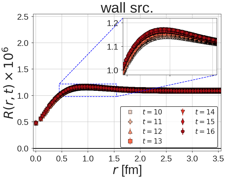
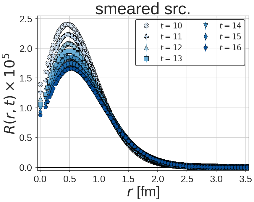
Figure 1: The $R$-correlator at $t=10-16$ from the wall source (Left) and the smeared source (Right).

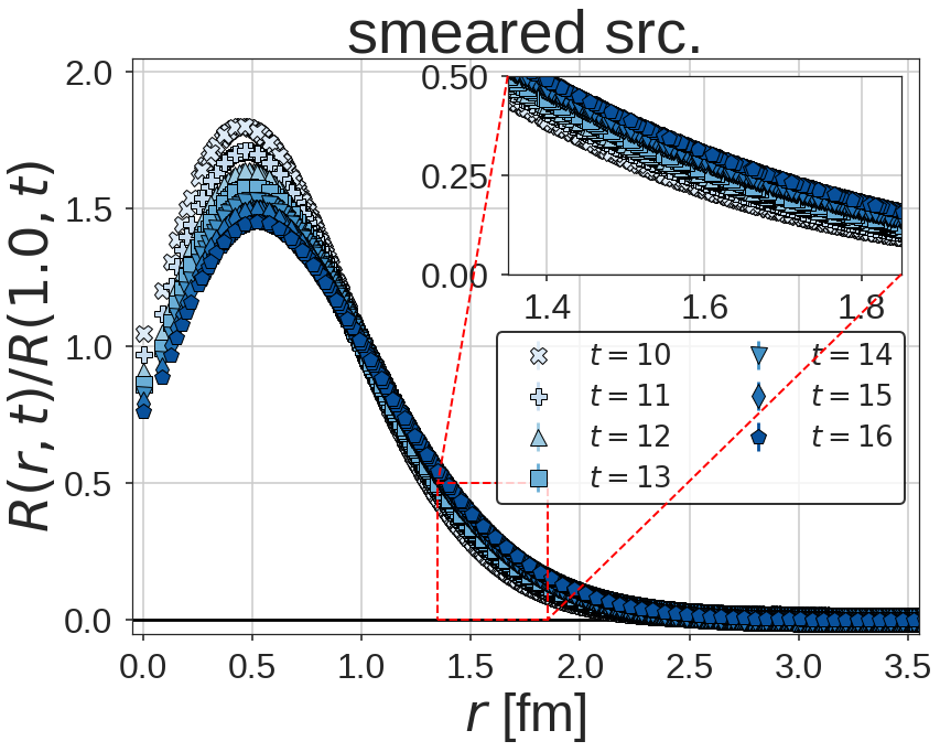
Figure 2: The normalized $R$-correlator at $t=10-16$ from the wall source (Left) and the smeared source (Right).

III.3 HAL QCD potential at the leading order

Let us now study the potential in the HAL QCD method at the leading order, $V_{0}^{\mathrm{LO}}(r)$. Fig. 3 shows the one for $\Xi\Xi$(¹S₀) and its breakups ($H_{0}$, $\partial/\partial t$ and $\partial^{2}/\partial t^{2}$ terms in Eq. (9)) on $L=64$ at $t=13$ from the wall source (Left) and the smeared source (Right). For the wall source, the $H_{0}$ term is dominant with sizable contributions from the $\partial/\partial t$ term, while the $\partial^{2}/\partial t^{2}$ term is negligible. The $\partial/\partial t$ term is not constant as a function of $r$, which indicates that there exist small but non-negligible contributions from the excited states in $R^{\mathrm{wall}}(\vec{r},t)$. For the smeared source, on the other hand, all terms are important. In particular, the $\partial/\partial t$ term (green triangles) shows substantial $r$-dependence indicating large contributions from the excited states in the smeared source. However, such dependence is cancelled by the $H_{0}$ term (blue squares) and is further corrected by the $\partial^{2}/\partial t^{2}$ term (black diamonds). The final results (red circles) with the smeared source and the wall source show qualitatively similar behaviors, i.e., the repulsive core at the short distance and the attractive pocket at the intermediate distance. This illustrates that the time-dependent HAL QCD method works well for extracting the $\Xi\Xi$ potential irrespective of the source structures.

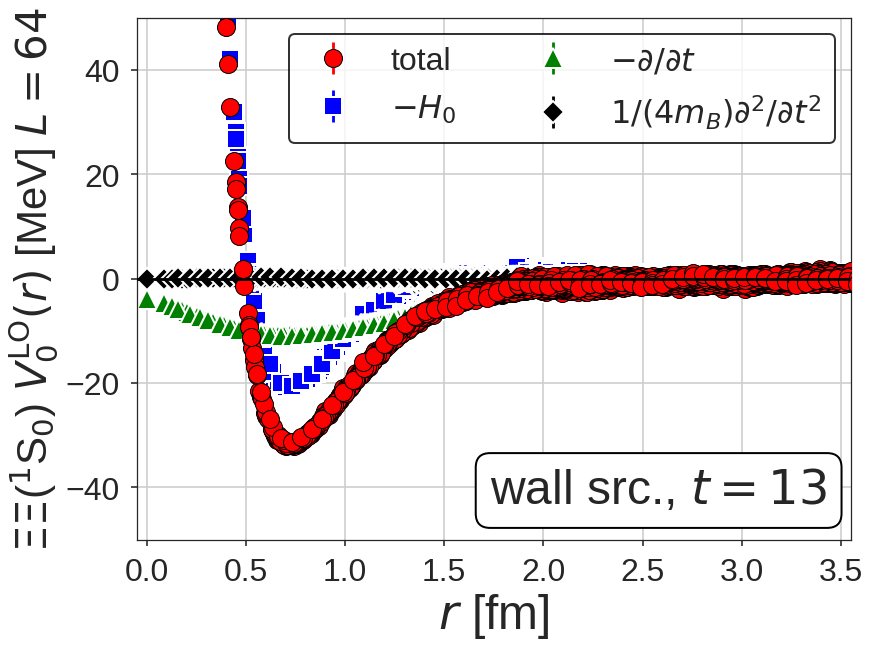
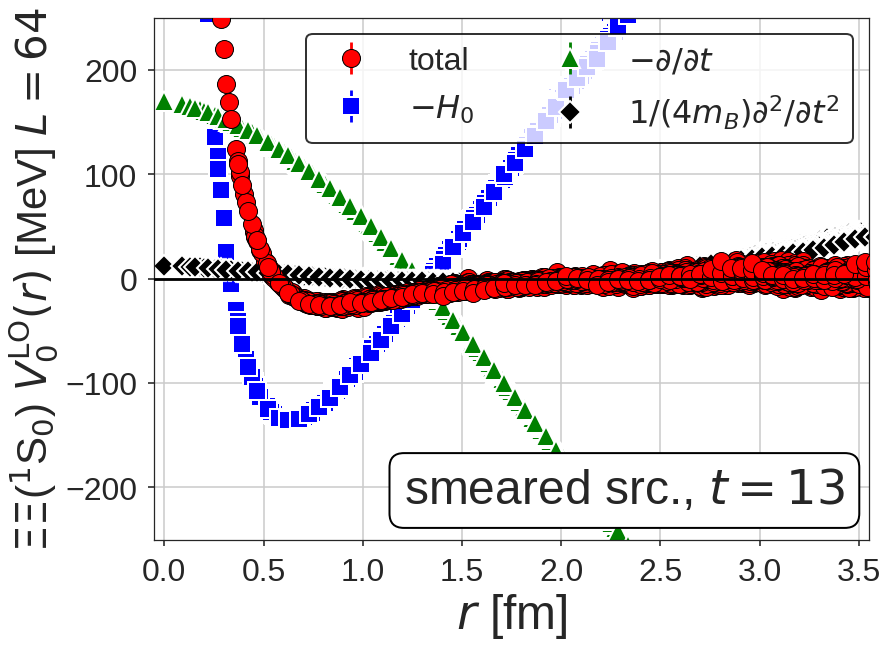
Figure 3: The potential at the leading order analysis, $V_{0}^{\mathrm{LO}}(r)$, (red circles) for the wall source (Left) and the smeared source (Right) at $t=13$. The blue squares, green triangles and black diamonds denote 1st, 2nd and 3rd terms in Eq. (9), respectively.

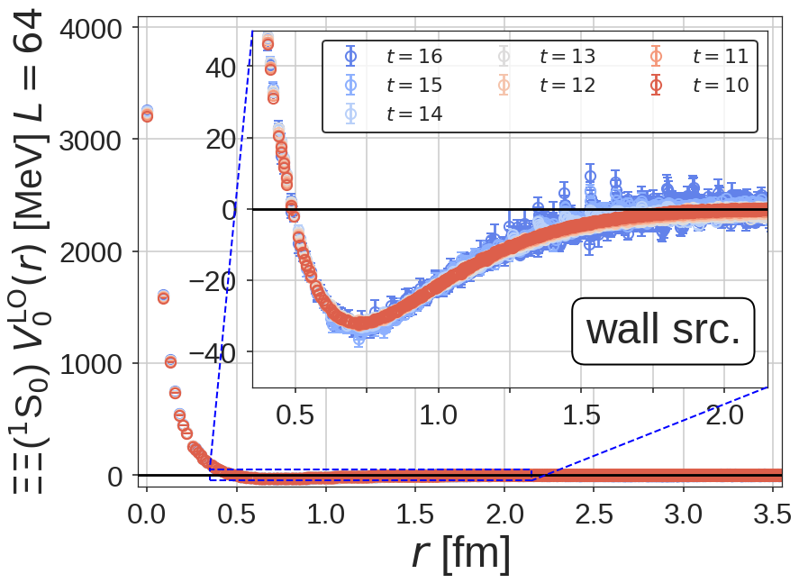
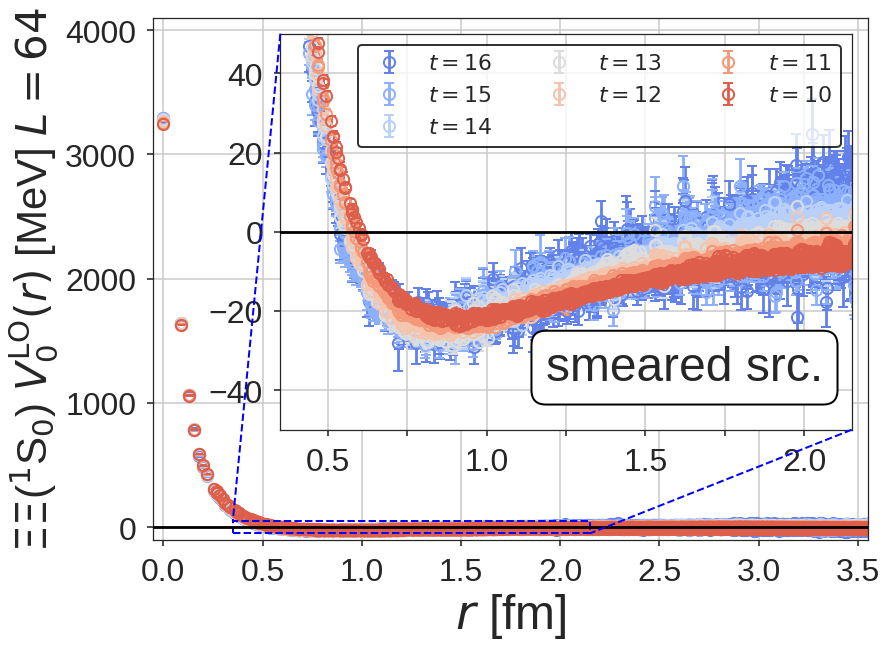
Figure 4: The potential at the leading order analysis, $V_{0}^{\mathrm{LO}}(r)$, for the wall source (Left) and the smeared source (Right) at $t=10-16$.

Shown in Fig. 4 is a comparison among the LO potentials ($V_{0}^{\mathrm{LO}}(r)$) for different $t$ in each source. For the wall source, the potentials at $t=10-16$ are consistent with each other within statistical errors, while those from the smeared source show the detectable $t$-dependence. Shown in Fig. 5 is a comparison of $V_{0}^{\mathrm{LO}}(r)$ between two sources at $t=10,12,14,16$. As $t$ increases, the LO potential from the smeared source gradually converges to that from the wall source. The relatively large $t$-dependence of the potentials from the smeared source as well as the remaining small discrepancy of potentials between two sources even at $t=16$ indicate that the N²LO analysis in the derivative expansion is necessary to understand the data from the smeared source. This is a natural consequence of the fact that the N²LO contributions in $V_{0}^{\mathrm{LO}}(r)$, $\nabla^{2}R(\vec{r},t)/R(\vec{r},t)$ ($\propto H_{0}$ term) in Eq. (11), is much more significant in the smeared source than the wall source as shown in Fig. 3.

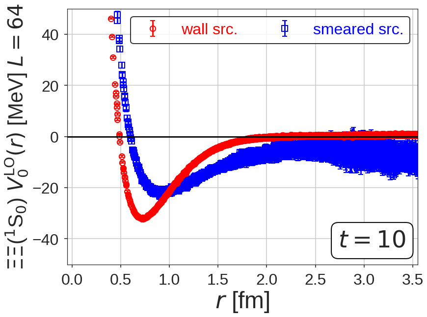
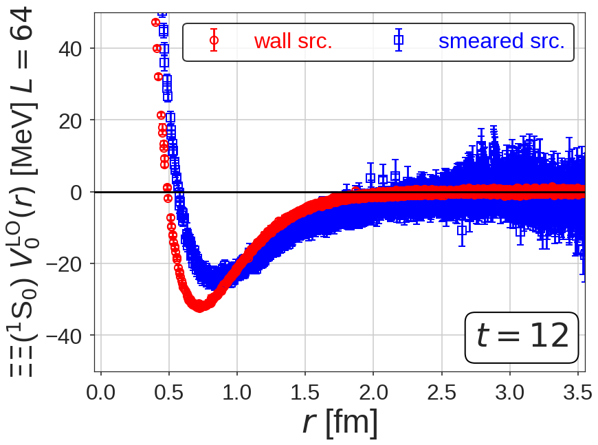
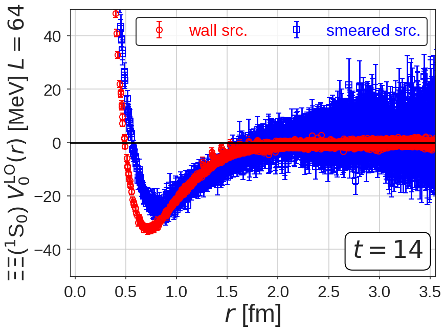
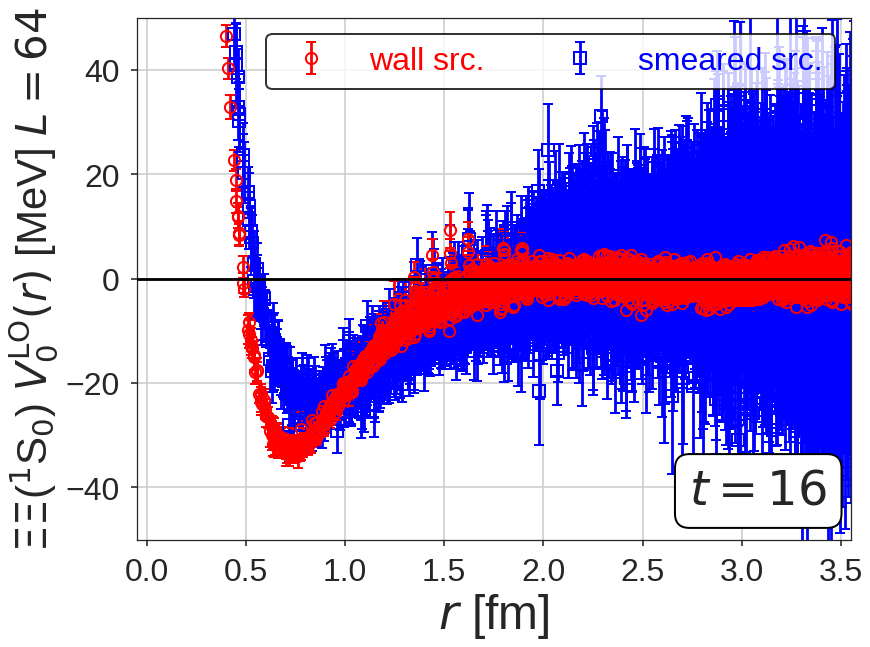
Figure 5: A comparison of the potential at the leading order analysis, $V_{0}^{\mathrm{LO}}(r)$, between the wall source (red circles) and the smeared source (blue squares) at $t=10,12,14,16$.

III.4 HAL QCD potential at the next-to-next-to-leading order

We next apply the N²LO analysis in the derivative expansion to $R$-correlators for both sources. The potential at the LO analysis, $V_{0}^{\mathrm{LO}}(r)$, and those at the N²LO analysis, $V_{0}^{\mathrm{N^{2}LO}}(r)$, $V_{2}^{\mathrm{N^{2}LO}}(r)$, satisfy the linear equations given by

$$\{V_{0}^{\mathrm{N^{2}LO}}(r)+V_{2}^{\mathrm{N^{2}LO}}(r)\nabla^{2}\}R^{\mathrm{source}}(\vec{r},t)=V_{0}^{\mathrm{LO(source)}}(r)R^{\mathrm{source}}(\vec{r},t),$$ (14)

where source = wall or smear.

To extract $V_{0,2}^{\mathrm{N^{2}LO}}(r)$, we first consider the following relation derived from Eq. (14),

$$D\times V_{2}^{\mathrm{N^{2}LO}}(r)=V_{0}^{\mathrm{LO(wall)}}(r)-V_{0}^{\mathrm{LO(smear)}}(r),$$ (15)

with $D\equiv\nabla^{2}R^{\mathrm{wall}}(\vec{r},t)/R^{\mathrm{wall}}(\vec{r},t)-\nabla^{2}R^{\mathrm{smear}}(\vec{r},t)/R^{\mathrm{smear}}(\vec{r},t)$. In order to avoid numerical instabilities caused by nearly zeros of $D$ when we divide the right hand side of Eq. (15), we extract $V_{2}^{\mathrm{N^{2}LO}}(r)$ directly from Eq. (15) with a fitting function, $V_{2}^{\mathrm{N^{2}LO}}(r)=b_{1}e^{-b_{2}(r-b_{{3}})^{2}}+b_{{4}}e^{-b_{{5}}(r-b_{{6}})^{2}}$ at each $t$. Once $V_{2}^{\mathrm{N^{2}LO}}(r)$ is obtained, $V_{0}^{\mathrm{N^{2}LO}}(r)$ can be determined from Eq. (11).

Fig. 6 shows the $V_{0}^{\mathrm{N^{2}LO}}(r)$ together with the $V_{0}^{\mathrm{LO(wall)}}(r)$ (Left), and the $V_{2}^{\mathrm{N^{2}LO}}(r)$ (Right) on $L=64$ at $t=13$. We multiply $V_{2}^{\mathrm{N^{2}LO}}(r)$ by $m_{\pi}^{2}$ to make its mass dimension $+1$ for a comparison to $V_{0}(r)$’s. We find that $V_{0}^{\mathrm{N^{2}LO}}(r)$ agrees well with the $V_{0}^{\mathrm{LO(wall)}}(r)$ except at short distances. We also find that $V_{2}^{\mathrm{N^{2}LO}}(r)$ is localized within the range of 1 fm, which is much shorter than the range of $V_{0}^{{\mathrm{LO(wall),N^{2}LO}}}(r)$. We note here that the negative sign of $V_{2}^{\mathrm{N^{2}LO}}(r)$ does not necessarily imply attraction, since the N²LO potential is given by $V_{2}^{\mathrm{N^{2}LO}}(r)\nabla^{2}$.

As already mentioned, $\nabla^{2}R(\vec{r},t)/R(\vec{r},t)$ from the smeared source is much larger than that of the wall source (see Fig. 3). Intuitively, this is because $R^{\mathrm{smear}}(r,t)$ ($R^{\mathrm{wall}}(r,t)$) contains larger (smaller) contributions from excited states and thus is more (less) sensitive to higher order terms in the derivative expansion of the potential. Therefore, the N²LO analysis is mandatory for the smeared source, while the LO analysis for the wall source leads to the potential which is almost identical to $V_{0}^{\mathrm{N^{2}LO}}(r)$.

Shown in Fig. 7 is the $t$-dependence of $V_{0,2}^{\mathrm{N^{2}LO}}(r)$ in the range of $t=13-16$. Since appreciable $t$-dependence is not seen within the error bars, the N⁴LO contribution is expected to be small.

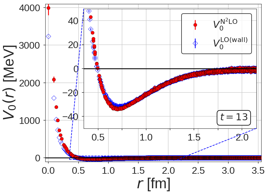
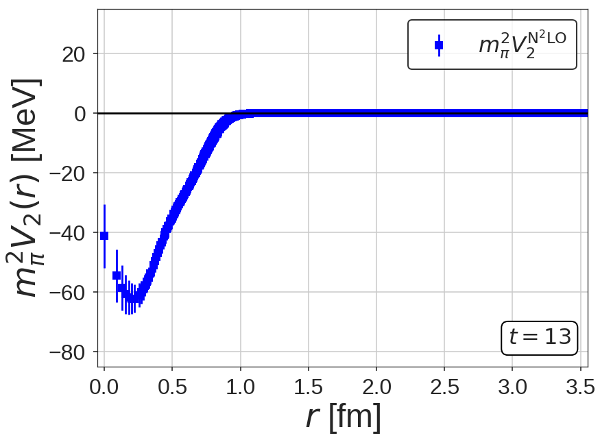
Figure 6: (Left) The LO potential at the N²LO analysis, $V_{0}^{\mathrm{N^{2}LO}}(r)$ (red circles), together with the potential at the LO analysis for the wall source, $V_{0}^{\mathrm{LO(wall)}}(r)$ (blue diamonds) at $t=13$. (Right) The N²LO potential at the N²LO analysis, $V_{2}^{\mathrm{N^{2}LO}}(r)$, multiplied by $m_{\pi}^{2}$.

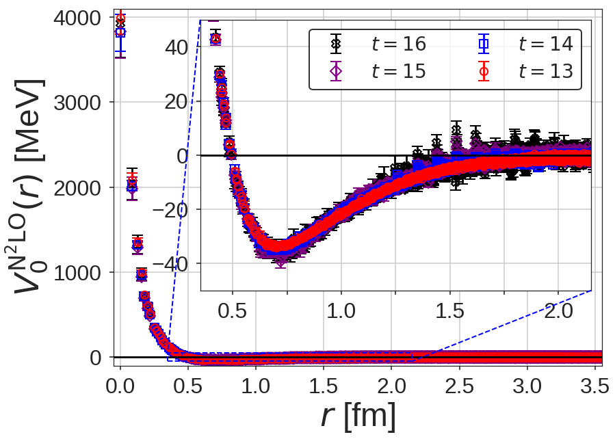
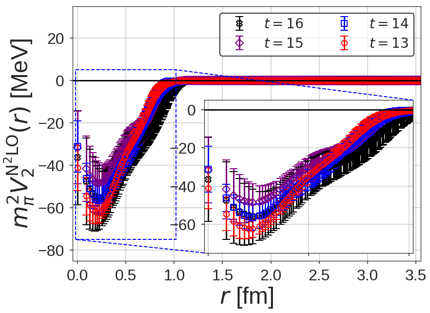
Figure 7: The LO (Left) and N²LO (Right) potentials at the N²LO analysis in the range of $t=13-16$.

III.5 Effect of the Inelastic states

Fig. 8 (Left) compares the effective mass of a single $\Xi$ for two sources. The smeared source is tuned to have a large overlap with the ground state of a single baryon, so that the corresponding effective mass shows a plateau at an earlier time than the case of the wall source. Eventually, the plateaux for the single $\Xi$ from two different sources converge at $t\gtrsim 16$. Shown in Fig. 8 (Right) is the $\Xi\Xi$ potential at the LO analysis for the wall source in the range of $t=9-17$. Unlike the case of the single $\Xi$, the resultant potential is stable for $t$ much less than $16$, suggesting that the systematic error originating from the inelastic contributions of the single-baryon cancels largely between the numerator and the denominator of the $R$-correlator for the wall source.

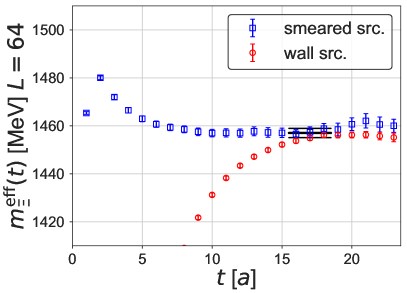
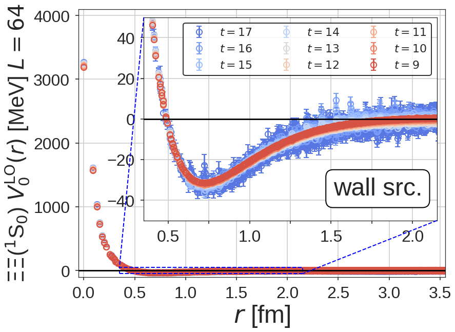
Figure 8: (Left) The effective mass of a single baryon $\Xi$ for the wall source (red circles) and the smeared source (blue squares). (Right) The potential at the LO analysis, $V_{0}^{\mathrm{LO}}(r)$, for the wall source at $t=9-17$.

III.6 Effect of the finite volume

In Fig. 9, we show the volume dependence of the potential at the LO analysis for the wall source at $t=13$ with $L=40$, $48$ and $64$. All the potentials are consistent with each other within statistical errors. This indicates that the artifact due to finite volume is negligible for the potential, mainly because the potential is short ranged.

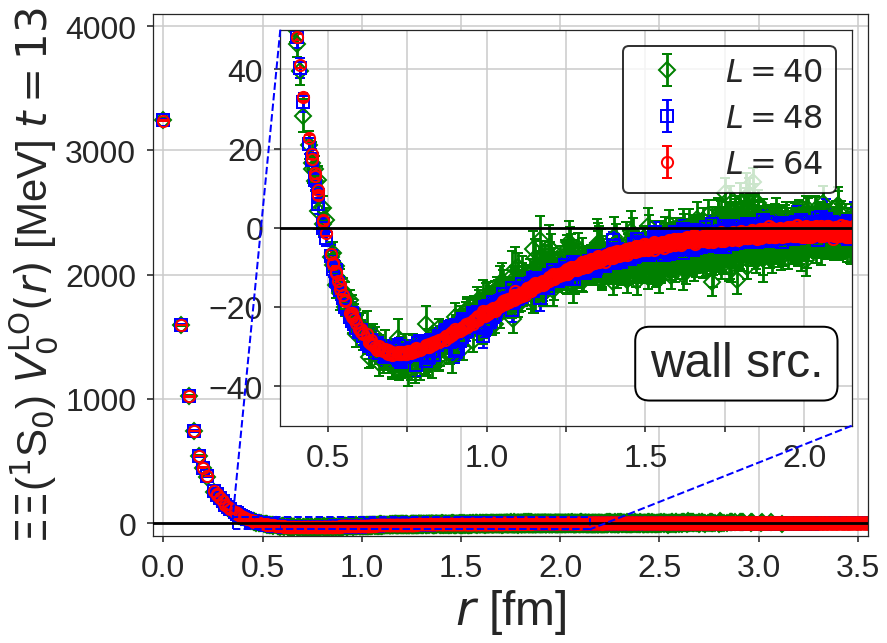
Figure 9: The potential at the LO analysis, $V_{0}^{\mathrm{LO}}(r)$, for the wall source on $L=40,48$ and $64$ at $t=13$.

IV Scattering phase shifts

In the previous section, we examine systematic uncertainties on the HAL QCD potential. In this section, we examine how these systematic uncertainties affect the physical observables such as the scattering phase shifts, in particular the effect of the derivative expansion. To calculate the scattering phase shifts, $\delta_{0}(k)$, we first fit the potentials by a sum of Gaussians, $V_{0}^{\mathrm{LO(wall),N^{2}LO}}(r)=\sum_{n=1,3,5,7}a_{n}e^{-a_{n+1}r^{2}}$ and $V_{2}^{\mathrm{N^{2}LO}}(r)=\sum_{n=1,4}b_{n}e^{-b_{n+1}(r-b_{n+2})^{2}}$. Resulting parameters are summarized in Table 2.

	$V_{0}^{\mathrm{LO(wall)}}(r)$	$V_{0}^{\mathrm{N^{2}LO}}(r)$		$V_{2}^{\mathrm{N^{2}LO}}(r)$
$a_{1}$	$0.8759\pm 0.0270$	$1.1426\pm 0.0621$	$b_{1}$	$-0.5291\pm 0.0418$
$a_{2}$	$1.2040\pm 0.0317$	$0.9332\pm 0.0871$	$b_{2}$	$0.0757\pm 0.0162$
$a_{3}$	$0.4261\pm 0.0128$	$0.4245\pm 0.0397$	$b_{3}$	$2.195\pm 0.333$
$a_{4}$	$0.3028\pm 0.0217$	$0.2358\pm 0.0382$	$b_{4}$	$-0.1091\pm 0.0194$
$a_{5}$	$0.2010\pm 0.0124$	$0.2415\pm 0.0410$	$b_{5}$	$0.2177\pm 0.0633$
$a_{6}$	$0.07373\pm 0.00364$	$0.07876\pm 0.00646$	$b_{6}$	$7.025\pm 0.464$
$a_{7}$	$-0.02922\pm 0.00148$	$-0.03005\pm 0.00159$
$a_{8}$	$0.008977\pm 0.000456$	$0.009107\pm 0.000467$

Table 2: Summary of fitting parameters for the LO and N²LO potentials in the lattice unit at $t=13$. The fitting range is $r\in[0,3.5]$ fm, and $\chi^{2}/\mathrm{dof}$ are 1.14, 1.01 and 0.0019 for $V_{0}^{\mathrm{LO(wall)}}(r)$, $V_{0}^{\mathrm{N^{2}LO}}(r)$ and $V_{2}^{\mathrm{N^{2}LO}}(r)$, respectively.

In Fig. 10, we show the comparison of the scattering phase shifts from $V_{0}^{\mathrm{LO(wall)}}(r)$, $V_{0}^{\mathrm{N^{2}LO}}(r)$ and $V_{0}^{\mathrm{N^{2}LO}}(r)+V_{2}^{\mathrm{N^{2}LO}}(r)\nabla^{2}$ at $t=13$. At low energies (Fig. 10 (Left)), the N²LO correction is found to be negligible, showing not only that the derivative expansion converges well but also that the LO analysis for the wall source is sufficiently good at low energies. The N²LO correction becomes non-negligible only at high energies as shown in Fig. 10 (Right) . We note that $(k/m_{\pi})^{2}=0.5$ corresponds to the energy from the threshold as $\Delta E\equiv W-2m_{B}\simeq 90$ MeV. The good convergence of the derivative expansion has been also observed for the $NN$ systems in the ¹S₀ and ³S₁ channels in quenched QCD with $m_{\pi}\simeq 530$ MeV Murano:2011nz and the $I=2$ $\pi\pi$ system in (2+1)-flavor QCD with $m_{\pi}\simeq 870$ MeV Kawai:2017goq .

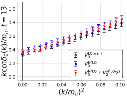
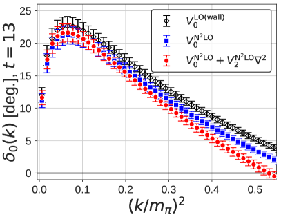
Figure 10: The scattering phase shifts in the form of $k\cot\delta_{0}(k)/m_{\pi}$ (Left) and $\delta_{0}(k)$ (Right) from $V_{0}^{\mathrm{LO(wall)}}(r)$ (black diamonds), $V_{0}^{\mathrm{N^{2}LO}}(r)$ (blue squares) and $V_{0}^{\mathrm{N^{2}LO}}(r)+V_{2}^{\mathrm{N^{2}LO}}(r)\nabla^{2}$ (red circles) at $t=13$.

The scattering length $a_{0}$ obtained through $\lim_{k\rightarrow 0}k\cot\delta_{0}(k)=1/a_{0}$ from $V_{0}^{\mathrm{LO(wall)}}(r)$, $V_{0}^{\mathrm{N^{2}LO}}(r)$ and $V_{0}^{\mathrm{N^{2}LO}}(r)+V_{2}^{\mathrm{N^{2}LO}}(r)\nabla^{2}$ at $t=13-16$ is shown in Fig. 11. The result indicates that the scattering length is almost insensitive to the degrees of the approximation but has a small variation in $t$, which is, however, within statistical errors. We thus conclude that the systematic errors from the derivative expansion and the inelastic state contaminations are well under control for this observable. Numerical values for the scattering length are summarized in Table 3, where the central value and statistical errors are evaluated at $t=13$ and the systematic errors are estimated from the $t$-dependence among $t=13-16$. We have checked that alternative fitting functions of the potential such as the combination of two Gaussians + (Yukawa)² form as employed in  Aoki:2012tk ; Yamada:2015cra give results consistent with those from the present fitting function within errors.

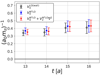
Figure 11: The scattering length $a_{0}$ in the form of $(a_{0}m_{\pi})^{-1}$ from $V_{0}^{\mathrm{LO(wall)}}(r)$ (black diamonds) , $V_{0}^{\mathrm{N^{2}LO}}(r)$ (blue squares) and $V_{0}^{\mathrm{N^{2}LO}}(r)+V_{2}^{\mathrm{N^{2}LO}}(r)\nabla^{2}$ (red circles) at $t=13-16$.

	$V_{0}^{\mathrm{LO(wall)}}(r)$	$V_{0}^{\mathrm{N^{2}LO}}(r)$	$V_{0}^{\mathrm{N^{2}LO}}(r)+V_{2}^{\mathrm{N^{2}LO}}(r)\nabla^{2}$
$(a_{0}m_{\pi})^{-1}$	0.341(36)(${}^{+70}_{-0}$)	0.368(39)(${}^{+65}_{-0}$)	0.352(36)(${}^{+80}_{-0}$)

Table 3: The scattering length $a_{0}$ in the form of $(a_{0}m_{\pi})^{-1}$ from $V_{0}^{\mathrm{LO(wall)}}(r)$, $V_{0}^{\mathrm{N^{2}LO}}(r)$ and $V_{0}^{\mathrm{N^{2}LO}}(r)+V_{2}^{\mathrm{N^{2}LO}}(r)\nabla^{2}$. The central values and statistical errors (in the first parenthesis) are evaluated at $t=13$, while the systematic errors (in the second) are estimated using the potentials at $t=14,15,16$.

V Finite volume formula and effective range expansion

Before closing the paper, we discuss the relation among the energy spectrum, the Lüscher’s finite volume formula and the effective range expansion (ERE). Once the energy shift of the two-body system on a finite volume is measured, the scattering phase shift is obtained by the Lüscher’s formula as

$$k\cot\delta_{0}(k)=\frac{1}{\pi L}\sum_{\vec{n}\in\mathbf{Z}^{3}}\frac{1}{|\vec{n}|^{2}-(kL/2\pi)^{2}},$$ (16)

where $k^{2}$ is related to the energy shift on a finite volume as $\Delta E_{L}=2\sqrt{m_{B}^{2}+k^{2}}-2m_{B}$. For the attractive interaction, $k^{2}$ can be negative on a finite volume. Note that the poles of the $S$-matrix with $k\cot\delta_{0}(k)=-\sqrt{-k^{2}}$ in the infinite volume correspond to the bound states. For the unbound two-body system, the asymptotic behavior of $\Delta E_{L}$ for large $L$ reads

$$\Delta E_{L}\simeq-\frac{2\pi a_{0}}{\mu L^{3}}\left[1+c_{1}\frac{a_{0}}{L}+c_{2}\left(\frac{a_{0}}{L}\right)^{2}\right]+\mathcal{O}(L^{-6}),$$ (17)

with the reduced mass $\mu$, the scattering length $a_{0}$, $c_{1}=-2.837297$, and $c_{2}=6.375183$ Luscher:1985dn ; Luscher:1990ux .

Let us now calculate $k^{2}$ from eigenvalue spectra of the Hamiltonian $H=H_{0}+V_{0}^{\mathrm{N^{2}LO}}(r)+V_{2}^{\mathrm{N^{2}LO}}(r)\nabla^{2}$ on the finite volume ($L=40,48,64$) for the $A_{1}^{+}$ representation of the cubic group, by employing fitted $V_{0}^{\mathrm{N^{2}LO}}(r)$ and $V_{2}^{\mathrm{N^{2}LO}}(r)$ at $L=64$ in Table 2. Fig. 12 (Left) shows the volume dependence of the lowest eigenvalues: The data are found to be well described by Eq. (17), which indicates that the system does not have a bound state. By fitting the data with Eq. (17), we obtain the scattering length as $(a_{0}m_{\pi})^{-1}=0.402(14)$ consistent with the values in Table 3, $(a_{0}m_{\pi})^{-1}=0.352(36){(^{+80}_{-0})}$.

As extensively discussed in Ref. Iritani:2017rlk , the ERE, $k\cot\delta_{0}(k)=1/a_{0}+(1/2)r_{\mathrm{eff}}k^{2}+\cdots$, provides a systematic and reliable way to relate the volume dependence of $\Delta E_{L}$, the scattering phase shifts and the bound state pole around $k^{2}=0$.

In Fig. 12 (Right), we plot the finite volume spectra on the $(k^{2},k\cot\delta_{0}(k))$ plane, using the lowest eigenvalues of $H$ on $L=40$, $48$, and $64$, and the eigenvalue of the first excited state on $L=64$. Note that the data (triangle, square and diamonds) and their errors are plotted together with the Lüscher’s formula (dotted lines). The blue band corresponds to the results obtained by solving the Schrödinger equation in the infinite volume. We find that the finite volume energy spectra at $k^{2}<0$ and $k^{2}>0$ are smoothly connected around $k^{2}=0$ along with the blue band, as is expected from the analytic properties of $S$-matrix and the ERE. In fact, the ERE at the NLO determined from these 4 data (pink band) is consistent with the blue band at $|(k/m_{\pi})^{2}|\lesssim 0.2$ within errors. One also observes that the positive intercept at $k^{2}=0$ ($1/a_{0}$) supports the conclusion from Fig. 12 (Left) that the system has no bound state.

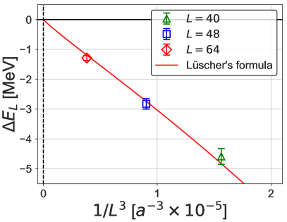
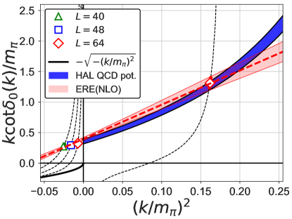
Figure 12: (Left) The lowest eigenenergies on finite volumes from the HAL QCD potential. The red line corresponds to the fit by the asymptotic Lüscher’s finite volume formula in the large $L$, Eq. (17). (Right) The scattering phase shifts from finite volume eigenenergies using Lüscher’s finite volume formula (green triangle, blue square, red diamonds), together with those in the infinite volume from the Schrödinger equation (blue band). The black dotted lines denote the constraints by the Lüscher’s finite volume formula, and the black solid line represents the bound state condition in the infinite volume. The red dashed line with the pink band corresponds to the NLO ERE analysis to the finite volume data.

VI Summary

In this paper, we have made critical investigations on the systematic uncertainties in the HAL QCD method. While the time-dependent HAL QCD method is free from the issue associated with the ground state saturation, the approximation of the energy-independent non-local potential by the derivative expansion introduces systematic uncertainties, so that it is necessary to check the errors introduced by the expansion.

We have performed the (2+1)-flavor lattice QCD calculation for the $\Xi\Xi(^{1}$S${}_{0})$ system at $m_{\pi}=0.51$ GeV. Using the four-point correlation functions from both wall and smeared quark sources, we have established the theoretical and numerical method to determine LO and N²LO potentials in the derivative expansion. Scattering phase shifts calculated from these potentials reveal that the LO potential is sufficient to reproduce observables at low energies ($k^{2}/m_{\pi}^{2}<0.1$), while the N²LO correction becomes non-negligible but remains small even at high energies ($k^{2}/m_{\pi}^{2}\simeq 0.5$), confirming the good convergence of the derivative expansion below the inelastic threshold for this particular system.

We have also found that the potential at the LO analysis for the wall source agrees with the LO potential at the N²LO analysis except at short distances and can reproduce the scattering phase shifts precisely at low energies. Other systematic uncertainties such as the inelastic state contaminations and the finite volume effect to the potential are investigated and are found to be well under control.

After establishing the reliability of the HAL QCD potential, we have calculated the eigenvalues of the Hamiltonian in finite boxes with the potential. The volume dependence of the lowest eigenvalues is well described by $1/L$-expansion for scattering states obtained from the Lüscher’s finite volume formula. We have also discussed the relation among the energy spectrum, phase shifts and the effective range expansion.

In a forthcoming paper Iritani:2018vfn , we will perform the spectral decomposition of the correlation function based on the eigenmodes of the Hamiltonian in a finite box with the HAL QCD potential, which will enable us to better understand the requirements for reliably extracting finite-volume energies.

Appendix A Non-locality vs. Energy dependence

Here we examine the relation between the energy-independent non-local potential with the derivative expansion, $U(\vec{r},\vec{r^{\prime}})=\{V_{0}(r)+V_{2}(r)\nabla^{2}+\cdots\}\delta(\vec{r}-\vec{r^{\prime}})$, and the energy-dependent local potential, $V^{\rm eff}(r;E)$. For simplicity, in this appendix, we restrict ourselves to the N²LO analysis. In other words, we assume as if the non-local potential were given exactly by $U(\vec{r},\vec{r^{\prime}})=\{V_{0}(r)+V_{2}(r)\nabla^{2}\}\delta(\vec{r}-\vec{r^{\prime}})$.

In this case, it is easy to show that the Schrödinger equation with this non-local potential, given by

$$\left[-\frac{\nabla^{2}}{2\mu}+V_{0}(r)+V_{2}(r)\nabla^{2}\right]\psi(\vec{r})=E\psi(\vec{r}),\qquad\mu=m_{B}/2,$$ (18)

can be written in terms of the energy-dependent local potential as

$$\left[-\frac{\nabla^{2}}{2\mu}+V^{\rm eff}(r;E)\right]\psi(\vec{r})=E\psi(\vec{r}),$$ (19)

where

$$V^{\mathrm{eff}}(r;E)\equiv\frac{V_{0}(r)-m_{B}EV_{2}(r)}{1-m_{B}V_{2}(r)},$$ (20)

which gives an exact relation between the energy-independent non-local potential and the energy-dependent local potential (within the N²LO analysis). Although both descriptions for the potential are theoretically equivalent as shown above, we stress that the HAL QCD method is based on the energy-independent non-local potential, which can be extracted from arbitrary linear combinations of the NBS wave function $\psi^{W}(\vec{r})$ thanks to the time dependent method, while the energy-dependent local potential requires the eigenstate saturation, which is difficult to achieve in practice, particularly for excited states. Also $V^{\mathrm{eff}}(r;E)$ gives the correct scattering phase shift at each $E$ (one potential per energy), while $V_{0}(r)+V_{2}(r)\nabla^{2}$ gives the correct scattering phase shifts (within the N²LO analysis) at all $E\leq E_{\rm th}$ (one potential for all).

Fig. 13 shows the energy dependence of $V^{\mathrm{eff}}(r;E)$ from $E=10$ MeV to $E=200$ MeV. In these figures, we use $V_{0}^{\mathrm{N^{2}LO}}(r)$ and $V_{2}^{\mathrm{N^{2}LO}}(r)$ obtained at $t=13$ for $V_{0}(r)$ and $V_{2}(r)$, respectively. The energy dependent correction is small at low energies, while it is no longer negligible at higher energies. As the energy increases, the attractive pocket at an intermediate distance becomes shallower and the radius of the repulsive core becomes larger.

This result also demonstrates how the non-locality of the energy-independent potential, $U(r,r^{\prime})$, (Note that $V_{0}(r)$, $V_{2}(r),\cdots$ are energy-independent by definition ), is related to the energy dependence of the local potential, $V^{\mathrm{eff}}(r;E)$.

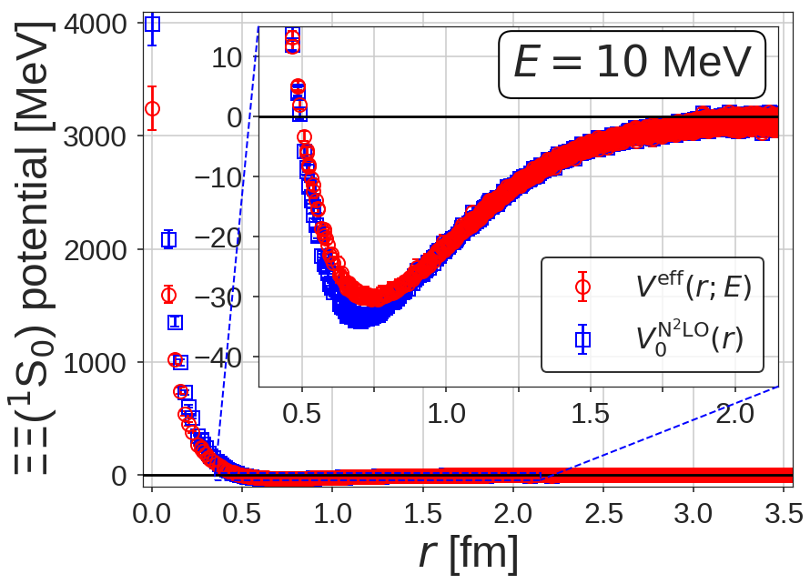
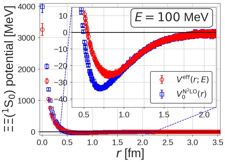
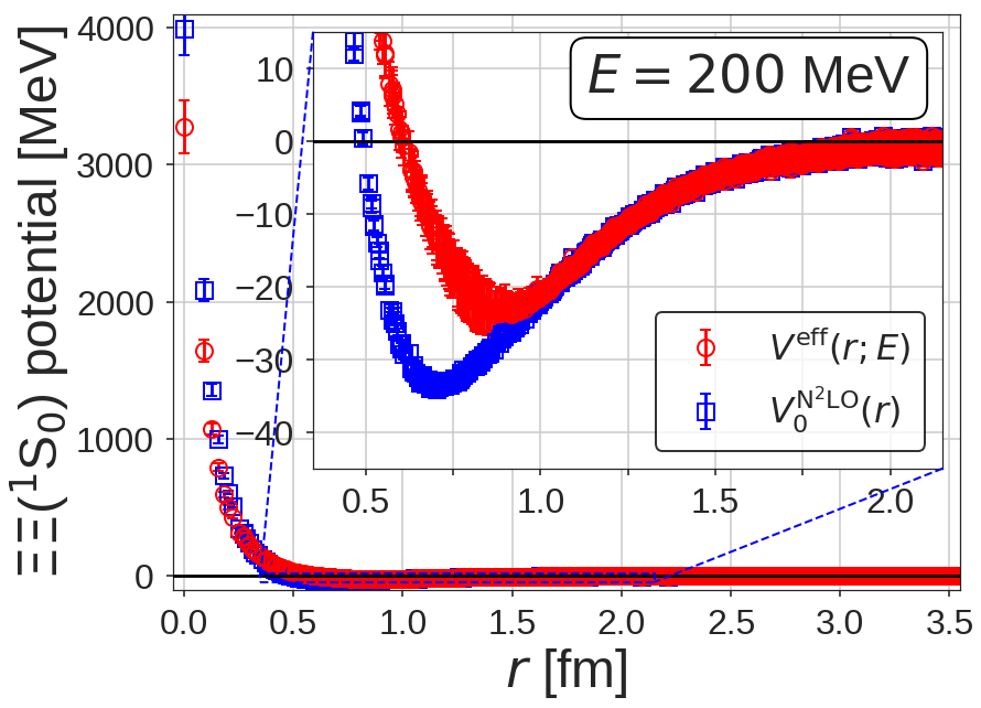
Figure 13: The energy dependence of the effective potential, $V^{\mathrm{eff}}(r;E)$, (red circles) compared with the LO potential at the N²LO analysis, $V_{0}^{\mathrm{N^{2}LO}}(r)$ (blue squares) at $E=10$ MeV (Top Left), $E=50$ MeV (Top Right), $E=100$ MeV (Bottom Left) and $E=200$ MeV (Bottom Right).

References

- (1) T. Yamazaki, K. i. Ishikawa, Y. Kuramashi and A. Ukawa, Phys. Rev. D 92, 014501 (2015) [arXiv:1502.04182 [hep-lat]], and references therein.
- (2) M. L. Wagman, F. Winter, E. Chang, Z. Davoudi, W. Detmold, K. Orginos, M. J. Savage and P. E. Shanahan, Phys. Rev. D 96, 114510 (2017) [arXiv:1706.06550 [hep-lat]], and references therein.
- (3) E. Berkowitz, T. Kurth, A. Nicholson, B. Joo, E. Rinaldi, M. Strother, P. M. Vranas and A. Walker-Loud, Phys. Lett. B 765, 285 (2017) [arXiv:1508.00886 [hep-lat]], and references therein.
- (4) M. Lüscher, Commun. Math. Phys. 104, 177 (1986); ibid., 105, 153 (1986).
- (5) M. Lüscher, Nucl. Phys. B 354, 531 (1991)
- (6) N. Ishii, S. Aoki and T. Hatsuda, Phys. Rev. Lett. 99, 022001 (2007) [arXiv:nucl-th/0611096].
- (7) S. Aoki, T. Hatsuda and N. Ishii, Prog. Theor. Phys. 123, 89 (2010) [arXiv:0909.5585 [hep-lat]].
- (8) N. Ishii et al. [HAL QCD Collaboration], Phys. Lett. B712, 437 (2012)
- (9) S. Aoki et al. [HAL QCD Collaboration], PTEP 2012, 01A105 (2012) [arXiv:1206.5088 [hep-lat]].
- (10) S. Aoki, B. Charron, T. Doi, T. Hatsuda, T. Inoue and N. Ishii, Phys. Rev. D 87, 034512 (2013) [arXiv:1212.4896 [hep-lat]].
- (11) T. Iritani et al. [HAL QCD Collaboration], JHEP 1610, 101 (2016) [arXiv:1607.06371 [hep-lat]].
- (12) T. Iritani et al., Phys. Rev. D 96, 034521 (2017) [arXiv:1703.07210 [hep-lat]].
- (13) S. Aoki, T. Doi and T. Iritani, EPJ Web Conf. 175, 05006 (2018) [arXiv:1707.08800 [hep-lat]].
- (14) T. Iritani et al., arXiv:1812.08539 [hep-lat].
- (15) R. Haag, Phys. Rev. 112, 669 (1958)
- (16) T. Yamazaki, K. i. Ishikawa, Y. Kuramashi and A. Ukawa, Phys. Rev. D 86, 074514 (2012) [arXiv:1207.4277 [hep-lat]].
- (17) D. Kawai et al. [HAL QCD Collaboration], Prog. Theor. Exp. Phys. 2018, 043B04 (2018) [arXiv:1711.01883 [hep-lat]].
- (18) T. Doi and M. G. Endres, Comput. Phys. Commun. 184, 117 (2013) [arXiv:1205.0585 [hep-lat]].
- (19) R. A. Briceno, J. J. Dudek and R. D. Young, Rev. Mod. Phys. 90, no. 2, 025001 (2018) [arXiv:1706.06223 [hep-lat]], and references therein.
- (20) M. Luscher and U. Wolff, Nucl. Phys. B 339, 222 (1990).
- (21) K. Murano, N. Ishii, S. Aoki and T. Hatsuda, Prog. Theor. Phys. 125, 1225 (2011) [arXiv:1103.0619 [hep-lat]].
- (22) M. Yamada et al. [HAL QCD Collaboration], PTEP 2015 , 071B01 (2015) [arXiv:1503.03189 [hep-lat]].
- (23) T. Amagasa et al., J. Phys. Conf. Ser. 664, 042058 (2015)
- (24) http://www.lqcd.org/ildg, http://www.jldg.org
- (25) Columbia Physics System (CPS), http://usqcd-software.github.io/CPS.html
- (26) Bridge++, http://bridge.kek.jp/Lattice-code/
- (27) M. Schröck and H. Vogt, Comput. Phys. Commun. 184, 1907 (2013) [arXiv:1212.5221 [hep-lat]].
- (28) T. Boku et al., PoS LATTICE 2012, 188 (2012) [arXiv:1210.7398 [hep-lat]].
- (29) M. Terai et al., IPSJ Transactions on Advanced Computing Systems, Vol.6 No.3, 43-57 (Sep. 2013) (in Japanese).
- (30) S. Aoki, T. Doi, T. Hatsuda and N. Ishii, Phys. Rev. D 98, 038501 (2018) [arXiv:1711.09344 [hep-lat]].