Planning and Learning with Stochastic Action Sets

Craig Boutilier, Alon Cohen, Amit Daniely, Avinatan Hassidim,
Yishay Mansour, Ofer Meshi, Martin Mladenov, Dale Schuurmans
Google Research, Mountain View, CA, USA
{cboutilier,aloncohen,amitdaniely,avinatan,mansour,meshi,schuurmans}@google.com
Abstract

In many practical uses of reinforcement learning (RL) the set of actions available at a given state is a random variable, with realizations governed by an exogenous stochastic process. Somewhat surprisingly, the foundations for such sequential decision processes have been unaddressed. In this work, we formalize and investigate MDPs with stochastic action sets (SAS-MDPs) to provide these foundations. We show that optimal policies and value functions in this model have a structure that admits a compact representation. From an RL perspective, we show that Q-learning with sampled action sets is sound. In model-based settings, we consider two important special cases: when individual actions are available with independent probabilities; and a sampling-based model for unknown distributions. We develop poly-time value and policy iteration methods for both cases; and in the first, we offer a poly-time linear programming solution.

1 Introduction

Markov decision processes (MDPs) are the standard model for sequential decision making under uncertainty, and provide the foundations for reinforcement learning (RL). With the recent emergence of RL as a practical AI technology in combination with deep learning [14, 15], new use cases are arising that challenge basic MDP modeling assumptions. One such challenge is that many practical MDP and RL problems have stochastic sets of feasible actions; that is, the set $A_{s}$ of feasible actions at state $s$ varies stochastically with each visit to $s$. For instance, in online advertising, the set of available ads differs at distinct occurrences of the same state (e.g., same query, user, contextual features), due to exogenous factors like campaign expiration or budget throttling. In recommender systems with large item spaces, often a set of candidate recommendations is first generated, from which top scoring items are chosen; exogenous factors often induce non-trivial changes in the candidate set. With the recent application of MDP and RL models in ad serving and recommendation [6, 11, 4, 3, 2, 19, 20, 13], understanding how to capture the stochastic nature of available action sets is critical.

Somewhat surprisingly, this problem seems to have been largely unaddressed in the literature. Standard MDP formulations [18] allow each state $s$ to have its own feasible action set $A_{s}$, and it is not uncommon to allow the set $A_{s}$ to be non-stationary or time-dependent. However, they do not support the treatment of $A_{s}$ as a stochastic random variable. In this work, we: (a) introduce the stochastic action set MDP (SAS-MDP) and provide its theoretical foundations; (b) describe how to account for stochastic action sets in model-free RL (e.g., Q-learning); and (c) develop tractable algorithms for solving SAS-MDPs in important special cases.

An obvious way to treat this problem is to embed the set of available actions into the state itself. This provides a useful analytical tool, but it does not immediately provide tractable algorithms for learning and optimization, since each state is augmented with all possible subsets of actions, incurring an exponential blow up in state space size. To address this issue, we show that SAS-MDPs possess an important property: the Q-value of an available action $a$ is independent of the availability of other actions. This allows us to prove that optimal policies can be represented compactly using (state-specific) decision lists (or orderings) over the action set.

This special structure allows one to solve the SAS RL problem effectively using, for example, Q-learning. We also devise model-based algorithms that exploit this policy structure. We develop value and policy iteration schemes, showing they converge in a polynomial number of iterations (w.r.t.Β the size of the underlying β€œbase” MDP). We also show that per-iteration complexity is polynomial time for two important special forms of action availability distribution: (a) when action availabilities are independent, both methods are exact; (b) when the distribution over sets $A_{s}$ is sampleable, we obtain approximation algorithms with polynomial sample complexity. In fact, policy iteration is strongly polynomial under additional assumptions (for a fixed discount factor). We show that a linear program for SAS-MDPs can be solved in polynomial time as well. Finally, we offer a simple empirical demonstration of the importance of accounting for stochastic action availability when computing an MDP policy.

Additional discussion and full proofs of all results can be found in a longer version of this paper [5].

2 MDPs with Stochastic Action Sets

We first introduce SAS-MDPs and provide a simple example illustrating how action availability impacts optimal decisions. See [18] for more background on MDPs.

2.1 The SAS-MDP Model

Our formulation of MDPs with Stochastic Action Sets (SAS-MDPs) derives from a standard, finite-state, finite-action MDP (the base MDP) $\mathcal{M}$, with $n$ states $S$, base actions $B_{s}$ for $s\in S$, and transition and reward functions, $P:S\times B\rightarrow\Delta(S)$ and $r:S\times B\rightarrow\mathbb{R}$. We use ps,sβ€²ksubscriptsuperscriptπ‘π‘˜π‘ superscript𝑠′p^{k}_{s,s^{\prime}} and rsksubscriptsuperscriptπ‘Ÿπ‘˜π‘ r^{k}_{s} to denote the probability of transition to $s^{\prime}$ and the accrued reward, respectively, when action $k$ is taken at state $s$. For notational ease, we assume that feasible action sets for each $s\in S$ are identical, so $B_{s}=B$ (allowing distinct base sets at different states has no impact on what follows). Let $|B|=m$ and $M=|S\times B|=nm$. We assume an infinite-horizon, discounted objective with fixed discount rate $\gamma$, $0\leq\gamma<1$.

In a SAS-MDP, the set of actions available at state $s$ at any stage $t$ is a random subset $A^{(t)}_{s}\subseteq B$. We assume a family of action availability distributions $P_{s}\in\Delta(2^{B})$ defined over the powerset of $B$. These can depend on $s\in S$ but are otherwise history-independent, hence $\Pr(A^{(t)}_{s}|s^{(1)},\ldots,s^{(t)})=\Pr(A^{(t)}_{s}|s^{(t)})$. Only actions $k\in A^{(t)}_{s}$ in the realized available action set can be executed at stage $t$. Apart from this, the dynamics of the MDP is unchanged: when an (available) action is taken, state transitions and rewards are prescribed as in the base MDP. In what follows, we assume that some action is always available, i.e., $\Pr(A^{(t)}_{s}=\emptyset)=0$ for all $s,t$.111Models that trigger process termination when $A^{(t)}_{s}=\emptyset$ are well-defined, but we set aside this model variant here. Note that a SAS-MDP does not conform to the usual definition of an MDP.

2.2 Example

The following simple MDP shows the importance of accounting for stochastic action availability when making decisions. The MDP below has two states. Assume the agent starts at state $s_{1}$, where two actions (indicated by directed edges for their transitions) are always available: one ($\mathit{Stay}$) stays at $s_{1}$, and the other ($\mathit{Go}$) transitions to state $s_{2}$, both with reward $1/2$. At $s_{2}$, the action $\mathit{Down}$ returns to $s_{1}$, is always available and has reward 0. A second action $\mathit{Up}$ also returns to $s_{1}$, but is available with only probability $p$ and has reward 1. [Uncaptioned image]

A naive solution that ignores action availability is as follows: we first compute the optimal $Q$-function assuming all actions are available (this can be derived from the optimal value function, computed using standard techniques). Then at each stage, we use the best action available at the current state where actions are ranked by Q-value. Unfortunately, this leads to a suboptimal policy when the $\mathit{Up}$ action has low availability, specifically if $p<0.5$.

The best naive policy always chooses to move to $s_{2}$ from $s_{1}$; at $s_{2}$, it picks the best action available. This yields a reward of $1/2$ at even stages, and an expected reward of $p$ at odd stages. However, by anticipating the possibility that action $\mathit{Up}$ is unavailable at $s_{2}$, the optimal (SAS) policy always stays at $s_{1}$, obtaining reward $1/2$ at all stages. For $p<1/2$, the latter policy dominates the former: the plot on the right shows the fraction of the optimal (SAS) value lost by the naive policy ($Std$) as a function of the availability probability $p$. This example also illustrates that as action availability probabilities approach $1$, the optimal policy for the base MDP is also optimal for the SAS-MDP.

2.3 Related Work

While a general formulation of MDPs with stochastic action availability does not appear in the literature, there are two strands of closely related work. In the bandits literature, sleeping bandits are defined as bandit problems in which the arms available at each stage are determined randomly or adversarially (sleeping experts are similar, with complete feedback being provided rather than bandit feedback) [10, 9]. Best action orderings (analogous to our decision list policies for SAS-MDPs) are often used to define regret in these models. The goal is to develop exploration policies to minimize regret. Since these models have no state, if the action reward distributions are known, the optimal policy is trivial: always take the best available action. By contrast, a SAS-MDP, even a known model, induces a difficult optimization problem, since the quality of an action depends not just on its immediate reward, but also on the availability of actions at reachable (future) states. This is our focus.

The second closely related branch of research comes from the field of stochastic routing. The β€œCanadian Traveller Problem”—the problem of minimizing travel time in a graph with unavailable edgesβ€”was introduced by Papadimitriou and YannakakisΒ [1], who gave intractability results (under much weaker assumptions about edge availability, e.g. adversarial). Poliyhondrous and TsitsiklisΒ [17] consider a stochastic version of the problem, where edge availabilities are random but static (and any edge observed to be unavailable remains so throughout the scenario). Most similar to our setting is the work of Nikolova and KargerΒ [16], who discuss the case of resampling edge costs at each node visit; however, the proposed solution is well-defined only when the edge costs are finite and does not easily extend to unavailable actions/infinite edge costs. Due to the specificity of their modeling assumptions, none of the solutions found in this line of research can be adapted in a straightforward way to SAS-MDPs.

3 Two Reformulations of SAS-MDPs

The randomness of feasible actions means that SAS-MDPs do not conform to the usual definition of an MDP. In this section, we develop two reformulations of SAS-MDPs that transform them into MDPs. We discuss the relative advantages of each, outline key properties and relationships between these models, and describe important special cases of the SAS-MDP model itself.

3.1 The Embedded MDP

We first consider a reformulation of the SAS-MDP in which we embed the (realized) available action set into the state space itself. This is a straightforward way to recover a standard MDP. The embedded MDP $\mathcal{M}_{e}$ for a SAS-MDP has state space $S_{e}=\{s\circ A:s\in S,A\subseteq B\}$, with $s\circ A$ having feasible action set $A$.222Embedded states whose embedded action subsets have zero probability are unreachable and can be ignored. The history independence of $P_{s}$ allows transitions to be defined as:

ps∘A,sβ€²βˆ˜Aβ€²k=P​(sβ€²βˆ˜Aβ€²|s∘A,k)=ps,sβ€²k​Ps′​(Aβ€²),βˆ€k∈A.formulae-sequencesubscriptsuperscriptπ‘π‘˜π‘ π΄superscript𝑠′superscript𝐴′𝑃conditionalsuperscript𝑠′superscriptπ΄β€²π‘ π΄π‘˜subscriptsuperscriptπ‘π‘˜π‘ superscript𝑠′subscript𝑃superscript𝑠′superscript𝐴′for-allπ‘˜π΄p^{k}_{s\circ A,s^{\prime}\circ A^{\prime}}=P(s^{\prime}\circ A^{\prime}|s\circ A,k)=p^{k}_{s,s^{\prime}}P_{s^{\prime}}(A^{\prime}),\;\;\forall k\in A.

Rewards are defined similarly: rk​(s∘A)=rk​(s)superscriptπ‘Ÿπ‘˜π‘ π΄superscriptπ‘Ÿπ‘˜π‘ r^{k}(s\circ A)=r^{k}(s) for $k\in A$.

In our earlier example, the embedded MDP has three states: $s_{1}\circ\{\mathit{Stay},\mathit{Go}\},s_{2}\circ\{\mathit{Up},\mathit{Down}\},s_{2}\circ\{\mathit{Down}\}$ (other action subsets have probability 00 hence their corresponding embedded states are unreachable). The feasible actions at each state are given by the embedded action set, and the only stochastic transition occurs when $\mathit{Go}$ is taken at $s_{1}$: it moves to $s_{2}\circ\{\mathit{Up},\mathit{Down}\}$ with probability $p$ and $s_{2}\circ\{\mathit{Down}\}$ with probability $1-p$.

Clearly, the induced reward process and dynamics are Markovian, hence $\mathcal{M}_{e}$ is in fact an MDP under the usual definition. Given the natural translation afforded by the embedded MDP, we view this as providing the basic β€œsemantic” underpinnings of the SAS-MDP model. This translation affords the use of standard MDP analytical tools and methods.

A (stationary, determinstic, Markovian) policy $\pi:S_{e}\rightarrow B$ for $\mathcal{M}_{e}$ is restricted so that π​(s∘A)∈Aπœ‹π‘ π΄π΄\pi(s\circ A)\in A. The policy backup operator $T^{\pi}_{e}$ and Bellman operator $T^{\ast}_{e}$ for $\mathcal{M}_{e}$ decompose naturally as follows:

Teπ​Ve​(s∘As)=rsπ​(s∘As)+subscriptsuperscriptπ‘‡πœ‹π‘’subscript𝑉𝑒𝑠subscript𝐴𝑠limit-fromsubscriptsuperscriptπ‘Ÿπœ‹π‘ subscript𝐴𝑠𝑠\displaystyle T^{\pi}_{e}V_{e}(s\circ A_{s})=r^{\pi(s\circ A_{s})}_{s}+
Ξ³β€‹βˆ‘sβ€²ps,s′π​(s∘As)β€‹βˆ‘Asβ€²βŠ†BPs′​(Asβ€²)​Ve​(sβ€²βˆ˜Asβ€²),𝛾subscriptsuperscript𝑠′subscriptsuperscriptπ‘πœ‹π‘ subscript𝐴𝑠𝑠superscript𝑠′subscriptsubscript𝐴superscript𝑠′𝐡subscript𝑃superscript𝑠′subscript𝐴superscript𝑠′subscript𝑉𝑒superscript𝑠′subscript𝐴superscript𝑠′\displaystyle\qquad\gamma\sum_{s^{\prime}}p^{\pi(s\circ A_{s})}_{s,s^{\prime}}\sum_{A_{s^{\prime}}\subseteq B}P_{s^{\prime}}(A_{s^{\prime}})V_{e}(s^{\prime}\circ A_{s^{\prime}}), (1)
Teβˆ—β€‹Ve​(s∘As)=maxk∈As⁑rsk+subscriptsuperscriptπ‘‡βˆ—π‘’subscript𝑉𝑒𝑠subscript𝐴𝑠limit-fromsubscriptπ‘˜subscript𝐴𝑠subscriptsuperscriptπ‘Ÿπ‘˜π‘ \displaystyle T^{\ast}_{e}V_{e}(s\circ A_{s})=\max_{k\in A_{s}}r^{k}_{s}+
Ξ³β€‹βˆ‘sβ€²ps,sβ€²kβ€‹βˆ‘Asβ€²βŠ†BPs′​(Asβ€²)​Ve​(sβ€²βˆ˜Asβ€²)𝛾subscriptsuperscript𝑠′subscriptsuperscriptπ‘π‘˜π‘ superscript𝑠′subscriptsubscript𝐴superscript𝑠′𝐡subscript𝑃superscript𝑠′subscript𝐴superscript𝑠′subscript𝑉𝑒superscript𝑠′subscript𝐴superscript𝑠′\displaystyle\qquad\gamma\sum_{s^{\prime}}p^{k}_{s,s^{\prime}}\sum_{A_{s^{\prime}}\subseteq B}P_{s^{\prime}}(A_{s^{\prime}})V_{e}(s^{\prime}\circ A_{s^{\prime}}) (2)

Their fixed points, $V^{\pi}_{e}$ and $V^{\ast}_{e}$ respectively, can be expressed similarly.

Obtaining an MDP from an SAS-MDP via action-set embedding comes at the expense of a (generally) exponential blow-up in the size of the state space, which can increase by a factor of $2^{|B|}$.

3.2 The Compressed MDP

The embedded MDP provides a natural semantics for SAS-MDPs, but is problematic from an algorithmic and learning perspective given the state space blow-up. Fortunately, the history independence of the availability distributions gives rise to an effective, compressed representation. The compressed MDP $\mathcal{M}_{c}$ recasts the embedded MDP in terms of the original state space, using expectations to express value functions, policies, and backups over $S$ rather than over the (exponentially larger) $S_{e}$. As we will see below, the compressed MDP induces a blow-up in action space rather than state space, but offers significant computational benefits.

Formally, the state space for $\mathcal{M}_{c}$ is $S$. To capture action availability, the feasible action set for $s\in S$ is the set of state policies, or mappings ΞΌs:2Bβ†’B:subscriptπœ‡π‘ β†’superscript2𝐡𝐡\mu_{s}:2^{B}\rightarrow B satisfying ΞΌs​(As)∈Assubscriptπœ‡π‘ subscript𝐴𝑠subscript𝐴𝑠\mu_{s}(A_{s})\in A_{s}. In other words, once we reach $s$, ΞΌssubscriptπœ‡π‘ \mu_{s} dictates what action to take for any realized action set $A_{s}$. A policy for $\mathcal{M}_{c}$ is a family ΞΌc={ΞΌs:s∈S}subscriptπœ‡π‘conditional-setsubscriptπœ‡π‘ π‘ π‘†\mu_{c}=\{\mu_{s}:s\in S\} of such state policies. Transitions and rewards use expectations over $A_{s}$:

ps,sβ€²ΞΌs=βˆ‘AsβŠ†BPs​(As)​ps,sβ€²ΞΌs​(As)​and​rsΞΌs=βˆ‘AsβŠ†BPs​(As)​rsΞΌs​(As).subscriptsuperscript𝑝subscriptπœ‡π‘ π‘ superscript𝑠′subscriptsubscript𝐴𝑠𝐡subscript𝑃𝑠subscript𝐴𝑠subscriptsuperscript𝑝subscriptπœ‡π‘ subscript𝐴𝑠𝑠superscript𝑠′andsubscriptsuperscriptπ‘Ÿsubscriptπœ‡π‘ π‘ subscriptsubscript𝐴𝑠𝐡subscript𝑃𝑠subscript𝐴𝑠subscriptsuperscriptπ‘Ÿsubscriptπœ‡π‘ subscript𝐴𝑠𝑠\displaystyle p^{\mu_{s}}_{s,s^{\prime}}=\sum_{A_{s}\subseteq B}P_{s}(A_{s})p^{\mu_{s}(A_{s})}_{s,s^{\prime}}~{}~{}\mbox{and}~{}~{}r^{\mu_{s}}_{s}=\sum_{A_{s}\subseteq B}P_{s}(A_{s})r^{\mu_{s}(A_{s})}_{s}~{}.

In our earlier example, the compressed MDP has only two states, $s_{1}$ and $s_{2}$. Focusing on $s_{2}$, its β€œactions” in the compressed MDP are the set of state policies, or mappings from the realizable available sets $\{\{\mathit{Up},\mathit{Down}\},\{\mathit{Down}\}\}$ into action choices (as above, we ignore unrealizable action subsets): in this case, there are two such state policies: the first selects $\mathit{Up}$ for $\{\mathit{Up},\mathit{Down}\}$ and (obviously) $\mathit{Down}$ for $\{\mathit{Down}\}$; the second selects $\mathit{Down}$ for $\{\mathit{Up},\mathit{Down}\}$ and $\mathit{Down}$ for $\{\mathit{Down}\}$.

It is not hard to show that the dynamics and reward process defined above over this compressed state space and expanded action set (i.e., the set of state policies) are Markovian. Hence we can define policies, value functions, optimality conditions, and policy and Bellman backup operators in the usual fashion. For instance, the Bellman and policy backup operators, $T^{\star}_{c}$ and $T_{\mu}^{c}$, on compressed value functions are:

$\displaystyle T_{c}^{*}V_{c}(s)=$ 𝔼AsβŠ†Bmaxk∈As⁑rsk+Ξ³β€‹βˆ‘sβ€²ps,sβ€²k​Vc​(sβ€²),subscript𝔼subscript𝐴𝑠𝐡subscriptπ‘˜subscript𝐴𝑠subscriptsuperscriptπ‘Ÿπ‘˜π‘ π›Ύsubscriptsuperscript𝑠′subscriptsuperscriptπ‘π‘˜π‘ superscript𝑠′subscript𝑉𝑐superscript𝑠′\displaystyle\mathop{\mathbb{E}}_{A_{s}\subseteq B}\;\max_{k\in A_{s}}r^{k}_{s}+\gamma\sum_{s^{\prime}}p^{k}_{s,s^{\prime}}V_{c}(s^{\prime}), (3)
$\displaystyle T^{\mu}_{c}V_{c}(s)=$ 𝔼AsβŠ†BrsΞΌs​(As)+Ξ³β€‹βˆ‘sβ€²ps,sβ€²ΞΌs​(As)​Vc​(sβ€²).subscript𝔼subscript𝐴𝑠𝐡subscriptsuperscriptπ‘Ÿsubscriptπœ‡π‘ subscript𝐴𝑠𝑠𝛾subscriptsuperscript𝑠′subscriptsuperscript𝑝subscriptπœ‡π‘ subscript𝐴𝑠𝑠superscript𝑠′subscript𝑉𝑐superscript𝑠′\displaystyle\mathop{\mathbb{E}}_{A_{s}\subseteq B}\;r^{\mu_{s}(A_{s})}_{s}+\gamma\sum_{s^{\prime}}p^{\mu_{s}(A_{s})}_{s,s^{\prime}}V_{c}(s^{\prime}). (4)

It is easy to see that any state policy $\mu$ induces a Markov chain over base states, hence we can define a standard $n\times n$ transition matrix $P^{\mu}$ for such a policy in the compressed MDP, where ps,sβ€²ΞΌ=𝔼AβŠ†Bps,s′μ​(s)​(A)subscriptsuperscriptπ‘πœ‡π‘ superscript𝑠′subscript𝔼𝐴𝐡subscriptsuperscriptπ‘πœ‡π‘ π΄π‘ superscript𝑠′p^{\mu}_{s,s^{\prime}}=\mathop{\mathbb{E}}_{A\subseteq B}p^{\mu(s)(A)}_{s,s^{\prime}}. When additional independence assumptions hold, this expectation over subsets can be computed efficiently (see SectionΒ 3.4).

Critically, we can show that there is a direct β€œequivalence” between policies and their value functions (including optimal policies and values) in $\mathcal{M}_{c}$ and $\mathcal{M}_{e}$. Define the action-expectation operator $E:\mathbb{R}^{n2^{m}}\rightarrow\mathbb{R}^{n}$ to be a mapping that compresses a value function $V_{e}$ for $\mathcal{M}_{e}$ into a value function $V^{e}_{c}$ for $\mathcal{M}_{c}$:

$$V^{e}_{c}(s)=EV_{e}(s)=\!\!\!\mathop{\mathbb{E}}_{A_{s}\subseteq B}V_{e}(s\circ A_{s})=\!\!\!\sum_{A_{s}\subseteq B}P_{s}(A_{s})V_{e}(s\circ A_{s}).$$

We emphasize that $E$ transforms an (arbitrary) value function $V_{e}$ in embedded space into a new value function $V_{c}^{e}$ defined in compressed space (hence, $V_{c}^{e}$ is not defined w.r.t.Β β„³csubscriptℳ𝑐\mathcal{M}_{c}).

Lemma 1

$ET^{*}_{e}V_{e}=T_{c}^{*}EV_{e}$. Hence, $T^{*}_{c}$ has a unique fixed point $V_{c}^{\ast}=EV_{e}^{\ast}$.

Proof.
$\displaystyle ET^{e}V_{e}(s)$ $\displaystyle=\mathop{\mathbb{E}}_{A\subseteq B}T^{e}V_{e}(s\circ A)$
=𝔼AβŠ†Bmaxk∈A⁑rsk+Ξ³β€‹βˆ‘sβ€²βˆ˜Aβ€²ps∘A,sβ€²βˆ˜Aβ€²k​Ve​(sβ€²βˆ˜Aβ€²)absentsubscript𝔼𝐴𝐡subscriptπ‘˜π΄subscriptsuperscriptπ‘Ÿπ‘˜π‘ π›Ύsubscriptsuperscript𝑠′superscript𝐴′subscriptsuperscriptπ‘π‘˜π‘ π΄superscript𝑠′superscript𝐴′subscript𝑉𝑒superscript𝑠′superscript𝐴′\displaystyle=\mathop{\mathbb{E}}_{A\subseteq B}\max_{k\in A}r^{k}_{s}+\gamma\sum_{s^{\prime}\circ A^{\prime}}p^{k}_{s\circ A,s^{\prime}\circ A^{\prime}}V_{e}(s^{\prime}\circ A^{\prime})
=𝔼AβŠ†Bmaxk∈A⁑rsk+Ξ³β€‹βˆ‘sβ€²ps,sβ€²k​𝔼Aβ€²βŠ†BVe​(sβ€²βˆ˜Aβ€²)absentsubscript𝔼𝐴𝐡subscriptπ‘˜π΄subscriptsuperscriptπ‘Ÿπ‘˜π‘ π›Ύsubscriptsuperscript𝑠′subscriptsuperscriptπ‘π‘˜π‘ superscript𝑠′subscript𝔼superscript𝐴′𝐡subscript𝑉𝑒superscript𝑠′superscript𝐴′\displaystyle=\mathop{\mathbb{E}}_{A\subseteq B}\max_{k\in A}r^{k}_{s}+\gamma\sum_{s^{\prime}}p^{k}_{s,s^{\prime}}\mathop{\mathbb{E}}_{A^{\prime}\subseteq B}V_{e}(s^{\prime}\circ A^{\prime})
=𝔼AβŠ†Bmaxk∈A⁑rsk+Ξ³β€‹βˆ‘sβ€²ps,sβ€²k​E​Ve​(sβ€²)absentsubscript𝔼𝐴𝐡subscriptπ‘˜π΄subscriptsuperscriptπ‘Ÿπ‘˜π‘ π›Ύsubscriptsuperscript𝑠′subscriptsuperscriptπ‘π‘˜π‘ superscript𝑠′𝐸superscript𝑉𝑒superscript𝑠′\displaystyle=\mathop{\mathbb{E}}_{A\subseteq B}\max_{k\in A}r^{k}_{s}+\gamma\sum_{s^{\prime}}p^{k}_{s,s^{\prime}}EV^{e}(s^{\prime})
$\displaystyle=T^{c}EV^{e}(s^{\prime}).$

∎

Lemma 2

Given the optimal value function $V^{\ast}_{c}$ for $\mathcal{M}_{c}$, the optimal policy $\pi^{\ast}_{e}$ for $\mathcal{M}_{e}$ can be constructed directly. Specifically, for any $s\circ A$, the optimal policy Ο€eβˆ—β€‹(s∘A)subscriptsuperscriptπœ‹βˆ—π‘’π‘ π΄\pi^{\ast}_{e}(s\circ A) and optimal value Veβˆ—β€‹(s∘A)subscriptsuperscriptπ‘‰βˆ—π‘’π‘ π΄V^{\ast}_{e}(s\circ A) at that embedded state can be computed in polynomial time.

Proof Sketch: Given $s\circ A$, the expected value of each action in $k\in A$ can be computed using a one-step backup of $V^{\ast}_{c}$. Then Ο€eβˆ—β€‹(s∘A)subscriptsuperscriptπœ‹βˆ—π‘’π‘ π΄\pi^{\ast}_{e}(s\circ A) is the action with maximum value, and Veβˆ—β€‹(s∘A)subscriptsuperscriptπ‘‰βˆ—π‘’π‘ π΄V^{\ast}_{e}(s\circ A) is its backed-up expected value. Β 

Therefore, it suffices to work directly with the compressed MDP, which allows one to use value functions (and $Q$-functions) over the original state space. The price is that one needs to use state policies, since the best action at $s$ depends on the available set $A_{s}$. In other words, while the embedded MDP causes an exponential blow-up in state space, the compressed MDP causes an exponential blow-up in action space. We now turn to assumptions that allow us to effectively manage this action space blow-up.

3.3 Decision List Policies

The embedded and compressed MDPs do not, prima facie, offer much computational or representational advantage, since they rely on an exponential increase in the size of the state space (embedded MDP) or decision space (compressed MDP). Fortunately, SAS-MDPs have optimal policies with a useful, concise form. We first focus on the policy representation itself, then describe the considerable computational leverage it provides.

A decision list (DL) policy $\mu$ is a type of policy for $\mathcal{M}_{e}$ that can be expressed compactly using $O(nm\log m)$ space and executed efficiently. Let $\Sigma_{B}$ be the set of permutations over base action set $B$. A DL policy $\mu:S\rightarrow\Sigma_{B}$ associates a permutation μ​(s)∈ΣBπœ‡π‘ subscriptΣ𝐡\mu(s)\in\Sigma_{B} with each state, and is executed at embedded state $s\circ A$ by executing min⁑{i∈{1,…,m}:μ​(s)​(i)∈A}:𝑖1β€¦π‘šπœ‡π‘ π‘–π΄\min\{i\in\{1,\ldots,m\}:\mu(s)(i)\in A\}. In other words, whenever base state $s$ is encountered and $A$ is the available set, the first action $k\in A$ in the order dictated by DL μ​(s)πœ‡π‘ \mu(s) is executed. Equivalently, we can view μ​(s)πœ‡π‘ \mu(s) as a state policy ΞΌssubscriptπœ‡π‘ \mu_{s} for $s$ in $\mathcal{M}_{c}$. In our earlier example, one DL $\mu(s_{2})$ is $[\mathit{Up},\mathit{Down}]$, which requires taking (base) action $\mathit{Up}$ if it is available, otherwise taking $\mathit{Down}$.

For any SAS-MDP, we have optimal DL policies:

Theorem 1

$\mathcal{M}_{e}$ has an optimal policy that can be represented using a decision list. The same policy is optimal for the corresponding $\mathcal{M}_{c}$.

Proof Sketch: Let $V^{\ast}$ be the (unique) optimal value function for $\mathcal{M}_{e}$ and $Q^{\ast}$ its corresponding Q-function (see Sec.Β 5.1 for a definition). A simple inductive argument shows that no DL policy is optimal only if there is some state $s$, action sets Aβ‰ A′𝐴superscript𝐴′A\neq A^{\prime}, and (base) actions jβ‰ kπ‘—π‘˜j\neq k, s.t.Β (i) $j,k\in A,A^{\prime}$; (ii) for some optimal policy Ο€βˆ—β€‹(s∘A)=jsuperscriptπœ‹βˆ—π‘ π΄π‘—\pi^{\ast}(s\circ A)=j and Ο€βˆ—β€‹(s∘Aβ€²)=ksuperscriptπœ‹βˆ—π‘ superscriptπ΄β€²π‘˜\pi^{\ast}(s\circ A^{\prime})=k; and (iii) either Qβˆ—β€‹(s∘A,j)>Qβˆ—β€‹(s∘A,k)superscriptπ‘„βˆ—π‘ π΄π‘—superscriptπ‘„βˆ—π‘ π΄π‘˜Q^{\ast}(s\circ A,j)>Q^{\ast}(s\circ A,k) or or Qβˆ—β€‹(s∘Aβ€²,k)>Qβˆ—β€‹(s∘Aβ€²,j)superscriptπ‘„βˆ—π‘ superscriptπ΄β€²π‘˜superscriptπ‘„βˆ—π‘ superscript𝐴′𝑗Q^{\ast}(s\circ A^{\prime},k)>Q^{\ast}(s\circ A^{\prime},j). However, the fact that the optimal Q-value of any action $k\in A$ at state $s\circ A$ is independent of the other actions in $A$ (i.e., it depends only on the base state) implies that these conditions are mutually contradictory. Β 

3.4 The Product Distribution Assumption

The DL form ensures that optimal policies and value functions for SAS-MDPs can be expressed polynomially in the size of the base MDP β„³β„³\mathcal{M}. However, their computation still requires the computation of expectations over action subsets, e.g., in Bellman or policy backups (Eqs.Β 3,Β 4). This will generally be infeasible without some assumptions on the form the action availability distributions Pssubscript𝑃𝑠P_{s}.

One natural assumption is the product distribution assumption (PDA). PDA holds when $P_{s}(A)$ is a product distribution where each action $k\in B$ is available with probability ρsksubscriptsuperscriptπœŒπ‘˜π‘ \rho^{k}_{s}, and subset $A\subseteq B$ has probability ρsA=∏k∈Aρskβ€‹βˆk∈Bβˆ–A(1βˆ’Οsk)superscriptsubscriptπœŒπ‘ π΄subscriptproductπ‘˜π΄subscriptsuperscriptπœŒπ‘˜π‘ subscriptproductπ‘˜π΅π΄1subscriptsuperscriptπœŒπ‘˜π‘ \rho_{s}^{A}=\prod_{k\in A}\rho^{k}_{s}\prod_{k\in B\setminus A}(1-\rho^{k}_{s}). This assumption is a reasonable approximation in the settings discussed above, where state-independent exogenous processes determine the availability of actions (e.g., the probability that one advertiser’s campaign has budget remaining is roughly independent of another advertiser’s). For ease of notation, we assume that ρsksubscriptsuperscriptπœŒπ‘˜π‘ \rho^{k}_{s} is identical for all states $s$ (allowing different availability probabilities across states has no impact on what follows). To ensure the MDP is well-founded, we assume some default action (e.g., no-op) is always available.333We omit the default action from analysis for ease of exposition. Our earlier running example trivially satisifes PDA: at $s_{2}$, $\mathit{Up}$’s availability probability ($p$) is independent of the availability of $\mathit{Down}$ (1).

When the PDA holds, the DL form of policies allows the expectations in policy and Bellman backups to be computed efficiently without enumeration of subsets $A\subseteq B$. For example, given a fixed DL policy $\mu$, we have

$\displaystyle T^{\mu}_{c}V_{c}(s)$ $\displaystyle=\sum_{i=1}^{m}\,\left[\prod_{j=1}^{i-1}(1-\rho^{\mu(s)(j)}_{s})\right]\,\rho^{\mu(s)(i)}_{s}\Bigg{(}r_{s}^{\mu(s)(i)}$
$\displaystyle~{}+\gamma\sum_{s^{\prime}}p^{\mu(s)(i)}_{s,s^{\prime}}V_{c}(s^{\prime})\Bigg{)}.$ (5)

The Bellman operator has a similar form. We exploit this below to develop tractable value iteration and policy iteration algorithms, as well as a practical LP formulation.

3.5 Arbitrary Distributions with Sampling (ADS)

We can also handle the case where, at each state, the availability distribution is unknown, but is sampleable. In the longer version of the paper [5], we show that samples can be used to approximate expectations w.r.t. available action subsets, and that the required sample size is polynomial in $|B|$, and not in the size of the support of the distribution.

Of course, when we discuss algorithms for policy computation, this approach does not allow us to compute the optimal policy exactly. However, it has important implications for sample complexity of learning algorithms like Q-learning. We note that the ability to sample available action subsets is quite natural in many domains. For instance, in ad domains, it may not be possible to model the process by which eligible ads are generated (e.g., involving specific and evolving advertiser targeting criteria, budgets, frequency capping, etc.). But the eligible subset of ads considered for each impression opportunity is an action-subset sampled from this process.

Under ADS, we compute approximate backup operators as follows. Let π’œs={As(1),…,As(T)}subscriptπ’œπ‘ superscriptsubscript𝐴𝑠1…superscriptsubscript𝐴𝑠𝑇\mathcal{A}_{s}=\{A_{s}^{(1)},\ldots,A_{s}^{(T)}\} be an i.i.d. sample of size $T$ of action subsets in state $s$. For a subset of actions $A$, an index $i$ and a decision list $\mu$, define $I_{[i,A,\mu]}$ to be 1 if $\mu(i)\in A$ and for each $j<i$ we have $\mu(j)\not\in A$, or 0 otherwise. Similar to Eq.Β 5, we define:

$\displaystyle T^{\mu}_{c}V_{c}(s)$ =1Tβ€‹βˆ‘t=1Tβˆ‘i=1mI[i,As(t),μ​(s)]​(rsμ​(s)​(i)+Ξ³β€‹βˆ‘sβ€²ps,s′μ​(s)​(i)​Vc​(sβ€²)).absent1𝑇superscriptsubscript𝑑1𝑇superscriptsubscript𝑖1π‘šsubscript𝐼𝑖superscriptsubscriptπ΄π‘ π‘‘πœ‡π‘ superscriptsubscriptπ‘Ÿπ‘ πœ‡π‘ π‘–π›Ύsubscriptsuperscript𝑠′subscriptsuperscriptπ‘πœ‡π‘ π‘–π‘ superscript𝑠′subscript𝑉𝑐superscript𝑠′\displaystyle\!=\!\frac{1}{T}\sum_{t=1}^{T}\sum_{i=1}^{m}I_{\left[i,A_{s}^{(t)},\mu(s)\right]}\!\Big{(}r_{s}^{\mu(s)(i)}\!+\!\gamma\!\sum_{s^{\prime}}p^{\mu(s)(i)}_{s,s^{\prime}}V_{c}(s^{\prime})\Big{)}.

In the sequel, we focus largely on PDA; in most cases equivalent results can be derived in the ADS model.

4 Q-Learning with the Compressed MDP

Suppose we are faced with learning the optimal value function or policy for an SAS-MDP from a collection of trajectories. The (implicit) learning of the transition dynamics and rewards can proceed as usual; the novel aspect of the SAS model is that the action availability distribution must also be considered. Remarkably, Q-learning can be readily augmented to incorporate stochastic action sets: we require only that our training trajectories are augmented with the set of actions that were available at each state,

$$\ldots s^{(t)},A^{(t)},k^{(t)},r^{(t)},s^{(t+1)},A^{(t+1)},k^{(t+1)},r^{(t+1)},\ldots,$$

where: $s^{(t)}$ is the realized state at time $t$ (drawn from distribution $P(\cdot|s^{(t-1)},k^{(t-1)})$); $A^{(t)}$ is the realized available set at time $t$, drawn from $P_{s^{(t)}}$; $k^{(t)}\in A^{(t)}$ is the action taken; and $r^{(t)}$ is the realized reward. Such augmented trajectory data is typically available. In particular, the required sampling of available action sets is usually feasible (e.g., in ad serving as discussed above).

SAS-Q-learning can be applied directly to the compressed MDP $\mathcal{M}_{c}$, requiring only a minor modification of the standard Q-learning update for the base MDP. We simply require that each Q-update maximize over the realized available actions $A^{(t+1)}$:

$\displaystyle Q^{\textit{new}}(s^{(t)},k^{(t)})$ $\displaystyle\leftarrow(1-\alpha_{t})Q^{\textit{old}}(s^{(t)},k^{(t)})$
$\displaystyle\quad+\alpha_{t}[r^{(t)}+\gamma\max_{k\in A^{(t+1)}}Q^{\textit{old}}(s^{(t+1)},k)]~{}.$

Here $Q^{\textit{old}}$ is the previous $Q$-function estimate and $Q^{\textit{new}}$ is the updated estimate, thus it encompasses both online and batch Q-learning, experience replay, etc.; and $0\leq\alpha_{t}<1$ is our (adaptive) learning rate.

It is straightforward to show that, under the usual exploration conditions, SAS-Q-learning will converge to the optimal Q-function for the compressed MDP, since the expected maximum over sampled action sets at any particular state will converge to the expected maximum at that state.

Theorem 2

The SAS-Q-learning algorithm will converge w.p.Β 1 to the optimal Q-function for the (discounted, infinite-horizon) compressed MDP $\mathcal{M}_{c}$ if the usual stochastic approximation requirements are satisfied. That is, if (a) rewards are bounded and (b) the subsequence of learning rates Ξ±t​(s,k)subscriptπ›Όπ‘‘π‘ π‘˜\alpha_{t(s,k)} applied to (s,k)π‘ π‘˜(s,k) satisfies βˆ‘Ξ±t​(s,k)=∞subscriptπ›Όπ‘‘π‘ π‘˜\sum\alpha_{t(s,k)}=\infty and βˆ‘Ξ±t​(s,k)2<∞subscriptsuperscript𝛼2π‘‘π‘ π‘˜\sum\alpha^{2}_{t(s,k)}<\infty for all state-action pairs (s,k)π‘ π‘˜(s,k) (see, e.g., [22]).

Moreover, function approximation techniques, such as DQN [15], can be directly applied with the same action set-sample maximization. Implementing an optimal policy is also straightforward: given a state $s$ and the realization $A_{s}$ of the available actions, one simply executes arg⁑maxk∈As⁑Q​(s,k)subscriptπ‘˜subscriptπ΄π‘ π‘„π‘ π‘˜\arg\max_{k\in A_{s}}Q(s,k).

We note that extracting the optimal value function $V_{c}(s)$ for the compressed MDP from the learned Q-function is not viable without some information about the action availability distribution. Fortunately, one need not know the expected value at a state to implement the optimal policy.444It is, of course, straightforward to learn an optimal value function if desired.

5 Value Iteration in the Compressed MDP

Computing a value function for $\mathcal{M}_{c}$, with its β€œsmall” state space $S$, suffices to execute an optimal policy. We develop an efficient value iteration (VI) method to do this.

5.1 Value Iteration

Solving an SAS-MDP using VI is challenging in general due to the required expectations over action sets. However, under PDA, we can derive an efficient VI algorithm whose complexity depends only polynomially on the base set size $|B|$.

Assume a current iterate $V^{t}$, where Vt​(s)=𝔼As[maxk∈As⁑Qt​(s,k)]superscript𝑉𝑑𝑠subscript𝔼subscript𝐴𝑠delimited-[]subscriptπ‘˜subscript𝐴𝑠superscriptπ‘„π‘‘π‘ π‘˜V^{t}(s)=\mathop{\mathbb{E}}_{A_{s}}[\max_{k\in A_{s}}Q^{t}(s,k)]. We compute $V^{t+1}$ as follows:

  • β€’

    For each s∈S,k∈Bformulae-sequenceπ‘ π‘†π‘˜π΅s\in S,k\in B, compute its $(t+1)$-stage-to-go Q-value: Qt+1​(s,k)=rsk+Ξ³β€‹βˆ‘sβ€²ps,sβ€²k​Vt​(sβ€²).superscript𝑄𝑑1π‘ π‘˜subscriptsuperscriptπ‘Ÿπ‘˜π‘ π›Ύsubscriptsuperscript𝑠′subscriptsuperscriptπ‘π‘˜π‘ superscript𝑠′superscript𝑉𝑑superscript𝑠′Q^{t+1}(s,k)=r^{k}_{s}+\gamma\sum_{s^{\prime}}p^{k}_{s,s^{\prime}}V^{t}(s^{\prime}).

  • β€’

    Sort these Q-values in descending order. For convenience, we re-index each action by its Q-value rank (i.e., $k_{(1)}$ is the action with largest Q-value, and $\rho_{(1)}$ is its probability, $k_{(2)}$ the second-largest, etc.).

  • β€’

    For each $s\in S$, compute its $(t+1)$-stage-to-go value:

    $\displaystyle V^{t+1}(s)$ =𝔼As[maxk∈As⁑Qt+1​(s,k)]absentsubscript𝔼subscript𝐴𝑠delimited-[]subscriptπ‘˜subscript𝐴𝑠superscript𝑄𝑑1π‘ π‘˜\displaystyle=\mathop{\mathbb{E}}\nolimits_{A_{s}}\left[\max_{k\in A_{s}}Q^{t+1}(s,k)\right]
    $\displaystyle=\sum_{i=1}^{m-1}\left(\prod_{j=1}^{i-1}(1-\rho_{(j)})\right)\rho_{(i)}Q^{t+1}(s,k_{(i)}).$

Under ADS, we use the approximate Bellman operator:

$\displaystyle\widehat{V}^{t+1}(s)$ =𝔼As[maxk∈As⁑Q^t+1​(s,k)]absentsubscript𝔼subscript𝐴𝑠delimited-[]subscriptπ‘˜subscript𝐴𝑠superscript^𝑄𝑑1π‘ π‘˜\displaystyle=\mathop{\mathbb{E}}\nolimits_{A_{s}}\left[\max_{k\in A_{s}}\widehat{Q}^{t+1}(s,k)\right]
=1Tβ€‹βˆ‘t=1Tβˆ‘i=1mI[i,As(t),μ​(s)]​Q^t+1​(s,μ​(s)​(i)),absent1𝑇superscriptsubscript𝑑1𝑇superscriptsubscript𝑖1π‘šsubscript𝐼𝑖superscriptsubscriptπ΄π‘ π‘‘πœ‡π‘ superscript^𝑄𝑑1π‘ πœ‡π‘ π‘–\displaystyle=\frac{1}{T}\sum_{t=1}^{T}\sum_{i=1}^{m}I_{\left[i,A_{s}^{(t)},\mu(s)\right]}\widehat{Q}^{t+1}(s,\mu(s)(i))~{},

where μ​(s)πœ‡π‘ \mu(s) is the DL resulting from sorting $\widehat{Q}^{t+1}$-values.

The Bellman operator under PDA is tractable:

Observation 1

The compressed Bellman operator $T^{*}_{c}$ can be computed in $O(nm\log m)$ time.

Therefore the per-iteration time complexity of VI for $\mathcal{M}_{c}$ compares favorably to the $O(nm)$ time of VI in the base MDP. The added complexity arises from the need to sort Q-values.555The products of the action availability probabilities can be computed in linear time via caching. Conveniently, this sorting process immediately provides the desired DL state policy for $s$.

Using standard arguments, we obtain the following results, which immediately yield a polytime approximation method.

Lemma 3

$T^{*}_{c}$ is a contraction with modulus $\gamma$ i.e., $||T^{*}_{c}v_{c}-T^{*}_{c}v^{\prime}_{c}||\leq\gamma||v_{c}-v^{\prime}_{c}||$.

Corollary 1

For any precision $\varepsilon<1$, the compressed value iteration algorithm converges to an $\varepsilon$-approximation of the optimal value function in $O(\log(L/\varepsilon))$ iterations, where L≀[maxs,k⁑rsk]/(1βˆ’Ξ³)𝐿delimited-[]subscriptπ‘ π‘˜subscriptsuperscriptπ‘Ÿπ‘˜π‘ 1𝛾L\leq[\max_{s,k}r^{k}_{s}]/(1-\gamma) is an upper bound on $||V^{\ast}_{e}||$.

We provide an even stronger result next: VI, in fact, converges to an optimal solution in polynomial time.

5.2 The Complexity of Value Iteration

Given its polytime per-iteration complexity, to ensure VI is polytime, we must show that it converges to a value function that induces an optimal policy in polynomially many iterations. To do so, we exploit the compressed representation and adapt the technique of [21].

Assume, w.r.t.Β the base MDP $\mathcal{M}$, that the discount factor $\gamma$, rewards rsksubscriptsuperscriptπ‘Ÿπ‘˜π‘ r^{k}_{s}, and transition probabilities ps,sβ€²ksubscriptsuperscriptπ‘π‘˜π‘ superscript𝑠′p^{k}_{s,s^{\prime}}, are rational numbers represented with a precision of $1/\delta$ ($\delta$ is an integer). Tseng shows that VI for a standard MDP is strongly polynomial, assuming constant $\gamma$ and $\delta$, by proving that: (a) if the $t$’th value function produced by VI satisfies

$$||V^{t}-V^{\ast}||<1/(2\delta^{2n+2}n^{n}),$$

then the policy induced by $V^{t}$ is optimal; and (b) VI achieves this bound in polynomially many iterations.

We derive a similar bound on the number of VI iterations needed for convergence in an SAS-MDP, using the same input parameters as in the base MDP, and applying the same precision $\delta$ to the action availability probabilities. We apply Tseng’s result by exploiting the fact that: (a) the optimal policy for the embedded MDP $\mathcal{M}_{e}$ can be represented as a DL; (b) the transition function for any DL policy can be expressed using an $n\times n$ matrix (we simply take expectations, see above); and (c) the corresponding linear system can be expressed over the compressed rather than the embedded state space to determine $V_{c}^{\ast}$ (rather than $V_{e}^{\ast}$).

Tseng’s argument requires some adaptation to apply to the compressed VI algorithm. We extend his precision assumption to account for our action availability probabilities as well, ensuring ρsksubscriptsuperscriptπœŒπ‘˜π‘ \rho^{k}_{s} is also represented up to precision of $1/\delta$.

Since $\mathcal{M}_{c}$ is an MDP, Tseng’s result applies; but notice that each entry of the transition matrix for any state’s DL $\mu$, which serves as an action in $\mathcal{M}_{c}$, is a product of $m+1$ probabilities, each with precision $1/\delta$. We have that ps,sβ€²ΞΌsubscriptsuperscriptπ‘πœ‡π‘ superscript𝑠′p^{\mu}_{s,s^{\prime}} has precision of $1/\delta^{m+1}$. Thus the required precision parameter for our MDP is at most $\delta^{m+1}$. Plugging this into Tseng’s bound, VI applied to $\mathcal{M}_{c}$ must induce an optimal policy at the $t$’th iteration if

$$||V^{t}-v^{\ast}||<1/(2({\delta^{(m+1)}})^{2n}n^{n})=1/(2\delta^{(m+1)2n}n^{n})~{}.$$

This in turn gives us a bound on the number of iterations of VI needed to reach an optimal policy:

Theorem 3

VI applied to $\mathcal{M}_{c}$ converges to a value function whose greedy policy is optimal in $t^{*}$ iterations, where

$$t^{*}\leq\log(2\delta^{2n(m+1)}n^{n}M)/\log(1/\gamma)$$

Combined with Obs.Β 1, we have:

Corollary 2

VI yields an optimal policy for the SAS-MDP corresponding to $\mathcal{M}_{c}$ in polynomial time.

Under ADS, VI merely approximates the optimal policy. In fact, one cannot compute an exact optimal policy without observing the entire support of the availability distributions (requiring exponential sample size).

6 Policy Iteration in the Compressed MDP

We now outline a policy iteration (PI) algorithm.

6.1 Policy Iteration

The concise DL form of optimal policies can be exploited in PI as well. Indeed, the greedy policy $\pi^{V}$ with respect to any value function $V$ in the compressed space is representable as a DL. Thus the policy improvement step of PI can be executed using the same independent evaluation of action Q-values and sorting as used in VI above:

QV​(s,k)=r​(s,k)+Ξ³β€‹βˆ‘sβ€²ps,sβ€²k​V​(sβ€²),superscriptπ‘„π‘‰π‘ π‘˜π‘Ÿπ‘ π‘˜π›Ύsubscriptsuperscript𝑠′subscriptsuperscriptπ‘π‘˜π‘ superscript𝑠′𝑉superscript𝑠′\displaystyle Q^{V}(s,k)=r(s,k)+\gamma\sum_{s^{\prime}}p^{k}_{s,s^{\prime}}V(s^{\prime}),
QV​(s,As)=maxk∈As⁑QV​(s,k)​, and ​πV​(s,As)=arg⁑maxk∈As⁑QV​(s,k).superscript𝑄𝑉𝑠subscript𝐴𝑠subscriptπ‘˜subscript𝐴𝑠superscriptπ‘„π‘‰π‘ π‘˜, andΒ superscriptπœ‹π‘‰π‘ subscript𝐴𝑠subscriptπ‘˜subscript𝐴𝑠superscriptπ‘„π‘‰π‘ π‘˜\displaystyle Q^{V}(s,A_{s})\!=\!\max_{k\in A_{s}}Q^{V}(s,k)\;\textrm{, and }\;\pi^{V}(s,A_{s})\!=\!\arg\max_{k\in A_{s}}Q^{V}(s,k).

The DL policy form can also be exploited in the policy evaluation phase of PI. The tractability of policy evaluation requires a tractable representation of the action availability probabilities, which PDA provides, leading to the following PI method that exploits PDA:

  1. 1.

    Initialize an arbitrary policy $\pi$ in decision list form.

  2. 2.

    Evaluate $\pi$ by solving the following linear system over variables Vπ​(s),βˆ€s∈Ssuperscriptπ‘‰πœ‹π‘ for-all𝑠𝑆V^{\pi}(s),\forall s\in S: (Note: We use Qπ​(s,k)superscriptπ‘„πœ‹π‘ π‘˜Q^{\pi}(s,k) to represent the relevant linear expression over $V^{\pi}$.)

    Vπ​(s)superscriptπ‘‰πœ‹π‘ \displaystyle V^{\pi}(s) =βˆ‘i=1n[∏j=1iβˆ’1(1βˆ’Ο(j))]​ρ(i)​Qπ​(s,k(i))absentsuperscriptsubscript𝑖1𝑛delimited-[]superscriptsubscriptproduct𝑗1𝑖11subscriptπœŒπ‘—subscriptπœŒπ‘–superscriptπ‘„πœ‹π‘ subscriptπ‘˜π‘–\displaystyle=\sum_{i=1}^{n}\,[\prod_{j=1}^{i-1}(1-\rho_{(j)})]\,\rho_{(i)}Q^{\pi}(s,k_{(i)})
  3. 3.

    Let $\pi^{\prime}$ denote the greedy policy w.r.t.Β VΟ€superscriptπ‘‰πœ‹V^{\pi}, which can be expressed in DL form for each $s$ by sorting Q-values Qπ​(s,k)superscriptπ‘„πœ‹π‘ π‘˜Q^{\pi}(s,k) as above (with standard tie-breaking rules). If π′​(s)=π​(s)superscriptπœ‹β€²π‘ πœ‹π‘ \pi^{\prime}(s)=\pi(s), terminate; otherwise replace $\pi$ with $\pi^{\prime}$ and repeat (Steps 2 and 3).

Under ADS, PI can use the approximate Bellman operator, giving an approximately optimal policy.

6.2 The Complexity of Policy Iteration

The per-iteration complexity of PI in $\mathcal{M}_{c}$ is polynomial: as in standard PI, policy evaluation solves an $n\times n$ linear system (naively, $O(n^{3})$) plus the additional overhead (linear in $M$) to compute the compounded availability probabilities; and policy improvement requires $O(mn^{2})$ computation of action Q-values, plus $O(nm\log m)$ overhead for sorting Q-values (to produce improving DLs for all states).

An optimal policy is reached in a number of iterations no greater than that required by VI, since: (a) the sequence of value functions for the policies generated by PI contracts at least as quickly as the value functions generated by VI (see, e.g., [12, 8]); (b) our precision argument for VI ensures that the greedy policy extracted at that point will be optimal; and (c) once PI finds an optimal policy, it will terminate (with one extra iteration). Hence, PI is polytime (assuming a fixed discount $\gamma<1$).

Theorem 4

PI yields an optimal policy for the SAS-MDP corresponding to $\mathcal{M}_{c}$ in polynomial time.

In the longer version of the paper [5], we adapt more direct proof techniques [23, 8] to derive polynomial-time convergence of PI for SAS-MDPs under additional assumptions. Concretely, for a policy $\mu$ and actions $k_{1},k_{2}$, let ημ​(s,k1,k2)subscriptπœ‚πœ‡π‘ subscriptπ‘˜1subscriptπ‘˜2\eta_{\mu}(s,k_{1},k_{2}) be the probability, over action sets, that at state $s$, the optimal $\mu^{\star}$ selects $k_{1}$ and $\mu$ selects $k_{2}$. Let $q>0$ be such that ημ​(s,k1,k2)β‰₯qsubscriptπœ‚πœ‡π‘ subscriptπ‘˜1subscriptπ‘˜2π‘ž\eta_{\mu}(s,k_{1},k_{2})\geq q whenever ημ​(s,k1,k2)>0subscriptπœ‚πœ‡π‘ subscriptπ‘˜1subscriptπ‘˜20\eta_{\mu}(s,k_{1},k_{2})>0. We show:

Theorem 5

The number of iterations it takes policy iteration to converge is no more than

$$O\left(\frac{nm^{2}}{1-\gamma}\log\frac{m}{1-\gamma}\log\frac{e}{q}\right)~{}.$$

Under PDA, the theorem implies strongly-polynomial convergence of PI if each action is available with constant probability. In this case, for any $\mu$, $k_{i}$, $k_{j}$, and $s$, we have ημ​(s,ki,kj)β‰₯ρski⋅ρskj=Ω​(1)subscriptπœ‚πœ‡π‘ subscriptπ‘˜π‘–subscriptπ‘˜π‘—β‹…superscriptsubscriptπœŒπ‘ subscriptπ‘˜π‘–superscriptsubscriptπœŒπ‘ subscriptπ‘˜π‘—Ξ©1\eta_{\mu}(s,k_{i},k_{j})\geq\rho_{s}^{k_{i}}\cdot\rho_{s}^{k_{j}}=\Omega(1), which in turn implies that we can take $q=\Omega(1)$ in the bound above.

7 Linear Programming in the Compressed MDP

An alternative model-based approach is linear programming (LP). The primal formulation for the embedded MDP $\mathcal{M}_{e}$ is straightforward (since it is a standard MDP), but requires exponentially many variables (one per embedded state) and constraints (one per embedded state, base action pair).

A (nonlinear) primal formulation for the compressed MDP $\mathcal{M}_{c}$ reduces the number of variables to $|S|$:

minπ―β€‹βˆ‘s∈SΞ±s​vs,s.t. ​vsβ‰₯𝔼Asmaxk∈As⁑Q​(s,k)β€‹βˆ€s.subscript𝐯subscript𝑠𝑆subscript𝛼𝑠subscript𝑣𝑠s.t.Β subscript𝑣𝑠subscript𝔼subscript𝐴𝑠subscriptπ‘˜subscriptπ΄π‘ π‘„π‘ π‘˜for-all𝑠\displaystyle\min_{\mathbf{v}}\,\sum_{s\in S}\nolimits\alpha_{s}v_{s},\quad\textrm{s.t. }\,v_{s}\geq\mathop{\mathbb{E}}\nolimits_{A_{s}}\max_{k\in A_{s}}Q(s,k)\quad\forall s. (6)

Here $\alpha$ is an arbitrary, positive state-weighting, over the embedded states corresponding to each base state and

Q​(s,k)=rsk+βˆ‘sβ€²βˆˆSps,sβ€²k​vsβ€²π‘„π‘ π‘˜superscriptsubscriptπ‘Ÿπ‘ π‘˜subscriptsuperscript𝑠′𝑆subscriptsuperscriptπ‘π‘˜π‘ superscript𝑠′subscript𝑣superscript𝑠′Q(s,k)=r_{s}^{k}+\sum_{s^{\prime}\in S}p^{k}_{s,s^{\prime}}v_{s^{\prime}}

abbreviates the linear expression of the action-value backup at the state and action in question w.r.t.Β the value variables $v_{s}$. This program is valid given the definition of $\mathcal{M}_{c}$ and the fact that a weighting over embedded states corresponds to a weighting over base states by taking expectations. Unfortunately, this formulation is non-linear, due to the max term in each constraint. And while it has only $|S|$ variables, it has factorially many constraints; moreover, the constraints themselves are not compact due to the presence of the expectation in each constraint.

PDA can be used to render this formulation tractable. Let $\sigma$ denote an arbitrary (inverse) permutation of the action set (so $\sigma(i)=j$ means that action $j$ is ranked in position $i$). As above, the optimal policy at base state $s$ w.r.t.Β a Q-function is expressible as a DL ( with actions sorted by Q-values) and its expected value given by the expression derived below. Specifically, if $\sigma$ reflects the relative ranking of the (optimal) Q-values of the actions at some fixed state $s$, then V​(s)=Q​(s,σ​(1))π‘‰π‘ π‘„π‘ πœŽ1V(s)=Q(s,\sigma(1)) with probability $\rho_{\sigma(1)}$, i.e., the probability that $\sigma(1)$ occurs in $A_{s}$. Similarly, V​(s)=Q​(s,σ​(2))π‘‰π‘ π‘„π‘ πœŽ2V(s)=Q(s,\sigma(2)) with probability $(1-\rho_{\sigma(1)})\rho_{\sigma(2)}$, and so on. We define the Q-value of a DL $\sigma$ as follows:

QsV​(Οƒ)=βˆ‘i=1n[∏j=1iβˆ’1(1βˆ’ΟΟƒβ€‹(j))]​ρσ​(i)​QV​(s,σ​(i)).subscriptsuperscriptπ‘„π‘‰π‘ πœŽsuperscriptsubscript𝑖1𝑛delimited-[]superscriptsubscriptproduct𝑗1𝑖11subscriptπœŒπœŽπ‘—subscriptπœŒπœŽπ‘–superscriptπ‘„π‘‰π‘ πœŽπ‘–\displaystyle Q^{V}_{s}(\sigma)=\sum_{i=1}^{n}\,[\prod_{j=1}^{i-1}(1-\rho_{\sigma(j)})]\,\rho_{\sigma(i)}Q^{V}(s,\sigma(i)). (7)

Thus, for any fixed action permutation $\sigma$, the constraint that $v_{s}$ at least matches the expectation of the maximum action’s Q-value is linear. Hence, the program can be recast as an LP by enumerating action permutations for each base state, replacing the constraints in Eq.Β (6) as follows:

vsβ‰₯QsV​(Οƒ)β€‹βˆ€s∈S,βˆ€ΟƒβˆˆΞ£.formulae-sequencesubscript𝑣𝑠subscriptsuperscriptπ‘„π‘‰π‘ πœŽfor-all𝑠𝑆for-all𝜎Σ\displaystyle v_{s}\geq Q^{V}_{s}(\sigma)\quad\forall s\in S,\forall\sigma\in\Sigma. (8)

The constraints in this LP are now each compactly represented, but it still has factorially many constraints. Despite this, it can be solved in polynomial time. First, we observe that the LP is well-suited to constraint generation. Given a relaxed LP with a subset of constraints, a greedy algorithm that simply sorts actions by Q-value to form a permutation can be used to find the maximally violated constraint at any state. Thus we have a practical constraint generation algorithm for this LP since (maximally) violated constraints can be found in polynomial time.

More importantly from a theoretical standpoint, the constraint generation algorithm can be used as a separation oracle within an ellipsoid method for this LP. This directly yields an exact, (weakly) polynomial time algorithm for this LPΒ [7].

8 Empirical Illustration

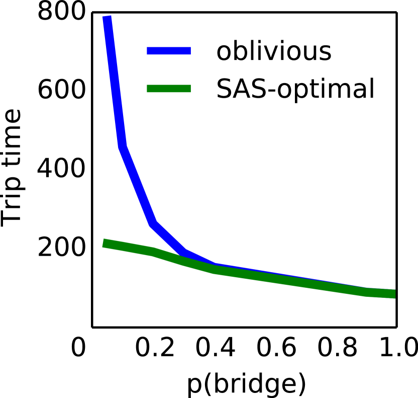
We now provide a somewhat more elaborate empirical demonstration of the effects of stochastic action availability. Consider an MDP that corresponds to a routing problem on a real-world road network (Fig.Β 1) in the San Francisco Bay Area. The shortest path between the source and destination locations is sought. The dashed edge in Fig.Β 1 represents a bridge, available only with probability $p$, while all other edges correspond to action choices available with probability $0.5$. At each node, a no-op action (waiting) is available at constant cost; otherwise the edge costs are the geodesic lengths of the corresponding roads on the map. The optimal policies for different choices $p=0.1,0.2$ and $0.4$ are depicted in Fig.Β 1, where line thickness and color indicate traversal probabilities under the corresponding optimal policies. It can be observed that lower values of $p$ lead to policies with more redundancy. Fig.Β 2 investigates the effect of solving the routing problem obliviously to the stochastic action availability (assuming actions are fully available). The SAS-optimal policy allows graceful scaling of the expected travel time from source to destination as bridge availability decreases. Finalluy, the effects of violating the PDA assumption are investigated in the long version of this workΒ [TODO].

Refer to caption
Figure 1: Stochastic action MDPs applied to routing.
Refer to caption
Figure 2: Expected trip time from source to destination under the SAS-optimal policy vs. under the oblivious optimal policy (the MDP solved as if actions are fully available) as a function of bridge availability.

9 Concluding Remarks

We have developed a new MDP model, SAS-MDPs, that extends the usual finite-action MDP model by allowing the set of available actions to vary stochastically. This captures an important use case that arises in many practical applications (e.g., online advertising, recommender systems). We have shown that embedding action sets in the state gives a standard MDP, supporting tractable analysis at the cost of an exponential blow-up in state space size. Despite this, we demonstrated that (optimal and greedy) policies have a useful decision list structure. We showed how this DL format can be exploited to construct tractable Q-learning, value and policy iteration, and linear programming algorithms.

While our work offers firm foundations for stochastic action sets, most practical applications will not use the algorithms described here explicitly. For example, in RL, we generally use function approximators for generalization and scalability in large state/action problems. We have successfully applied Q-learning using DNN function approximators (i.e.,Β DQN) using sampled/logged available actions in ads and recommendations domains as described in Sec.Β 4. This has allowed us to apply SAS-Q-learning to problems of significant, commercially viable scale. Model-based methods such as VI, PI, and LP also require suitable (e.g., factored) representations of MDPs and structured implementations of our algorithms that exploit these representations. For instance, extensions of approximate linear programming or structured dynamic programming to incorporate stochastic action sets would be extremely valuable.

Other important questions include developing a polynomial-sized direct LP formulation; and deriving sample-complexity results for RL algorithms like Q-learning is also of particular interest, especially as it pertains to the sampling of the action distribution. Finally, we are quite interested in relaxing the strong assumptions embodied in the PDA modelβ€”of particular interest is the extension of our algorithms to less extreme forms of action availability independence, for example, as represented using consise graphical models (e.g., Bayes nets).

Acknowledgments: Thanks to the reviewers for their helpful suggestions.

References

  • [1] Shortest paths without a map. Theoretical Computer Science, 84(1):127 – 150, 1991.
  • [2] Kareem Amin, Michael Kearns, Peter Key, and Anton Schwaighofer. Budget optimization for sponsored search: Censored learning in MDPs. In Proceedings of the Twenty-eighth Conference on Uncertainty in Artificial Intelligence (UAI-12), pages 543–553, Catalina, CA, 2012.
  • [3] Nikolay Archak, Vahab Mirrokni, and S.Β Muthukrishnan. Budget optimization for online campaigns with positive carryover effects. In Proceedings of the Eighth International Workshop on Internet and Network Economics (WINE-12), pages 86–99, Liverpool, 2012.
  • [4] Nikolay Archak, VahabΒ S. Mirrokni, and S.Β Muthukrishnan. Mining advertiser-specific user behavior using adfactors. In Proceedings of the Nineteenth International World Wide Web Conference (WWW 2010), pages 31–40, Raleigh, NC, 2010.
  • [5] Craig Boutilier, Alon Cohen, Avinatan Hassidim, Yishay Mansour, Ofer Meshi, Martin Mladenov, and Dale Schuurmans. Planning and learning in Markov decision processes with stochastic action sets. arXiv:1805.02363, 2018.
  • [6] Moses Charikar, Ravi Kumar, Prabhakar Raghavan, Sridhar Rajagopalan, and Andrew Tomkins. On targeting Markov segments. In Proceedings of the 31st Annual ACM Symposium on Theory of Computing (STOC-99), pages 99–108, Atlanta, 1999.
  • [7] Martin GrΓΆtschel, LΓ‘szlo LovΓ‘sz, and Alexander Schrijver. Geometric Algorithms and Combinatorial Optimization, volumeΒ 2 of Algorithms and Combinatorics. Springer, 1988.
  • [8] ThomasΒ Dueholm Hansen, PeterΒ Bro Miltersen, and Uri Zwick. Strategy iteration is strongly polynomial for 2-player turn-based stochastic games with a constant discount factor. Journal of the ACM (JACM), 60(1), 2013. Article 1, 16pp.
  • [9] Varun Kanade, HΒ Brendan McMahan, and Brent Bryan. Sleeping experts and bandits with stochastic action availability and adversarial rewards. In Twelfth International Conference on Artificial Intelligence and Statistics (AIStats-09), pages 272–279, Clearwater Beach, FL, 2009.
  • [10] Robert Kleinberg, Alexandru Niculescu-Mizil, and Yogeshwer Sharma. Regret bounds for sleeping experts and bandits. Machine learning, 80(2–3):245–272, 2010.
  • [11] Ting Li, Ning Liu, Jun Yan, Gang Wang, Fengshan Bai, and Zheng Chen. A Markov chain model for integrating behavioral targeting into contextual advertising. In Proceedings of the Third International Workshop on Data Mining and Audience Intelligence for Advertising (ADKDD-09), pages 1–9, Paris, 2009.
  • [12] U.Β Meister and U.Β Holzbaur. A polynomial time bound for Howard’s policy improvement algorithm. OR Spektrum, 8:37–40, 1986.
  • [13] Martin Mladenov, Craig Boutilier, Dale Schuurmans, Ofer Meshi, Gal Elidan, and Tyler Lu. Logistic Markov decision processes. In Proceedings of the Twenty-sixth International Joint Conference on Artificial Intelligence (IJCAI-17), pages 2486–2493, Melbourne, 2017.
  • [14] Volodymyr Mnih, Koray Kavukcuoglu, David Silver, Alex Graves, Ioannis Antonoglou, Daan Wierstra, and Martin Riedmiller. Playing Atari with deep reinforcement learning. arXiv preprint arXiv:1312.5602, 2013.
  • [15] Volodymyr Mnih, Koray Kavukcuoglu, David Silver, AndreiΒ A Rusu, Joel Veness, MarcΒ G Bellemare, Alex Graves, Martin Riedmiller, AndreasΒ K Fidjeland, Georg Ostrovski, etΒ al. Human-level control through deep reinforcement learning. Nature, 518(7540):529–533, 2015.
  • [16] Evdokia Nikolova and DavidΒ R. Karger. Route planning under uncertainty: The Canadian traveller problem. In Proceedings of the 23rd National Conference on Artificial Intelligence - Volume 2, AAAI’08, pages 969–974. AAAI Press, 2008.
  • [17] GeorgeΒ H. Polychronopoulos and JohnΒ N. Tsitsiklis. Stochastic shortest path problems with recourse. Networks, 27(2).
  • [18] MartinΒ L. Puterman. Markov Decision Processes: Discrete Stochastic Dynamic Programming. Wiley, New York, 1994.
  • [19] David Silver, Leonard Newnham, David Barker, Suzanne Weller, and Jason McFall. Concurrent reinforcement learning from customer interactions. In Proceedings of the 30th International Conference on Machine Learning (ICML-13), pages 924–932, Atlanta, 2013.
  • [20] Georgios Theocharous, PhilipΒ S. Thomas, and Mohammad Ghavamzadeh. Personalized ad recommendation systems for life-time value optimization with guarantees. In Proceedings of the Twenty-fourth International Joint Conference on Artificial Intelligence (IJCAI-15), pages 1806–1812, Buenos Aires, 2015.
  • [21] Paul Tseng. Solving h-horizon, stationary Markov decision problems in time proportional to log(h). Operations Research Letters, 9(5):287–297, 1990.
  • [22] Christopher J. C.Β H. Watkins and Peter Dayan. Q-learning. Machine Learning, 8:279–292, 1992.
  • [23] Yinyu Ye. The simplex and policy-iteration methods are strongly polynomial for the Markov decision problem with a fixed discount rate. Mathematics of Operations Research, 36(4):593–603, 2011.

Appendix A Proofs

A.1 Proof of LemmaΒ 1

$\displaystyle ET^{e}V_{e}(s)$ $\displaystyle=\mathop{\mathbb{E}}_{A\subseteq B}T^{e}V_{e}(s\circ A)$
=𝔼AβŠ†Bmaxk∈A⁑rsk+Ξ³β€‹βˆ‘sβ€²βˆ˜Aβ€²ps∘A,sβ€²βˆ˜Aβ€²k​Ve​(sβ€²βˆ˜Aβ€²)absentsubscript𝔼𝐴𝐡subscriptπ‘˜π΄subscriptsuperscriptπ‘Ÿπ‘˜π‘ π›Ύsubscriptsuperscript𝑠′superscript𝐴′subscriptsuperscriptπ‘π‘˜π‘ π΄superscript𝑠′superscript𝐴′subscript𝑉𝑒superscript𝑠′superscript𝐴′\displaystyle=\mathop{\mathbb{E}}_{A\subseteq B}\max_{k\in A}r^{k}_{s}+\gamma\sum_{s^{\prime}\circ A^{\prime}}p^{k}_{s\circ A,s^{\prime}\circ A^{\prime}}V_{e}(s^{\prime}\circ A^{\prime})
=𝔼AβŠ†Bmaxk∈A⁑rsk+Ξ³β€‹βˆ‘sβ€²ps,sβ€²k​𝔼Aβ€²βŠ†BVe​(sβ€²βˆ˜Aβ€²)absentsubscript𝔼𝐴𝐡subscriptπ‘˜π΄subscriptsuperscriptπ‘Ÿπ‘˜π‘ π›Ύsubscriptsuperscript𝑠′subscriptsuperscriptπ‘π‘˜π‘ superscript𝑠′subscript𝔼superscript𝐴′𝐡subscript𝑉𝑒superscript𝑠′superscript𝐴′\displaystyle=\mathop{\mathbb{E}}_{A\subseteq B}\max_{k\in A}r^{k}_{s}+\gamma\sum_{s^{\prime}}p^{k}_{s,s^{\prime}}\mathop{\mathbb{E}}_{A^{\prime}\subseteq B}V_{e}(s^{\prime}\circ A^{\prime})
=𝔼AβŠ†Bmaxk∈A⁑rsk+Ξ³β€‹βˆ‘sβ€²ps,sβ€²k​E​Ve​(sβ€²)absentsubscript𝔼𝐴𝐡subscriptπ‘˜π΄subscriptsuperscriptπ‘Ÿπ‘˜π‘ π›Ύsubscriptsuperscript𝑠′subscriptsuperscriptπ‘π‘˜π‘ superscript𝑠′𝐸superscript𝑉𝑒superscript𝑠′\displaystyle=\mathop{\mathbb{E}}_{A\subseteq B}\max_{k\in A}r^{k}_{s}+\gamma\sum_{s^{\prime}}p^{k}_{s,s^{\prime}}EV^{e}(s^{\prime})
$\displaystyle=T^{c}EV^{e}(s^{\prime}).$

A.2 Proof of LemmaΒ 2

It is easy to compute the expected value of each action in $k\in A$ using a one-step backup of $V^{\ast}_{c}$. The action with maximum value is Ο€eβˆ—β€‹(s∘A)subscriptsuperscriptπœ‹βˆ—π‘’π‘ π΄\pi^{\ast}_{e}(s\circ A) and its backed-up expected value is Veβˆ—β€‹(s∘A)subscriptsuperscriptπ‘‰βˆ—π‘’π‘ π΄V^{\ast}_{e}(s\circ A).

A.3 Proof of LemmaΒ 3

Since $\mathcal{M}_{e}$ is a standard MDP, we know $\mathcal{M}_{e}$ is a contraction with modulus $\gamma$. Let $v_{c}=Ev_{e}$ and $v_{c}^{\prime}=Ev^{\prime}_{e}$ be compressed value functions that each correspond to some (arbitrary) embedded value function. Then for any $s$ we have:

$\displaystyle|T^{c}v_{c}(s)-T^{c}v^{\prime}_{c}(s)|$ $\displaystyle=|\mathop{\mathbb{E}}_{A\subseteq B}T^{e}v_{e}(s\circ A)-\mathop{\mathbb{E}}_{A\subseteq B}T^{e}v^{\prime}_{e}(s\circ A)|$
$\displaystyle=|\mathop{\mathbb{E}}_{A\subseteq B}(T^{e}v_{e}(s\circ A)-T^{e}v^{\prime}_{e}(s\circ A)|$
$\displaystyle\leq|\mathop{\mathbb{E}}_{A\subseteq B}\gamma(v_{e}(s\circ A)-v^{\prime}_{e}(s\circ A)|$
$\displaystyle=\gamma|\mathop{\mathbb{E}}_{A\subseteq B}v_{e}(s\circ A)-\mathop{\mathbb{E}}_{A\subseteq B}v^{\prime}_{e}(s\circ A)|$
$\displaystyle=\gamma|v_{c}(s)-v^{\prime}_{c}(s)|.$

Appendix B Guarantees on the ADS Assumption

Let μ​(s)​(A)πœ‡π‘ π΄\mu(s)(A) be the top action according to the DL μ​(s)πœ‡π‘ \mu(s). We have the following theorem, which is a direct application of Hoeffding’s concentration inequality along with a union bound.

Lemma 4

Let $Q^{\star}$ be optimal for the MDP. Suppose that for each state $s$ we sample $A_{s}^{(1)},\ldots,A_{s}^{(t)}$. If

$$m=\Omega\left(\left(\frac{\gamma}{1-\gamma}\right)^{2}\frac{|A|+\log(|S|/\delta)}{\epsilon^{2}}\right)~{},$$

then with probability $1-\delta$, for each DL policy $\mu$ we have

|𝔼AβŠ†BQμ​(s,μ​(s)​(A))βˆ’1Tβ€‹βˆ‘t=1TQμ​(s,μ​(s)​(As(t)))|≀ϡ​(1βˆ’Ξ³)2​γ.subscript𝔼𝐴𝐡superscriptπ‘„πœ‡π‘ πœ‡π‘ π΄1𝑇superscriptsubscript𝑑1𝑇superscriptπ‘„πœ‡π‘ πœ‡π‘ superscriptsubscript𝐴𝑠𝑑italic-Ο΅1𝛾2𝛾\left|\mathop{\mathbb{E}}_{A\subseteq B}Q^{\mu}(s,\mu(s)(A))-\frac{1}{T}\sum_{t=1}^{T}Q^{\mu}(s,\mu(s)(A_{s}^{(t)}))\right|\leq\frac{\epsilon(1-\gamma)}{2\gamma}~{}.

We can use the lemma above to approximate the $Q$ function by the one corresponding to an approximate-MDP, resulted by the sub-sampling of the action subsets.

Lemma 5

Let $\widehat{Q}^{\mu}$ be the $Q$ function corresponding to policy $\mu$ for the approximate-MDP. Then, for any policy $\mu$, state $s$ and action $a$,

|Qμ​(s,a)βˆ’Q^μ​(s,a)|≀ϡ2.superscriptπ‘„πœ‡π‘ π‘Žsuperscript^π‘„πœ‡π‘ π‘Žitalic-Ο΅2\left|Q^{\mu}(s,a)-\widehat{Q}^{\mu}(s,a)\right|\leq\frac{\epsilon}{2}~{}.
Proof.

We will show one direction of the proof, and the other will follow by a symmetric argument. Let us unfold the $Q$ function by successive applications of LemmaΒ 4,

Qμ​(s,a)superscriptπ‘„πœ‡π‘ π‘Ž\displaystyle Q^{\mu}(s,a) =𝔼sβ€²|s,a[r​(s,a)+γ​𝔼AβŠ†BQμ​(sβ€²,μ​(sβ€²)​(A))]absentsubscript𝔼conditionalsuperscriptπ‘ β€²π‘ π‘Ždelimited-[]π‘Ÿπ‘ π‘Žπ›Ύsubscript𝔼𝐴𝐡superscriptπ‘„πœ‡superscriptπ‘ β€²πœ‡superscript𝑠′𝐴\displaystyle=\mathop{\mathbb{E}}_{s^{\prime}|s,a}\left[r(s,a)+\gamma\mathop{\mathbb{E}}_{A\subseteq B}Q^{\mu}(s^{\prime},\mu(s^{\prime})(A))\right]
≀𝔼sβ€²|s,a[r​(s,a)+Ξ³β‹…1Tβ€‹βˆ‘t=1T(Qμ​(sβ€²,μ​(sβ€²)​(Asβ€²(t)))+ϡ​(1βˆ’Ξ³)2​γ)]absentsubscript𝔼conditionalsuperscriptπ‘ β€²π‘ π‘Ždelimited-[]π‘Ÿπ‘ π‘Žβ‹…π›Ύ1𝑇superscriptsubscript𝑑1𝑇superscriptπ‘„πœ‡superscriptπ‘ β€²πœ‡superscript𝑠′superscriptsubscript𝐴superscript𝑠′𝑑italic-Ο΅1𝛾2𝛾\displaystyle\leq\mathop{\mathbb{E}}_{s^{\prime}|s,a}\left[r(s,a)+\gamma\cdot\frac{1}{T}\sum_{t=1}^{T}\left(Q^{\mu}(s^{\prime},\mu(s^{\prime})(A_{s^{\prime}}^{(t)}))+\frac{\epsilon(1-\gamma)}{2\gamma}\right)\right]
=𝔼sβ€²|s,a[r​(s,a)+Ξ³Tβ€‹βˆ‘t=1TQμ​(sβ€²,μ​(sβ€²)​(Asβ€²(t)))]+ϡ​(1βˆ’Ξ³)2.absentsubscript𝔼conditionalsuperscriptπ‘ β€²π‘ π‘Ždelimited-[]π‘Ÿπ‘ π‘Žπ›Ύπ‘‡superscriptsubscript𝑑1𝑇superscriptπ‘„πœ‡superscriptπ‘ β€²πœ‡superscript𝑠′superscriptsubscript𝐴superscript𝑠′𝑑italic-Ο΅1𝛾2\displaystyle=\mathop{\mathbb{E}}_{s^{\prime}|s,a}\left[r(s,a)+\frac{\gamma}{T}\sum_{t=1}^{T}Q^{\mu}(s^{\prime},\mu(s^{\prime})(A_{s^{\prime}}^{(t)}))\right]+\frac{\epsilon(1-\gamma)}{2}~{}.

Repeating the argument above with respect to Qμ​(sβ€²,μ​(sβ€²)​(Asβ€²(t)))superscriptπ‘„πœ‡superscriptπ‘ β€²πœ‡superscript𝑠′superscriptsubscript𝐴superscript𝑠′𝑑Q^{\mu}(s^{\prime},\mu(s^{\prime})(A_{s^{\prime}}^{(t)})) and continuing so recursively, we obtain

Qμ​(s,a)≀Q^μ​(s,a)+βˆ‘t=0∞γt​ϡ​(1βˆ’Ξ³)2=Q^μ​(s,a)+Ο΅2.superscriptπ‘„πœ‡π‘ π‘Žsuperscript^π‘„πœ‡π‘ π‘Žsuperscriptsubscript𝑑0superscript𝛾𝑑italic-Ο΅1𝛾2superscript^π‘„πœ‡π‘ π‘Žitalic-Ο΅2Q^{\mu}(s,a)\leq\widehat{Q}^{\mu}(s,a)+\sum_{t=0}^{\infty}\gamma^{t}\frac{\epsilon(1-\gamma)}{2}=\widehat{Q}^{\mu}(s,a)+\frac{\epsilon}{2}~{}.

∎

We can now state our theorem.

Theorem 6

Let $\hat{\mu}$ be the optimal policy for the approximate-MDP. For each state $s$ and action $a$, QΞΌ^​(s,a)β‰₯Q⋆​(s,a)βˆ’Ο΅superscript𝑄^πœ‡π‘ π‘Žsuperscriptπ‘„β‹†π‘ π‘Žitalic-Ο΅Q^{\hat{\mu}}(s,a)\geq Q^{\star}(s,a)-\epsilon.

Proof.

We have,

Q⋆​(s,a)superscriptπ‘„β‹†π‘ π‘Ž\displaystyle Q^{\star}(s,a) ≀Q^μ⋆​(s,a)+Ο΅2absentsuperscript^𝑄superscriptπœ‡β‹†π‘ π‘Žitalic-Ο΅2\displaystyle\leq\widehat{Q}^{\mu^{\star}}(s,a)+\frac{\epsilon}{2} (LemmaΒ 5)
≀Q^ΞΌ^​(s,a)+Ο΅2absentsuperscript^𝑄^πœ‡π‘ π‘Žitalic-Ο΅2\displaystyle\leq\widehat{Q}^{\hat{\mu}}(s,a)+\frac{\epsilon}{2} ($\hat{\mu}$ optimal for $\widehat{Q}$)
≀QΞΌ^​(s,a)+Ο΅.absentsuperscript𝑄^πœ‡π‘ π‘Žitalic-Ο΅\displaystyle\leq Q^{\hat{\mu}}(s,a)+\epsilon~{}. (LemmaΒ 5)

∎

Appendix C Non-stochastic Action Availability

Suppose that the action subsets are chosen by an adversarial process, yet are known in advance. In this case the optimal policy might neither be stationary nor a decision list. This is shown in the following example.

$1$ $2$ $3$ $a$ $b$ $c$

Consider the MDP drawn above, which has three states. When the agent is at state 1, she has the choice of playing actions $a$, $b$ or $c$. Actions $b$ and $c$ are always available, and $b$ generates a slightly higher reward than $c$666Compared to the discounting factor.. Action $a$ is available once in a while, and its reward is much higher than both $b$ and $c$.

When the agent visits state 1 and action $a$ is unavailable, she will usually prefer playing action $b$. However, should the agent know that action $a$ will become available in the next turn, she will play action $c$. This is even though in both cases the set of available actions is the same!

Appendix D The Complexity of Value Iteration

Given its polytime per-iteration complexity, to ensure VI is polytime, we must show that it converges to a value function that induces an optimal policy in a polynomially many iterations. To do so, we exploit the compressed representation and adapt the technique of [21].

First we need some assumptions and definitions w.r.t.Β the base MDP $\mathcal{M}$:

  • β€’

    Assume (w.l.o.g.) that all rewards/costs are integers.

  • β€’

    Let $\delta$ be the smallest integer s.t. $\delta\gamma$ and δ​ps,sβ€²k𝛿subscriptsuperscriptπ‘π‘˜π‘ superscript𝑠′\delta p^{k}_{s,s^{\prime}} (for all actions, states) are integer and Ξ΄>rsk𝛿subscriptsuperscriptπ‘Ÿπ‘˜π‘ \delta>r^{k}_{s} for all states, actions. This is the precision needed to represent the base: each parameter requires $\log\delta$ bits.

Tseng shows that VI for a standard MDP is weakly polynomial (assuming a constant discount factor $\gamma$), by proving that: (a) if the $t$th value function produced by VI satisfies

$$||V^{t}-V^{\ast}||<1/(2\delta^{2n+2}n^{n}),$$

then the policy induced by $V^{t}$ is optimal; and (b) VI achieves this bound in polynomially many iterations.

Tseng’s proof involves several steps:

  • β€’

    A simple argument based on the precision of the parameters shows that for all $s$, Vβˆ—β€‹(s)=ws/(Ξ΄2​n​nn)superscriptπ‘‰βˆ—π‘ subscript𝑀𝑠superscript𝛿2𝑛superscript𝑛𝑛V^{\ast}(s)=w_{s}/(\delta^{2n}n^{n}) for some integer $w_{s}$: Let $\mu$ be any policy. Then the induced transition matrix $P^{\mu}$ and the immediate reward vector $R^{\mu}$ are such that $Z=\delta^{2}(I-\gamma P^{\mu})$ and $\delta^{2}R^{\mu}$ are integral (and the entries of $Z$ are less than $\delta^{2}$). Then for the optimal policy $\mu$, by Cramer’s rule we have that Vβˆ—β€‹(s)=detZs/detZsuperscriptπ‘‰βˆ—π‘ subscript𝑍𝑠𝑍V^{\ast}(s)=\det Z_{s}/\det Z (where $Z_{s}$ is $Z$ with $R^{\mu}$ replacing column $s$). By Hadamard’s inequality, the determinant of $Z$ is bounded by $\delta^{2n}n^{n/2}$, and since the determinant of $Z_{s}$ must also be integral, the stated fact follows.

  • β€’

    An action elimination argument based on the precision of the solution shows that the action backup of any nonoptimal action w.r.t.Β Vβˆ—superscriptπ‘‰βˆ—V^{\ast} must differ from that of the optimal action by at least $1/(\delta^{2n+2}n^{n})$: Suppose action $k$ is not optimal at $s$, hence Qβˆ—β€‹(s,k)=Tk​Vβˆ—β€‹(s)<Tμ​Vβˆ—β€‹(s)superscriptπ‘„π‘ π‘˜superscriptπ‘‡π‘˜superscriptπ‘‰βˆ—π‘ superscriptπ‘‡πœ‡superscriptπ‘‰βˆ—π‘ Q^{*}(s,k)=T^{k}V^{\ast}(s)<T^{\mu}V^{\ast}(s) (where $\mu$ is the optimal policy). Then

    Tk​Vβˆ—β€‹(s)superscriptπ‘‡π‘˜superscriptπ‘‰βˆ—π‘ \displaystyle T^{k}V^{\ast}(s) =Ξ³β€‹βˆ‘sβ€²ps​sβ€²k​Vβˆ—β€‹(s)+rskabsent𝛾subscriptsuperscript𝑠′subscriptsuperscriptπ‘π‘˜π‘ superscript𝑠′superscriptπ‘‰βˆ—π‘ subscriptsuperscriptπ‘Ÿπ‘˜π‘ \displaystyle=\gamma\sum_{s^{\prime}}p^{k}_{ss^{\prime}}V^{\ast}(s)+r^{k}_{s}
    =Ξ³β€‹βˆ‘sβ€²ps​sβ€²k​ws/(Ξ΄2​n​nn)+rskabsent𝛾subscriptsuperscript𝑠′subscriptsuperscriptπ‘π‘˜π‘ superscript𝑠′subscript𝑀𝑠superscript𝛿2𝑛superscript𝑛𝑛subscriptsuperscriptπ‘Ÿπ‘˜π‘ \displaystyle=\gamma\sum_{s^{\prime}}p^{k}_{ss^{\prime}}w_{s}/(\delta^{2n}n^{n})+r^{k}_{s}
    =Ξ΄2β€‹Ξ³β€‹βˆ‘sβ€²ps​sβ€²k​ws+Ξ΄2​n+2​nn/2​rskΞ΄2​n+2​nn.absentsuperscript𝛿2𝛾subscriptsuperscript𝑠′subscriptsuperscriptπ‘π‘˜π‘ superscript𝑠′subscript𝑀𝑠superscript𝛿2𝑛2superscript𝑛𝑛2subscriptsuperscriptπ‘Ÿπ‘˜π‘ superscript𝛿2𝑛2superscript𝑛𝑛\displaystyle=\frac{\delta^{2}\gamma\sum_{s^{\prime}}p^{k}_{ss^{\prime}}w_{s}+\delta^{2n+2}n^{n/2}r^{k}_{s}}{\delta^{2n+2}n^{n}}.

    Since the numerator is integral (and so is $w_{s}$), Tk​Vβˆ—β€‹(s)superscriptπ‘‡π‘˜superscriptπ‘‰βˆ—π‘ T^{k}V^{\ast}(s) and Tcμ​Vβˆ—β€‹(s)subscriptsuperscriptπ‘‡πœ‡π‘superscriptπ‘‰βˆ—π‘ T^{\mu}_{c}V^{\ast}(s) must differ by at least $1/(\delta^{2n}n^{n})$. Thus if $||V^{t}-v^{\ast}||<1/(2\delta^{2n}n^{n})$ (where $V^{t}$ is $t$th iterate of VI), some simple substitutions show that the policy induced by $V^{t}$ must be optimal.

  • β€’

    For any target precision $\varepsilon$, Tseng uses standard arguments to show that after $t$ iterations, the error $||V^{t}-v^{\ast}||<\varepsilon$, where $t=\lceil\log(||V^{\ast}||/(1-\gamma)\varepsilon)/\log(1/\gamma)\rceil$. We can plug in the usual upper bound $U$ on $V^{\ast}$, which is $U=r_{\max}/(1-\gamma)=O(r_{\max})$ for a fixed $\gamma$.

  • β€’

    Substituting the precision $1/(2\delta^{2n}n^{n})$ for $\varepsilon$ gives a polytime bound on required iterations:

    $$t^{*}\leq\log(2\delta^{2n}n^{n}U)/\log(1/\gamma).$$

We derive a similar bound on the number of VI iterations needed for convergence in an SAS-MDP, using the same input parameters as in the base MDP, and applying the the same precision $\delta$ to the action availability probabilities. We apply Tseng’s result by exploiting the fact that: (a) the optimal policy for the embedded MDP $\mathcal{M}_{e}$ can be represented as a DL; (b) the transition function for any DL policy can be expressed using an $n\times n$ matrix (we simply take expectations, see above); and (c) the corresponding linear system can be expressed over the compressed rather than the embedded state space to determine $V_{c}^{\ast}$ (rather than $V_{e}^{\ast}$).

Tseng’s argument requires some adaptation to apply to the compressed VI algorithm. His definition of $\delta$ ensures that the terms in the linear system when multiplied by $\delta^{2}$ are integers, which in turn ensures the solution for $V^{\ast}$ has precision limited to $\delta^{2n}n^{n}$. We extend his precision assumption to account for our action availability probabilities as well, ensuring δ​ρsk𝛿subscriptsuperscriptπœŒπ‘˜π‘ \delta\rho^{k}_{s} is integral for all s∈S,k∈Bformulae-sequenceπ‘ π‘†π‘˜π΅s\in S,k\in B.

Since $\mathcal{M}_{c}$ is an MDP, Tseng’s result applies; but notice that the transition matrix for any state’s DL $\mu$, which serves as an action in $\mathcal{M}_{c}$, has entries of the form:

ps,sβ€²ΞΌ=βˆ‘i=1m[∏j=1iβˆ’1(1βˆ’Οsμ​(s)​(j))]​ρsμ​(s)​(i)​ps,s′μ​(s)​(i).subscriptsuperscriptπ‘πœ‡π‘ superscript𝑠′superscriptsubscript𝑖1π‘šdelimited-[]superscriptsubscriptproduct𝑗1𝑖11subscriptsuperscriptπœŒπœ‡π‘ π‘—π‘ subscriptsuperscriptπœŒπœ‡π‘ π‘–π‘ subscriptsuperscriptπ‘πœ‡π‘ π‘–π‘ superscript𝑠′p^{\mu}_{s,s^{\prime}}=\sum_{i=1}^{m}\,[\prod_{j=1}^{i-1}(1-\rho^{\mu(s)(j)}_{s})]\,\rho^{\mu(s)(i)}_{s}p^{\mu(s)(i)}_{s,s^{\prime}}.

Since this is the product of $m+1$ probabilities, each with precision $\delta$, we have that Ξ΄m+1​ps,sβ€²ΞΌsuperscriptπ›Ώπ‘š1subscriptsuperscriptπ‘πœ‡π‘ superscript𝑠′\delta^{m+1}p^{\mu}_{s,s^{\prime}} must also be integer. Thus the required precision parameter for our MDP is at most $\delta^{m+1}$. Plugging this into Tseng’s bound, VI applied to $\mathcal{M}_{c}$ must induce an optimal policy at the $t$th iteration if

$$||V^{t}-v^{\ast}||<1/(2\delta^{(m+1)^{2n}}n^{n})=1/(2\delta^{(m+1)2n}n^{n}).$$

This in turn gives us a bound on the number of iterations of VI needed to reach an optimal policy:

Theorem 7

VI applied to $\mathcal{M}_{c}$ converges to a value function whose greedy policy is optimal in $t*$ iterations, where

$$t^{*}\leq\log(2\delta^{2n(m+1)}n^{n}M)/\log(1/\gamma).$$

Combined with Obs.Β 1, we have:

Corollary 3

VI yields an optimal policy for the SAS-MDP corresponding to $\mathcal{M}_{c}$ in polynomial time.

We remark that in the ADS model, we only obtain an approximation to the optimal policy. In fact, one cannot compute an exact optimal policy without observing the entire support of the availability distributions, which requires an exponential sample size.

Under the product distribution assumption, the theorem particularly implies that the convergence of policy iteration in strongly-polynomial time as long as each of the actions is available with constant probability. In this case, for any Ο€,ai,aj,sπœ‹subscriptπ‘Žπ‘–subscriptπ‘Žπ‘—π‘ \pi,a_{i},a_{j},s we have ηπ​(s,ai,aj)β‰₯pi​pj=Ω​(1)subscriptπœ‚πœ‹π‘ subscriptπ‘Žπ‘–subscriptπ‘Žπ‘—subscript𝑝𝑖subscript𝑝𝑗Ω1\eta_{\pi}(s,a_{i},a_{j})\geq p_{i}p_{j}=\Omega(1), which in turn implies that we can take $q$ to be $\Omega(1)$ in the bound above.

Appendix E The Complexity of Policy Iteration

This is an adaptation of the Hansen, Miltersen, Zwick paper.

E.1 Policy Iteration

Let $\mu(A|s)$ be the probability of having available actions $A$ in state $s$. Denote $\sigma$ to be a permutation of the actions, and $\sigma(A)$ is the first available action in $A$ according to $\sigma$. Also denote ηπ​(s,a1,a2)=μ​{A:π⋆​(s)​(A)=a1,π​(s)​(A)=a2|s}subscriptπœ‚πœ‹π‘ subscriptπ‘Ž1subscriptπ‘Ž2πœ‡conditional-set𝐴formulae-sequencesuperscriptπœ‹β‹†π‘ π΄subscriptπ‘Ž1πœ‹π‘ π΄conditionalsubscriptπ‘Ž2𝑠\eta_{\pi}(s,a_{1},a_{2})=\mu\{A:\pi^{\star}(s)(A)=a_{1},\pi(s)(A)=a_{2}|s\}, the probability that $\pi^{\star}$ plays $a_{1}$ and simultaneously $\pi$ plays $a_{2}$.

Algorithm 1 Policy Iteration
Β Β Initialize: $\pi_{1}$
Β Β forΒ t=1,2,…𝑑12…t=1,2,\ldotsΒ do
Β Β Β Β Β Compute: VΟ€t=𝔼A|s[r​(s,Ο€t​(s)​(A))+γ​𝔼sβ€²|s,Ο€t​(s)​(A)VΟ€t​(sβ€²)]superscript𝑉subscriptπœ‹π‘‘subscript𝔼conditional𝐴𝑠delimited-[]π‘Ÿπ‘ subscriptπœ‹π‘‘π‘ π΄π›Ύsubscript𝔼conditionalsuperscript𝑠′𝑠subscriptπœ‹π‘‘π‘ π΄superscript𝑉subscriptπœ‹π‘‘superscript𝑠′V^{\pi_{t}}=\mathop{\mathbb{E}}_{A|s}\left[r(s,\pi_{t}(s)(A))+\gamma\mathop{\mathbb{E}}_{s^{\prime}|s,\pi_{t}(s)(A)}V^{\pi_{t}}(s^{\prime})\right]
Β Β Β Β Β Update: Ο€t+1​(s)=arg​maxσ​𝔼A|s[r​(s,σ​(A))+γ​𝔼sβ€²|s,σ​(A)VΟ€t​(sβ€²)]subscriptπœ‹π‘‘1𝑠subscriptargmax𝜎subscript𝔼conditional𝐴𝑠delimited-[]π‘Ÿπ‘ πœŽπ΄π›Ύsubscript𝔼conditionalsuperscriptπ‘ β€²π‘ πœŽπ΄superscript𝑉subscriptπœ‹π‘‘superscript𝑠′\pi_{t+1}(s)=\operatorname*{arg\,max}_{\sigma}\mathop{\mathbb{E}}_{A|s}\left[r(s,\sigma(A))+\gamma\mathop{\mathbb{E}}_{s^{\prime}|s,\sigma(A)}V^{\pi_{t}}(s^{\prime})\right]
Β Β endΒ for
Theorem 8

$\|V^{\pi_{t+1}}-V^{\star}\|\leq\gamma\|V^{\pi_{t}}-V^{\star}\|$.

Proof.

For any $s$,

$\displaystyle V^{\star}(s)-V^{\pi_{t+1}}(s)$ ≀γ​maxσ​𝔼A|s𝔼s|sβ€²,σ​(A)(V⋆​(sβ€²)βˆ’VΟ€t​(sβ€²))absent𝛾subscript𝜎subscript𝔼conditional𝐴𝑠subscript𝔼conditional𝑠superscriptπ‘ β€²πœŽπ΄superscript𝑉⋆superscript𝑠′superscript𝑉subscriptπœ‹π‘‘superscript𝑠′\displaystyle\leq\gamma\max_{\sigma}\mathop{\mathbb{E}}_{A|s}\mathop{\mathbb{E}}_{s|s^{\prime},\sigma(A)}\left(V^{\star}(s^{\prime})-V^{\pi_{t}}(s^{\prime})\right)
$\displaystyle\leq\gamma\|V^{\pi_{t}}-V^{\star}\|~{}.$

∎

E.2 Polynomial bound

In this section we will prove the following theorem.

Theorem 9

Assume there exists $q>0$ such that for any policy $\pi$, state $s$ and actions $a_{1},a_{2}$, ηπ​(s,a1,a2)>0subscriptπœ‚πœ‹π‘ subscriptπ‘Ž1subscriptπ‘Ž20\eta_{\pi}(s,a_{1},a_{2})>0 implies ηπ​(s,a1,a2)β‰₯qsubscriptπœ‚πœ‹π‘ subscriptπ‘Ž1subscriptπ‘Ž2π‘ž\eta_{\pi}(s,a_{1},a_{2})\geq q. Then policy iteration converges after

$$O\left(\frac{|S||A|^{2}}{1-\gamma}\log\frac{|A|}{1-\gamma}\left(1+\log\frac{1}{q}\right)\right)$$

iterations.

Under the product distribution assumption, the theorem particularly implies that the convergence of policy iteration in strongly-polynomial time as long as each of the actions is available with constant probability. In this case, for any Ο€,ai,aj,sπœ‹subscriptπ‘Žπ‘–subscriptπ‘Žπ‘—π‘ \pi,a_{i},a_{j},s we have ηπ​(s,ai,aj)β‰₯pi​pj=Ω​(1)subscriptπœ‚πœ‹π‘ subscriptπ‘Žπ‘–subscriptπ‘Žπ‘—subscript𝑝𝑖subscript𝑝𝑗Ω1\eta_{\pi}(s,a_{i},a_{j})\geq p_{i}p_{j}=\Omega(1), which in turn implies that we can take $q$ to be $\Omega(1)$ in the bound above.

E.3 Proof TheoremΒ 9

Lemma 6

For any policy $\pi$, actions $a_{1}$, $a_{2}$, state $s$:

V⋆​(s)βˆ’Vπ​(s)β‰₯ηπ​(s,a1,a2)​(Q⋆​(s,a1)βˆ’Q⋆​(s,a2)).superscript𝑉⋆𝑠superscriptπ‘‰πœ‹π‘ subscriptπœ‚πœ‹π‘ subscriptπ‘Ž1subscriptπ‘Ž2superscript𝑄⋆𝑠subscriptπ‘Ž1superscript𝑄⋆𝑠subscriptπ‘Ž2V^{\star}(s)-V^{\pi}(s)\geq\eta_{\pi}(s,a_{1},a_{2})(Q^{\star}(s,a_{1})-Q^{\star}(s,a_{2}))~{}.
Proof.
V⋆​(s)βˆ’Vπ​(s)superscript𝑉⋆𝑠superscriptπ‘‰πœ‹π‘ \displaystyle V^{\star}(s)-V^{\pi}(s) =V⋆​(s)βˆ’π”ΌA|s[r​(s,π​(s)​(A))+γ​𝔼sβ€²|s,π​(s)​(A)Vπ​(sβ€²)]absentsuperscript𝑉⋆𝑠subscript𝔼conditional𝐴𝑠delimited-[]π‘Ÿπ‘ πœ‹π‘ π΄π›Ύsubscript𝔼conditionalsuperscriptπ‘ β€²π‘ πœ‹π‘ π΄superscriptπ‘‰πœ‹superscript𝑠′\displaystyle=V^{\star}(s)-\mathop{\mathbb{E}}_{A|s}\left[r(s,{\pi}(s)(A))+\gamma\mathop{\mathbb{E}}_{s^{\prime}|s,{\pi}(s)(A)}V^{\pi}(s^{\prime})\right] (9)
β‰₯V⋆​(s)βˆ’π”ΌA|s[r​(s,π​(s)​(A))+γ​𝔼sβ€²|s,π​(s)​(A)V⋆​(sβ€²)]absentsuperscript𝑉⋆𝑠subscript𝔼conditional𝐴𝑠delimited-[]π‘Ÿπ‘ πœ‹π‘ π΄π›Ύsubscript𝔼conditionalsuperscriptπ‘ β€²π‘ πœ‹π‘ π΄superscript𝑉⋆superscript𝑠′\displaystyle\geq V^{\star}(s)-\mathop{\mathbb{E}}_{A|s}\left[r(s,{\pi}(s)(A))+\gamma\mathop{\mathbb{E}}_{s^{\prime}|s,{\pi}(s)(A)}V^{\star}(s^{\prime})\right] (10)
=V⋆​(s)βˆ’π”ΌA|sQ⋆​(s,π​(s)​(A))absentsuperscript𝑉⋆𝑠subscript𝔼conditional𝐴𝑠superscriptπ‘„β‹†π‘ πœ‹π‘ π΄\displaystyle=V^{\star}(s)-\mathop{\mathbb{E}}_{A|s}Q^{\star}(s,\pi(s)(A)) (11)
=𝔼A|s[Q⋆​(s,π⋆​(s)​(A))βˆ’Q⋆​(s,π​(s)​(A))]absentsubscript𝔼conditional𝐴𝑠delimited-[]superscript𝑄⋆𝑠superscriptπœ‹β‹†π‘ π΄superscriptπ‘„β‹†π‘ πœ‹π‘ π΄\displaystyle=\mathop{\mathbb{E}}_{A|s}\left[Q^{\star}(s,\pi^{\star}(s)(A))-Q^{\star}(s,\pi(s)(A))\right] (12)
=βˆ‘Aμ​{A|s}​(Q⋆​(s,π⋆​(s)​(A))βˆ’Q⋆​(s,π​(s)​(A)))absentsubscriptπ΄πœ‡conditional-set𝐴𝑠superscript𝑄⋆𝑠superscriptπœ‹β‹†π‘ π΄superscriptπ‘„β‹†π‘ πœ‹π‘ π΄\displaystyle=\sum_{A}\mu\{A|s\}\left(Q^{\star}(s,\pi^{\star}(s)(A))-Q^{\star}(s,\pi(s)(A))\right) (13)
=βˆ‘Aμ​{A|s}β€‹βˆ‘a1β€²,a2β€²πŸ[a1β€²=π⋆​(s)​(A),a2β€²=π​(s)​(A)]​(Q⋆​(s,a1β€²)βˆ’Q⋆​(s,a2β€²))absentsubscriptπ΄πœ‡conditional-set𝐴𝑠subscriptsubscriptsuperscriptπ‘Žβ€²1subscriptsuperscriptπ‘Žβ€²2subscript1delimited-[]formulae-sequencesubscriptsuperscriptπ‘Žβ€²1superscriptπœ‹β‹†π‘ π΄subscriptsuperscriptπ‘Žβ€²2πœ‹π‘ π΄superscript𝑄⋆𝑠subscriptsuperscriptπ‘Žβ€²1superscript𝑄⋆𝑠subscriptsuperscriptπ‘Žβ€²2\displaystyle=\sum_{A}\mu\{A|s\}\sum_{a^{\prime}_{1},a^{\prime}_{2}}\mathbf{1}_{[a^{\prime}_{1}=\pi^{\star}(s)(A),a^{\prime}_{2}=\pi(s)(A)]}\left(Q^{\star}(s,a^{\prime}_{1})-Q^{\star}(s,a^{\prime}_{2})\right) (14)
=βˆ‘a1β€²,a2β€²βˆ‘Aμ​{A|s}β€‹πŸ[a1β€²=π⋆​(s)​(A),a2β€²=π​(s)​(A)]​(Q⋆​(s,a1β€²)βˆ’Q⋆​(s,a2β€²))absentsubscriptsubscriptsuperscriptπ‘Žβ€²1subscriptsuperscriptπ‘Žβ€²2subscriptπ΄πœ‡conditional-set𝐴𝑠subscript1delimited-[]formulae-sequencesubscriptsuperscriptπ‘Žβ€²1superscriptπœ‹β‹†π‘ π΄subscriptsuperscriptπ‘Žβ€²2πœ‹π‘ π΄superscript𝑄⋆𝑠subscriptsuperscriptπ‘Žβ€²1superscript𝑄⋆𝑠subscriptsuperscriptπ‘Žβ€²2\displaystyle=\sum_{a^{\prime}_{1},a^{\prime}_{2}}\sum_{A}\mu\{A|s\}\mathbf{1}_{[a^{\prime}_{1}=\pi^{\star}(s)(A),a^{\prime}_{2}=\pi(s)(A)]}\left(Q^{\star}(s,a^{\prime}_{1})-Q^{\star}(s,a^{\prime}_{2})\right) (15)
=βˆ‘a1β€²,a2′μ​{A:a1β€²=π⋆​(s)​(A),a2β€²=π​(s)​(A)|s}βŸΞ·Ο€β€‹(s,a1β€²,a2β€²)​(Q⋆​(s,a1β€²)βˆ’Q⋆​(s,a2β€²))absentsubscriptsubscriptsuperscriptπ‘Žβ€²1subscriptsuperscriptπ‘Žβ€²2subscriptβŸπœ‡conditional-set𝐴formulae-sequencesubscriptsuperscriptπ‘Žβ€²1superscriptπœ‹β‹†π‘ π΄subscriptsuperscriptπ‘Žβ€²2conditionalπœ‹π‘ π΄π‘ subscriptπœ‚πœ‹π‘ subscriptsuperscriptπ‘Žβ€²1subscriptsuperscriptπ‘Žβ€²2superscript𝑄⋆𝑠subscriptsuperscriptπ‘Žβ€²1superscript𝑄⋆𝑠subscriptsuperscriptπ‘Žβ€²2\displaystyle=\sum_{a^{\prime}_{1},a^{\prime}_{2}}\underbrace{\mu\{A:a^{\prime}_{1}=\pi^{\star}(s)(A),a^{\prime}_{2}=\pi(s)(A)|s\}}_{\eta_{\pi}(s,a^{\prime}_{1},a^{\prime}_{2})}\left(Q^{\star}(s,a^{\prime}_{1})-Q^{\star}(s,a^{\prime}_{2})\right) (16)
=βˆ‘a1β€²,a2′ηπ​(s,a1β€²,a2β€²)​(Q⋆​(s,a1β€²)βˆ’Q⋆​(s,a2β€²))absentsubscriptsubscriptsuperscriptπ‘Žβ€²1subscriptsuperscriptπ‘Žβ€²2subscriptπœ‚πœ‹π‘ subscriptsuperscriptπ‘Žβ€²1subscriptsuperscriptπ‘Žβ€²2superscript𝑄⋆𝑠subscriptsuperscriptπ‘Žβ€²1superscript𝑄⋆𝑠subscriptsuperscriptπ‘Žβ€²2\displaystyle=\sum_{a^{\prime}_{1},a^{\prime}_{2}}\eta_{\pi}(s,a^{\prime}_{1},a^{\prime}_{2})\left(Q^{\star}(s,a^{\prime}_{1})-Q^{\star}(s,a^{\prime}_{2})\right) (17)
β‰₯ηπ​(s,a1,a2)​(Q⋆​(s,a1)βˆ’Q⋆​(s,a2)),absentsubscriptπœ‚πœ‹π‘ subscriptπ‘Ž1subscriptπ‘Ž2superscript𝑄⋆𝑠subscriptπ‘Ž1superscript𝑄⋆𝑠subscriptπ‘Ž2\displaystyle\geq\eta_{\pi}(s,a_{1},a_{2})\left(Q^{\star}(s,a_{1})-Q^{\star}(s,a_{2})\right)~{}, (18)

where the last inequality is due to the fact that $\pi^{\star}$ maximizes $Q^{\star}$ at any state, and for any given available action set $A$. ∎

Lemma 7

Let $\pi$ be any policy, and let $\bar{V}=V^{\star}-V^{\pi}$. Then $\bar{V}$ is the value function of following $\pi$ with respect to the rewards r¯​(s,a)=V⋆​(s)βˆ’Q⋆​(s,a)Β―π‘Ÿπ‘ π‘Žsuperscript𝑉⋆𝑠superscriptπ‘„β‹†π‘ π‘Ž\bar{r}(s,a)=V^{\star}(s)-Q^{\star}(s,a).

Proof.
$\displaystyle\bar{V}(s)$ =V⋆​(s)βˆ’Vπ​(s)absentsuperscript𝑉⋆𝑠superscriptπ‘‰πœ‹π‘ \displaystyle=V^{\star}(s)-V^{\pi}(s) (19)
=V⋆​(s)βˆ’π”ΌA|s[r​(s,π​(s)​(A))+γ​𝔼sβ€²|s,π​(s)​(A)Vπ​(sβ€²)]absentsuperscript𝑉⋆𝑠subscript𝔼conditional𝐴𝑠delimited-[]π‘Ÿπ‘ πœ‹π‘ π΄π›Ύsubscript𝔼conditionalsuperscriptπ‘ β€²π‘ πœ‹π‘ π΄superscriptπ‘‰πœ‹superscript𝑠′\displaystyle=V^{\star}(s)-\mathop{\mathbb{E}}_{A|s}\left[r(s,\pi(s)(A))+\gamma\mathop{\mathbb{E}}_{s^{\prime}|s,\pi(s)(A)}V^{\pi}(s^{\prime})\right] (20)
=V⋆​(s)βˆ’π”ΌA|s[Q⋆​(s,π​(s)​(A))βˆ’Ξ³β€‹π”Όsβ€²|s,π​(s)​(A)V⋆​(sβ€²)+γ​𝔼sβ€²|s,π​(s)​(A)Vπ​(sβ€²)]absentsuperscript𝑉⋆𝑠subscript𝔼conditional𝐴𝑠delimited-[]superscriptπ‘„β‹†π‘ πœ‹π‘ π΄π›Ύsubscript𝔼conditionalsuperscriptπ‘ β€²π‘ πœ‹π‘ π΄superscript𝑉⋆superscript𝑠′𝛾subscript𝔼conditionalsuperscriptπ‘ β€²π‘ πœ‹π‘ π΄superscriptπ‘‰πœ‹superscript𝑠′\displaystyle=V^{\star}(s)-\mathop{\mathbb{E}}_{A|s}\left[Q^{\star}(s,\pi(s)(A))-\gamma\mathop{\mathbb{E}}_{s^{\prime}|s,\pi(s)(A)}V^{\star}(s^{\prime})+\gamma\mathop{\mathbb{E}}_{s^{\prime}|s,\pi(s)(A)}V^{\pi}(s^{\prime})\right] (21)
=𝔼A|s[V⋆​(s)βˆ’Q⋆​(s,π​(s)​(A))+γ​𝔼sβ€²|s,π​(s)​(A)(V⋆​(sβ€²)βˆ’Vπ​(sβ€²))]absentsubscript𝔼conditional𝐴𝑠delimited-[]superscript𝑉⋆𝑠superscriptπ‘„β‹†π‘ πœ‹π‘ π΄π›Ύsubscript𝔼conditionalsuperscriptπ‘ β€²π‘ πœ‹π‘ π΄superscript𝑉⋆superscript𝑠′superscriptπ‘‰πœ‹superscript𝑠′\displaystyle=\mathop{\mathbb{E}}_{A|s}\left[V^{\star}(s)-Q^{\star}(s,\pi(s)(A))+\gamma\mathop{\mathbb{E}}_{s^{\prime}|s,\pi(s)(A)}\left(V^{\star}(s^{\prime})-V^{\pi}(s^{\prime})\right)\right] (22)
=𝔼A|s[r¯​(s,π​(s)​(A))+γ​𝔼sβ€²|s,π​(s)​(A)V¯​(sβ€²)].absentsubscript𝔼conditional𝐴𝑠delimited-[]Β―π‘Ÿπ‘ πœ‹π‘ π΄π›Ύsubscript𝔼conditionalsuperscriptπ‘ β€²π‘ πœ‹π‘ π΄Β―π‘‰superscript𝑠′\displaystyle=\mathop{\mathbb{E}}_{A|s}\left[\bar{r}(s,\pi(s)(A))+\gamma\mathop{\mathbb{E}}_{s^{\prime}|s,\pi(s)(A)}\bar{V}(s^{\prime})\right]~{}. (23)

∎

Corollary 10

For any state $s$,

V⋆​(s)βˆ’Vπ​(s)≀|A|21βˆ’Ξ³β€‹maxsβ€²,a1β€²,a2′⁑ηπ​(sβ€²,a1β€²,a2β€²)​(Q⋆​(sβ€²,a1β€²)βˆ’Q⋆​(sβ€²,a2β€²)).superscript𝑉⋆𝑠superscriptπ‘‰πœ‹π‘ superscript𝐴21𝛾subscriptsuperscript𝑠′subscriptsuperscriptπ‘Žβ€²1subscriptsuperscriptπ‘Žβ€²2subscriptπœ‚πœ‹superscript𝑠′subscriptsuperscriptπ‘Žβ€²1subscriptsuperscriptπ‘Žβ€²2superscript𝑄⋆superscript𝑠′subscriptsuperscriptπ‘Žβ€²1superscript𝑄⋆superscript𝑠′subscriptsuperscriptπ‘Žβ€²2V^{\star}(s)-V^{\pi}(s)\leq\frac{|A|^{2}}{1-\gamma}\max_{s^{\prime},a^{\prime}_{1},a^{\prime}_{2}}\eta_{\pi}(s^{\prime},a^{\prime}_{1},a^{\prime}_{2})\left(Q^{\star}(s^{\prime},a^{\prime}_{1})-Q^{\star}(s^{\prime},a^{\prime}_{2})\right)~{}.
Proof.

Following the previous lemma,

V⋆​(s)βˆ’Vπ​(s)superscript𝑉⋆𝑠superscriptπ‘‰πœ‹π‘ \displaystyle V^{\star}(s)-V^{\pi}(s) $\displaystyle=\mathbb{E}_{\pi}\left[\sum_{t=0}^{\infty}\gamma^{t}\bar{r}(s_{t},a_{t})\Biggr{|}s_{0}=s\right]$ (24)
=𝔼π​[βˆ‘t=0∞γt​𝔼A|str¯​(st,π​(st)​(A))|s0=s]absentsubscriptπ”Όπœ‹delimited-[]conditionalsuperscriptsubscript𝑑0superscript𝛾𝑑subscript𝔼conditional𝐴subscriptπ‘ π‘‘Β―π‘Ÿsubscriptπ‘ π‘‘πœ‹subscript𝑠𝑑𝐴subscript𝑠0𝑠\displaystyle=\mathbb{E}_{\pi}\left[\sum_{t=0}^{\infty}\gamma^{t}\mathop{\mathbb{E}}_{A|s_{t}}\bar{r}(s_{t},\pi(s_{t})(A))\Biggr{|}s_{0}=s\right] (25)
β‰€βˆ‘t=0∞γt​maxs′⁑{𝔼A|sβ€²r¯​(sβ€²,π​(sβ€²)​(A))}absentsuperscriptsubscript𝑑0superscript𝛾𝑑subscriptsuperscript𝑠′subscript𝔼conditional𝐴superscriptπ‘ β€²Β―π‘Ÿsuperscriptπ‘ β€²πœ‹superscript𝑠′𝐴\displaystyle\leq\sum_{t=0}^{\infty}\gamma^{t}\max_{s^{\prime}}\left\{\mathop{\mathbb{E}}_{A|s^{\prime}}\bar{r}(s^{\prime},\pi(s^{\prime})(A))\right\} (26)
$\displaystyle=\frac{1}{1-\gamma}\max_{s^{\prime}}\sum_{a^{\prime}_{1},a^{\prime}_{2}}\eta_{\pi}(s^{\prime},a^{\prime}_{1},a^{\prime}_{2})\left(Q^{\star}(s^{\prime},a^{\prime}_{1})-Q^{\star}(s^{\prime},a^{\prime}_{2})\right)$ (27)
$\displaystyle\leq\frac{1}{1-\gamma}\sum_{a^{\prime}_{1},a^{\prime}_{2}}\max_{s^{\prime}}\eta_{\pi}(s^{\prime},a^{\prime}_{1},a^{\prime}_{2})\left(Q^{\star}(s^{\prime},a^{\prime}_{1})-Q^{\star}(s^{\prime},a^{\prime}_{2})\right)$ (28)
$\displaystyle\leq\frac{|A|^{2}}{1-\gamma}\max_{s^{\prime},a^{\prime}_{1},a^{\prime}_{2}}\eta_{\pi}(s^{\prime},a^{\prime}_{1},a^{\prime}_{2})\left(Q^{\star}(s^{\prime},a^{\prime}_{1})-Q^{\star}(s^{\prime},a^{\prime}_{2})\right)~{}.$ (29)

∎

Lemma 8

Let $\pi$,$\pi^{\prime}$ be two policies. Let (sβ€²,a1β€²,a2β€²)=arg​maxs,a1,a2⁑ηπ​(s,a1,a2)​(Q⋆​(s,a1)βˆ’Q⋆​(s,a2))superscript𝑠′subscriptsuperscriptπ‘Žβ€²1subscriptsuperscriptπ‘Žβ€²2subscriptargmax𝑠subscriptπ‘Ž1subscriptπ‘Ž2subscriptπœ‚πœ‹π‘ subscriptπ‘Ž1subscriptπ‘Ž2superscript𝑄⋆𝑠subscriptπ‘Ž1superscript𝑄⋆𝑠subscriptπ‘Ž2(s^{\prime},a^{\prime}_{1},a^{\prime}_{2})=\operatorname*{arg\,max}_{s,a_{1},a_{2}}\eta_{\pi}(s,a_{1},a_{2})(Q^{\star}(s,a_{1})-Q^{\star}(s,a_{2})). Assume that $\eta_{\pi}(s^{\prime},a^{\prime}_{1},a^{\prime}_{2})\leq 2\eta_{\pi^{\prime}}(s^{\prime},a^{\prime}_{1},a^{\prime}_{2})$, then

$$\|V^{\star}-V^{\pi^{\prime}}\|\geq\frac{1-\gamma}{2|A|^{2}}\|V^{\star}-V^{\pi}\|~{}.$$
Proof.

Combining LemmaΒ 6 and CorollaryΒ 10,

$\displaystyle\|V^{\star}-V^{\pi}\|$ $\displaystyle\leq\frac{|A|^{2}}{1-\gamma}\eta_{\pi}(s^{\prime},a^{\prime}_{1},a^{\prime}_{2})\left(Q^{\star}(s^{\prime},a^{\prime}_{1})-Q^{\star}(s^{\prime},a^{\prime}_{2})\right)$
$\displaystyle\leq\frac{2|A|^{2}}{1-\gamma}\eta_{\pi^{\prime}}(s^{\prime},a^{\prime}_{1},a^{\prime}_{2})\left(Q^{\star}(s^{\prime},a^{\prime}_{1})-Q^{\star}(s^{\prime},a^{\prime}_{2})\right)$
$\displaystyle\leq\frac{2|A|^{2}}{1-\gamma}\|V^{\star}-V^{\pi^{\prime}}\|~{}.$

∎

We are now ready to prove the theorem.

Proof of 9.

Let $\pi_{1},\ldots,\pi_{T}$ be the policies generated by policy iteration in $T$ iterations. Let $t<t^{\prime}$ be some rounds, and denote $(s^{\prime},a^{\prime}_{1},a^{\prime}_{2})=\operatorname*{arg\,max}_{s,a_{1},a_{2}}\eta_{\pi_{t}}(Q^{\star}(s,a_{1})-Q^{\star}(s,a_{2}))$. If $\eta_{\pi_{t}}(s^{\prime},a^{\prime}_{1},a^{\prime}_{2})\leq 2\eta_{\pi_{t^{\prime}}}(s^{\prime},a^{\prime}_{1},a^{\prime}_{2})$, then by LemmaΒ 8:

$$\|V^{\star}-V^{\pi_{t^{\prime}}}\|\geq\frac{1-\gamma}{2|A|^{2}}\|V^{\star}-V^{\pi_{t}}\|~{}.$$

On the other hand, by 8:

$$\|V^{\star}-V^{\pi_{t^{\prime}}}\|\leq\gamma^{t^{\prime}-t}\|V^{\star}-V^{\pi_{t}}\|~{},$$

which means that $t^{\prime}-t\leq L$, where $L=1/(1-\gamma)\log(2|A|^{2}/(1-\gamma))$. Namely, after $\lfloor L\rfloor+1$ iterations, we will have $\eta_{\pi_{t^{\prime}}}(s^{\prime},a_{1}^{\prime},a_{2}^{\prime})<(1/2)\eta_{\pi_{t}}(s^{\prime},a_{1}^{\prime},a_{2}^{\prime})$.

The above argument holds for $a^{\prime}_{1},a^{\prime}_{2}$ at most $\lfloor 1+\log_{2}(1/q)\rfloor$ times, and thus for all states and actions at most $|S||A|^{2}\lfloor 1+\log_{2}(1/q)\rfloor$ times. Thus, the total number of iterations for policy iteration to converge is at most $4|S||A|^{2}(1+\log_{2}(1/q))L$ as required. ∎