Effects of loss on the phase sensitivity with parity detection in an SU(1,1) interferometer

Abstract

We theoretically study the effects of loss on the phase sensitivity of an SU(1,1) interferometer with parity detection with various input states. We show that although the sensitivity of phase estimation decreases in the presence of loss, it can still beat the shot-noise limit with small loss. To examine the performance of parity detection, the comparison is performed among homodyne detection, intensity detection, and parity detection. Compared with homodyne detection and intensity detection, parity detection has a slight better optimal phase sensitivity in the absence of loss, but has a worse optimal phase sensitivity with a significant amount of loss with one-coherent state or coherent $\otimes$ squeezed state input.

1 Introduction

Quantum optical interferometer, a primary tool for various precision measurements, has long been proposed to achieve higher sensitivity than what is possible classically [1, 2, 3, 4, 5, 6, 7, 8, 9, 10, 11, 12, 13]. Recently, physicists with the advanced Laser Interferometer Gravitational-Wave Observatory (LIGO) observed the gravitational waves [14] owing to the development of the advanced optical interferometric measurement technology. The optical interferometer works based on mapping the quantity of interest onto the phase variance of a system and estimating the latter, for example, the relative phase between the two modes or "arms" of an interferometer [15]. However, the phase sensitivity of a classical measurement scheme is limited by the shot-noise limit (SNL), $1/\sqrt{\bar{N}}$, where $\bar{N}$ is the mean total photon number inside the interferometer.

In the quantum optical metrology, one goal is to achieve a sensitivity of phase estimation below the SNL. For this purpose, in 1986 Yurke et al. [16] proposed a theoretical scheme of the SU(1,1) interferometer. In this type of interferometer, the splitter and recombination of the beams are done through nonlinear interactions while conventional SU(2) interferometers use linear beam splitters. They showed that such a kind of interferometer provides the potential of achieving improved sensitivity of phase estimation. This is because of reduction of the noise and amplification of signal achieved by the nonlinear interactions.

Recently, the experimental realization of such a nonlinear interferometer was reported by Jing et al. [17] in which the nonlinear beam splitters are realized by using optical parametric amplifiers (OPAs) and the maximum output intensity can be much higher than the input due to the parametric amplification. In 2014, an improvement of 4.1 dB in signal-to-noise ratio was observed by Hudelist et al. [18] compared with the SU(2) interferometer under the same operation condition. In 2017, Anderson et al. [19] observed that the "truncated SU(1,1) interferometer" can surpass the SNL by $4$ dB even with $\approx 30\%$ loss.

The discussion above focuses only on the SU(1,1) interferometers realized by using OPAs as beam splitters experimentally which can be characterized by all-optical ones. In contrast, another kinds of SU(1,1) interferometers have been also realized experimentally. For example, the atom-light hybrid SU(1,1) interferometer [20, 21, 22] has been reported which used the interface between the atomic pseudospin wave and light. Besides, the all-atomic SU(1,1) interferometer [23, 24, 25, 26, 27, 28, 29] was also studied. Gabbrielli et al. [25] presented a nonlinear three-mode SU(1,1) atomic interferometer realized with ultracold atoms. Furthermore, Barzanjeh et al. [30] proposed to achieve the SU(1,1)-type interferometer by using the circuit quantum electrodynamics system. More recently, Chekhova et al. [31] presented a detail review of the progress on the field of SU(1,1) interferometer for its application in precision metrology.

However, in realistic systems the interaction with the environment is inevitable. Since quantum procedures are susceptible to noise, the analysis of phase estimation in noisy or dissipative environment is required [32, 33, 34, 35]. From this point of view, the effects of loss on the phase sensitivity of the SU(1,1) interferometers were investigated by Marino et al. [36] in 2012 where the measurement scheme considered was intensity detection (ID). They showed that the phase sensitivity can still surpass the SNL possibly with the loss being smaller than $50\%$, even though the photon losses degrade the sensitivity of phase estimation. In 2014, some of the authors [37] also studied the effects of loss on the performance in an SU(1,1) interferometer via homodyne detection (HD). They presented that the photon losses would reduce the sensitivity of phase estimation where the effects of the loss between the two OPAs on the phase sensitivity is greater than the loss after the second OPA when $\cosh(2g)>1$ with $g$ being the OPA strength.

It is worthy noting that the HD measures the quadrature of the field [38] which is different from the intensity detection monitoring the mean total photon number of the field with its corresponding photon number operator $\hat{N}_{c}\equiv\hat{c}^{\dagger}\hat{c}$ ($\hat{c}$ and $\hat{c}^{\dagger}$ are annihalation and creation operators of mode $c$, respectively). In general, it is defined as $\hat{X}_{c}(\theta)=(\hat{c}e^{-i\theta}+\hat{c}^{\dagger}e^{i\theta})/\sqrt{2}$ for the quadrature operator of mode $c$ where $\theta$ determines the quadrature phase. When $\theta=0$, it is reduced to $\hat{X}_{c}(0)=(\hat{c}+\hat{c}^{\dagger})/\sqrt{2}$ which is usually called as dimensionless position operator while $\hat{X}_{c}(\pi/2)=(\hat{c}-\hat{c}^{\dagger})/(i\sqrt{2})$ is called as dimensionless momentum operator when $\theta=\pi/2$ [38]. Specifically, the homodyne detection is taken along the $\hat{X}_{c}(0)$ quadrature in the scheme considered here. Moreover, for a balanced homodyne detection scheme, one would impinge one of the outgoing light outputs onto a 50:50 linear beam splitter, along with a coherent state of the same frequency as the input coherent state and perform intensity difference between the two outputs of this beam splitters which is a mature technique for quantum optical measurement experiments nowadays [39].

As described above, the effects of loss with the HD and the ID have been analyzed in an SU(1,1) interferometer. However, the analysis of the effects of loss with the parity detection (PD) on an SU(1,1) interferometer is still missing. The parity detection serves as an optimal detection strategy when the given states are subject to the phase fluctuations [40]. The effects of loss on the performance of an SU(1,1) interferometer via the PD also merit investigation. In 2016, some of the authors [41] analyzed the performance of the PD in an SU(1,1) interferometer in the absence of loss. In this paper, we will investigate the effects of loss on the phase sensitivity in an SU(1,1) interferometer with the PD. In the presence of small loss, the phase sensitivity will be reduced but still surpass the SNL. Moreover, we also compare the phase sensitivities among the HD, the ID, and the PD in a lossy SU(1,1) interferometer. Furthermore, the phase sensitivity with parity detection is compared with the quantum Cramér-Rao bound (QCRB) [1, 5], which gives the ultimate limit for a set of probabilities that originated from measurements on a quantum system. The QCRB can be obtained by the maximum likelihood estimator and presents a measurement-independent phase sensitivity $\Delta\phi_{\text{QCRB}}$.

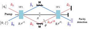
Figure 1: An SU(1,1) interferometer with a two-mode input in which two OPAs take the place of two beam splitters in the traditional Mach-Zehnder interferometer. $g_{1}$ ($g_{2}$) and $\theta_{1}$ ($\theta_{2}$) describe the strength and phase shift in the OPA process $1$ ($2$), respectively. $\hat{a}_{i}$ and $\hat{b}_{i}$ ($i=0,1,2$) mean the annihilation operators of modes $a$ and $b$, respectively. The pump field between the two OPAs has a $\pi$ phase difference compared with the pump field before the first OPA. The output of mode $b_{2}$ is measured by parity detection. M: mirrors, $\phi$: phase shift.

This manuscript is organized as follows: section 2 presents the phase sensitivity in ideal case and the loss effects on the phase sensitivity with the PD which is followed by a comparison among different detections in section 3. Last we conclude with a summary.

2 Phase sensitivity in an SU(1,1) interferometer

2.1 Ideal case

The PD was first proposed by Bollinger et al. [42] to study spectroscopy of trapped ions by counting their number in 1996. Later Gerry [43] introduced the PD into optical interferometers. The PD on an SU(2) interferometer has been proven to be an efficient measurement method for a wide range of input states [44, 45, 46, 47] where the PD works as well, or nearly as well, as state-specific detection schemes [48, 49]. Mathematically, parity here means simply the evenness or oddness of the photon number in an output mode. Its corresponding parity operator is described by $\hat{\Pi}=(-1)^{\hat{N}}$ with $\hat{N}$ being the single-mode photon number operator. In experiments, the PD can be achieved by using homodyne techniques [50] for high power beam, or counting the photon number with a photon-number resolving detector directly for low optical power [51].

In our case, the parity operator of the output mode $b$ is naturally defined as $\hat{\Pi}_{b}\equiv(-1)^{\hat{b}_{2}^{{\dagger}}\hat{b}_{2}}$ where $\hat{b}_{2}$ and $\hat{b}_{2}^{\dagger}$ are annihilation and creation operators of output mode $b$, respectively. According to the linear error propagation formula, the sensitivity of phase estimation with the PD is given by

$$\Delta\phi=\frac{\langle\Delta\hat{\Pi}_{b}\rangle}{\left|\frac{\partial\langle\hat{\Pi}_{b}\rangle}{\partial\phi}\right|},$$ (1)

where $\langle\Delta\hat{\Pi}_{b}\rangle\equiv(\langle\hat{\Pi}_{b}^{2}\rangle-\langle\hat{\Pi}_{b}\rangle^{2})^{1/2}=(1-\langle\hat{\Pi}_{b}\rangle^{2})^{1/2}.$

We consider a coherent and squeezed vacuum state as input here. Transport of input fields through an SU(1,1) interferometer is described in Appendix 6.1. Based on this model, $\langle\hat{\Pi}_{b}\rangle$ is worked out as a series of rather complex and un-illuminating expressions as shown in Appendix 6.2. Then the phase sensitivity in an SU(1,1) interferometer with a coherent and squeezed vacuum input state with the PD is found to be minimal at $\phi=0$ and is given by

$$\Delta\phi=\frac{1}{G_{\mathrm{OPA}}}\frac{1}{\left\{N_{\alpha}[\sinh(2r)\cos(2\theta_{\alpha})+\cosh(2r)]+N_{s}+1\right\}^{1/2}},$$ (2)

where $N_{\alpha}=|\alpha_{0}|^{2}$ is the mean total photon number of input coherent state with $\alpha_{0}=|\alpha_{0}|e^{i\theta_{\alpha}}$ being the amplitude of input coherent state, $N_{s}=\sinh^{2}r$ is the intensity of the squeezed vacuum light with its squeezing parameter $r$, and $G_{\mathrm{OPA}}=\sqrt{N_{\mathrm{OPA}}(N_{\mathrm{OPA}}+2)}=\sinh(2g)$ with $N_{\mathrm{OPA}}=2\sinh^{2}g$ being the spontaneous photon number emitted from the first OPA with the parametric strength of $g$ (we use $g_{1}=g_{2}=g$). When $\theta_{\alpha}=0,$ the optimal phase sensitivity is obtained and is found to be

$$\Delta\phi=\frac{1}{G_{\mathrm{OPA}}}\frac{1}{[(N_{\alpha}e^{2r}+N_{s}+1)]^{1/2}},$$ (3)

where the factor $e^{2r}$ results from the input squeezed vacuum beam. If vacuum input ($N_{s}=0$ and $N_{\alpha}=0$) the phase sensitivity with the PD is then simplified to $\Delta\phi=1/G_{\mathrm{OPA}}$ which is the same as the result of the ID [16]. Thus, the PD has the same optimal scaling of phase sensitivity as the ID with vacuum input.

For the sake of clarity, the corresponding Heisenberg limit (HL) [36] is presented in Appendix 6.3 and is given by

$$\Delta\phi_{\mathrm{HL}}=\frac{1}{N_{\mathrm{Tot}}},$$ (4)

where $N_{\mathrm{Tot}}=(N_{\mathrm{OPA}}+1)N_{\mathrm{in}}+N_{\mathrm{OPA}}$ is the total mean photon number inside the nonlinear interferometer with $N_{\mathrm{in}}=N_{\alpha}+N_{s}$ being the total mean input photon number [37]. Meanwhile, the corresponding shot-noise limit (SNL) is given by $\Delta\phi_{\text{SNL}}=1/\sqrt{N_{\text{Tot}}}$ [36]. According to Ref. [41], it is easy to find another quantum limit, the QCRB of an SU(1,1) interferometer, which is shown in Appendix 6.4.

2.2 Effects of loss

The decoherence process is inevitable by the imperfections in interferometric setups. As discussed in reference [52], there are various kinds of decoherence processes, such as, the effects of phase diffusion, the impact of imperfect visibility and photonic losses. For simplicity, here we only consider the effects of photonic losses. It is well known that loss has a significant effect on the phase sensitivity [53, 54, 55]. In the presence of dissipation, the performance of phase estimation is degraded due to the loss of photons. For this reason, any practical implementation of the measurement scheme must pay special attention to the loss effects carefully.

In this section, we investigate the effects of loss on the phase sensitivity in an SU(1,1) interferometer with the PD. Theoretically, photon loss is typically modeled by a beam splitter that routes photons out of the interferometer as shown in Fig. 2 [33]. $L_{1}$ and $L_{2}$ describe the loss on the up and bottom arms, respectively.

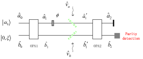
Figure 2: A lossy interferometer model, the losses in the interferometer are modeled by adding fictitious beam splitters. $\hat{v}_{a}$ and $\hat{v}_{b}$ denote the vacuum modes $v_{a}$ and $v_{b}$, respectively.

With this scheme, the pure-state input is now described as a Wigner function for the four modes including two vacuum modes. Due to two external vacuum modes introduced, the initial Wigner function for the four modes is entirely described as

$$W_{\mathrm{in}}(\alpha_{i}^{\prime};\beta_{i}^{\prime};v_{a0};v_{b0})= W_{|\alpha_{0}\rangle}(\alpha_{i},\alpha_{0})W_{|0,\xi\rangle}(\beta_{i},r)$$

$$\times W_{|0\rangle_{a0}}(v_{a0})W_{|0\rangle_{b0}}(v_{b0}),$$ (5)

where $W_{|0\rangle_{a0}}(v_{a0})$ and $W_{|0\rangle_{b0}}(v_{b0})$ are Wigner functions of vacuum in $v_{a}$ and $v_{b}$ modes, respectively, and are given by [38]

$$W_{|0\rangle_{a0}}(v_{a0})=\frac{2}{\pi}e^{-2|v_{a0}|^{2}},$$

$$W_{|0\rangle_{b0}}(v_{b0})=\frac{2}{\pi}e^{-2|v_{b0}|^{2}},$$ (6)

where the complex numbers $v_{a0}$ and $v_{b0}$ are introduced and distributed over the Wigner phase space.

Similar to the ideal case as shown in Appendix 6.1, after passing through the nonlinear interferometer, the corresponding output Wigner function can be then written as

$$W_{\mathrm{out}}(\alpha_{f}^{\prime};\beta_{f}^{\prime};v_{af};v_{bf})= W_{\mathrm{in}}[\alpha_{i}^{\prime}(\alpha_{f}^{\prime};\beta_{f}^{\prime};v_{af};v_{bf});\beta_{i}^{\prime}(\alpha_{f}^{\prime};\beta_{f}^{\prime};v_{af};v_{bf});$$

$$v_{a0}(\alpha_{f}^{\prime};\beta_{f}^{\prime};v_{af};v_{bf});v_{b0}(\alpha_{f}^{\prime};\beta_{f}^{\prime};v_{af};v_{bf})].$$ (7)

Crucially, the four-mode-input-output relation of the SU(1,1) interferometer is given by

$$\left(\begin{array}[]{c}\alpha_{i}\\ \beta_{i}^{\ast}\\ v_{a0}\\ v_{b0}^{\ast}\end{array}\right)=T^{\prime-1}\left(\begin{array}[]{c}\alpha_{f}\\ \beta_{f}^{\ast}\\ v_{af}\\ v_{bf}^{\ast}\end{array}\right),$$ (8)

where the total transformation matrix is found to be

$$T^{\prime}=T_{\mathrm{OPA1}}^{\prime}T_{\phi}^{\prime}T_{\mathrm{loss}}^{\prime}T_{\mathrm{OPA2}}^{\prime},$$

with

$$T_{\mathrm{OPA1}}^{\prime}= \left(\begin{array}[]{cccc}u_{1}&v_{1}&0&0\\ v_{1}^{\ast}&u_{1}&0&0\\ 0&0&1&0\\ 0&0&0&1\end{array}\right),$$ (13)

$$T_{\phi}^{\prime}= \left(\begin{array}[]{cccc}e^{i\phi}&0&0&0\\ 0&1&0&0\\ 0&0&1&0\\ 0&0&0&1\end{array}\right),$$ (18)

$$T_{\mathrm{loss}}^{\prime}= \left(\begin{array}[]{cccc}\sqrt{1-L_{1}}&0&\sqrt{L_{1}}&0\\ 0&\sqrt{1-L_{2}}&0&\sqrt{L_{2}}\\ \sqrt{L_{1}}&0&\sqrt{1-L_{1}}&0\\ 0&\sqrt{L_{2}}&0&\sqrt{1-L_{2}}\end{array}\right),$$ (23)

$$T_{\mathrm{OPA2}}^{\prime}= \left(\begin{array}[]{cccc}u_{2}&v_{2}&0&0\\ v_{2}^{\ast}&u_{2}&0&0\\ 0&0&1&0\\ 0&0&0&1\end{array}\right),$$ (28)

where $u_{k}=\cosh g_{k},v_{k}=e^{i\theta_{k}}\sinh g_{k}$, and $v_{k}^{\ast}$ is the conjugate of $v_{k}$ $(k=1,2)$, $\theta_{1}$ $(\theta_{2})$ and $g_{1}$ $(g_{2})$ are the phase shift and parametric strength in the OPA process 1 (2), respectively. $L_{1}$ and $L_{2}$ denote the photon loss on the modes $a_{1}$ and $b_{1}$ inside the interferometer, respectively.

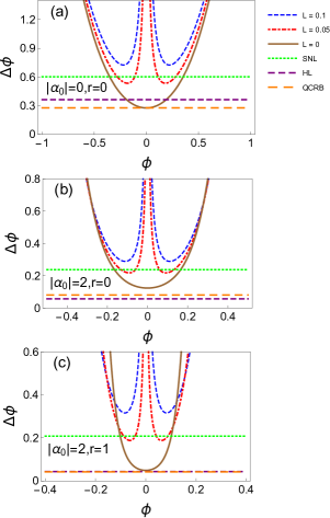
Figure 3: Sensitivity of phase estimation with the PD versus $\phi$ with various inputs of (a) vacuum state ($|\alpha_{0}|=0$ and $r=0$); (b) only one coherent state ($|\alpha_{0}|=2$ and $r=0$); (c) coherent and squeezed vacuum state ($|\alpha_{0}|=2$ and $r=1$), and with different cases of loss: the dashed-blue line is for $L=0.1$, the dash-dotted-red line for $L=0.05$, the solid-brown line for the ideal case, and the dotted-green, dashed-purple, and dashed-orange lines for the SNL, the HL, and the QCRB, respectively. Parameters used are: $L_{1}=L_{2}=L$ and $g=1$.

By combining Eqs. (5), (6), (7), (8), and (49) shown in Appendix 6.1, the signal of the PD on the output of mode $b_{2}$ is given by

$$\langle\hat{\Pi}_{b}^{\mathrm{loss}}\rangle=\frac{\pi}{2}\int W_{\mathrm{out}}(\alpha_{f}^{\prime};0;v_{af};v_{bf})d^{2}\alpha_{f}^{\prime}d^{2}v_{af}d^{2}v_{bf}.$$ (29)

The result of $\langle\hat{\Pi}_{b}^{\mathrm{loss}}\rangle$ is a series of rather large equations, which is reported in Appendix 6.5. Then similar to Eq. (1) the phase sensitivity $\Delta\phi_{\mathrm{L}}$ in the presence of loss is worked out by

$$\Delta\phi_{\mathrm{L}}=\frac{\langle\Delta\hat{\Pi}_{b}^{\mathrm{loss}}\rangle}{\left|\frac{\partial\langle\hat{\Pi}_{b}^{\mathrm{loss}}\rangle}{\partial\phi}\right|},$$ (30)

where the subscript L denotes the loss and the phase sensitivity $\Delta\phi_{\mathrm{L}}$ is also a series of complex expressions and is not reported here.

So far, we have obtained the performance of a nonlinear interferometer via the PD in the presence of loss. Specifically, if vacuum inputs ($\alpha_{0}=0,r=0$), $\Delta\phi_{\mathrm{L}}$ is simplified to

$$\Delta\phi_{\mathrm{L}}= \{1-[(1-L)\sinh^{2}(2g)\cos\phi-(1-L)\cosh^{2}(2g)$$

$$-L\cosh(2g)]^{-2}\}^{1/2}\frac{\csc\phi}{16(1-L)}\{4\coth(2g)[L$$

$$+(1-L)\cosh(2g)]-4(1-L)\sinh(2g)\cos\phi\}^{2},$$ (31)

where we have set $L_{1}=L_{2}=L$. In the absence of loss ($L=0$) and at the optimal phase point ($\phi_{\mathrm{opt}}=0$) the optimal phase sensitivity in Eq. (31) can be reduced to

$$\Delta\phi_{\mathrm{L}}=\frac{1}{G_{\mathrm{OPA}}}=\frac{1}{\sqrt{N_{\text{OPA}}(N_{\text{OPA}}+2)}},$$ (32)

which agrees with the result of ideal case.

It shows the phase sensitivity with the PD as a function of $\phi$ for various cases of loss ($L=0.1,L=0.05$, and $L=0$) under the condition of vacuum state input [one-coherent-state input and coherent $\otimes$ squeezed-vacuum state input] as depicted in Fig. 3(a) [3(b) and 3(c)]. One can easily see that the optimal phase point is at $\phi_{\mathrm{opt}}=0$ in the absence of loss in Figs. 3(a), 3(b), and 3(c). However, considering the effects of loss, $\phi_{\mathrm{opt}}$ becomes apart from $0$. Additionally, the optimal phase point tends to be far away from $0$ with loss increasing. This is due to decorrelation point ($\phi=0$) playing a significant role on precision phase estimation [22]. At nearby the decorrelation point, the detection noise is amplified a little and the optimal phase sensitivity is then obtained. Without loss, $\phi=0$ is the decorrelation point leading that the outputs have the same correlation as inputs. However, $\phi=0$ is not the decorrelation point when considering the effects of photon loss [22] which decreases the precision of phase estimation.

In Fig. 3(a), in the absence of loss, it reaches below the HL ($\Delta\phi_{\text{HL}}=1/N_{\text{OPA}}$) for the optimal sensitivity of phase estimation ($\Delta\phi_{\text{L}}=1/\sqrt{N_{\text{OPA}}(N_{\text{OPA}}+2)}$) with $N_{\text{OPA}}=2\sinh^{2}g$ being the total mean photon number inside the interferometer. However, $N_{\text{OPA}}$ is small because in this scheme the photon number is only dependent on the OPA strength $g$ which is of order of $3$ available currently [56, 18]. Moreover, this sensitivity has been also discussed in Refs. [57, 58]. Although it beats the scaling of $1/N_{\mathrm{Tot}}$ with vacuum state input, one can find that the phase sensitivity approaches but does not reach below the ultimate quantum limit, the QCRB, as depicted in Fig. 3(a). It is worthy noting that it does not surpass the corresponding HL for the optimal sensitivity of phase estimation under the conditions of these two inputs of one-coherent state and coherent $\otimes$ squeezed-vacuum state as depicted in Figs. 3(b) and 3(c), respectively.

Corresponding to Fig. 3(a) [3(b) and 3(c)], the optimal phase sensitivity with the PD as a function of loss is shown in Fig. 4(a) [4(b) and 4(c)]. In Fig. 4(a), one can see that although $\Delta\phi_{\mathrm{L}}$ becomes worse as the loss increases, the optimal sensitivity of phase estimation could still beat the SNL when $L<0.07=L_{\text{cri}}$ where we write this critical loss as $L_{\text{cri}}$ (the subscript cri stands for critical). It is worthy pointing out that $L<0.07$ indicates the lose being less than $7\%$ of photon number on each mode $a_{1}$ and $b_{1}$ between the two OPAs. In the situation of vacuum input considered here, it is $N_{\mathrm{Tot}}\equiv\langle\hat{a}_{1}^{\dagger}\hat{a}_{1}+\hat{b}_{1}^{\dagger}\hat{b}_{1}\rangle=2\sinh^{2}g\approx 2.8$ for the mean total photon number inside the SU(1,1) interferometer. Therefore, it is easily found that $L<0.07$ corresponds the photon number of loss being $0.07N_{\text{Tot}}\approx 0.2$.

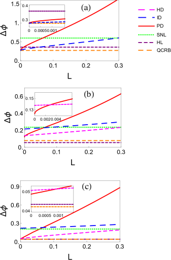
Figure 4: The optimal phase sensitivity with the PD versus the loss $L$ with various inputs of (a) vacuum state ($|\alpha_{0}|=0$ and $r=0$); (b) only one coherent state ($|\alpha_{0}|=2$ and $r=0$); (c) coherent and squeezed vacuum state ($|\alpha_{0}|=2$ and $r=1$). The dashed-magenta, dashed-blue, solid-red, dot-dashed-blue, dashed-purple, and dashed-orange lines correspond to the HD, the ID, the PD, the SNL, the HL, and the QCRB, respectively. It is worthy pointing out that the HD is missing in Fig. 4(a) due to its performance being always bad [62]. Parameter used is: $g=1$.

Moreover, it is worthy pointing out that in Figs. 4(b) and 4(c), the critical losses are $L_{\text{cri}}\approx 0.06$ (for one-coherent-state input with $|\alpha_{0}|=2$ and $g=1$) and $L_{\text{cri}}\approx 0.05$ (for coherent and squeezed-state input with $|\alpha_{0}|=2$, $r=1$, and $g=1$), respectively. One can easily find that they are different for $L_{\text{cri}}$ in Figs. 4(a), 4(b), and 4(c). It is of significance to understand the behaviors of $L_{\text{cri}}$ since $L_{\text{cri}}$ determines whether it achieves a phase sensitivity below the SNL which can not be attainable by classical schemes. Naturally, a new question arises from that how $L_{\text{cri}}$ behaves with different experimental configurations.

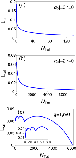
Figure 5: The loss $L_{\text{cri}}$ as a function of $N_{\text{Tot}}$ where only when $L<L_{\text{cri}}$ the $\Delta\phi_{\text{L}}$ reaches below the SNL, with the PD for various cases: (a) vacuum input (varying $g$), (b) one-coherent-state input with a fixed amplitude of $|\alpha_{0}|=2$ (varying $g\in[1,4]$), and (c) one-coherent-state input with a fixed value of $g=1$ (varying $|\alpha_{0}|\in[0,100]$). Note that $N_{\text{Tot}}=(N_{\text{OPA}}+1)N_{\text{in}}+N_{\text{OPA}}$.

To investigate it, we consider three different situations: (1) vacuum state input in Fig. 5(a), (2) one-coherent-state input with a fixed $|\alpha_{0}|=2$ in Fig. 5(b), and (3) one-coherent-state input with a fixed value of $g=1$ in Fig. 5(c)]. It is found that the critical loss $L_{\text{cri}}$ which degrades $\Delta\phi$ to approach the SNL is closely related to the detail configurations, such as, input states and OPA strengths. For instance, considering the vacuum input ($|\alpha|=0$ and $r=0$), let the optimal phase sensitivity $\Delta\phi_{\text{L}}|_{\phi=\phi_{\text{opt}}}=\Delta\phi_{\text{SNL}}$, one can then obtain the relation between the loss $L_{\text{cri}}$ and $g$ which is rather complicated and is not reported here. To make it clear, we plot the $L_{\text{cri}}$ versus $N_{\text{Tot}}$ in Fig. 5(a). It shows that the $L_{\text{cri}}$ decreases with the increase of $g$ which indicates that with $N_{\text{Tot}}$ increasing, it becomes more easily to degrade to the SNL in the presence of loss. Moreover, in Fig. 5(b), the coherent state is fixed by $|\alpha_{0}|=2$ while we adjust $N_{\text{Tot}}$ by varying $g$. It is easily found that $L_{\text{cri}}$ decreases with $N_{\text{Tot}}$ increasing. Furthermore, for comparison, in Fig. 5(c), $g$ is fixed while we vary $|\alpha_{0}|$ to set $N_{\text{Tot}}$. In such a condition, when $N_{\text{Tot}}>4000$, $L_{\text{cri}}$ decreases gradually with the increase of $N_{\text{Tot}}$. However, $L_{\text{cri}}$ fluctuates around $0.06$ when $N_{\text{Tot}}<4000$ which indicates that the phase sensitivity can beat the SNL with a certain loss rate even within a wide range of input intensity.

3 Comparison among different detections in the presence of loss

In a lossy traditional SU(2) interferometer, practical measurements have been compared including the HD, the ID and the PD [59, 60]. Naturally, it is also necessary to compare the performances among the HD, the ID, and the PD in a lossy SU(1,1) interferometer since the SU(1,1) has been realized experimentally [17].

It is worthy noting that the traditional SU(2) interferometer measures the difference in the intensities of the two output modes generally whereas the ID measures the total number of photons at the output in an SU(1,1) interferometer. This is due to for an SU(1,1) interferometer, the intensity difference between the two output modes is a conserved quantity [61] and provides no information about $\phi$ since photons are always created or eliminated in pairs by the parametric processes.

Similar to method in Ref. [36], one can obtain the sensitivity of phase variance with coherent and squeezed vacuum state input in an SU(1,1) interferometer with the ID which is in a rather complicated expression and is shown in Appendix 6.7. Meanwhile, in Ref. [37], it presents the sensitivity of phase estimation with a coherent and squeezed vacuum input state in the presence of loss with the HD,

$$\Delta\phi_{\mathrm{L}}^{\mathrm{H}}=\frac{1}{e^{r}G_{\mathrm{OPA}}\sqrt{N_{\alpha}}}[1+\frac{L}{(1-L)}\frac{e^{2r}N_{\mathrm{Tot}}}{N_{\alpha}+N_{\mathrm{s}}}]^{1/2},$$ (33)

where the superscript H denotes the HD.

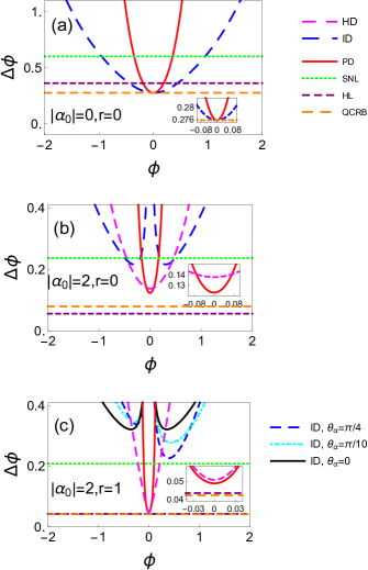
Figure 6: The phase sensitivity with parity detection versus $\phi$ for different detections with various inputs of (a) vacuum state ($|\alpha_{0}|=0$ and $r=0$); (b) only one coherent state ($|\alpha_{0}|=2$ and $r=0$); (c) coherent and squeezed vacuum state ($|\alpha_{0}|=2$ and $r=1$). The dashed-magenta, dashed-blue, solid-red, dot-dashed-blue, dashed-purple, and dashed-orange lines correspond to the HD, the ID, the PD, the SNL, the HL, and the QCRB, respectively. Similar to the Fig. 4(a), the HD is also missing in Fig. 6(a) due to its performance being always bad [62]. Moreover, it is worthy noting that in Fig. 6(c), it plots the phase sensitivities with the ID for different phases of coherent input state. This is owing to that the optimal phase of $\theta_{\alpha}$ is not quite clear with the ID which determines the optimal phase sensitivity to be achieved whereas it is optimal phase $\theta_{\alpha}=0$ for both the HD and the PD. In Fig. 6(c), solid-black, dot-dashed-cyan, and dashed-blue lines denote the ID with $\theta_{\alpha}=0,\pi/10,$ and $\pi/4$, respectively. Parameter used is: $g=1$.

The comparison is performed among the HD, the ID, and the PD for the optimal phase sensitivity as a function of loss $L$ $(L_{1}=L_{2}=L)$ as shown in Fig. 4: (a) vacuum input, (b) one-coherent-state input, and (c) coherent and squeezed-state input, where the dashed-magenta, dashed-blue, solid-red, dotted-green, purple-dashed, and dashed-orange lines stand for the HD, the ID, the PD, the SNL, and the HL, respectively. In Fig. 4(a), we see that with vacuum state input ($|\alpha_{0}|=0$) the ID has a better performance than the PD in the presence of loss. With small loss $L<0.07$ the PD can still surpass the SNL while the ID can beat the SNL even with large loss $L<0.3$. Although the PD has a phase sensitivity as same as the ID in the ideal case as depicted in the zoom figure in Fig. 4(a), the ID is more optimal than the PD in practical experiments in the presence of loss. Moreover, it is worthy pointing out that under the condition of vacuum state input, the HD has a phase sensitivity which is always bad [62]. Therefore, the HD is missing in Fig. 4(a).

In Fig. 4(b), it plots the optimal phase sensitivities for various detections with one-coherent-state input. It is easily found that although without loss the PD has the best phase sensitivity as shown in the corresponding inset figure, the HD becomes the optimal detection scheme with the loss increasing. Moreover, even with large loss $L<0.3$ the HD can still beat the SNL which is a robust scheme to the loss. Furthermore, it is worthy noting that with one-coherent-state input the ID has a optimal phase sensitivity which is around the SNL and is worst than the ones of the HD and ID. To explain this, we plot the phase sensitivities of the HD, the ID, and the PD versus $\phi$ in the absence of loss as shown in Fig. 6(b). One can easily find that the ID has a phase sensitivity which diverges at $\phi=0$ whereas $\phi=0$ is the optimal phase point for both the HD and the PD. Therefore, the ID has a worse optimal phase sensitivity which is not suitable for the case of one-coherent-state input in a nonlinear interferometer. However, the ID has a phase sensitivity which degrades a little with the increase of loss as depicted in Fig. 4(b). Therefore, even with a worse optimal phase sensitivity, the ID is robust to the loss.

Fig. 4(c) presents the optimal phase sensitivities of the HD, the ID, and the PD versus loss $L$ with the input of coherent and squeezed state. In the absence of loss, the optimal phase sensitivities of HD and PD are close to the HL whereas it is around the SNL for the optimal phase sensitivity with the ID. Similar to the case of one-coherent-state input, the PD has the best optimal phase sensitivity without loss with coherent and squeezed-state input as shown in the zoom figure in Fig. 4(c). However, it degrades sharply for the optimal phase sensitivity of the PD with the loss increasing while the ones of the ID and HD degrade a little.

Corresponding to Fig. 4(c), it plots the phase sensitivities in the absence of loss as a function of $\phi$ with coherent and squeezed-state input for various detection schemes in Fig. 6(c). It is worthy pointing out that it diverges at $\phi=0$ for the phase sensitivity of the ID which is similar to the case of one-coherent-state input. Moreover, it is found that the phase sensitivity is related the phase of coherent input state $\theta_{\alpha}$ where $\theta_{s}$ has been set to zero for the phase of the squeezed input state. Therefore, it also plots the phase sensitivities for various $\theta_{\alpha}=0,\pi/10,$ and $\pi/4$ in Fig. 6(c). It is worthy noting that when $\theta_{\alpha}=0$, it is symmetrical for the phase sensitivity with the ID along with the line of $\phi=0$ whereas it is not symmetrical any more when $\theta_{\alpha}=\pi/10$ and $\pi/4$. However, if $\theta_{\alpha}=\pi/4$, it has a better optimal phase sensitivity than the cases of $\theta_{\alpha}=0$ and $\pi/10$.

Although the ID achieves its optimal phase sensitivity as well as the scaling of phase sensitivity as shown in Fig. 4(c), it is close to the SNL which looks like not consistent with the conclusion of beating the SNL as reported in previous works [63, 36]. In fact, the results do not contradict each other. In Refs. [63, 36], they presented that the ID is proven to be an efficient detection scheme in which the input is in a two-coherent state whereas the input is in a coherent and squeezed state in our scheme. Therefore, the input considered here is different from the previous works which leads to a medium performance of phase sensitivity with the ID.

To verify this, it is investigated for the case of two-equal-coherent state as input. Similarly, the comparison is performed among these three detections in an SU(1,1) interferometer in the following content. According to Ref. [36], it can be found that the optimal sensitivity of phase estimation with the ID with considering loss with two-equal-coherent-state input $|i\alpha_{0}/\sqrt{2}\rangle\otimes|\alpha_{0}/\sqrt{2}\rangle$ is given by

$$\Delta\phi_{\text{L,twocoh}}^{\text{I}}= \{\frac{1}{4|\alpha_{0}|^{2}\sinh^{2}g\cosh^{2}g}[1+\frac{L}{1-L}(1+2\sinh^{2}g)]$$

$$+\frac{L}{(1-L)^{2}}\frac{1+L(\sinh^{2}g+\cosh^{2}g)}{4|\alpha_{0}|^{2}\cosh^{2}g}\}^{1/2},$$ (34)

where for convenience, we have used $g$, $1-L$, $i\alpha_{0}/\sqrt{2}$ and $\alpha_{0}/\sqrt{2}$ to replace the $s$, $\eta_{1}$, $\alpha$ and $\beta$ in the expression of Eq. (23) in Ref. [36], respectively. Similar to the method as discussed in Ref. [37], one can obtain the optimal phase sensitivity with the HD with two-equal-coherent-state input as

$$\Delta\phi_{\text{L,twocoh}}^{\text{H}}= \sqrt{\frac{L\cosh(2g)+1-L}{1-L}}\frac{1}{\sqrt{2}|\alpha_{0}|\cosh^{2}g(\tanh g+1)}$$

$$= \sqrt{\frac{L\cosh(2g)+1-L}{1-L}}\times$$

$$\frac{\sqrt{2}}{|\alpha_{0}|(\sqrt{N_{\text{OPA}}(N_{\text{OPA}}+2)}+N_{\text{OPA}}+2)},$$ (35)

where we have used $N_{\text{OPA}}\equiv 2\sinh^{2}g$ which means the spontaneous photon number generated by the fisrt OPA when the input state is in a vacuum state.

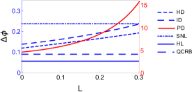
Figure 7: The optimal phase sensitivity $\Delta\phi$ of the SU(1,1) interferometer as a function of loss $L$ for different detection schemes (HD, ID, and PD) with two-equal-coherent-state input $|i\alpha_{0}/\sqrt{2}\rangle\otimes|\alpha_{0}/\sqrt{2}\rangle$. The short-dashed-blue, long-dashed-blue, solid-red, dot-dashed-blue, and solid-blue lines correspond to the HD, the ID, the PD, the SNL, and the HL, respectively. It is worthy pointing out that the four blue lines are related to the blue scaling on the left side of frame while the red line corresponds to the red scaling on the right side one. Parameters used are: $|\alpha_{0}|=2$ and $g=1$.

In Fig. 7, we plot the optimal sensitivities of phase estimation as a function of loss with two-equal-coherent-state input $|i\alpha_{0}/\sqrt{2}\rangle\otimes|\alpha_{0}/\sqrt{2}\rangle$ for various detection schemes. The short-dashed-blue, long-dashed-blue, solid-red, dot-dashed-blue, solid-blue, and dashed-orange lines correspond to the HD, the ID, the PD, the SNL, the HL, and the QCRB, respectively. It is worthy pointing out that the five blue lines are related to the blue scaling on the left side of frame while the red line corresponds to the red scaling on the right side one. One can easily find that the HD has the best optimal sensitivity of phase estimation among those three detection schemes while the PD has a phase sensitivity which is worst under the condition of two-equal-coherent-state input. Moreover, it is worthy noting that although the ID has a medium performance, it still surpasses the SNL even with loss of $L=30\%$ which is different from the cases of one-coherent-state and coherent $\otimes$ squeezed-state inputs. Furthermore, it is easily to find that both the HD and the ID are robust to the loss where the optimal phase sensitivities degrade a little with the increase of the loss as depicted in Fig. 7.

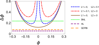
Figure 8: The phase sensitivity $\Delta\phi$ of the SU(1,1) interferometer as a function of $\phi$ with the loss on the phase sensing arm (dot-dashed-red line) and the free arm (dashed-blue line), respectively. The solid-brown line presents the ideal case. The dashed-green, dashed-purple, and dashed-orange lines denote the SNL, the HL, and the QCRB, respectively. Parameters used are: $|\alpha_{0}|=2$, $r=0$, and $g=1$.

It has been studied for the case of the same value of loss ($L_{1}=L_{2}$) on the two arms between the two OPAs in the previous section. Here we will discuss the phase sensitivity in the presence of different values of loss, $L_{1}\neq L_{2}$, where the result is shown in Appendix 6.8. In Fig. 8, we plot the sensitivities as a function of $\phi$ in the presence of loss only on the phase sensing arm (dot-dashed-red line: $L_{1}=0.1,L_{2}=0$) or the free arm (dashed-blue line: $L_{1}=0,L_{2}=0.1$), respectively. It is shown that the sensitivity reduction by the loss on the phase sensing arm is larger. This is due to the fact that the loss on the phase sensing arm degrades the phase information directly which has a significant impact on the sensitivity of phase estimation. Therefore, we should pay much more attention on the loss on the arm experiencing phase shift in experiments.

4 Conclusion

In conclusion we study the effects of loss on the phase sensitivity in an SU(1,1) interferometer with the PD. The effects of loss have a significant role on the sensitivity of phase estimation with the PD while the PD still serves as an optimal strategy when considering the phase fluctuations [40]. This is due to photon loss distorting the parity of photon number for the PD to estimate the phase variance. In the presence of small loss, the PD still surpasses the SNL. Moreover, we also compare the performance among the HD, the ID, and the PD in a lossy nonlinear interferometer with various state inputs. It is found that when the input is in a vacuum state, the ID is the optimal detection in the presence of loss while the HD is the optimal measurement when the input is in a one-coherent state, coherent $\otimes$ squeezed state, or two-equal-coherent state in the presence of loss.

5 Acknowledge

Dong Li is supported by the Science Challenge Project under Grant No. TZ2018003-3. Chun-Hua Yuan is supported by the National Natural Science Foundation of China under Grant No. 11474095 and the Fundamental Research Funds for the Central Universities. Yao Yao is supported by the National Natural Science Foundation of China under Grant No. 11605166. Weiping Zhang acknowledges support from National Key Research and Development Program of China under Grant No. 2016YFA0302001, the National Natural Science Foundation of China (Grants No. 11654005, No. 11234003, and No. 11129402), and the Science and Technology Commission of Shanghai Municipality (Grant No. 16DZ2260200).

6 Appendix

6.1 Model

We review the model as discussed in Ref. [41]. The schematic of an SU(1,1) interferometer is shown in Fig. 1 where the OPAs take the place of the 50-50 beam splitters in a traditional MZI. Here a coherent light mixed with a squeezed vacuum state is considered as the input. The annihilation (creation) operators of the two modes are denoted by $\hat{a}$ $(\hat{a}^{{\dagger}})$ and $\hat{b}$ $(\hat{b}^{{\dagger}})$. The propagation of the beams through the SU(1,1) interferometer is described as follow: after the first OPA, one output is retained as a reference, while the other one experiences a phase shift; after the beams recombine in the second OPA with the reference field, the output lights are dependent on the phase difference $\phi$ between the two modes.

For simplicity, we consider the phase space to describe the propagation. The Wigner function of the input state, a product state $|\alpha_{0}\rangle\otimes|0,\xi=re^{i\theta_{s}}\rangle$, with coherent light amplitude $\alpha_{0}=|\alpha_{0}|e^{i\theta_{\alpha}}$, is written as

$$W_{\mathrm{in}}(\alpha_{i},\alpha_{0};\beta_{i},r)=W_{|\alpha_{0}\rangle}(\alpha_{i},\alpha_{0})W_{|0,\xi\rangle}(\beta_{i},r),$$ (36)

where the Wigner functions of coherent and squeezed vacuum states are given by [38]

$$W_{|\alpha_{0}\rangle}(\alpha_{i},\alpha_{0}) =\frac{2}{\pi}e^{-2|\alpha_{i}-\alpha_{0}|^{2}},$$ (37)

$$W_{|0,\xi\rangle}(\beta_{i},r) =\frac{2}{\pi}e^{-2|\beta_{i}|^{2}\cosh 2r+(\beta_{i}^{2}+\beta_{i}^{\ast 2})\sinh 2r},$$ (38)

respectively, with $\theta_{s}=0$ by appropriately fixing the irrelevant absolute phase $\theta_{\alpha}$, and $\beta_{i}^{\ast}$ is the conjugate of $\beta_{i}$.

After propagation through the SU(1,1) interferometer the output Wigner function is found to be

$$W_{\mathrm{out}}(\alpha_{f},\beta_{f})=W_{\mathrm{in}}[\alpha_{i}(\alpha_{f},\beta_{f}),\beta_{i}(\alpha_{f},\beta_{f})],$$ (39)

where $\alpha_{i},\beta_{i},\alpha_{f}$ and $\beta_{f}$ are the complex amplitudes of the beams in the mode $\hat{a}_{0},\hat{b}_{0},\hat{a}_{2}$, and $\hat{b}_{2}$, respectively. Generally, propagations through the first OPA, phase shift, and second OPA are given by

$$T_{\mathrm{OPA1}}=\left(\begin{array}[]{cc}u_{1}&v_{1}\\ v_{1}^{\ast}&u_{1}\end{array}\right),\quad\quad T_{\phi}=\left(\begin{array}[]{cc}e^{i\phi}&0\\ 0&1\end{array}\right),\quad\quad T_{\mathrm{OPA2}}=\left(\begin{array}[]{cc}u_{2}&v_{2}\\ v_{2}^{\ast}&u_{2}\end{array}\right),$$ (46)

with $u_{k}=\cosh g_{k},v_{k}=e^{i\theta_{k}}\sinh g_{k}$, and $v_{k}^{\ast}$ being the conjugate of $v_{k}$ $(k=1,2)$, where $\theta_{1}$ $(\theta_{2})$ and $g_{1}$ $(g_{2})$ are the phase shift and parametric strength in the OPA process 1 (2), respectively, see, for example Ref. [64]. Therefore, the nonlinear interferometer is described by $T=T_{\mathrm{OPA2}}T_{\phi}T_{\mathrm{OPA1}}$. Thus, the relation between variables is given by

$$\left(\begin{array}[]{c}\alpha_{i}\\ \beta_{i}^{\ast}\end{array}\right)=T^{-1}\left(\begin{array}[]{c}\alpha_{f}\\ \beta_{f}^{\ast}\end{array}\right).$$ (47)

More specifically, we assume that the first OPA and the second one have a $\pi$ phase difference (particularly $\theta_{1}=0$ and $\theta_{2}=\pi$) and same parametric strength ($g_{1}=g_{2}=g$). In such a case, the second OPA will undo what the first one does (namely $\hat{a}_{2}=\hat{a}_{0}$ and $\hat{b}_{2}=\hat{b}_{0}$) if phase shift $\phi=0$, which we call the balanced situation.

In the case of the balanced situation, the relation between the input and output variables is found to be

$$T^{-1}=\left(\begin{array}[]{cc}G&R\\ -R&H\end{array}\right),$$

where $G=A-iB\cosh(2g),H=A+iB\cosh(2g)$ and $R=-iB\sinh(2g)$ with $A=\cos(\phi/2)e^{-i\phi/2}$ and $B=\sin(\phi/2)e^{-i\phi/2}$. The output Wigner function of the SU(1,1) interferometer is then obtained,

$$W_{\mathrm{out}}(\alpha_{f},\beta_{f})= \frac{4}{\pi^{2}}e^{-2|G\alpha_{f}+R\beta_{f}^{\ast}-\alpha_{0}|^{2}-2|-R\alpha_{f}+H\beta_{f}^{\ast}|^{2}\cosh(2r)}e^{2\mathrm{Re}[(-R\alpha_{f}+H\beta_{f}^{\ast})^{2}]\sinh(2r)}.$$ (48)

Alternatively, according to Ref. [65], the parity signal is given by

$$\langle\hat{\Pi}_{b}\rangle=\frac{\pi}{2}\int W_{\mathrm{out}}(\alpha_{f},0)d^{2}\alpha_{f},$$ (49)

6.2 Parity detection signal in ideal case

According to Eqs. (48) and (49), the detection signal $\langle\hat{\Pi}_{b}\rangle$ is worked out as

$$\langle\hat{\Pi}_{b}\rangle=\frac{1}{\sqrt{x_{1}}}e^{-x_{2}/x_{3}},$$ (50)

where

$$x_{1}= e^{-2r}(e^{2r}+1)^{2}[8\sinh^{4}(2g)(\cos(2\phi)-\cos\phi)+4\cosh(4g)+3\cosh(8g)-7]+64,$$

$$x_{2}= 4|\alpha|^{2}\sinh^{2}(2g)\{8\cosh(4g)\cos(2\theta)\sin^{4}(\phi/2)-8\cosh(2g)\sin(2\theta)\sin\phi(\cos\phi-1)$$

$$+8e^{4r}[\cos\theta\sin\phi-2\cosh(2g)\sin\theta\sin^{2}(\phi/2)]^{2}+32e^{2r}\sinh^{2}(2g)\sin^{4}(\phi/2)$$

$$+8\cosh(4g)\sin^{4}(\phi/2)-8\cos^{2}\theta\cos\phi+[3\cos(2\theta)-1]\cos(2\phi)+\cos(2\theta)+5\},$$

$$x_{3}= (e^{2r}+1)^{2}[8\cosh(8g)\sin^{4}(\phi/2)+8\cosh(4g)\sin^{2}\phi+4\cos\phi+3\cos(2\phi)-7]+64e^{2r}.$$ (51)

Assuming that $\phi=0,$ the signal is then simplified to

$$\langle\hat{\Pi}_{b}\rangle|_{\phi=0}=1.$$ (52)

This is due to the second OPA would undo what the first one did if $\phi=0$. Meanwhile the output field is the same as the input. Thus the output in mode $b$ is the one-mode squeezed vacuum. The measurement signal is one with the one-mode squeezed vacuum input causing only even number distribution in the Fock basis with $|0,\xi=re^{i\phi_{s}}\rangle=\sqrt{1/\cosh r}\sum_{n=0}^{\infty}(\sqrt{(2n)!}/n)(1/2)^{n}[\exp(i\phi_{s})\tanh r]^{n}|2n\rangle$ [66].

6.3 Heisenberg limit and shot-noise limit

Here, we focus on the HL in an SU(1,1) interferometer. According to Ref. [36], the HL corresponds to the total number of photons $N_{\mathrm{Tot}}(\equiv\langle\hat{a}_{1}^{\dagger}\hat{a}_{1}+\hat{b}_{1}^{\dagger}\hat{b}_{1}\rangle)$ inside the SU(1,1) interferometer not the input photon number as the traditional MZI. This is due to amplification of the phase sensing photon number by the first OPA. Then the corresponding HL is given by

$$\Delta\phi_{\mathrm{HL}}=\frac{1}{N_{\mathrm{Tot}}},$$ (53)

where the subscript HL represents Heisenberg limit. According to Ref. [37] the total inside photon number is given by

$$N_{\mathrm{Tot}}=(N_{\mathrm{OPA}}+1)N_{\mathrm{in}}+N_{\mathrm{OPA}},$$ (54)

where $N_{\mathrm{in}}=N_{\alpha}+N_{s}$. The first term of equation (54) on the right-hand side, $(N_{\mathrm{OPA}}+1)N_{\mathrm{in}}$, results from the amplification process of the input photon number and the second one is related to the spontaneous process. Thus the total inside photon number $N_{\mathrm{Tot}}$ corresponds to not only the OPA strength but also the input photon number. Then the corresponding SNL is written as

$$\Delta\phi_{\mathrm{SNL}}=\frac{1}{\sqrt{N_{\mathrm{Tot}}}},$$ (55)

where the subscript SNL denotes the shot-noise limit.

6.4 Quantum Cramér-Rao bound

According to Ref. [41], one can easily find the QCRB of an SU(1,1) interferometer with different input states which are shown in the table as follows.

Table 1: The quantum Cramér-Rao bound (QCRB) of an SU(1,1) interferometer with different input states.

Input states	QCRB
$|0\rangle\otimes|0\rangle$	$1/\mathcal{K}^{1/2}$
$|\alpha_{0}\rangle\otimes|0\rangle$	$1/[\mathcal{K}(2N_{\alpha}+1)+2N_{\alpha}(N_{\text{OPA}}+2)]^{1/2}$
$|\frac{i\alpha_{0}}{\sqrt{2}}\rangle\otimes|\frac{\alpha_{0}}{\sqrt{2}}\rangle$	$1/\{2N_{\alpha}[(N_{\text{OPA}}+1)\sqrt{\mathcal{K}}+\mathcal{K}+1]+\mathcal{K}\}^{1/2}$
$|\alpha_{0}\rangle\otimes|0,\xi\rangle$	$1/[2N_{\alpha}(N_{\text{OPA}}+2)+N_{\text{OPA}}^{2}\sinh^{2}(2r)/2+\mathcal{K}(2N_{\alpha}\cosh re^{r}+\cosh^{2}r)]^{1/2}$

where $\mathcal{K}=N_{\text{OPA}}(N_{\text{OPA}}+2)$. Row 1: vacuum input state; Row 2: one-coherent input state; Row 3: two-coherent input state; Row 4: coherent mixed with squeezed-vacuum input state.

6.5 Parity detection signal in the presence of loss

According to Eqs. (7), (8), and (29), the parity signal in the presence of loss is given by

$$\langle\hat{\Pi}_{b}^{\mathrm{loss}}\rangle=\frac{8}{\sqrt{y_{1}}}e^{-\frac{y_{2}}{y_{3}}},$$ (56)

where

$$y_{1}= e^{-2r}(-4\cosh(4g)(-2(5L^{2}-2L+1)e^{2r}+(L-1)^{2}(e^{2r}+1)^{2}\cos(2\phi)+(L-1)^{2}(-e^{4r})-(L-1)^{2})+16(L-1)^{2}e^{2r}\cosh(6g)\cos\phi$$

$$+8(L-1)^{2}e^{4r}\cosh(6g)\cos\phi-8(L-1)^{2}e^{2r}\cosh(8g)\cos\phi-4(L-1)^{2}e^{4r}\cosh(8g)\cos\phi+2(L-1)^{2}e^{2r}\cosh(8g)\cos(2\phi)$$

$$+(L-1)^{2}e^{4r}\cosh(8g)\cos(2\phi)+16(L-1)e^{2r}\cosh(6g)\cos\phi+8(L-1)e^{4r}\cosh(6g)\cos\phi+8(1-L)L\cosh(2g)((e^{2r}+1)^{2}\cos\phi$$

$$-2e^{2r}+7e^{4r}+7)-16(L-1)^{2}e^{2r}\cosh(6g)-8(L-1)^{2}e^{4r}\cosh(6g)+6(L-1)^{2}e^{2r}\cosh(8g)+3(L-1)^{2}e^{4r}\cosh(8g)$$

$$-16(L-1)e^{2r}\cosh(6g)-8(L-1)e^{4r}\cosh(6g)+8(L-1)^{2}\cosh(6g)\cos\phi-4(L-1)^{2}\cosh(8g)\cos\phi+(L-1)^{2}\cosh(8g)\cos(2\phi)$$

$$+8(L-1)\cosh(6g)\cos\phi-8(L-1)^{2}\cosh(6g)+3(L-1)^{2}\cosh(8g)-8(L-1)\cosh(6g)+8(L-1)^{2}e^{2r}\cos\phi+4(L-1)^{2}e^{4r}\cos\phi$$

$$+6(L-1)^{2}e^{2r}\cos(2\phi)+3(L-1)^{2}e^{4r}\cos(2\phi)+82(L-1)^{2}e^{2r}-7(L-1)^{2}e^{4r}+64(L-1)e^{2r}+4(L-1)^{2}\cos\phi+3(L-1)^{2}\cos(2\phi)$$

$$-7(L-1)^{2}+32e^{2r}),$$

$$y_{2}= 16|\alpha_{0}|^{2}(1-L)\sinh^{2}(2g)\sin^{2}(\frac{\phi}{2})(2(L-1)(e^{2r}(\cosh(4g)-1)\times(\cos\phi-1)+(\cosh(4g)+1)(\cos\phi-1)$$

$$-2e^{4r}(\cos\phi+1))+8Le^{2r}\cosh(2g)),$$

$$y_{3}= -8(L-1)^{2}(e^{2r}+1)^{2}\sinh^{2}(4g)\cos\phi+2e^{2r}(8(L-2)L\sinh^{4}(2g)\cos(2\phi)+4(L(5L-2)+1)\cosh(4g)-8(L-1)L\cosh(6g)$$

$$+3(L-1)^{2}\cosh(8g)+8\sinh^{4}(2g)\cos(2\phi)+L(41L-50)+25)+(L-1)e^{4r}((L-1)(8\sinh^{4}(2g)\cos(2\phi)+3\cosh(8g)-7)$$

$$+4(L-1)\cosh(4g)-8L\cosh(6g))+8(L-1)L\cosh(2g)\times(4(e^{2r}+1)^{2}\sinh^{2}(2g)\cos\phi+2e^{2r}-7e^{4r}-7)$$

$$+(L-1)((L-1)(8\sinh^{4}(2g)\cos(2\phi)+3\cosh(8g)-7)+4(L-1)\cosh(4g)-8L\cosh(6g)).$$ (57)

6.6 Phase sensitivity with the PD with one-coherent-state input with the same loss on the two arms

If one-coherent state is injected, according to Eqs. (29) and (30), the phase sensitivity in the presence of loss is worked out as

$$\Delta\phi_{\mathrm{L}}=\sqrt{\frac{z_{1}}{z_{2}}},$$ (58)

where

$$z_{1}= 1-\frac{4\exp(\frac{8|\alpha_{0}|^{2}(L-1)\sinh^{2}(2g)\sin^{2}(\frac{\phi}{2})}{2L\cosh(2g)-(L-1)(-2\sinh^{2}(2g)\cos\phi+\cosh(4g)+1)})}{((L-1)(-2\sinh^{2}(2g)\cos\phi+\cosh(4g)+1)-2L\cosh(2g))^{2}},$$

$$z_{2}= 256\frac{k_{1}}{k_{2}}e^{k_{3}},$$ (59)

with

$$k_{1}= (1-L)^{2}\sinh^{4}(2g)\sin^{2}\phi(-4(|\alpha_{0}|^{2}+1)L\cosh(2g)+2(1-L)\cosh(4g)\cos\phi-(2-2L)\cosh(4g)$$

$$-4|\alpha_{0}|^{2}(1-L)-2(1-L)\cos\phi-3(1-L)-L+1)^{2},$$

$$k_{2}= (4(1-L)\sinh^{2}(2g)\cos(\phi)-4L\cosh(2g)-(2-2L)\cosh(4g)-3(1-L)-L+1)^{6},$$

$$k_{3}= [4|\alpha_{0}|^{2}\sinh^{2}(2g)(-2(1-L)\cos\phi-2L+2)]/[4(1-L)\sinh^{2}(2g)\cos\phi-4L\cosh(2g)-(2-2L)\cosh(4g)$$

$$-3(1-L)-L+1].$$ (60)

6.7 Phase sensitivity via the ID in the presence of loss

If one-coherent state is injected with the loss of $L_{1}=L_{2}=L$, the phase sensitivity with the ID is found to be

$$\Delta\phi_{\text{L}}^{\text{I}}= \{\text{csch}^{4}(2g)[\csc^{2}(\frac{\phi}{2})(2(|\alpha_{0}|^{2}+1)L(1-L)\cosh(2g)+2|\alpha_{0}|^{2}(1-L)^{2}+L^{2}\cosh(4g)-(2-L)L)$$ (61)

$$+\sec^{2}(\frac{\phi}{2})((2|\alpha_{0}|^{2}+1)(1-L)^{2}\cosh(8g)+2(|\alpha_{0}|^{2}+1)L(1-L)\cosh(6g)+L^{2}\cosh(4g)-1)]$$

$$-8(2|\alpha_{0}|^{2}+1)(1-L)^{2}\}^{1/2}(|\alpha_{0}|^{2}+1)^{-1}(1-L)^{-1}8^{-1/2}.$$

If vacuum state input ($|\alpha_{0}|=0$) with the loss of $L_{1}=L_{2}=L$, the phase sensitivity with the ID is found to be

$$\Delta\phi_{\text{L}}^{\text{I}}= \{\text{csch}^{4}(2g)[\csc^{2}(\frac{\phi}{2})(L^{2}\cosh(4g)+2(1-L)L\cosh(2g)-(2-L)L)+\sec^{2}(\frac{\phi}{2})(L^{2}\cosh(4g)$$ (62)

$$+(1-L)^{2}\cosh(8g)+2L(1-L)\cosh(6g)-1)]+8(1-L)^{2}\}^{1/2}(1-L)^{-1}8^{-1/2}.$$

6.8 Phase sensitivity with the PD with one-coherent-state input with different losses on the two arms

If one coherent state input is considered as input, with different losses, $L_{1}\neq L_{2}$, the phase sensitivity is found to be

$$\Delta\phi_{\mathrm{L}}=\sqrt{\frac{f_{1}}{f_{2}}},$$ (63)

where

$$f_{1}=1-\frac{4}{c_{2}}e^{c_{1}},$$

$$f_{2}=256\frac{d_{1}}{d_{2}}e^{d_{3}},$$ (64)

with

$$c_{1}= -[2|\alpha_{0}|^{2}\sinh^{2}(2g)(2\sqrt{1-L_{1}}\sqrt{1-L_{2}}\cos\phi+L_{1}+L_{2}-2)]/[2\sqrt{1-L_{1}}\sqrt{1-L_{2}}\sinh^{2}(2g)\cos\phi+4L_{1}\sinh^{4}(g)$$

$$+L_{2}\sinh^{2}(2g)-\cosh(4g)-1],$$

$$c_{2}= (-2\sqrt{1-L_{1}}\sqrt{1-L_{2}}\sinh^{2}(2g)\cos(\phi)-4L_{1}\sinh^{4}(g)-L_{2}\sinh^{2}(2g)+\cosh(4g)+1)^{2},$$

$$d_{1}= (1-L_{1})(1-L_{2})\sinh^{4}(2g)\sin^{2}\phi(-4(|\alpha_{0}|^{2}+1)L_{1}\cosh(2g)+2\sqrt{1-L_{1}}\sqrt{1-L_{2}}\cosh(4g)\cos\phi-(-L_{1}-L_{2}+2)\cosh(4g)$$

$$-4|\alpha_{0}|^{2}(1-L_{1})-2\sqrt{1-L_{1}}\sqrt{1-L_{2}}\cos\phi-3(1-L_{1})-L_{2}+1)^{2},$$

$$d_{2}= (4\sqrt{1-L_{1}}\sqrt{1-L_{2}}\sinh^{2}(2g)\cos\phi-4L_{1}\cosh(2g)-(-L_{1}-L_{2}+2)\cosh(4g)-3(1-L_{1})-L_{2}+1)^{6},$$

$$d_{3}= [4|\alpha_{0}|^{2}\sinh^{2}(2g)(-2\sqrt{1-L_{1}}\sqrt{1-L_{2}}\cos\phi-L_{1}-L_{2}+2)]/[4\sqrt{1-L_{1}}\sqrt{1-L_{2}}\sinh^{2}(2g)\cos\phi$$

$$-4L_{1}\cosh(2g)-(2-L_{1}-L_{2})\cosh(4g)-3(1-L_{1})-L_{2}+1].$$ (65)

References

- [1] C. W. Helstrom, Quantum detection and estimation theory (Academic press, 1976).
- [2] A. S. Holevo, Probabilistic and statistical aspects of quantum theory (Springer Science, 2011).
- [3] C. M. Caves, “Quantum-mechanical noise in an interferometer,” Phys. Rev. D 23, 1693 (1981).
- [4] M. Xiao, L.-A. Wu, and H. J. Kimble, “Precision measurement beyond the shot-noise limit,” Phys. Rev. Lett. 59, 278 (1987).
- [5] S. L. Braunstein and C. M. Caves, “Statistical distance and the geometry of quantum states,” Phys. Rev. Lett. 72, 3439 (1994).
- [6] R. Demkowicz-Dobrzański, J. Kołodyński, and M. Guţă, “The elusive Heisenberg limit in quantum-enhanced metrology,” Nat. Commun. 3, 1063 (2012).
- [7] H. Lee, P. Kok, and J. P. Dowling, “A quantum rosetta stone for interferometry,” Journal of Modern Optics 49, 2325 (2002).
- [8] V. Giovannetti, S. Lloyd, and L. Maccone, “Quantum-enhanced measurements: beating the standard quantum limit,” Science 306, 1330 (2004).
- [9] Y. Gao, P. M. Anisimov, C. F. Wildfeuer, J. Luine, H. Lee, and J. P. Dowling, “Super-resolution at the shot-noise limit with coherent states and photon-number-resolving detectors,” J. Opt. Soc. Am. B 27, A170–A174 (2010).
- [10] J. P. Dowling, “Quantum optical metrology–the lowdown on high-N00N states,” Contemporary physics 49, 125 (2008).
- [11] K. Berrada, “Quantum metrology with classical light states in non-Markovian lossy channels,” J. Opt. Soc. Am. B 34, 1912–1917 (2017).
- [12] Stuart S. Szigeti, Robert J. Lewis-Swan, and Simon A. Haine, “Pumped-Up SU(1,1) Interferometry,” Phys. Rev. Lett. 118, 150401 (2017).
- [13] F. Anders, L. Pezzè, A. Smerzi, and C Klempt, “Phase magnification by two-axis counter-twisting for detection noise robust interferometry,” arXiv:1711.02658.
- [14] B. P. Abbott, R. Abbott, T. D. Abbott, M. R. Abernathy, F. Acernese, K. Ackley, C. Adams, T. Adams, P. Addesso, R. X. Adhikari et al., “GW150914: The advanced LIGO detectors in the era of first discoveries,” Phys. Rev. Lett. 116, 131103 (2016).
- [15] K. P. Seshadreesan, S. Kim, J. P. Dowling, and H. Lee, “Phase estimation at the quantum Cramér-Rao bound via parity detection,” Phys. Rev. A 87, 043833 (2013).
- [16] B. Yurke, S. L. McCall, and J. R. Klauder, “SU(2) and SU(1,1) interferometers,” Phys. Rev. A 33, 4033 (1986).
- [17] J. Jing, C. Liu, Z. Zhou, Z. Y. Ou, and W. Zhang, “Realization of a nonlinear interferometer with parametric amplifiers,” Appl. Phys. Lett. 99, 011110 (2011).
- [18] F. Hudelist, J. Kong, C. Liu, J. Jing, Z. Y. Ou, and W. Zhang, “Quantum metrology with parametric amplifier-based photon correlation interferometers,” Nat. Commun. 5, 3049 (2014).
- [19] B. E. Anderson, P. Gupta, B. L. Schmittberger, T. Horrom, C. Hermann-Avigliano, K. M. Jones, and P. D. Lett, “Phase sensing beyond the standard quantum limit with a variation on the SU(1,1) interferometer,” Optica 4, 752–756 (2017).
- [20] B. Chen, C. Qiu, S. Chen, J. Guo, L. Q. Chen, Z. Y. Ou, and W. Zhang, “Atom-light hybrid interferometer,” Phys. Rev. Lett. 115, 043602 (2015).
- [21] H. Ma, D. Li, C.-H. Yuan, L. Chen, Z. Ou, and W. Zhang, “SU(1, 1)-type light-atom-correlated interferometer,” Phys. Rev. A 92, 023847 (2015).
- [22] Z. D. Chen, C. H. Yuan, H. M. Ma, D. Li, L. Q. Chen, Z. Y. Ou, and W. Zhang, “Effects of losses in the atom-light hybrid SU(1,1) interferometer,” Optics Express 24, 17766 (2016).
- [23] C. Gross, T. Zibold, E. Nicklas, J. Esteve, and M. K. Oberthaler, “Nonlinear atom interferometer surpasses classical precision limit,” Nature 464, 1165 (2010).
- [24] J. Peise, B. Lücke, L. Pezzè, F. Deuretzbacher, W. Ertmer, J. Arlt, A. Smerzi, L. Santos, and C. Klempt, “Interaction-free measurements by quantum zeno stabilization of ultracold atoms,” Nat. Commun. 6, 6811 (2015).
- [25] M. Gabbrielli, L. Pezzè, and A. Smerzi, “Spin-mixing interferometry with bose-einstein condensates,” Phys. Rev. Lett. 115, 163002 (2015).
- [26] D. Linnemann, H. Strobel, W. Muessel, J. Schulz, R. J. Lewis-Swan, K. V. Kheruntsyan, and M. K. Oberthaler, “Quantum-enhanced sensing based on time reversal of nonlinear dynamics,” Phys. Rev. Lett. 117, 013001 (2016).
- [27] D. Linnemann, J. Schulz, W. Muessel, P. Kunkel, M. Prüfer, A. Frölian, H. Strobel, and M. K. Oberthaler, “Active SU(1,1) atom interferometry,” Quantum Science and Technology 2, 044009 (2017).
- [28] J. Peise, I. Kruse, K. Lange, B. Lücke, L. Pezzè, J. Arlt, W. Ertmer, K. Hammerer, L. Santos, A. Smerzi, and C. Klempt, “Satisfying the Einstein–Podolsky–Rosen criterion with massive particles,” Nat. Commun. 6, 8984 (2015).
- [29] I. Kruse, K. Lange, J. Peise, B. Lücke, L. Pezzè, J. Arlt, W. Ertmer, C. Lisdat, L. Santos, A. Smerzi, and C. Klempt, “Improvement of an Atomic Clock using Squeezed Vacuum,” Phys. Rev. Lett. 117, 143004 (2016).
- [30] S. Barzanjeh, D. DiVincenzo, and B. Terhal, “Dispersive qubit measurement by interferometry with parametric amplifiers,” Phys. Rev. B 90, 134515 (2014).
- [31] M. V. Chekhova and Z. Y. Ou, “Nonlinear interferometers in quantum optics,” Adv. Opt. Photon. 8, 104–155 (2016).
- [32] K. Jiang, C. J. Brignac, Y. Weng, M. B. Kim, H. Lee, and J. P. Dowling, “Strategies for choosing path-entangled number states for optimal robust quantum-optical metrology in the presence of loss,” Phys. Rev. A 86, 013826 (2012).
- [33] T.-W. Lee, S. D. Huver, H. Lee, L. Kaplan, S. B. McCracken, C. Min, D. B. Uskov, C. F. Wildfeuer, G. Veronis, and J. P. Dowling, “Optimization of quantum interferometric metrological sensors in the presence of photon loss,” Phys. Rev. A 80, 063803 (2009).
- [34] T. Ono and H. F. Hofmann, “Effects of photon losses on phase estimation near the Heisenberg limit using coherent light and squeezed vacuum,” Phys. Rev. A 81, 033819 (2010).
- [35] Q.-K. Gong, X.-L. Hu, D. Li, C.-H. Yuan, Z. Y. Ou, and W. Zhang, “Intramode-correlation-enhanced phase sensitivities in an SU(1,1) interferometer,” Phys. Rev. A 96, 033809 (2017).
- [36] A. M. Marino, N. V. Corzo Trejo, and P. D. Lett, “Effect of losses on the performance of an SU(1,1) interferometer,” Phys. Rev. A 86, 023844 (2012).
- [37] D. Li, C.-H. Yuan, Z. Y. Ou, and W. Zhang, “The phase sensitivity of an SU(1, 1) interferometer with coherent and squeezed-vacuum light,” New Journal of Physics 16, 073020 (2014).
- [38] D. F. Walls and G. J. Milburn, Quantum optics (Springer Science, 2007).
- [39] H. A. Bachor and T. C. Ralph, A guide to experiments in quantum optics (Wiley, 2004).
- [40] B. R. Bardhan, K. Jiang, and J. P. Dowling, “Effects of phase fluctuations on phase sensitivity and visibility of path-entangled photon fock states,” Phys. Rev. A 88, 023857 (2013).
- [41] D. Li, B. T. Gard, Y. Gao, C.-H. Yuan, W. Zhang, H. Lee, and J. P. Dowling, “Phase sensitivity at the Heisenberg limit in an SU(1,1) interferometer via parity detection,” Phys. Rev. A 94, 063840 (2016).
- [42] J. J. Bollinger, W. M. Itano, D. J. Wineland, and D. J. Heinzen, “Optimal frequency measurements with maximally correlated states,” Phys. Rev. A 54, R4649 (1996).
- [43] C. C. Gerry, “Heisenberg-limit interferometry with four-wave mixers operating in a nonlinear regime,” Phys. Rev. A 61, 043811 (2000).
- [44] R. A. Campos, C. C. Gerry, and A. Benmoussa, “Optical interferometry at the Heisenberg limit with twin Fock states and parity measurements,” Phys. Rev. A 68, 023810 (2003).
- [45] R. A. Campos and C. C. Gerry, “Permutation-parity exchange at a beam splitter: Application to Heisenberg-limited interferometry,” Phys. Rev. A 72, 065803 (2005).
- [46] C. C. Gerry, A. Benmoussa, and R. A. Campos, “Quantum nondemolition measurement of parity and generation of parity eigenstates in optical fields,” Phys. Rev. A 72, 053818 (2005).
- [47] C. C. Gerry, A. Benmoussa, and R. A. Campos, “Parity measurements, Heisenberg-limited phase estimation, and beyond,” Journal of Modern Optics 54, 2177 (2007).
- [48] C. C. Gerry and J. Mimih, “The parity operator in quantum optical metrology,” Contemporary Physics 51, 497 (2010).
- [49] A. Chiruvelli and H. Lee, “Parity measurements in quantum optical metrology,” J. of Mod. Opt. 58, 945 (2011).
- [50] W. N. Plick, P. M. Anisimov, J. P. Dowling, H. Lee, and G. S. Agarwal, “Parity detection in quantum optical metrology without number-resolving detectors,” New Journal of Physics 12, 113025 (2010).
- [51] L. Cohen, D. Istrati, L. Dovrat, and H. S. Eisenberg, “Super-resolved phase measurements at the shot noise limit by parity measurement,” Optics Express 22, 11945 (2014).
- [52] R. Demkowicz-Dobrzański, M. Jarzyna, and J. Kołodyński, “Quantum limits in optical interferometry,” Progress in Optics 60, 345 (2015).
- [53] Z. Y. Ou, “Enhancement of the phase-measurement sensitivity beyond the standard quantum limit by a nonlinear interferometer,” Phys. Rev. A 85, 023815 (2012).
- [54] G. Gilbert, M. Hamrick, and Y. S. Weinstein, “Use of maximally entangled n-photon states for practical quantum interferometry,” Journal of the Optical Society of America B 25, 1336 (2008).
- [55] U. Dorner, R. Demkowicz-Dobrzanski, B. J. Smith, J. S. Lundeen, W. Wasilewski, K. Banaszek, and I. A. Walmsley, “Optimal quantum phase estimation,” Phys. Rev. Lett. 102, 040403 (2009).
- [56] I. N. Agafonov, M. V. Chekhova, and G Leuchs, “Two-color bright squeezed vacuum,” Phys. Rev. A 82, 011801 (2010).
- [57] P. M. Anisimov, G. M. Raterman, A. Chiruvelli, W. N. Plick, S. D. Huver, H. Lee, and J. P. Dowling, “Quantum metrology with two-mode squeezed vacuum: parity detection beats the Heisenberg limit,” Phys. Rev. Lett. 104, 103602 (2010).
- [58] The MZI with two-mode squeezed-vacuum state input has a similar phase sensitivity with the SU(1,1) interferometer with vacuum state input.
- [59] B. Gard, C. You, D. Mishra, R. Singh, H. Lee, T. Corbitt, and J. Dowling, “Nearly optimal measurement schemes in a noisy Mach-Zehnder interferometer with coherent and squeezed vacuum,” EPJ Quantum Technology 4, 4 (2017).
- [60] C. Oh, S.-Y. Lee, H. Nha, and H. Jeong, “Practical resources and measurements for lossy optical quantum metrology,” Phys. Rev. A 96, 062304 (2017).
- [61] U. Leonhardt, “Quantum statistics of a two-mode SU(1,1) interferometer,” Phys. Rev. A 49, 1231 (1994).
- [62] The definition of observable, quadrature, we used here is . For vacuum inputs, the signal of homodyne detection is always a constant , whereas the variance of signal of homodyne detection is given by , where is the OPA strength and is the phase shift. According to the error propagation formula , one finds that the phase sensitivity is always bad and not available in such a case.
- [63] W. N. Plick, J. P. Dowling, and G. S. Agarwal, “Coherent-light-boosted, sub-shot noise, quantum interferometry,” New Journal of Physics 12, 083014 (2010).
- [64] X.-X. Xu and H.-C. Yuan, “Optical parametric amplification of single photon: statistical properties and quantum interference,” International Journal of Theoretical Physics 53, 1601 (2014).
- [65] A. Royer, “Wigner function as the expectation value of a parity operator,” Phys. Rev. A 15, 449 (1977).
- [66] S. Barnett and P. M. Radmore, Methods in theoretical quantum optics (Oxford University Press, 2002).