Holographic insulator/superconductor transition with exponential nonlinear electrodynamics probed by entanglement entropy

Abstract

Abstract

From the viewpoint of holography, we study the behaviors of the entanglement entropy in insulator/superconductor transition with exponential nonlinear electrodynamics (ENE). We find that the entanglement entropy is a good probe to the properties of the holographic phase transition. Both in the half space and the belt space, the non-monotonic behavior of the entanglement entropy in superconducting phase versus the chemical potential is general in this model. Furthermore, the behavior of the entanglement entropy for the strip geometry shows that the confinement/deconfinement phase transition appears in both insulator and superconductor phases. And the critical width of the the confinement/deconfinement phase transition depends on the chemical potential and the exponential coupling term. More interestingly, the behaviors of the entanglement entropy in their corresponding insulator phases are independent of the exponential coupling factor but depends on the the width of the subsystem $\mathcal{A}$.

I Introduction

As a strong-week duality, the anti-de Sitter/conformal field theories (AdS/CFT) correspondence J.Maldacena1998 ; EWritten1998 ; S.S.Gubser1998 establishes a dual relationship between the $(d-1)$ dimensional strongly interacting theories on the boundary and the $d$ dimensional weekly coupled gravity theories in the bulk. Based on this novel idea, the AdS/CFT correspondence have received considerable interest in modeling strongly coupled physics, in particular the construction of the holographic superconductor, might shed some light on the problem of understanding the mechanism of the high temperature superconductors in condensed matter physics Hartnoll-PRl ; Hartnoll2008 ; Horowitz2008 ; S.A.Hatnall2009 ; Horowitz2010 ; G.T.Horowitz2010 . Such holographic superconductor models are interesting since they exhibit many characteristic properties shared by real superconductor. In recent years, the studies on the holographic superconductors in AdS spacetime have received a lot of attentionsJing2010 ; peng2011 ; Gangopadhyay2012 ; xixu zhao2012 ; Gangopadhyay2012-1 ; Jiliang2012 ; Yao2013 ; Dey2015 ; Lai2015 ; Hamid2016 ; Zeinab2017 ; Sheykhi2017 .

In addition, the entanglement entropy is expected to be a useful tool to keep track of the degrees of freedom of strongly coupled systems while other traditional methods might not be available. In the spirit of AdS/CFT correspondence, a holographic method for calculating the entanglement entropy has been proposed by Ryu and TakayanagiRyu:2006bv ; Ryu:2006ef . Presently, consider a subsystem $\mathcal{A}$ of the total boundary system, the entanglement entropy for a region $\mathcal{A}$ of the boundary system is obtained from gravity side as the area of the minimal surface $\gamma_{\mathcal{A}}$ in the bulk which ends at $\partial\mathcal{A}$. Then the entanglement entropy of $\mathcal{A}$ with its complement is given by

$$S_{\mathcal{A}}=\frac{\rm Area(\gamma_{\mathcal{A}})}{4G_{N}},$$ (1)

where $G_{N}$ is the Newton’s constant in the bulk. With this elegant and executable approach, the holographic entanglement entropy has recently been applied to disclose properties of phase transitions in various holographic superconductor models Fursaev2006 ; Hirata2007 ; Nishioka2007 ; Klebanov2007 ; Myers:2012ed ; Pakman2008 ; Albash2012-1 ; Cai2012 ; Cai2013 ; deBoer:2011wk ; Hung:2011xb ; Ogawa2011 . It turns out that the entanglement entropy is a good probe to the critical phase transition points and the order of holographic phase transitionXi Dong2013 ; Kuang2014 ; Peng2014 ; Zeng2016 ; Mazhari2016 ; Peng2017 . However, most studies on the holographic entanglement entropy are focused on the cases where the gauge field is in the form of the Maxwell field. When thinking about the higher derivative correction to the gauge field, the Refs.Yao2014 ; Yao2014-1 studied the holographic entanglement entropy in superconductor transition with Born-Infeld electrodynamics. Then, the behaviors of holographic entanglement entropy in the time-dependent background with nonlinear electrodynamics has been present in Liu2016 .

In 1930’s Born and Infeld Born introduced the theory of nonlinear electrodynamics to avoid the infinite self energies for charged point particles arising in Maxwell theory. The ENE theory, as a extended Born-Infeld-like nonlinear electrodynamics, was introduced by Hendi Hendi2012 ; Hendi2013 . It’s Lagrangian density is $L=\frac{1}{4b^{2}}\bigg{[}e^{-b^{2}F^{2}}-1\bigg{]}$ with $F^{2}=F^{\mu\nu}F_{\mu\nu}$. When the ENE factor $b\rightarrow 0$, the Lagrangian will reduce to the Maxwell case. Compared to the Born-Infeld nonlinear electrodynamics (BINE), the ENE displays different effect on the electric potential and temperature for the same parameters and its singularity is much weaker than the Einstein-Maxwell theory Hendi2014 ; Hendi2015 . Recently, this theory has applications in several branches of physics being particularly interesting in systems where the ENE is minimally coupled with gravitation as in the cases of charged black holes A.Sheykhi ; A.Sheykhi2014 ; Kord Zangeneh2016 ; Kruglov2016 ; Hajkhalili2018 and cosmology Lorenci2002 ; Novello2004 ; Novello2009 .

Consequently, it is of great interest to investigate the holographic entanglement entropy in AdS spacetime by considering the exponential form of nonlinear electrodynamics. In our previous work Yao2016 , we have investigated the effects of the ENE sector on the holographic entanglement entropy in metal/superconductor phase transition. As a further step along this line, in this paper, we will further study the properties of phase transitions by calculating the behaviors of the scalar operator and the entanglement entropy in holographic insulator/superconductor model with ENE.

The paper is organized as follows. In the next section, we will derive the equations of motions and give the boundary conditions of the holographic model in AdS soliton spacetime. Then in section III, we will study the properties of holographic phase transition by examining the scalar operator. In Section IV, we will calculate the holographic entanglement entropy in insulator/superconductor transition with ENE. Finally, Section V is devoted to conclusions.

II Equations of motion and boundary conditions

The action for a ENE field coupling with a charged scalar field with a negative cosmological constant in five-dimensional spacetime reads

$$S = \int d^{5}x\sqrt{-g}\left[R+\frac{12}{L^{2}}-|\nabla\Psi-iqA\Psi|^{2}-m^{2}|\Psi|^{2}+\frac{1}{4b^{2}}\left(e^{-b^{2}F}-1\right)\right],$$ (2)

where $g$ is the determinant of the metric, $L$ is the radius of AdS spacetime, $q$ and $m$ are respectively the charge and the mass of the scalar field, $F=F_{\mu\nu}F^{\mu\nu}$ here $F_{\mu\nu}$ is the electromagnetic field tensor. The Einstein equation derived from the above action becomes

$$R_{\mu\nu}-\frac{1}{2}g_{\mu\nu}R-\frac{6}{L^{2}}g_{\mu\nu}=\frac{1}{2}T_{\mu\nu},$$ (3)

where the energy-momentum tensor $T_{\mu\nu}$ is

$$T_{\mu\nu} = e^{-b^{2}F}F_{\mu}\lambda F^{\lambda}_{\mu}+2\nabla_{\mu}\psi\nabla_{\nu}\psi+2q^{2}A_{\mu}A_{\mu}\psi^{2}$$ (4)

$$+ g_{\mu\nu}\left[\frac{1}{4b^{2}}\left(e^{-b^{2}F}-1\right)-\nabla_{\mu}\psi\nabla^{\nu}\psi-q^{2}A_{\mu}A^{\nu}\psi^{2}-m^{2}\psi^{2}\right].$$

The equations of the motion of the matter fields can be obtained in the form

$$\frac{1}{\sqrt{-g}}\partial_{\mu}(\sqrt{-g}g^{\mu\nu}\partial_{\nu}\psi)-q^{2}A_{\mu}A^{\mu}\psi-m^{2}\psi=0,$$ (5)

$$\frac{1}{\sqrt{-g}}\partial_{\mu}(\sqrt{-g}e^{-b^{2}F}F^{\mu\nu})-2q^{2}A^{\nu}\psi^{2}=0.$$ (6)

For simplicity, our ansatz for the metric and matter fields are given by

$$ds^{2}=\frac{dr^{2}}{r^{2}B(r)}+r^{2}\left(-e^{C(r)}dt^{2}+dx^{2}+dy^{2}+e^{A(r)}B(r)d\chi^{2}\right),$$ (7)

$$A_{t}=\phi(r),\ \ \ \ \psi=\psi(r).$$ (8)

Without lose of generality, we set $L=1$ in this paper. In order to get a smooth geometry at the tip $r_{0}$ satisfying $B(r_{0})=0$, $\chi$ should be made with an identification

$$\chi=\chi+\Gamma,\ \ \ \ with\ \ \Gamma=\frac{4\pi e^{-A(r_{0})/2}}{r_{0}^{2}B^{\prime}(r_{0})}\;.$$ (9)

The independent equations of motion under the above ansatz can be obtained as follows

$$\psi^{\prime\prime}+\left(\frac{5}{r}+\frac{A^{\prime}}{2}+\frac{B^{\prime}}{B}+\frac{C^{\prime}}{2}\right)\psi^{\prime}+\frac{1}{r^{2}B}\left(\frac{e^{-C}q^{2}\phi^{2}}{r^{2}}-m^{2}\right)\psi=0\;,$$ (10)

$$(1+4b^{2}e^{-C}B\phi^{\prime 2})\phi^{\prime\prime}+\left(\frac{3}{r}+\frac{A^{\prime}}{2}+\frac{B^{\prime}}{B}-\frac{C^{\prime}}{2}\right)\phi^{\prime}+2b^{2}e^{-C}B\left(\frac{B^{\prime}}{B}-C^{\prime}\right)\phi^{\prime 3}$$

$$\ \ \ \ -\frac{2e^{-2b^{2}e^{-C}B\phi^{\prime 2}}q^{2}\psi^{2}\phi}{r^{2}B}=0\;,$$ (11)

$$A^{\prime}=\frac{2r^{2}C^{\prime\prime}+r^{2}C^{\prime 2}+4rC^{\prime}+4r^{2}\psi^{\prime 2}-2e^{-C+2b^{2}e^{-C}B\phi^{\prime 2}}\phi^{\prime 2}}{r(6+rC^{\prime})}\;,$$ (12)

$$C^{\prime\prime}+\frac{1}{2}C^{\prime 2}+\left(\frac{5}{r}+\frac{A^{\prime}}{2}+\frac{B^{\prime}}{B}\right)C^{\prime}-\frac{e^{-c}}{r^{2}}\left(e^{2b^{2}e^{-C}B\phi^{\prime 2}}\phi^{\prime 2}+\frac{2q^{2}\phi^{2}\psi^{2}}{r^{2}B}\right)=0,$$ (13)

$$B^{\prime}\left(\frac{3}{r}-\frac{C^{\prime}}{2}\right)+B\left[\psi^{\prime 2}-\frac{1}{2}A^{\prime}C^{\prime}+\frac{e^{-C+2b^{2}e^{-C}B\phi^{\prime 2}}\phi^{\prime 2}}{r^{2}}+\frac{12}{r^{2}}\right]$$

$$\ \ \ \ +\frac{1}{r^{2}}\left(\frac{e^{-C}q^{2}\phi^{2}\psi^{2}}{r^{2}}+\frac{1-e^{2b^{2}e^{-C}B\phi^{\prime 2}}}{4b^{2}}+m^{2}\psi^{2}-12\right)=0,$$ (14)

where the prime denotes the derivative with respect to $r$. For the sake of integrating the field equations from the tip of the soliton out to the infinity for this system, we need to specify the asymptotic behavior both at the tip and the infinity. At the tip $(r=r_{0})$, the above equations can be Taylor expand in the form peng2011

$$\psi(r)=\psi_{0}+\psi_{1}(r-r_{0})+...,$$

$$\phi(r)=\phi_{0}+\phi_{1}(r-r_{0})+...,$$

$$A(r)=A_{0}+A_{1}(r-r_{0})+...,$$

$$B(r)=B_{0}(r-r_{0})+B_{1}(r-r_{0})^{2}+...,$$

$$C(r)=C_{0}+C_{1}(r-r_{0})+....$$ (15)

The boundary conditions near the AdS boundary where $r\rightarrow\infty$ are

$$\psi\sim\frac{\psi_{-}}{r^{\Delta_{-}}}+\frac{\psi_{+}}{r^{\Delta_{+}}},\ \ \ \ \phi\sim\mu-\frac{\rho}{r^{2}},$$

$$A\sim\frac{A_{4}}{r^{4}}+...,\ \ \ \ B\sim 1+\frac{B_{4}}{r^{4}}+...,\ \ \ \ C\sim\frac{C_{4}}{r^{4}}+....$$ (16)

Where the conformal dimensions of the operators are $\Delta_{\pm}=2\pm\sqrt{4+m^{2}}$, $\mu$ and $\rho$ can be interpreted as the the corresponding chemical potential and charge density in the dual field theory respectively. According to the AdS/CFT correspondence, both $\psi_{-}$ and $\psi_{+}$ can be normalizable and they correspond to the vacuum expectation values $\psi_{-}=<\mathcal{O}_{-}>$, $\psi_{+}=<\mathcal{O}_{+}>$ of an operator $\mathcal{O}$ dual to the scalar fieldHartnoll-PRl ; Hartnoll2008 . Further, the above equations of motion have useful scaling symmetriesG.T.Horowitz2010

$$r\rightarrow\alpha r,\qquad(\chi,x,y,t)\rightarrow(\chi,x,y,t)/\alpha,\qquad\phi\rightarrow\alpha\phi,$$ (17)

Using the scaling symmetries (17), we can take $r_{0}=1$. And the useful quantities can be scaled as

$$\Gamma\rightarrow\frac{1}{\alpha}\Gamma,\ \ \mu\rightarrow\alpha\mu,\ \ \rho\rightarrow\alpha^{3}\rho,\ \ \langle\hat{O}_{+}\rangle\rightarrow\alpha^{\frac{5}{2}}\langle\hat{O}_{+}\rangle.$$ (18)

Therefore, we will use the following dimensionless quantities in next section

$$\mu\Gamma,\ \ \ \ \rho\Gamma^{3},\ \ \ \ \langle\hat{O}_{+}\rangle^{\frac{2}{5}}\Gamma,$$ (19)

III Insulator/Superconductor Phase Transition

In this section, we want to study of the phase transition in the five-dimensional AdS soliton background with ENE field. In order to obtain the the solutions in the complicated model and ensure the validity of the results, we here concentrate on the case in the weak effects of ENE field and study its influences on the properties of the holographic phase transition. From above discussion, for given $m^{2},q,\psi{(r_{0})}$, we can solve the equations of motion by choosing $\phi(r_{0})$ as a shooting parameter. Considering the BF boundBreitenlohner 1982 , we choose $m^{2}=-\frac{15}{4},q=2$ in this paper. Then, $\psi_{-}$ can either be identified as an expectation value or a source of the operator $\mathcal{O}$ of the dual superconductor. In the following calculation, we will consider $\psi_{-}$ as the source of the operator and use the $\psi_{+}=<\mathcal{O}_{+}>$ to describe the phase transition in the dual CFT.

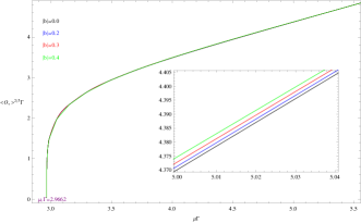
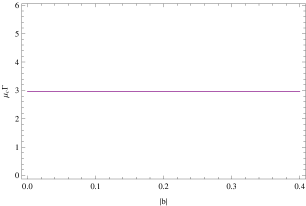
Figure 1: The condensate of operator $\langle\hat{O}_{+}\rangle$ (left plot) as a function of chemical potential $\mu$ for different parameter $b$ and the critical chemical potential $\mu_{c}$ (right plot) versus the ENE factor $b$. The different color correspond to the different value of parameter $b$.

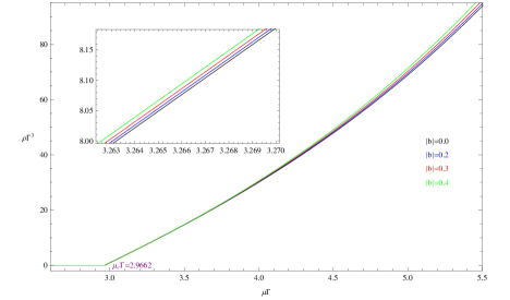
Figure 2: The charge density $\rho$ as a function of chemical potential $\mu$ for different parameter $b$, respectively. The enlarged view in the red elliptic region is plotted in the right panel. The different color correspond to the different value of parameter $b$.

Here, we plot pictures to display the explicit dependence of the chemical potential for operator $\langle\hat{O}_{+}\rangle$ and charge density $\rho$ on the ENE factor $b$. It can be seen from the Fig. 1 that there is a phase transition at the critical chemical potential $\mu_{c}$ and its value is independent of the ENE factor b which is shown in the right-hand panel. That is to say, the ENE has no effect on the critical potential of the holographic phase transition for this physical model. When $\mu<\mu_{c}$, the system is described by the AdS soliton solution itself which indicates a insulator phase turns on. When the chemical potential is bigger than the critical value $\mu_{c}$ the condensation of the operator emerges, which means the AdS soliton reaches a superconductor phase. It is interesting to find that the effect of the ENE factor $b$ on the operator in the condensate phase is not trivial. With the increase of the strength of the ENE, the value of the scalar operator becomes bigger. In Fig. 2, we note that the charge density $\rho$ in the superconductor phase drops when the ENE parameter becomes lower and the insulator/superconductor phase transition here is typically the second order in this case.

IV Holographic Entanglement Entropy

In this section, we will study the behavior of holographic entanglement entropy in this holographic model and discuss the effect of the ENE factor $b$ on the entanglement entropy. Since the choice of the subsystem $\mathcal{A}$ is arbitrary, we can define infinite entanglement entropy correspondingly. For concreteness, we investigate the holographic entanglement entropy of dual field with a half space and a belt geometry in the AdS boundary, respectively.

IV.1 Holographic Entanglement Entropy for half geometry

We first consider the subsystem $\mathcal{A}$ with a half space defined by $x>0$, $-\frac{R}{2}<y<\frac{R}{2}(R\rightarrow\infty),\ 0\leq\chi\leq\Gamma$. According to the proposal (1), the entanglement entropy can be expressed as

$$S_{\mathcal{A}}^{half}=\frac{R\Gamma}{4G_{N}}\int_{r_{0}}^{\frac{1}{\epsilon}}re^{\frac{A(r)}{2}}dr=\frac{R\pi}{8G_{N}}(\frac{1}{\epsilon^{2}}+s),$$ (20)

where $r=\frac{1}{\epsilon}$ is the UV cutoff. Note that the first term is divergent as $\epsilon\rightarrow 0$ and will not change after the operator condensationCai2012 . The second term $s$ is independent of the UV cutoff and $s=-1$ corresponds to the pure AdS soliton. As the aim of requiring the the lower bound of the integral is still equal to unit, we define a useful dimensionless coordinate in the form

$$z=\frac{r_{0}}{r}.$$ (21)

Then, the entanglement entropy for a half space can be rewritten as

$$S_{\mathcal{A}}^{half}=-\int_{1}^{\epsilon r_{0}}\frac{r_{0}^{2}e^{\frac{A(z)}{2}}}{z^{3}}dz=\frac{1}{2}(\frac{1}{\epsilon^{2}}+s),$$ (22)

while the second term $s$ is a finite term, so it is physically important. According to the scaling symmetry (17), we here choose the following scale invariants to explore physics in the entanglement entropy $s$.

$$s\Gamma^{2},\ \ \ \mu\Gamma^{2}.$$ (23)

In Fig. 3, we plot the behavior of the entanglement entropy $s$ with respect of chemical potential $\mu$ and the ENE factor $b$ in the half geometry. It can be seen from the figure that the entanglement entropy is continuous but its slop has a discontinuous change at the critical phase transition point $\mu_{c}$. Which indicates some kind of new degree of freedom like the Cooper pair would emerge after the condensation. Furthermore, the discontinuous change of the entanglement entropy at $\mu_{c}$ signals that the phase transition here is the second order transition. With the increase of the ENE factor, the value of $\mu_{c}$ dose not change. Which means the ENE parameter has no effect on the critical point of the phase transition. Before the phase transition, the entanglement entropy is a constant as we change the parameters $b$ and $\mu$ which can be interpreted as the insulator phase. After the phase transition, for a given $b$, the entanglement entropy in the superconductor phase first increases and then decreases monotonously for larger $\mu$. And the value of the entanglement entropy becomes lager as we choose a lager ENE parameter for a given $\mu$. When the factor $b\rightarrow 0$, the ENE field will reduce to the Maxwell field and our results are consistent with the one discussed in Ref.Cai2012 .

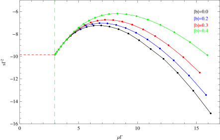
Figure 3: The entanglement entropy $s$ as a function of the chemical potential for different ENE factor $b$ in the half geometry. The red horizontal dashed line denotes the entropy in the insulator phase, the green vertical dashed line denotes the critical phase transition point where $\mu_{c}\Gamma=2.9662$ ,and the solid curves denote the entropy in the superconductor phase for various ENE factors: black curve for $|b|=0$, blue curve for $|b|=0.2$. red curve for $|b|=0.3$ and green curve for $|b|=0.4$.

IV.2 Holographic Entanglement Entropy for strip geometry

In the Following calculation, we are interested in a more nontrivial geometry which is a strip shape for region $\mathcal{A}$. We assume that the strip shape with a finite width $\ell$ along the x direction, along the $\eta$ direction with a period $\Gamma$, but infinitely extending in $y$ direction. The holographic dual surface $\gamma_{\mathcal{A}}$ defined as a codimension three surface is $t=0,\ \ x=x(r),\ \ -\frac{R}{2}<y<\frac{R}{2}\ (R\rightarrow\infty),\ \ 0\leq\chi\leq\Gamma$. Considering the surface is smooth, we suppose that the holographic surface $\gamma_{\mathcal{A}}$ starts from $x=\frac{\ell}{2}$ at $r=\frac{1}{\epsilon}$, extends into the bulk until it reaches $r=r_{*}$, then returns back to the AdS boundary $r=\frac{1}{\epsilon}$ at $x=-\frac{\ell}{2}$. The entanglement entropy of the belt geometry with connected surface in $z$ coordinate is given by

$$S^{connect}_{\mathcal{A}}[x]=-\frac{R\Gamma}{2G_{N}}\int_{z*}^{r_{0}\epsilon}\frac{r_{0}^{2}}{z^{3}}e^{\frac{A(z)}{2}}\sqrt{1+r_{0}^{2}B(z)(dx/dz)^{2}}dz,$$ (24)

where $z_{*}=r_{0}/r_{*}$ is the turning point. As the physics model is a static situation, the above Eq.(24) dose not depend on the time slice. And we could consider $S^{connect}_{\mathcal{A}}[x]$ as the integral of the Lagrangian with x direction thought of as time. Because the translations of $x$ direction is symmetry, the corresponding Hamiltonian is conserved. Therefore, the equation of motion for the minimal surface from Eq.(24) can be deduced as following

$$\frac{r_{0}^{4}B(z)(dx/dz)e^{\frac{A(r)}{2}}}{z^{3}\sqrt{1+r_{0}^{2}B(z)(dx/dz)^{2}}}=\frac{r_{0}^{3}\sqrt{B(z_{s})}e^{\frac{A(z_{s})}{2}}}{z_{s}^{3}},$$ (25)

where $z_{s}$ is a constant. And the width $\ell$ and the entanglement entropy $S$ can be easily calculated in the form

$$\frac{\ell}{2} =- \int_{z_{s*}}^{r_{0}\epsilon}\frac{1}{r_{0}\sqrt{B(z)(\frac{z_{*}^{6}B(z)e^{A(z)}}{z^{6}B(z_{*})e^{A(z_{*})})}-1)}}dz_{s},$$ (26)

$$S^{connect}_{\mathcal{A}} =- \int_{z_{s*}}^{r_{0}\epsilon}\frac{r_{0}^{2}}{z^{3}}e^{\frac{A(z)}{2}}\sqrt{1-\frac{z^{6}B(z_{*})e^{A(z_{*})}}{z_{*}^{6}B(z)e^{A(z)}}}dz+\frac{\ell}{2}\sqrt{\frac{1}{z^{6}}B(z)e^{A(z)})}r_{0}^{3}=\frac{1}{2}(\frac{1}{\epsilon^{2}}+s),$$ (27)

In addition to the solution to the connected configuration, the entanglement entropy for the disconnected geometry described two separated surfaces that are located at $x=\pm\frac{\ell}{2}$ respectively and extending to the bulk and reaching at the tip is given by

$$S_{\mathcal{A}}^{disconnect}=-\frac{R\Gamma}{2G_{N}}\int_{1}^{r_{0}\epsilon}\frac{r^{2}_{0}e^{\frac{A(z)}{2}}}{z^{3}}dz=\frac{R\pi}{4G_{N}}(\frac{1}{\epsilon^{2}}+s),$$ (28)

Here, we show in Fig. 4 the results for the entanglement entropy $s$ versus the width $\ell$ of the subsystem $\mathcal{A}$ and the ENE factor $b$ with the dimensionless quantities $s\Gamma^{2},\mu\Gamma,\ell\Gamma^{-1}$ and $b$. We find that the the discontinuous solutions represented the horizontal dotted lines in the figure is independent of the the width $\ell$ but its value of the entanglement entropy with a smaller $b$ is smaller. The connected configuration denoted by the solid lines has two solutions. Specifically, the so-called confinement/deconfinement phase transition Nishioka2007 ; Klebanov2007 ; Myers:2012ed emerges as we change the width $\ell$ and the critical value $\ell_{c}$ indicated by the vertical dotted lines becomes bigger with the increase of the parameter $b$. For a fixed $b$, in the deconfinement phase where $\ell<\ell_{c}$, considering the physical entropy determined by the choice of the lowest one, the entanglement entropy comes from the connected surface and the lowest branch in the figure is finally favored. However, the physical entanglement entropy in confinement phase where $\ell>\ell_{c}$ is dominated by the discontinuous surface and has nothing to do with the factor $\ell$. Thus, there exists four phases in the dual boundary field theory, including the insulator phase, superconductor phase and their corresponding confinement/deconfinement phases. When the parameter $\ell$ is fixed, we observe that the entanglement entropy increases as we choose a bigger ENE factor both in the confinement and deconfinement superconducting phases.

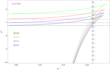
Figure 4: The entanglement entropy as a function of the strip width $\ell$ with different parameter $b$ for $\mu\Gamma=6.9165$. The black curve is for $|b|=0$ and the blue curve is for $|b|=0.2$. The red curve is for $|b|=0.3$ and the green curve is for $|b|=0.4$. The corresponding critical widths are $\ell_{c}\Gamma^{-1}=0.2109$, $\ell_{c}\Gamma^{-1}=0.2122$, $\ell_{c}\Gamma^{-1}=0.2139$, $\ell_{c}\Gamma^{-1}=0.2164$, respectively.

Interestingly, the entanglement entropy with respect to the chemical potential $\mu$ as one fixes the ENE factor $b$ or the width $\ell$ is presented in Fig. 5. At the insulator/superconductor phase transition point $\mu=\mu_{c}$, we also find that the the jump of the slop of the entanglement entropy indicates that the system undergoes the second order phase transition. Both in the confinement and deconfinement superconducting phases where $\mu>\mu_{c}$, we can see that the behavior of the entanglement entropy as a function of the chemical potential is non-monotonic and similar to the case in the half geometry which we have discussed above. As the chemical potential is fixed, the value the entanglement entropy becomes smaller when the factors $b$ and $\ell$ become lower. More specifically, the the effect of the ENE factor on the entanglement entropy is weaker than the width of the subsystem $\mathcal{A}$. In their corresponding insulator phases where $\mu<\mu_{c}$, we observe that the value of the entanglement entropy does not change as we alter the parameter $b$ for a given $\mu$. On the other hand, with the increase of the width the entanglement entropy increases. That is to say, the behavior of the entanglement entropy in the corresponding insulator phases is independent of the the ENE factor but depends on the the width of the subsystem $\mathcal{A}$.

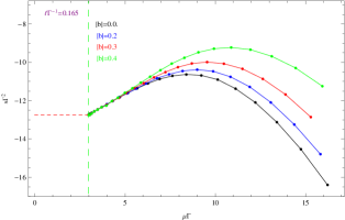
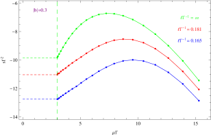
Figure 5: The entanglement entropy $s$ as a function of the chemical potential $\mu$ for the various factors,i.e., the ENE factor $b$ and the belt width $\ell$. The horizontal dotted lines denote the entropy in the insulator phase, the green vertical dashed line denotes the critical phase transition point where $\mu_{c}\Gamma=2.9662$, and the solid curves denote the entropy in the superconductor phase. The left-hand figure corresponds to $\ell\Gamma^{-1}=1$ and different b: black curve for $|b|=0$ , blue curve for $|b|=0.2$, red curve for $|b|=0.3$ and green curve for $|b|=0.4$. The right-hand figure corresponds to $|b|=0.3$ and different $\ell$: green curve for $\ell\Gamma^{-1}=\infty$, red curve for $\ell\Gamma^{-1}=0.181$ and blue one for $\ell\Gamma^{-1}=0.165$.

IV.3 phase diagram

Finally, according to our calculation for entanglement entropy in holographic insulator/superconductor transition with ENE field, we use a picture to display the phase diagram of entanglement entropy with a straight geometry.

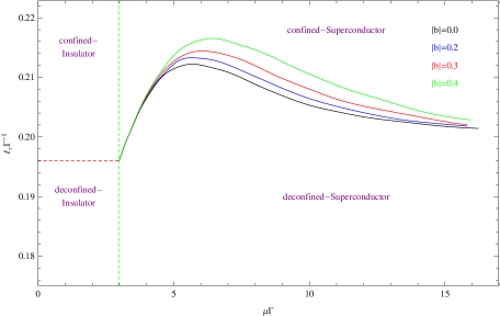
Figure 6: The phase diagram of the entanglement entropy for a strap geometry in the holographic insulator/superconductor transition with ENE field. The black curve is for $|b|=0$ and the blue curve is for $|b|=0.2$. The red curve is for $|b|=0.3$ and the green curve is for $|b|=0.4$.

In Fig. 6, the insulator phase and the superconductor phase are separated by the green vertical dashed line and the phase boundary between the confinement phase and the deconfinement phase is separated by the red horizontal dashed line and the solid curve. Therefore, the phases characterized by the parameters $\mu$ and $\ell$ contain the insulator phase, superconductor phase and their corresponding confinement/deconfinement phases. It can be clearly seen from the figure that the critical width $\ell_{c}$ of the confinement/deconfinement phase transition in the insulator phase is independent of the ENE parameter. In the superconductor phase, however, the critical width $\ell_{c}$ increases with the increase of the ENE factor. To further study, we observe that the critical width $\ell_{c}$ has a non-monotonic change as the chemical potential becomes bigger. Concretely, the entanglement entropy first increases beyond the cusp at the certain chemical potential, reaches to a maximum and decreases to a minimum, and then approaches a plateau at very large $\mu$.

V Summary

We have studied the properties of phase transitions by calculating the behaviors of the scalar operator and the entanglement entropy in holographic insulator/superconductor model with ENE. On the basis of the behaviors of the scalar operator in this holographic model, we find that there is a insulator/superconductor transition at the critical chemical potential point and the effect of the ENE factor on the scalar condensation is quite different from those observed in the holographic metal/superconductor transition with ENE field modelYao2016 . Specifically, in the holographic insulator/superconductor system the ENE factor does not have any effect on the critical chemical potential of the transition. These conclusions can also be understood from the behavior of the entanglement entropy. From the Fig. 3, the discontinuity of the slop of the entanglement entropy in half space at the critical chemical potential point signals some kind of new degree of freedom like the Cooper pair would emerge after the condensation and indicates the order of associated phase transition in the system. In Fig. 5, we observed the behavior of the entanglement entropy with respect chemical potential in strip geometry at the insulator/superconductor transition point is similar to the half case. That is to say, the entanglement entropy is indeed a good tool to search for the phase transition point.

In the superconducting phase, compared to the phenomenon observed in the scalar operator, the entanglement entropy versus the chemical potential displays more rich behaviors. Both in the half space and the belt space, the non-monotonic behavior of the entanglement entropy versus the chemical potential is general in this model as the ENE parameter is fixed. For a given chemical potential, the value the entanglement entropy becomes smaller when the ENE factor or the with becomes lower. In the insulator phase, however, the behavior of entanglement entropy is independent of the the ENE parameter.

Interestingly, considering the the effect of the belt width on the entanglement entropy, we obtained that the confinement/deconfinement phase transition appears in both insulator and superconductor phases and the complete phase diagram of the entanglement entropy with a straight geometry is presented in Fig. 6. It is shown that the critical width of the the confinement/deconfinement phase transition depends on the chemical potential and the ENE term.

- (1) J. M. Maldacena, The large N limit of superconformal field theories andsupergravity Adv. Theor. Math. Phys. 2, 231-252 (1998). [hep-th/9711200].
- (2) S. S. Gubser, I. R. Klebanov, Gauge theory correlators from noncritical string theory, A. M. Polyakov, Phys. Lett.B 428, 105-114 (1998). [hep-th/9802109].
- (3) E. Witten, Anti-de Sitter space and holography, Adv. Theor. Math. Phys. 2, 253-291 (1998). [hep-th/9802150].
- (4) S. A. Hartnoll, C. P. Herzog and G. T. Horowitz, Building a Holographic Superconductor, Phys. Rev. Lett. 101, 031601 (2008).
- (5) S. A. Hartnoll, C. P. Herzog and G. T. Horowitz, Holographic superconductors, JHEP 12, 015 (2008).
- (6) G. T. Horowitz and M. M. Roberts, Holographic Superconductors with Various Condensates, Phys. Rev. D 78 , 126008 (2008)
- (7) S. A. Hartnoll, Lectures on holographic methods for condensed matter physics, Class. Quant. Grav.26, 224002 (2009).
- (8) G. T. Horowitz, Introduction to holographic superconductors, arXiv: 1002.1722 [hep-th].
- (9) Gary T.Horowitz, Benson Way Complete Phase Diagrams for a Holographic Superconductor/Insulator System, JHEP 1011, 011 (2010).
- (10) Jiliang Jing and Songbai Chen, Holographic superconductors in the Born-Infeld electrodynamics, Phys. Lett. B 686, 68 (2010); Jiliang Jing, Qiyuan Pan, Songbai Chen, Holographic Superconductors with Power-Maxwell field, JHEP 11, 045 (2011).
- (11) Yan Peng, Qiyuan Pan, Bin Wang, Various types of phase transitions in the AdS soliton background, Phys.Lett.B 699:383-387 (2011).
- (12) Sunandan Gangopadhyay, Dibakar Roychowdhury, Analytic study of properties of holographic superconductors in Born-Infeld electrodynamics, JHEP 05, 002 (2012).
- (13) Zixu Zhao, Qiyuan Pan, Songbai Chen, Jiliang Jing, Notes on holographic superconductor models with the nonlinear electrodynamics, Nucl. Phys. B 98, 871 [FS] (2013).
- (14) Sunandan Gangopadhyay, Dibakar Roychowdhury, Analytic study of Gauss-Bonnet holographic superconductors in Born-Infeld electrodynamics, JHEP05, 156 (2012).
- (15) Jiliang Jing, Qiyuan Pan, Songbai Chen, Holographic Superconductor/Insulator Transition with logarithmic electromagnetic field in Gauss-Bonnet gravity, Phys. Lett. B 716, 385 (2012).
- (16) Weiping Yao, Jiliang Jing, Analytical study on holographic superconductors for Born-Infeld electrodynamics in Gauss-Bonnet gravity with backreaction, JHEP 05, 101 (2013).
- (17) Shirsendu Dey, Arindam Lala, Holographic s-wave condensation and Meissner-like effect in Gauss-Bonnet gravity with various non-linear corrections, Annals of Physics 354, 165-182 (2015).
- (18) Chuyu Lai, Qiyuan Pan, Jiliang Jing, and Y. Wang, On analytical study of holographic superconductors with Born- Infeld electrodynamics, Phys. Lett. B 749, 437 (2015).
- (19) Hamid Reza Salahi, Ahmad Sheykhi, Afshin Montakhab, Effects of Backreaction on Power-Maxwell Holographic Superconductors in Gauss-Bonnet Gravity, Eur. Phys. J. C 76, 575 (2016).
- (20) Zeinab Sherkatghanad, Behrouz Mirza, Fatemeh Lalehgani Dezaki,Exponential nonlinear electrodynamics and backreaction effects on Holographic superconductor in the Lifshitz black hole background, International Journal of Modern Physics D, 26, 1750175 (2017).
- (21) A. Sheykhi, F. Shamsi, Holographic Superconductors with Logarithmic Nonlinear Electrodynamics in an External Magnetic Field, Int J Theor Phys 56, 916 (2017). Ahmad Sheykhi, Fatemeh Shaker, Effects of backreaction and exponential nonlinear electrodynamics on the holographic superconductors, Journal of Modern Physics D26, 1750050 (2017). Ahmad Sheykhi, Afsoon Ghazanfari, Amin Dehyadegari, Holographic conductivity of holographic superconductors with higher order corrections, Eur. Phys. J. C 78, 159 (2018)
- (22) S. Ryu and T. Takayanagi, Holographic derivation of entanglement entropy from AdS/CFT, Phys. Rev. Lett. 96, 181602 (2006).
- (23) S. Ryu and T. Takayanagi, Aspects of Holographic Entanglement Entropy, JHEP 0608, 045 (2006).
- (24) D. V. Fursaev, Proof of the holographic formula for entanglement entropy, JHEP 0609, 018 (2006).
- (25) T. Hirata and T. Takayanagi, AdS/CFT and strong subadditivity of entanglement entropy, JHEP 0702, 042 (2007).
- (26) T. Nishioka and T. Takayanagi, AdS Bubbles, Entropy and Closed String Tachyons, JHEP 0701, 090 (2007).
- (27) I. R. Klebanov, D. Kutasov and A. Murugan, Entanglement as a probe of confine- ment, Nucl. Phys. B 796, 274 (2008).
- (28) R. C. Myers and A. Singh, Comments on Holographic Entanglement Entropy and RG Flows, JHEP 1204, 122 (2012).
- (29) A. Pakman and A. Parnachev, Topological Entanglement Entropy and Holography, JHEP 0807, 097 (2008).
- (30) T. Albash and C. V. Johnson, Holographic Studies of Entanglement Entropy in Superconductors, JHEP 05, 079 (2012).
- (31) Rong-Gen Cai, Song He, Li Li, Yun-Long Zhang, Holographic Entanglement Entropy in Insulator/Superconductor Transition, JHEP 1207, 088 (2012).
- (32) Rong-Gen Cai, Song He, Li Li, Li-Fang Li, Entanglement Entropy and Wilson Loop in Stš¹ckelberg Holographic Insulator/Superconductor Model, JHEP 1210, 107 (2012). Rong-Gen Cai, Li Li, Li-Fang Li, Ru-Keng Su, Entanglement Entropy in Holographic P-Wave Superconductor/Insulator Model, JHEP 1306, 063 (2013).
- (33) J. de Boer, M. Kulaxizi and A. Parnachev, “Holographic Entanglement Entropy in Lovelock Gravities,” JHEP 1107, 109 (2011).
- (34) L. -Y. Hung, R. C. Myers and M. Smolkin, “On Holographic Entanglement Entropy and Higher Curvature Gravity,” JHEP 1104, 025 (2011).
- (35) N. Ogawa and T. Takayanagi, “Higher Derivative Corrections to Holographic Entanglement Entropy for AdS Solitons,” JHEP 1110, 147 (2011).
- (36) Xi Dong, Holographic Entanglement Entropy for General Higher Derivative Gravity, JHEP 01, 044 (2014).
- (37) Xiao-Mei Kuang, Eleftherios Papantonopoulos, Bin Wang, Entanglement Entropy as a Probe of the Proximity Effect in Holographic Superconductors, Journal of High Energy Physics 1405, 130 (2014).
- (38) Yan Peng, Holographic entanglement entropy in superconductor phase transition with dark matter sector, Physics Letters B 750: 420-426 (2015).
- (39) Xiao-Xiong Zeng, Hongbao Zhang, Li-Fang Li, Phase transition of holographic entanglement entropy in massive gravity, Physics Letters B 756 ,170 (2016).
- (40) N.S. Mazhari, D. Momeni, R. Myrzakulov, H. Gholizade, M. Raza, Non-equilibrium phase and entanglement entropy in 2D holographic superconductors via Gauge-String duality, Canadian Journal of Physics 10, 94 (2016).
- (41) Yan Peng, Guohua Liu, Holographic entanglement entropy in two-order insulator/superconductor transitions, Physics Letters B 767:330-335 (2017).
- (42) Weiping Yao, Jiliang Jing, Holographic entanglement entropy in insulator/superconductor transition with Born-Infeld electrodynamics, JHEP 05,058 (2014).
- (43) Weiping Yao, Jiliang Jing, Holographic entanglement entropy in metal/superconductor phase transition with Born-Infeld electrodynamics, Nuclear Physics B 889, 109 (2014).
- (44) Yunqi Liu, Yungui Gong, Bin Wang, Non-equilibrium condensation process in holographic superconductor with nonlinear electrodynamics, JHEP 02, 116 (2016).
- (45) M. Born, L. Infeld, Foundations of the New Field Theory, Proc. R. Soc. A 144 (1934) 425.
- (46) S.H. Hendi, Asymptotic charged BTZ black hole solutions, J. High Energy Phys. 03, 065 (2012).
- (47) S. H. Hendi, A. Sheykhi, Charged rotating black string in gravitating nonlinear electromagnetic fields, Phys. Rev. D 88, 044044 (2013).
- (48) M. Born and L. Inleild, Foundations of the New Field Theory, Proc. R. Soc. A. 144, 425 (1934).
- (49) B. Hoffmann, Gravitational and Electromagnetic Mass in the Born-Infeld Electrodynamics, Phys. Rev. 47, 877 (1935).
- (50) W. Heisenberg and H. Euler, Folgerungen aus der Diracschen Theorie des Positrons, Z. Phys. 98 714, (1936).
- (51) H. P. de Oliveira, Non-linear charged black holes, Class. Quant. Grav. 11, 1469 (1994).
- (52) G. W. Gibbons and D. A. Rasheed, Electric-magnetic duality rotations in non-linear electrodynamics, Nucl. Phys. 454, 185 (1995).
- (53) S. H. Hendi, Asymptotic Reissner-Nordstrom black holes, Annals of Physics (N.Y.) 333, 282 (2013). S. H. Hendi, Thermodynamic properties of asymptotically Reissner-Nordstrom black holes, Annals of Physics 346, 42-50 (2014).
- (54) S. H. Hendi, A. Sheykhi, M. Sepehri Rad, K. Matsuno, Slowly rotating dilatonic black holes with exponential form of nonlinear electrodynamics , Gen. Rel. Grav. 47, 117 (2015).
- (55) A. Sheykhi, S. Hajkhalili Dilaton black holes coupled to nonlinear electrodynamic field, Phys. Rev. D 89, 104019 (2014).
- (56) A. Sheykhi, A. Kazemi Higher dimensional dilaton black holes in the presence of exponential nonlinear electrodynamics, Phys. Rev. D 90, 044028 (2014).
- (57) M. Kord Zangeneh, A. Dehyadegari, A. Sheykhi, M. H. Dehghani, Thermodynamics and gauge/gravity duality for Lifshitz black holes in the presence of exponential electrodynamics, JHEP 1603, 037 (2016).
- (58) S.I. Kruglov, Corrections to Reissner-Nordstr?m black hole solution due to exponential nonlinear electrodynamics, Europhys. Letters, 115, 60006 (2016). S. I. Kruglov, Black hole as a magnetic monopole within exponential nonlinear electrodynamics, Ann. Phys., 378, 59 (2017).
- (59) S. Hajkhalili, A. Sheykhi, Asymptotically (A)dS dilaton black holes with nonlinear electrodynamics, arXiv:1801.05697.
- (60) V. A. De Lorenci, R. Klippert, M. Novello, and J. M. Salim Nonlinear electrodynamics and FRW cosmology Phys. Rev. D 65, 063501 (2002).
- (61) M. Novello, S. E. Perez Bergliaffa, and J. Salim, Nonlinear electrodynamics and the acceleration of the Universe Phys. Rev. D 69, 127301 (2004)
- (62) M. Novello, A.N. Araujo, J.M. Salim The cosmological origins of nonlinear electrodynamics, Int. J. of Mod. Phys. A 24, 5639 (2009).
- (63) Weiping Yao, Jiliang Jing, Holographic entanglement entropy in metal/superconductor phase transition with exponential nonlinear electrodynamics, Phys. Lett. B 759, 533 (2016).
- (64) P. Breitenlohner and D. Z. Freedman, Stability In Gauged Extended Supergravity, Annals Phys. 144, 249 (1982). P. Breitenlohner and D. Z. Freedman, Positive Energy In Anti-De Sitter Backgrounds And Gauged Extended Supergravity, Phys. Lett. B 115, 197 (1982).