Day-ahead Trading of Aggregated Energy Flexibility - Full Version

Abstract.

Flexibility of small loads, in particular from Electric Vehicles (EVs), has recently attracted a lot of interest due to their possibility of participating in the energy market and the new commercial potentials. Different from existing work, the aggregation techniques proposed in this paper produce flexible aggregated loads from EVs taking into account technical market requirements. They can be further transformed into the so-called flexible orders and be traded in the day-ahead market by a Balance Responsible Party (BRP). As a result, the BRP can achieve at least $20$% cost reduction on average in energy purchase compared to traditional charging based on 2017 real electricity prices from the Danish electricity market.

1. Introduction

The integration of EVs into the Smart Grid reveals new business opportunities by exploiting their inherent flexibility (Hu et al., 2016; Kristoffersen et al., 2011). A market actor that controls the charging rate and time of a portfolio of EVs could acquire financial gain from energy arbitrage (Cao et al., 2012; Biegel et al., 2014). The energy required to charge (and/or discharge) the EVs can be traded through bids in day-ahead and/or regulation market at a minimum cost (Sarker et al., 2016). Numerous research studies, European (e.g., (mir, 2012), and national projects (e.g., (tot, 2015)) focus on trading the required energy to charge EVs taking into account different parameters.

An optimization charging approach of EVs that activates the participation in both day-ahead and regulation markets is proposed in (Bessa et al., 2012). Scheduling techniques of EV charging that aim to maximize the market actor’s profit and take into account electricity price uncertainty are suggested in (Vandael et al., 2015) and (Zhao et al., 2017). A risk-based scheduling framework for charging EVs is also proposed in (Yang et al., 2014). The suggested algorithm is based on day-ahead prices and takes into account driving activity uncertainties in order to minimize the charging cost of the EVs. Similarly, a day-ahead optimization technique for scheduling EVs considering the impact on the day-ahead prices is suggested in (Liu et al., 2017). Both optimization and heuristic techniques for optimal charging of EVs aiming to the maximization of the revenue by utilizing energy storage are proposed in (Jin et al., 2013).

The main characteristic of the research tackling the energy trading of flexible EV loads is the output of the proposed techniques, i.e., an aggregated scheduled load. Unlike other work, we introduce $3$ aggregation techniques that produce flexible aggregated loads that can be traded in the market. As a result, the market itself, not the market actors, schedules the loads from the EVs as part of the trading process, minimizing the uncertainty of bidding. For instance, instead of placing a bid to purchase $30$MW in hour $3$, the market actor places a bid to purchase $30$MW in any hour between hour $1$ and $5$. The market determines the activation time of the bid. In many cases, the technical trading details of the market impose hard constraints that are omitted by the proposed solutions and the realization of the suggested techniques becomes very difficult. For instance, the proposed scheduling technique in (de Cerio Mendaza et al., 2016) offers less than $200$kW in less than an hour in the regulation power market where the minimum bid is $10$MW, in full hours (Biegel et al., 2014). The bidding strategies proposed in (Baringo and Amaro, 2017) and the high power fluctuations of the scheduling outputs in (Bessa et al., 2012) and in (Sarker et al., 2016), would require single hour independent bids (Nor, 2017) that might not fulfill the energy requirements. The conservative bidding approach for the bidding strategy proposed in (Vaya and Andersson, 2015) covers less than 50% of the energy needed to charge the EVs. On the contrary, our proposed aggregation techniques use real technical market requirements derived from a specific order (bid) type of Nordic market, namely, flexible orders (Nor, 2017).

Contributions. First, we describe both the so-called flex-offer (FO) model, which captures the flexibility of the EVs, and a realistic market framework where the flexibility is traded. Second, we investigate the market-based FO aggregation problem and its complexity. Third, we introduce $3$ heuristic algorithms that take into account real market requirements and produce flexible aggregated FOs that can be then traded through flexible orders in the market. Finally, we compare our proposed techniques with $2$ base-line approaches and evaluate both the technical and the financial aspect of their results based on real market prices. We show that our proposed techniques achieve more than $20$% cost reduction on average in the purchased energy required to charge from $5$K to $40$K EVs.

The paper is organized as follows: we introduce the preliminary definitions in Section 2 and we present the problem formulation of market-based aggregation in Section 3. In Section 4, we propose $3$ heuristic market-based aggregation techniques and we experimentally evaluate them in Section 5. We conclude the paper in Section 6.

2. Preliminaries

In this section, we describe the EV model that can be used to trade flexibility and the market framework used for trading.

2.1. Electric vehicle model

We consider the energy used to charge EVs to be appropriate for flexible energy trading. The reason is that the lithium-ion batteries of EVs are ample power demand devices and their charge can be time shifted when the EVs are plugged-in for more hours than needed for charging. We consider EVs that can be continuously charged with a power-constant voltage (CP-CV) option (Vagropoulos et al., 2016) and their charge is taking place in the range of 20% to 90% state of charge (SOC) so that the battery life is preserved (Marra et al., 2012). As a result, when an EV is plugged in for charging, its battery capacity is at least 20% and the user would like to fully charge it (90%) for his/her next trip. The SOC is computed according to the following formula based on (Vagropoulos et al., 2016): $\mathit{SOC_{final}}=\mathit{SOC_{ini}}+\frac{\eta_{c}\cdot\eta_{b}\cdot P\cdot time_{cha}}{C}$ (1) where $\mathit{SOC_{final}}$ is the final state of charge equal to 90% of the total battery capacity ($C$). Parameters $\eta_{c}$ and $\eta_{b}$ represent the efficiency of the charger and the internal resistance of the battery, respectively. We represent with $P$ the power used to charge an EV that is constant over the [20%, 90%] interval of SOC and $time_{cha}$ is the time needed to charge it up to $\mathit{SOC_{final}}$.

In our work, because we take into account time shifted loads, we use the flex-offer (FO) concept (Siksnys et al., 2015), introduced in the MIRABEL project (mir, 2012; Boehm et al., 2012) to represent the charging of a flexible EV. An FO captures flexibility from different dimensions (e.g., time, energy, and/or combined) (Valsomatzis et al., 2015), from different devices (Šikšnys and Pedersen, 2016), and can be used for different purposes, e.g., tackle electrical grid bottlenecks (Valsomatzis et al., 2016). Thus, we define an FO $f$ to be a tuple $f=(T(f),P(f))$ where $T(f)$ is the start charging flexibility interval and $P(f)$ is the power profile. $T(f)=[t_{es},t_{ls}]$ where $t_{es}$ and $t_{ls}$ are the earliest start charging time and latest start charging time, respectively. We define time flexibility ($\mathit{tf}$) to be the difference between $t_{ls}$ and $t_{es}$. The power profile is a sequence of ($m\in\mathbb{N}_{>0}$) consecutive slices, $P(f)=\langle s^{(1)},\dots,s^{(m)}\rangle$ where a slice $s^{(i)}$ has a power value $p$ measured in kW. The duration of slices is 1 hour.

For instance, an EV is plugged in at a house between $1$ and $8$ a.m. The EV continuously utilizes $3.7$kW for $3.3$ hours to be charged. However, energy trading is performed per hour and we also use hourly resolution to model the EVs charging. To respect the hourly granularity, we equally distribute the sum of the energy needed during the first and the last regular charging hours and we reduce power fluctuations in the model. Therefore, we assume that the EV consumes $2.4$kWh both during the first and the last charging hours and $3.7$kWh during the hours in-between. The EV can be modeled by an FO $f$$=$$([1,4],\langle 2.4,3.7,3.7,2.4\rangle)$, see Figure 1a. Next, we describe the market framework where such FOs shall be traded.

2.2. Market framework

The Nordic/Baltic market for electrical energy named Nord Pool is considered in our work. Nord Pool is one of the most mature energy markets (Weron, 2006) and Europe’s leading power market (Nor, 2017). It consists of the day-ahead (Elspot) and intra-day markets. We focus on Elspot because it has one of the largest turnovers in the Nordic system and it also supports flexible energy trading (Biegel et al., 2014). Trading in Elspot occurs daily through orders (bids). Each day before 12 p.m., the balance responsible parties (BRPs) place their purchase and/or selling orders (bids) in Elspot for the following day. The orders specify the energy amount a BRP desires to buy/sell and the price the BRP is willing to pay/be paid for the corresponding energy. Since 2016, Elspot supports 4 different order types: single hourly orders (price dependent or independent), block orders, exclusive groups, and flexible orders (Nor, 2017). We focus on flexible orders that support flexibility trading.

When a BRP places a flexible order in Elspot, it states the name, the time interval, the price limit, the volume, and the duration of the order. The time unit is one hour and volume is expressed in MW. The duration expresses the number of hours during which the order can be activated over the interval $[1,23]$. The time interval must exceed the duration by at least one hour and expresses the potential activation times of the order. Volume is either positive, if the order is a purchase order or negative, if it is a sell order. A BRP can place $5$ flexible orders during a trading day.

Hypothetically, a BRP could purchase the energy needed to charge the above mentioned flexible EV, represented by FO $f$ through a flexible order. The duration of a flexible order is mapped to the number of slices of $f$, the volume to the power of the slices, and the time interval to the time flexibility of $f$. For instance, a BRP could place a flexible order named “F1”, with duration $4$ hours and time interval from $1$ to $8$. The volume of F1 is $0.0037$MW (in order to satisfy all the slices) and its price limit is 35 euros/MWh. However, the energy needed to charge a single EV is (much) too small to be traded in Elspot. In particular, the minimum contract size and the volume trade lot for a flexible order are both $100$kW, while the power used by an EV is a few kW. Moreover, when the duration of a flexible order is more than one hour, the volume needed for these hours shall be constant. As a result, it is necessary to aggregate FOs to trade the flexible loads of the EVs through flexible orders in Elspot market.

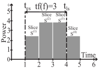
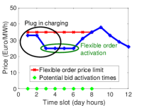
(a)	(b)

Figure 1. An examle of an FO and a flexible purchase order

The flexible order is activated in the time interval that optimizes social welfare provided that the price is respected (Nor, 2017). Given F1 in a liquid market, the order is activated when the cost of buying the required energy is minimized. For instance, we see in Figure 1b that F1 is activated in time slots $3$, $4$, $5$, and $6$ where the price is $25$ euros/MWh. Thus, the energy needed to charge the EV costs $25\cdot 0.0037\cdot 4=0.37$ euros. On the contrary, if time flexibility of the EV is disregarded, its charging occurs based on a price independent order and its plug-in time (time slot $1$-$4$ in Figure 1b). As a result, the energy needed to charge the EV is purchased based on a price independent order and the price is set by Elspot. In that case and according to Figure 1b, the cost is $33\cdot 0.0037\cdot 2+25\cdot 0.0037\cdot 2=0.4292$ euros, $16$% more than the cost achieved by flexible order F1. Therefore, a flexible order has a higher probability to achieve a better price than a price independent order because it takes into account the time flexibility of the flexible loads and thus can be favored by price reductions. The absolute difference (imbalance) between the purchased energy and the energy needed is traded in the balance market and usually for a higher price than the one in Elspot. Consequently, the BRP desires to be as precise as possible regarding the purchased energy from Elspot.

Regarding the communication among an EV and a BRP, we assume an Information and Communication Technology (ICT) infrastructure (Albano et al., 2015). When an EV is plugged in, an FO is generated requiring the minimum interaction with the owner of the EV. The FO generation takes into account the historical use of the EV, the $\mathit{SOC_{ini}}$ of the EV, the charging characteristics of the EV, and the technical characteristics of the charging station, e.g., a home charging installation (Neupane et al., 2017). Identifying the time flexibility of an FO is challenging, but appropriate forecast techniques can be designed taking into account daily/weekly driving patterns (Bessa and Matos, 2012).

3. Problem Formulation

In this section, we show how aggregation of FOs that represent flexible charging loads of EVs can fulfill the requirements of flexible orders. We also introduce the problem of market-based aggregation.

3.1. FO aggregation

Based on (Siksnys et al., 2015), FO aggregation is the function that given a set of FOs $F$, produces a set of aggregated FOs $\mathit{AF}$ where $\mathit{|AF|}\leq|F|$. The produced AFOs capture large amounts of energy that can be traded in the market. Due to the time flexibility of the FOs, there are different alignment combinations that can lead to different AFOs. According to start-alignment FO aggregation, the earliest start charging time of an aggregated FO (AFO) $f_{a}$ is the minimum earliest start charging time among all the FOs that produced it, i.e., $f_{a}.t_{es}=min_{f\in F^{\prime}}(f.t_{es}),F^{\prime}\subseteq F$. The latest start charging time of $f_{a}$ is the sum of its $t_{es}$ and the minimum time flexibility among all the FOs in $F^{\prime}$, i.e., $f_{a}.t_{ls}=f_{a}.t_{es}+min_{f\in F^{\prime}}(tf(f))$. The power profile of $f_{a}$ is produced by summing up the power profiles of the FOs when they are aligned according to their earliest start charging time.

For instance, we see in Figure 2a three FOs, $f_{1}=([1,5],\langle 1,1\rangle)$ $f_{2}=([2,3],\langle 1,1\rangle)$, and $f_{3}=([4,5],\langle 1\rangle)$, that produce AFO $f_{123}$ where $f_{123}.t_{es}=f_{1}.t_{es}=1$ and $f_{123}.t_{ls}$ is the sum of $f_{123}.t_{es}$ and time flexibility of $f_{2}$ or $f_{3}$, i.e., $f_{123}.t_{ls}=2$. The power profile of $f_{123}$ is produced by summing up the power profiles of $f_{1}$, $f_{2}$, and $f_{3}$ based on their alignments. Thus, $f_{123}.s^{(1)}.p=f_{1}.s^{(1)}.p=1$, $f_{123}.s^{(2)}.p=f_{1}.s^{(2)}.p+f_{2}.s^{(1)}.p=2$, $f_{123}.s^{(3)}.p=f_{2}.s^{(2)}.p=1$, and $f_{123}.s^{(4)}.p=f_{3}.s^{(1)}.p=1$.

Due to the time flexibility of the FOs, there are different alignment combinations that can lead to different AFOs. For instance, given the $3$ FOs $f_{1},f_{2},f_{3}$ in Figure 2 with time flexibility 4, 1, and 1, respectively, there are 20 $(5\cdot 2\cdot 2)$ alignment combinations. As a result, based on different alignments, time flexibility of the FOs can be adjusted accordingly and different power profiles for the AFOs are produced.

Figure 2. Flex-offer aggregation according to different alignments

Moreover, a set of FOs can be partitioned and each subset can produce an AFO. Consequently, the output size of aggregation can be greater than one. For instance, we see in Figure 2b that the output of aggregation is $2$ AFOs, i.e., $f_{12}$ and $f_{3}$. In particular, FO $f_{1}$ is aligned with $f_{2}$ and time flexibility of $f_{1}$ is adjusted so that $f_{1}.t^{\prime}_{es}$ is equal to $f_{2}.t_{es}$. Consequently, the power profiles of $f_{1}$ and $f_{2}$ are summed up and they produce AFO $f_{12}$.

3.2. Market-based FO aggregation

Given a portfolio, the goal of a BRP is to maximize its profit by purchasing, for the minimum price, the energy that it sells to its customers. We consider flexible EVs to be part of a BRP’s portfolio and, since the energy purchase takes place through orders, we examine if the energy needed to charge the flexible EVs can be purchased through flexible orders. The purchasing strategy of a BRP depends on many different factors, e.g., the content of the portfolio (factories, households, etc.) and pricing forecast. The strategy is out of scope of this work and left for Future work. However, since a flexible order has in general a higher probability to achieve a lower purchase price, we consider the goal of a BRP to be the maximization of the purchased energy through flexible orders. In our work, we introduce market-based FO aggregation (MAGG) to be the aggregation that given a set of FOs, outputs between one and five AFOs that fulfill the flexible order requirements, see Equations (1a)–(1b). AFOs summarize the energy requirements and flexibilities in amount and time imposed by the technical requirements of a flexible order.

In order for an FO to fulfill the flexible order requirements, the FO must have ($1$) time flexibility at least one (Equation (1c)) and ($2$) between $1$ and $23$ slices (Equation (1d)). Moreover, since the minimum contract size and the trade lot of a flexible order are both $100$kW, ($3$) the values of the slices of the FOs shall be multiples of $100$kW.

For illustrating purposes, we assume in our example below that both the volume and the trade lot for a flexible order is $2$kW instead of $100$kW. For instance, we see in Figure 2 that none of the individual FOs fulfills the power profile requirements of a flexible order ($2$kW). Thus, market-based FO aggregation is necessary. In that case, market-based FO aggregation produces AFO $f_{12}$ that fulfills the flexible-order requirements since its time flexibility is 1 and the power of both the slices equals to 2, see Figure 2b. FO $f_{3}$ is also part of the aggregation output, but it is not a valid AFO because it does not fulfill the power profile requirement, i.e., its slice amount is lower than 2.

The flexible EVs are represented by a set of FOs. For instance, $5000$ EVs that are part of a BRP’s portfolio are represented by a set of FOs $F$. Each EV is an FO $f$ of the set, i.e., $f\in F,f=(T(f),P(f)),T(f)=[t_{es},t_{ls}],P(f)=\langle s^{(1)},\dots,s^{(m)}\rangle$. A BRP must aggregate the FOs to produce AFOs that fulfill the flexible order requirements and can be then placed in the market as flexible orders. The volume of energy is expressed through the sum of the slices of the FOs and the power of each slice must be a multiple of 100kW (Equation (1f)). However, due to technical charging characteristics (EV power demand is in the interval [3.7kW,11kW] for household charging), we take into account a power range to define the valid power amounts. Thus, instead of considering exact multiples of $100$kW for the power amount of each slice, we permit an insignificant amount deviation of $e$kW per slice, e.g., $5$kW (Equation (1f)). When the financial evaluation of market-based aggregation occurs, the deviated amount will be considered to be traded in balance market, see Section 2.2. Hence, the problem of maximizing the bidden energy through flexible orders given a set of FOs is formulated as follows:

(1a) Maximize $$\sum_{f_{a}\in\mathit{AF}}\sum_{s\in P(f_{a})}s.p$$

(1b) subject to $$\mathit{AF}=\mathit{MAGG(F)},1\leq|\mathit{AF}|\leq 5$$

(1c) $$\forall f_{a}\in\mathit{AF},\mathit{tf(f_{a})}\geq 1$$

(1d) $$\forall f_{a}\in\mathit{AF},1\leq|P(f_{a})|\leq 23$$

(1e) $$\forall f_{a}\in\mathit{AF},\forall s\in P(f_{a}),$$

(1f) $$s.p=x\cdot 100\text{kW}\pm e\text{kW},x\in\mathbb{N}_{>0},e\in[0,5]$$

3.3. Market-based FO aggregation complexity.

Given a set of FOs $F$, there are $\genfrac{\{}{\}}{0.0pt}{}{|F|}{k}$ ways (Stirling numbers of the second kind (Graham, 1994)) to partition the $|F|$ FOs into $k$ subsets. Applying aggregation on each subset produces an AFO. In market-based FO aggregation, the size of the output is between $1$ and $5$. Thus, $k$ can be assigned values from $1$ to $5$. Therefore, there are $\genfrac{\{}{\}}{0.0pt}{}{|F|}{1}$ ways to partition $|F|$ FOs into $1$ non-empty subset of FOs. There are $\genfrac{\{}{\}}{0.0pt}{}{|F|}{2}$ ways to partition the $|F|$ FOs into $2$ non-empty subsets, where the aggregated FOs are $2$ and so on. Thus, given $|F|$ FOs, there are $\genfrac{\{}{\}}{0.0pt}{}{|F|}{1}+\genfrac{\{}{\}}{0.0pt}{}{|F|}{2}+\dots+\genfrac{\{}{\}}{0.0pt}{}{|F|}{5}=\sum_{k=1}^{5}\genfrac{\{}{\}}{0.0pt}{}{|F|}{k}$ ways to partition the FOs.

Moreover, the number of the different aggregated FOs depends on the alignments of the FOs and thus on their time flexibility. In particular, given a set of FOs $\mathit{SF}$ ($\mathit{SF}$$\subseteq$$F$) with time flexibility $\mathit{tf(f_{1}),\dots,tf(f_{|\mathit{SF}|})}$ respectively, the number of the aggregation results (aggregated FOs) that can be produced is: $\prod_{i=1}^{|\mathit{SF}|}\mathit{tf(f_{i})}$. Hence, given an average number of partitions ($\mathit{avg(al)}$), there are $\sum_{k=1}^{5}\genfrac{\{}{\}}{0.0pt}{}{|F|}{k})\times\mathit{avg(al)}$ potential aggregation results. Furthermore, the complexity of the problem, as an Integer Linear Programming problem, is too high to be solved by state-of-the-art solvers (Mittelmann, 2016).

Example 3.1.

Given a set with $100$ FOs, there are $\sum_{k=1}^{5}\genfrac{\{}{\}}{0.0pt}{}{100}{k}=6.5738\cdot 10^{67}$ potential partitions that can produce from 1 to 5 AFOs. Assuming $20$ alignments per partition on average, there are in total $20\cdot 6.5738\cdot 10^{67}=1.3148\cdot 10^{69}$ (approximately the estimated number of atoms in the Milky Way Galaxy) potential aggregation results that have to be examined in order to find the optimal one.

4. Heuristic solutions

Due to the unrealistically large solution space, we instead propose 3 variations of a heuristic algorithm, i.e., Heuristic Market-based Aggregation Main Algorithm (HMAMA) that tackles the market-based aggregation problem.

4.1. Heuristic Market-based Aggregation Main Algorithm

The goal of HMAMA is to produce AFOs that respect the flexible order requirements while avoiding the high complexity of the problem and at the same time provide good results in terms of bidden energy amount. Thus, given a set of FOs $F$, HMAMA (Algorithm 1) performs incremental binary aggregations so that the produced AFOs increase the captured energy in each step. In addition, the algorithm maps the flexible order requirements to threshold parameters that must be respected during the performed aggregations. Consequently, it introduces 3 thresholds, namely, the slice power ($\mathit{spt}$), time flexibility ($\mathit{tft}$), and power profile ($\mathit{ppt}$) thresholds that correspond to flexible order requirements. It sets $\mathit{spt}$ to $100$ since flexible orders must have multiples of 100kW power. Moreover, HMAMA assigns $1$ and $23$ to $\mathit{tft}$ and $\mathit{ppt}$, respectively, since flexible orders must have a time interval of $1$ and duration at most $23$ hours. Permitted amount deviation is represented by $e$ that is assigned values from $0$kW to $5$kW.

1:$F$ - set of FOs, $e$ - amount deviation

2:$\mathit{AF}$ - set of AFOs

3:$continue\leftarrow true$, $\mathit{AF}\leftarrow\emptyset$

4:while $continue=true$ do

5:   $\mathit{ppt}\leftarrow 23$, $\mathit{spt}\leftarrow 100$

6:   $\mathit{PF,UF},f_{ini},\mathit{tft}\leftarrow$Initialize($F$)

7:   $\mathit{PF,AF}\leftarrow$Process($\mathit{PF},\mathit{AF},f_{ini},\mathit{tft},\mathit{ppt},\mathit{spt},e$)

8:   $F,continue\leftarrow$Examine($\mathit{PF,UF},\mathit{AF},continue$)

9:return Top5EnergyAFOs($\mathit{AF})$

Algorithm 1 Heuristic Market-Based Aggregation

1:function Initialize($F$)

2:   $f_{ini}\leftarrow$SelectAmongLongestTheMostFlexibleFO($\mathit{F}$)

3:   return $\mathit{F}\setminus f_{ini},\emptyset,f_{ini},1$

Algorithm 2 Longest Profile - Initialization phase

The body of HMAMA consists of $3$ phases (functions), i.e., initialization, processing, and examination (Algorithm 1, Lines 4–8). During the initialization phase (Line 6), HMAMA identifies the FO with which to start binary aggregations ($f_{ini}$) and the subset of the FOs ($\mathit{PF}$) that participates in the aggregations. Then, during the processing phase (Line 7), it produces all the potential binary aggregations between $f_{ini}$ and the FOs in $\mathit{PF}$ to produce AFOs that fulfill the flexible order requirements. Afterwards, during the examination phase (Line 8), HMAMA examines whether it shall restart using the remaining FOs or terminate.

4.2. Main Algorithm variants

The initialization phase is salient for the outcome of the algorithm as it mainly defines the solution space that the algorithm explores. Hence, we introduce $3$ variants of HMAMA that have different initialization phases, namely, the Largest Profile (LP), Dynamic Profile (DP), and Dynamic Time Flexibility (DTF).

LP focuses on producing AFOs with many slices because a long FO usually captures large energy amounts. On the other hand, given an FO with many slices, it is very difficult to fulfill the flexible order amount requirements and, especially, the slice amount equality required. For this reason, DP excludes from aggregation the FOs with extremely large profiles (outliers). DTF focuses on time flexibility of the FOs that has a prominent role in aggregation since it is directly correlated to the alignments. Thus, DTF takes into account the time flexibility distribution of the initial set and gradually excludes from aggregation the FOs with low time flexibility compared to the initial set.

LP - Initialization phase. LP starts by selecting the most flexible FO among the ones with the largest profile size (Algorithm 2, Line 2). An FO with large profile size and high time flexibility has high probability to time-wise overlap with profiles of other FOs. So, AFOs that fulfill the flexible order requirements through different alignments can be produced. LP uses the initial set $F$ as the processing set $\mathit{PF}$ (Line 3) and then executes the processing and examination phase.

1:function Initialize($F$)

2:   $\mathit{uf}\leftarrow$UpperFenceProfileSize($F$)

3:   $\mathit{PF}\leftarrow$FOsWithProfileAtLeastUF($\mathit{F,uf}$)

4:   $f_{ini}\leftarrow$SelectTheMostFlexibleFOAmongLongest($\mathit{PF}$)

5:   return $\mathit{PF}\setminus f_{ini},F\setminus\mathit{PF},f_{ini},1$

Algorithm 3 Initialization phase - Dynamic Profile algorithm

DP - Initialization phase. During the initialization phase, DP divides the initial set $F$ into $2$ subsets. First, DP computes the upper fence ($\mathit{uf}$) (Michael Frigge, 1989) of the power profile size of the FOs in $F$ (Algorithm 3 Line 2). Then, it stores in $\mathit{PF}$ the FOs that have profile size of at most $\mathit{uf}$ (Line 3). It selects as $f_{ini}$ the most flexible FO in $\mathit{PF}$ among the ones with the longest profile and removes it from $\mathit{PF}$ (Lines 4–5). For instance, given the set $F$ in Figure 3a ($\{f_{1},\dots,f_{6}$}), $\mathit{uf}$ is $4$, see Figure 3b. DP excludes $f_{1}$, which has a very long profile compared to the other FOs (red circle in Figure 3b), from $F$ and selects FO $f_{6}$ as $f_{ini}$. FOs with very long profiles have difficulties satisfying the slice equality and it is likely that they have small time flexibility due to their long profiles (e.g., many charging hours for the EVs). Thus, they have less potential alignments to further satisfy the flexible order requirements. Then, DP continues aggregation with the processing and examination phase using $\mathit{PF}$, i.e., $F\setminus\{f_{ini}\cup f_{1}\}$.

DTF - Initialization phase. DTF takes into account the time flexibility distribution of the initial set $F$ and excludes FOs with low time flexibility compared to the initial set. It computes the lower fence of time flexibility distribution of $F$ and sets the time flexibility threshold ($\mathit{tft}$) equal to the lower fence (Michael Frigge, 1989) (Algorithm 4 Line 2). It splits $F$ based on the lower fence of the time flexibility distribution in the set. It stores the FOs with time flexibility at least $\mathit{tft}$ in $\mathit{PF}$ (Line 3). DTF then selects $f_{ini}$ from $\mathit{PF}$ (Line 4). As a result, the algorithm excludes the FOs that have very small time flexibility. For instance, given the set $F$ in Figure 3a, $\mathit{tft}$ equals $6$, Figure 3c. Thus, DTF excludes $f_{3}$, which has very low time flexibility compared to the other FOs in the set, from $F$, see the blue circle in Figure 3c. DTF then sets $\mathit{tft}$ to $6$, selects FO $f_{1}$ as $f_{ini}$, and continues aggregation with $\mathit{PF}$, i.e., $F\setminus\{f_{ini}\cup f_{3}\}$. FOs with small time flexibility have lower probability to contribute in aggregation due to the low number of alignments that they have. Moreover, by setting $\mathit{tft}$ equal to the lower fence, DTF reduces the number of examined alignments and consequently the complexity of the algorithm. Thus, AFOs with greater time flexibility are more likely to be produced.

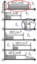
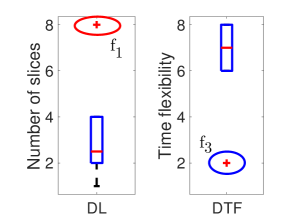
(a)	(b)                 (c)

Figure 3. DL and DTF example, profile size and time flexibility box plots

1:function Initialize($F$)

2:   $\mathit{tft}\leftarrow$LowerFenceTimeFlexibility($F$)

3:   $\mathit{PF}\leftarrow$FOsWithTimeFlexibilityAtLeast$\mathit{tft}$($F,\mathit{tft}$)

4:   $f_{ini}\leftarrow$SelectTheMostFlexibleFOAmongLongest($\mathit{PF}$)

5:   return $\mathit{PF}\setminus f_{ini},F\setminus\mathit{PF},f_{ini},\mathit{tft}$

Algorithm 4 Initialization phase - Dynamic Time Flexibility

Processing phase. In the processing phase, HMAMA examines all the potential binary aggregations between $f_{ini}$ and the FOs in $\mathit{PF}$ defined in the initialization phase. The FOs are examined in descending order according to their time flexibility. FOs with high time flexibility have more potential to participate in an aggregation that fulfills the flexible order requirements because of high number of alignments.

1:function Process($\mathit{PF},\mathit{AF},f_{ini},\mathit{tft},\mathit{ppt},\mathit{spt},e$)

2:   $\mathit{PF}_{tmp}\leftarrow\emptyset$, $\mathit{f}_{a}\leftarrow$ null

3:   for each  $f\in\mathit{PF}$  do

4:     $f_{cand}\leftarrow$ null, $bestCV\leftarrow\infty$

5:     for each alignment $al$ of $\{f_{ini},f\}$  do

6:        $f_{x}\leftarrow$BinaryAggregation($f_{ini},f,al,\mathit{tft},\mathit{ppt}$)

7:        if RMSE($f_{x},\mathit{spt}$)$<$RMSE($f_{ini},\mathit{spt}$) then

8:          if CV($f_{x}$)$<$$bestCV$ then

9:            $bestCV\leftarrow$CV($f_{x}$), $f_{cand}\leftarrow f_{x}$                         

10:     if  $f_{cand}\neq$ null then

11:        $\mathit{PF}_{tmp}\leftarrow\mathit{PF}_{tmp}\cup f$, $f_{ini}\leftarrow f_{cand}$      

12:     if  $\forall s\in P(f_{ini}),spt-e<s.p<spt+e$ then

13:        $f_{a}\leftarrow f_{ini}$

14:        $\mathit{PF}\leftarrow\mathit{PF}\setminus\mathit{PF}_{tmp}$

15:        $\mathit{PF}_{tmp}\leftarrow\emptyset$, $\mathit{spt}\leftarrow\mathit{spt}$$+$$100$         

16:   return $\mathit{PF}$, $\mathit{AF}\cup f_{a}$

Algorithm 5 Processing phase

1:function Examine($\mathit{PF,UF,AF},continue$)

2:   if $\mathit{PF\cup UF}$$=$$\emptyset$ or ($\mathit{|AF|}$$\geq$$5$ and    totalEnergy($\mathit{PF}$$\cup$$\mathit{UF}$)$<$Energy5^thAFO($\mathit{AF}$)) then

3:     $continue\leftarrow false$    

4:   return $\mathit{PF\cup UF}$, $continue$

Algorithm 6 Examination phase

HMAMA examines, through the potential alignments, all the binary aggregations that fulfill the time flexibility $\mathit{tft}$ and the power profile thresholds $\mathit{ppt}$ (Algorithm 5, Lines 3–5). Among the AFOs that reduce the root mean square error (RMSE) between $f_{ini}$ and the slice power threshold $\mathit{spt}$, it chooses the one with the minimum coefficient of variation (CV) (Lines 7–9). By promoting the reduction of RMSE, the produced AFO $f_{cand}$ has a power profile closer to $\mathit{spt}$. In particular, the use of RMSE during aggregation prevents the increase of profile length of the potential AFO and contributes to the production of slices with values closer to $\mathit{spt}$. Consequently, alignments that lead to power profiles that time-wise overlap each other are preferred for aggregation. Moreover, because the slices of an AFO might have power deviations, the second condition of CV (Line 9) is used. A low CV of $f_{cand}$ contributes to the elimination of power profile deviations and to the production of AFOs with slice power amounts closer to each other. For instance, given the FOs in Figure 2 and $\mathit{spt}$ equal to $3$, the RMSE between the slices of AFO $f_{12}$ and $\mathit{spt}$ is equal to $1$ and lower than the RMSE between the longest FO $f_{123}$ and $\mathit{spt}$, which is $1.8$. Similarly, $f_{12}$ and $f_{123}$ have CV equal to $0$ and $0.4$, respectively, with $f_{12}$ having no power fluctuations. Thus, the reduction of RMSE and CV lead to AFOs that fulfill the flexible order energy requirements.

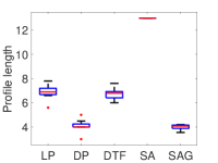
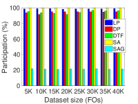
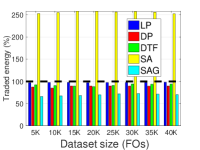
(a) Average time flexibility	(b) Average profile length	(c) Participation in aggregation	(d) Traded energy

Figure 4. Average time flexibility, average profile length, participation of FOs, and traded energy

When an AFO with power amounts around $\mathit{spt}$ is produced, an $e$ kW deviation per slice is permitted (Algorithm 5 Line 12). At that point, an AFO $f_{a}$ that fulfills the flexible order criteria is produced (Line 13). The FOs that participate in aggregation are temporally stored (Line 11) and when an AFO $f_{a}$ is produced, they are removed from $\mathit{PF}$ (Line 14). Then, $\mathit{spt}$ is increased by 100 (Line 15) so that AFOs with larger energy are produced during the following aggregation. As a result, the processing phase produces an AFO that captures large amounts of energy and fulfills the time flexibility and power amount requirements of a flexible order. When all the FOs in $\mathit{PF}$ are processed, HMAMA returns both $\mathit{PF}$ and the output set $\mathit{AF}$ with the aggregated FO $f_{a}$ (Line 16).

Examination phase. During the examination phase, HMAMA first examines if there are any FOs in either $\mathit{PF}$ or $\mathit{UF}$ to further continue aggregation (Algorithm 6 Line 2). In case, the total energy of the remaining FOs is larger than the $5$th in descending size energy AFO, HMAMA continues using the remaining FOs (Line 4). Otherwise, HMAMA does not continue the execution (Line 3). As a result, the algorithm ensures that the remaining FOs cannot produce an AFO with energy greater than one of the $5$ produced AFOs. Since the $5$ AFOs with the most energy will be transformed into flexible orders, the algorithm terminates (Algorithm 1 Line 9).

5. Experimental Evaluation

5.1. Experimental setup

We consider a BRP managing a portfolio of EVs represented by FOs. The BRP utilizes our proposed aggregation algorithms to produce AFOs that respect the flexible order requirements. The BRP transforms the $5$ AFOs which capture the highest amount of energy into flexible orders and trades them in Elspot. In order to examine the scalability of our proposed algorithms, we create $8$ differently-sized FO datasets, from $5$K to $40$K FOs (multiples of $5$K), with characteristics based on the probability distributions suggested in (Vagropoulos et al., 2016). Moreover, we consider that all EVs use the charging option described in Section 2.1 and need to be fully charged. Thus, the initial SOC of all EVs is within [$20$%, $85$%], while they must be charged up to $90$%. Details about the characteristics of the datasets are in Table 1.

We compare our techniques with two baseline aggregation techniques (Siksnys et al., 2015). We use Start-Alignment (SA) aggregation, see Section 3.1 and Start-Alignment Grouping (SAG) aggregation. SAG groups together FOs that have both the same earliest start charging time and the same time flexibility and then applies SA on each group. As a result, it produces one AFO per group. We evaluate our techniques in terms of output size (#AFOs), participation of FOs in aggregation, percentage of energy traded in the market, running time, and both time flexibility and profile length of AFOs.

5.2. Market-based aggregation results

Output size. SA always produces one AFO whereas SAG produces more than $100$ AFOs in all cases. Both LP and DP produce less than or equal to $5$ AFOs in all cases. DTF produces more than $5$ AFOs in $75$% of the cases as the energy threshold is activated in a later step compared to the other techniques due to the division of the processed set.

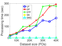
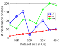
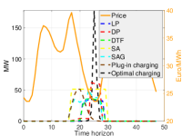
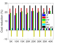
(a) Processing time	(b) # of initialization phases	(c) Charging time vs pricing	(d) Cost reduction

Figure 5. Processing time, number of initialization phases, charging times and pricing for 40K FOs dataset, and cost reduction for all datasets

Time flexibility and profile length. Regarding the baseline techniques, SA produces long AFOs with very low time flexibility as it aggregates all FOs into one. On the contrary, SAG produces short and time flexible AFOs due to the grouping phase it applies, see Figure 4a, b. LP uses as initial FO ($f_{\mathit{ini}}$) the longest FO of the dataset. Usually, such an FO has low time flexibility and so do the produced AFOs. Due to the long profile of $f_{\mathit{ini}}$, LP might utilize all the time flexibility of the remaining FOs to produce an AFO that reduces the distance to the power profile threshold ($\mathit{ppt}$). Consequently, LP produces long AFOs with very low time flexibility, see Figure 4a, b. The AFOs produced by DP are more flexible than the ones from LP since DP applies a dynamic profile size approach and excludes from aggregation very long FOs. As a result, FOs with similar profiles are aggregated together and less time flexibility is required to find a proper alignment that minimizes the distance to $\mathit{ppt}$. Consequently, AFOs with less slices compared to LP are produced, see Figure 4b. Finally, DTF produces the most flexible AFOs among our proposed techniques. We see in Figure 4a that the average time flexibility of the produced AFOs is greater than $4$ in all datasets. DTF achieves it by utilizing the time flexibility threshold. However, DTF produces long AFOs, similar to LP, because it also selects as $f_{\mathit{ini}}$ the longest AFO of the processed set, see Figure 4b.

	Distr.	Mean	St. dev	Min	Max
Battery capacity (kWh)	UD$*$	$23$	4	16	30
Arrival time	TGD$*$	$19$$:$$00$	2h	$16$$:$$00$	$1$$:$$00$
Departure time	TGD$*$	$7$$:$$00$	2h	$5$$:$$00$	$12$$:$$00$
Initial Battery SOE (%)	TGD$*$	75	$25$	$20$	$85$

$*$ UD: uniform distribution, TGD: truncated Gaussian distribution

Table 1. EV data probability distribution

Participation and traded energy. In order to quantify the participation of FOs in aggregation, we take into account only the FOs that participate in the aggregation of the $5$ (or less) largest in energy AFOs, i.e., the AFOs that are transformed into flexible orders. Similarly, we compute the traded energy by taking into account only the energy captured by the AFOs that are transformed into flexible orders.

SA aggregates all FOs into one AFO and thus participation in aggregation is $100$%, see Figure 4c. The slices of the AFO have very high power differences and since a flexible order requires a flat power profile, the power of the highest slice is considered for the whole profile of the AFO. As a result, on average, $2.5$ times the energy captured by that AFO is traded, see Figure 4d where $100$% is the energy needed for all the FOs. On the contrary, SAG produces too many AFOs and since only the $5$ largest are traded, we see a very low participation percentage and the lowest percentage of traded energy among the techniques ($69.7$% on average). In general, the longest AFOs capture more energy as they have more slices and more FOs participate in their aggregation. Thus, LP, which produces the longest AFOs, obtains both the highest participation percentage ($98.6$%) and traded energy percentage ($97.5$%) in all the cases among our proposed techniques, see in Figure 4c, d. DTF follows with an average participation value of $94.4\%$ and $91.7\%$ percentage of traded energy. DP has the lowest percentage in both participation and traded energy, $94.2$% and $88.8$% on average respectively. The reason is that DP excludes very long FOs, which usually capture large energy, from aggregation.

Processing time. Both SA and SAG are fast techniques with processing times below one second as they examine a very small solution space and do not consider the market requirements. LP is the fastest among all our proposed techniques since it efficiently activates the energy threshold, see Figure 5a. The processing time of DP follows a close to linear growth rate. DTF has an increasing trend for processing time, but it shows similar processing times for datasets with different sizes, e.g., for datasets with $30$K and $35$K FOs. The reason is that the processing time is highly driven by the number of initialization phases. The size of the dataset might increase, but the new added FOs might lead to less initialization phases and therefore to less aggregation comparisons. That is why we also notice that both processing time and number of initialization phases follow similar patterns. Whenever the number of initialization phases is increased compared to the previous dataset, processing time also increases. For instance, we see in Figure 5b that when the size of the dataset is increased from $15$K to $20$K for both LP and DTF, the number of initialization phases is reduced. As a result, the processing time is similar for both the datasets and slightly increases for the $25$K. Eventually, when the size of the dataset is further increased, it becomes more difficult for DTF to fulfill the market requirements and thus both the initialization phases and the processing time are highly increased.

5.3. Financial evaluation

Since the overall goal of a BRP is to trade the AFOs in the market using flexible orders, we financially evaluate our aggregation techniques. We compare the cost of buying the energy needed to charge the EVs based on plug-in time (traditional approach) with the cost of charging the EVs by utilizing flexible orders. Moreover, in order to compare our techniques with the optimal solution, we consider a non-realizable in practice scenario where each FO directly participates in the market without aggregation and each EV is charged when the charging cost is minimized.

Due to the fact that flexibility appears during the night (Jin et al., 2013), we consider a $48$ hours trading period with a repetition of the $24$h Elspot average prices of $2017$ (Nor, 2017), see price curve in Figure 5c. In the same figure, we illustrate the time and the energy amount used to charge the $40$K dataset based on our techniques, the two baseline techniques, the plug-in times of the EVs, and the optimal charging. We see that the charging of the EVs based on the plug-in time occurs when the prices are still high and it does not take advantage of the price drop that occurs in the night of the first $24$ hours.

SA and SAG produce AFOs that do not fulfill the market requirements. As a result, more energy than needed has to be traded in the market. In particular, SA trades $1.52$ times more energy than needed to charge the EVs. Thus, the surplus energy is traded in the regulation market and it results in losses for the BRP, see negative cost reduction in Figure 5d. Regarding SAG, the produced AFOs capture a low percentage of the energy needed and they also require extra energy to be traded in order to fulfill the market requirements. Consequently, the cost reduction due to the flexible orders trading is eliminated by the losses from the surplus energy trading. As a result, we see only $1.1$% cost reduction on average when SAG is applied. On the contrary, the optimal charging option charges all the EVs when the price has the lowest value. That is why we see a spike in the graph reaching $180$MW after the $24$^th hour.

Our proposed aggregation techniques also take advantage of the lowest prices. LP produces long AFOs which expand over many hours and have low time flexibility. That is why we see in Figure 5c that part of the charging occurs when the prices are high. DTF produces AFOs that are also long, but they are more flexible than the AFOs produced by LP. Therefore, EVs are charged when prices are a bit lower and DTF achieves a higher cost reduction, Figure 5d. Finally, DP produces short and flexible AFOs. As a result, it takes advantage of the lowest prices occurring only for a few hours, see Figure 5c.

When the energy for the $40$K FOs dataset is purchased based on the plug-in times of the EVs, it costs 8,612 euros. On the contrary, when LP, with the highest participation, is applied on the $40$K dataset, 39,584 FOs participate in aggregation, see first bar ($98.96\%$) in Figure 4c. The 39,584 FOs produce $5$ AFOs which are further transformed into flexible orders. The cost of purchasing the energy needed for the $5$ AFOs is computed based on the flexible orders trading and it is 6,670 euros, see Figure 5c. The price also includes the cost ($0.46$ euro) of the imbalances ($62$kW) of the flexible orders, see Section 2.2. The energy needed for the remaining $416$ (40,000$-$39,584) FOs is bought based on their plug-in time and it is $117$ euros. Thus, the overall energy bought to charge $40$K EVs, when LP is used, costs 6,670$+$126$=$6,796 euros. Therefore, LP achieves a $21$% cost reduction in energy purchase, see LP bar for $40$K dataset in Figure 5d.

We see in Figure 5d that DP achieves on average a 24.4% cost reduction. DTF follows with 20.2% and LP with 19.1% average cost reduction. The cost reduction based on the optimal solution is 27.4% on average. Thus, LP, DTF, and DP achieve $69.8$%, $73.7$%, and $88.9$% of the optimal cost reduction, respectively. Notably, the cost reduction that DP achieves only for the FOs that participate in aggregation is on average $98.3$% of the optimal one.

In Figure 6, we illustrate the cost reduction that DP achieves during $2017$. We consider $364$ trading periods of $48$ hours. The first trading period includes both the $1$^st and the $2$^nd day of $2017$. The second trading period includes the $2$^nd and the $3$^rd day of $2017$ and so on. The average cost reduction is $28$% and, interestingly, we notice at the end of the year a cost reduction of more than $800$%. The reason is that for several consecutive days, Elspot prices were negative early in the morning and even reached $-$$50$ euros/MWh on the $24$^th of December at $2$$:$$0$$0$.

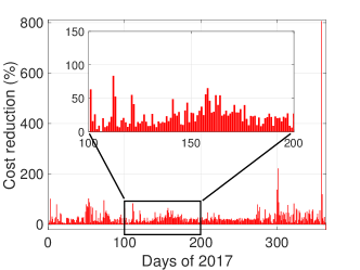
Figure 6. Yearly cost reduction based on DP

Uncertainty on FOs forecast. The driving behavior can usually be forecasted with very high precision and accuracy. However, there might be cases where the anticipated flexible load is smaller because the EVs are not plugged-in as anticipated. Thus, we considered an uncertainty scenario for the $40$K FOs set according to which a percentage of the FOs that participated in aggregation do not need the purchased energy after the flexible orders derived from DP are placed. As a result, BRP has to sell back the exceeded purchased amount of energy for a lower price (regulating price). The difference between the initial cost of purchasing the energy via flexible orders and the cost of the exceeded energy is considered as losses for the BRP. Moreover, BRP has to distribute (assuming no profit) the purchased energy and thus the cost to less costumers (EV owners) compared to the initial estimation. We see in Figure 7, that the price paid by the EV owners based on plug-in time is fixed. On the other hand, the price for the energy purchased via flexible orders increases as the percentage of the EVs that do not participate in aggregation increases. The reason is that the cost is higher due to the imbalances and at the same time less consumers use the purchased energy. We see in Figure 7 that the cost for the consumers via flexible orders is greater than the plug-in charging cost when more than $23$% of the EVs where imprecisely forecasted.

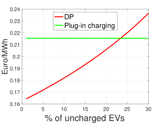
Figure 7. Energy price paid by consumers

Summary: By applying our proposed techniques on the aforementioned $365$ trading periods, DP achieves the highest cost reduction in $66$% of the periods and DTF achieves the highest cost reduction in the remaining $34$% of the periods. The reason is that the financial impact of the techniques is highly correlated with the pricing curve of the trading period. Thus, in cases where the price drops for only few hours close to the plug-in charging time, DP is the most suitable technique. On the other hand, when the price drops for longer periods but much later than the plug-in charging time, DTF achieves a higher reduction than DP.

6. Conclusion and Future work

This paper investigates the market-based aggregation problem using the FO model to capture flexible charging loads of EVs. It proposes $3$ market-based FO aggregation techniques that efficiently aggregate loads from thousand of EVs taking into account real market requirements. Consequently, the techniques produce aggregated FOs that can be transformed into flexible orders and be traded in the energy market. The paper financially evaluates the proposed techniques based on real electricity prices and shows that a $27$% cost reduction on energy purchase can be achieved via flexible orders.

In our future work, we will enrich our techniques considering pricing forecast models and uncertainty in patterns of driving behavior. Furthermore, we will investigate more variations of the proposed algorithm and we prove the theoretical lower bounds for the their complexity. Moreover, we will examine a price-maker market scenario and different market strategies for the BRPs.

- (1)
- mir (2012) 2012. The MIRABEL project. http://www.mirabel-project.eu. (2012).
- tot (2015) 2015. The TotalFlex project. http://www.totalflex.dk. (2015).
- Nor (2017) 2017. Nord pool market. http://www.nordpoolspot.com. (2017).
- Albano et al. (2015) Michele Albano, Luis Lino Ferreira, Luís Miguel Pinho, and Abdel Rahman Alkhawaja. 2015. Message-oriented middleware for smart grids. Computer Standards & Interfaces 38 (2015).
- Baringo and Amaro (2017) L. Baringo and R. S. Amaro. 2017. A stochastic robust optimization approach for the bidding strategy of an electric vehicle aggregator. Electric Power Systems Research 146 (2017).
- Bessa and Matos (2012) R. J. Bessa and M. A. Matos. 2012. Forecasting issues for managing a portfolio of electric vehicles under a smart grid paradigm. In ISGT Europe. https://doi.org/10.1109/ISGTEurope.2012.6465724
- Bessa et al. (2012) R. J. Bessa, M. A. Matos, F. J. Soares, and J. A. P. Lopes. 2012. Optimized Bidding of a EV Aggregation Agent in the Electricity Market. IEEE Trans. on Smart Grid 3 (2012).
- Biegel et al. (2014) B. Biegel, L. H.and J. Stoustrup, P. Andersen, and S. Harbo. 2014. Value of flexible consumption in the electricity markets. Energy 66 (2014).
- Boehm et al. (2012) Matthias Boehm, Lars Dannecker, Andreas Doms, Erik Dovgan, Bogdan Filipič, Ulrike Fischer, Wolfgang Lehner, Torben Bach Pedersen, Yoann Pitarch, Laurynas Šikšnys, and Tea Tušar. 2012. Data Management in the MIRABEL Smart Grid System. In Proceedings of the 2012 Joint EDBT/ICDT Workshops (EDBT-ICDT ’12). 95–102.
- Cao et al. (2012) Y. Cao, S. Tang, C. Li, P. Zhang, Y. Tan, Z. Zhang, and J. Li. 2012. An Optimized EV Charging Model Considering TOU Price and SOC Curve. IEEE Trans. on Smart Grid 3 (2012).
- de Cerio Mendaza et al. (2016) I. Diaz de Cerio Mendaza, I. G. Szczesny, J. R. Pillai, and B. Bak-Jensen. 2016. Demand Response Control in Low Voltage Grids for Technical and Commercial Aggregation Services. IEEE Trans. on Smart Grid 7 (2016). https://doi.org/10.1109/TSG.2015.2465837
- Graham (1994) Ronald L Graham. 1994. Concrete mathematics: a foundation for computer science. Pearson Education India.
- Hu et al. (2016) J. Hu, H. Morais, T. Sousa, and M. Lind. 2016. Electric vehicle fleet management in smart grids: A review of services, optimization and control aspects. Renewable and Sustainable Energy Reviews 56 (2016).
- Jin et al. (2013) C. Jin, J. Tang, and P. Ghosh. 2013. Optimizing Electric Vehicle Charging With Energy Storage in the Electricity Market. IEEE Trans. on Smart Grid 4 (2013).
- Kristoffersen et al. (2011) T. K. Kristoffersen, K. Capion, and P. Meibom. 2011. Optimal charging of electric drive vehicles in a market environment. Applied Energy 88 (2011).
- Liu et al. (2017) Z. Liu, Q. Wu, S. Huang, L. Wang, M. Shahidehpour, and Y. Xue. 2017. Optimal Day-ahead Charging Scheduling of Electric Vehicles through an Aggregative Game Model. IEEE Trans. on Smart Grid PP (2017). https://doi.org/10.1109/TSG.2017.2682340
- Marra et al. (2012) F. Marra, G. Y. Yang, C. Træholt, E. Larsen, C. N. Rasmussen, and S. You. 2012. Demand profile study of battery electric vehicle under different charging options. In Power and Energy Society General Meeting, IEEE.
- Michael Frigge (1989) Boris Iglewicz Michael Frigge, David C. Hoaglin. 1989. Some Implementations of the Boxplot. The American Statistician 43 (1989).
- Mittelmann (2016) H. Mittelmann. 2016. Benchmark of commercial LP solvers. http://plato.asu.edu/ftp/lpcom.html. (2016).
- Neupane et al. (2017) Bijay Neupane, Laurynas Šikšnys, and Torben Bach Pedersen. 2017. Generation and Evaluation of Flex-Offers from Flexible Electrical Devices. In Proceedings of the Eighth International Conference on Future Energy Systems (e-Energy ’17). ACM, New York, NY, USA, 143–156. https://doi.org/10.1145/3077839.3077850
- Sarker et al. (2016) M. R. Sarker, Y. Dvorkin, and M. A. Ortega-Vazquez. 2016. Optimal Participation of an Electric Vehicle Aggregator in Day-Ahead Energy and Reserve Markets. IEEE Trans. on Power Systems 31 (2016).
- Siksnys et al. (2015) L. Siksnys, E. Valsomatzis, K. Hose, and T. B. Pedersen. 2015. Aggregating and Disaggregating Flexibility Objects. IEEE Trans. on Knowledge and Data Engineering 27 (2015).
- Vagropoulos et al. (2016) S. I. Vagropoulos, D. K. Kyriazidis, and A. G. Bakirtzis. 2016. Real-Time Charging Management Framework for Electric Vehicle Aggregators in a Market Environment. IEEE Trans. on Smart Grid 7 (2016).
- Valsomatzis et al. (2015) Emmanouil Valsomatzis, Katja Hose, Torben Bach Pedersen, and Laurynas Siksnys. 2015. Measuring and Comparing Energy Flexibilities. In CEUR Workshop Proceedings, Vol. 1330. 78–85.
- Valsomatzis et al. (2016) E. Valsomatzis, T. B. Pedersen, A. Abelló, and K. Hose. 2016. Aggregating energy flexibilities under constraints. In Smart Grid Communications (SmartGridComm), 2016 IEEE International Conference on. IEEE. 484–490.
- Vandael et al. (2015) S. Vandael, B. Claessens, D. Ernst, T. Holvoet, and G. Deconinck. 2015. Reinforcement Learning of Heuristic EV Fleet Charging in a Day-Ahead Electricity Market. IEEE Trans. on Smart Grid 6 (July 2015). https://doi.org/10.1109/TSG.2015.2393059
- Vaya and Andersson (2015) M. Gonzalez Vaya and G. Andersson. 2015. Optimal Bidding Strategy of a Plug-In Electric Vehicle Aggregator in Day-Ahead Electricity Markets Under Uncertainty. IEEE Trans. on Power Systems 30 (2015).
- Šikšnys and Pedersen (2016) Laurynas Šikšnys and Torben Bach Pedersen. 2016. Dependency-based FlexOffers: Scalable Management of Flexible Loads with Dependencies. In Proceedings of the Seventh International Conference on Future Energy Systems (e-Energy ’16).
- Weron (2006) Rafal Weron. 2006. Modeling and Forecasting Electricity Loads and Prices. John Wiley & Sons Ltd. https://doi.org/10.1002/9781118673362.ch1
- Yang et al. (2014) L. Yang, J. Zhang, and H. V. Poor. 2014. Risk-Aware Day-Ahead Scheduling and Real-time Dispatch for Electric Vehicle Charging. IEEE Trans. on Smart Grid 5 (2014).
- Zhao et al. (2017) J. Zhao, C. Wan, Z. Xu, and J. Wang. 2017. Risk-Based Day-Ahead Scheduling of Electric Vehicle Aggregator Using Information Gap Decision Theory. IEEE Trans. on Smart Grid PP (2017). https://doi.org/10.1109/TSG.2015.2494371