Anomalous effects of velocity rescaling algorithms: the flying ice cube effect revisited

Abstract

The flying ice cube effect is a molecular dynamics simulation artifact in which the use of velocity rescaling thermostats sometimes causes the violation of the equipartition theorem, affecting both structural and dynamic properties. The reason for this artifact and the conditions under which it occurs have not been fully understood. Since the flying ice cube effect was first demonstrated, a new velocity rescaling algorithm (the CSVR thermostat) has been developed and become popular without its effects on the equipartition theorem being truly known. Meanwhile, use of the simple velocity rescaling and Berendsen thermostat algorithms has not abated but has actually continued to grow. Here, we have calculated the partitioning of the kinetic energy between translational, rotational, and vibrational modes in simulations of diatomic molecules to explicitly determine whether the equipartition theorem is violated under different thermostats and while rescaling velocities to different kinetic energy distributions. We have found that the underlying cause of the flying ice cube effect is a violation of balance leading to systematic redistributions of kinetic energy under simple velocity rescaling and the Berendsen thermostat. When velocities are instead rescaled to the canonical ensemble’s kinetic energy distribution, as is done with the CSVR thermostat, the equipartition theorem is not violated, and we show that the CSVR thermostat satisfies detailed balance. The critical necessity for molecular dynamics practitioners to abandon the use of popular yet incorrect velocity rescaling algorithms is underscored with an example demonstrating that the main result of a highly-cited study is entirely due to artifacts resulting from the study’s use of the Berendsen thermostat.

Berkeley] Department of Chemical and Biomolecular Engineering, University of California, Berkeley, Berkeley, CA 94720, USA EPFL] Institut des Sciences et Ingénierie Chimiques (ISIC), Valais, École Polytechnique Fédérale de Lausanne (EPFL), Rue de l’Industrie 17, CH-1951 Sion, Switzerland Berkeley] Department of Chemical and Biomolecular Engineering, University of California, Berkeley, Berkeley, CA 94720, USA [EPFL] Institut des Sciences et Ingénierie Chimiques (ISIC), Valais, École Polytechnique Fédérale de Lausanne (EPFL), Rue de l’Industrie 17, CH-1951 Sion, Switzerland

1 Introduction

By integrating the classical Newtonian equations of motion, molecular dynamics (MD) simulations naturally sample the microcanonical (NVE) ensemble due to conservation laws.^{1, 2} For comparison with experiment, it is often desirable to sample constant-temperature ensembles such as the canonical (NVT) or isothermal-isobaric (NPT) ensembles. In analogy with experiment, these ensembles could be generated by sampling a subspace of a much larger microcanonical system that serves as a heat bath, but such an approach is usually too computationally-expensive to implement in practice. Instead, various thermostatting algorithms are typically applied to change the Hamiltonian dynamics in a manner such that the intended ensemble is sampled. Many such algorithms have been proposed, and some of the more well-known choices include:

• Simple velocity rescaling, pioneered by Woodcock ³ for thermal equilibration, rescales the velocities of all particles at the end of each timestep (it can also be conducted with a less frequent time rescaling period) by a factor $\lambda$ to achieve a target instantaneous temperature: $\lambda=\left(\frac{{\lx@glossaries@gls@link{main}{Ktar}{\leavevmode K_{\text{target}}}}}{K}\right)^{\frac{1}{2}}$ with $\lx@glossaries@gls@link{main}{Ktar}{\leavevmode K_{\text{target}}}=\frac{1}{2}N_{\text{DOF}}k_{\text{B}}T_{\text{target}}$, where $N_{\text{DOF}}$ is the number of degrees of freedom in the system.

• The Gaussian thermostat supplements Newton’s second law with a force intended to keep the kinetic energy constant:^{4, 5, 6} $\mathbf{\dot{p}}_{i}=-\nabla U_{i}-\alpha\mathbf{p}_{i}$, where $\alpha$ is a Lagrange multiplier determined using Gauss’ principle of least constraint to be $\alpha=\left.\left(\sum_{i=1}^{N}\mathbf{F}_{i}\cdot\mathbf{p}_{i}/m_{i}\right)\middle/\left(\sum_{i=1}^{N}\mathbf{p}_{i}^{2}/m_{i}\right)\right.$.

• Langevin dynamics supplements Newton’s second law with terms describing Brownian motion:⁷ $\mathbf{\dot{p}}_{i}=-\nabla U_{i}-\gamma\mathbf{p}_{i}+\mathbf{\eta}$, where $\gamma$ represents a frictional dissipative force and $\mathbf{\eta}(t,T,\gamma,m_{i})$ is a stochastic term representing random collisions.

• The Berendsen thermostat takes the Langevin equation, removes the stochastic term, and modifies the frictional dissipative force to yield similar temperature time dependence as with the stochastic term present:⁸ $\mathbf{\dot{p}}_{i}=-\nabla U_{i}-\gamma\mathbf{p}_{i}\left(\frac{\lx@glossaries@gls@link{main}{Ktar}{\leavevmode K_{\text{target}}}}{K}-1\right)$, where $\lx@glossaries@gls@link{main}{Ktar}{\leavevmode K_{\text{target}}}=\frac{1}{2}N_{\text{DOF}}k_{\text{B}}T_{\text{target}}$. In practice, this is implemented as a smoother version of the simple velocity rescaling technique, in which the velocities of all particles are rescaled at the end of each timestep by a factor $\lambda$, with $\lambda=\left[1+\frac{\Delta t}{\tau_{T}}\left(\frac{\lx@glossaries@gls@link{main}{Ktar}{\leavevmode K_{\text{target}}}}{K}-1\right)\right]^{\frac{1}{2}}$. $\tau_{T}$ represents a time damping constant; if it is set equal to the timestep, the Berendsen algorithm recovers simple velocity rescaling, and as the time damping constant approaches infinity, the Berendsen algorithm recovers conventional microcanonical dynamics.

• The canonical sampling through velocity rescaling (CSVR) thermostat is a velocity rescaling algorithm in which the velocities of all particles are rescaled at the end of each timestep by a factor $\lambda$ designed such that the kinetic energy exhibits the distribution of the canonical ensemble.^{9, 10} To this end, $\lambda=\left(\frac{{\lx@glossaries@gls@link{main}{Ktar}{\leavevmode K_{\text{target}}}}}{K}\right)^{\frac{1}{2}}$, where Ktarget is stochastically drawn from the probability density function $P(\lx@glossaries@gls@link{main}{Ktar}{\leavevmode K_{\text{target}}})\propto\lx@glossaries@gls@link{main}{Ktar}{\leavevmode K_{\text{target}}}^{\nicefrac{{N_{\text{DOF}}}}{{2}}-1}e^{-\beta\lx@glossaries@gls@link{main}{Ktar}{\leavevmode K_{\text{target}}}}$. This algorithm can be adjusted to yield a smoother evolution in a similar manner as the Berendsen algorithm smoothes simple velocity rescaling.⁹

• The Nosé-Hoover thermostat extends the classical Lagrangian to include the additional coordinate $s$ and its time-derivative:^{11, 12} $\mathcal{L}=s^{2}\sum_{i=1}^{N}\frac{\mathbf{p}_{i}^{2}}{2m_{i}}-U+\frac{1}{2}Q\dot{s}^{2}-k_{\text{B}}T_{\text{target}}L\ln s$, where $Q$ is the effective “mass” associated with $s$ and $L$ is set by the number of degrees of freedom. A single Nosé-Hoover thermostat may be used, or chains of thermostats may be implemented to improve ergodicity and to take into account additional conservation laws.¹³

There exist numerous additional thermostats (e.g., the Andersen thermostat¹⁴), and small changes can be made to the listed thermostats, such as implementing the originally global Nosé-Hoover thermostat in a local “massive” manner by pairing a separate Nosé-Hoover thermostat to each degree of freedom.¹⁵ The reader is referred to a non-comprehensive list of reviews and textbooks for additional information.^{16, 17, 1, 18}

Simple velocity rescaling and the Gaussian thermostat aim to sample the isokinetic ensemble (NVK). However, they are often presented as equivalent to the canonical ensemble with respect to position-dependent equilibrium properties, with justification for this based on the argument that the configurational part of the isokinetic ensemble’s partition function is exactly equal to that of the canonical ensemble’s.^{19, 20, 5, 21, 22} Meanwhile, the Berendsen thermostat does not correspond to a known ensemble but is rather supposed to sample a configurational phase space intermediate to the canonical and microcanonical ensembles.^{8, 23, 24}

In the 1990s, it was found that the simple velocity rescaling and Berendsen thermostat algorithms introduce an artifact:^{25, 26} the “flying ice cube effect,” as coined by Harvey et al. ²⁶, describes a violation of the equipartition theorem observed when using these algorithms in which kinetic energy drains from high-frequency modes such as bond stretching into low-frequency modes such as center of mass (COM) translation. This was shown to affect systems’ structural, thermodynamic, and dynamic properties.²⁶ As it can be proven that the equipartition theorem holds in the canonical ensemble, microcanonical ensemble, and isokinetic ensemble (see Appendix),^{27, 28, 29, 30, 31} a simulation exhibiting the flying ice cube effect is not ergodically sampling any of these ensembles, neither in configurational phase space nor in momentum phase space.

Nonetheless, simple velocity rescaling and the Berendsen thermostat continue to be commonly used,^{17, 32} with Cooke and Schmidler ³² stating, “By far the most commonly used algorithm for constant temperature MD of biomolecules is the Berendsen heat bath, due to its ease of implementation and availability in standard software packages.” Use of the Berendsen thermostat can be approximated by tracking citations of its canonical reference,⁸ which have continued to grow over time (Fig. 1).

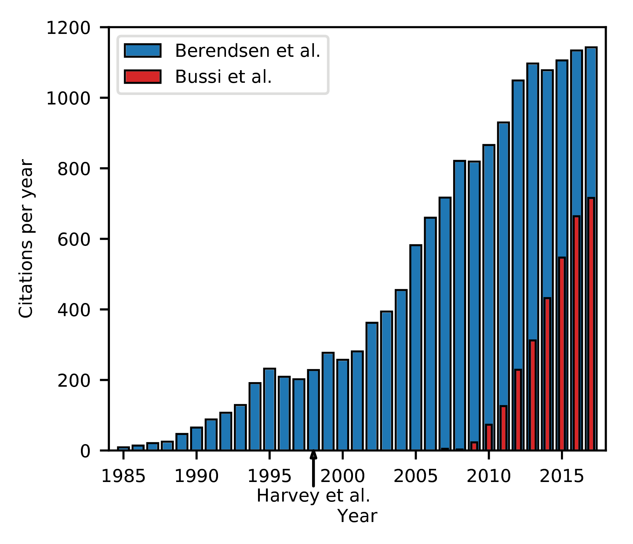
Figure 1: Citations of Berendsen et al. ⁸ and Bussi et al. ⁹ over time. Data provided by Web of Science, extracted on 2018-05-04.

Some technical aspects of the flying ice cube effect are as of yet still unclear. Since Harvey et al. ²⁶, there has been continued discussion about whether the flying ice cube effect may occur with other thermostats.^{33, 34} The CSVR thermostat rescales velocities to yield the canonical ensemble’s distribution of kinetic energies, similar to how simple velocity scaling yields the isokinetic ensemble’s distribution of kinetic energies and the Berendsen thermostat yields a kinetic energy distribution intermediate to the two ensembles. If all velocity rescaling algorithms always lead to the flying ice cube effect, then it may be suspected that the same flying ice cube artifact occurs when using the CSVR thermostat,³⁵ which would be worrisome because the CSVR thermostat has been quickly adopted into widespread use (Fig. 1). In addition, since the Gaussian thermostat has been shown to be similar to simple velocity rescaling,³⁶ it may be suspected that the Gaussian thermostat exhibits the artifact as well. Given the wide-spread use of these algorithms in MD simulations, more understanding is warranted, and we will show that neither the CSVR thermostat nor the Gaussian thermostat bring about the flying ice cube effect.

In the present work we refer to the flying ice cube effect as the term was originally used to describe the violation of the equipartition theorem as caused by velocity rescaling procedures.²⁶ Other MD simulation methods that fail to conserve energy in the microcanonical ensemble can also bring about equipartition theorem violations.³³ These methods include approximate treatment of long-range electrostatic interactions, certain multiple timestep algorithms, constraining molecular geometries with too loose of a tolerance, not updating neighbor lists frequently enough, and using too large of a timestep.^{37, 33, 38} In some cases these issues are also referred to as flying ice cube effects,^{39, 40, 41} but these are not related to the artifact with which we are concerned.

In this work, we have revisited the simple model system of united-atom diatomic ethane molecules that Harvey et al. ²⁶ first used to illustrate the flying ice cube effect. By explicitly calculating the partitioning of kinetic energies between translational, rotational, and vibrational degrees of freedom, we are able to determine which thermostats and conditions lead to the violation of equipartition, as well as the manner and degree to which they do so. We go on to rationalize these findings by illustrating how simple velocity rescaling violates balance, while the CSVR thermostat satisfies detailed balance. We end by illustrating some severe errors that are directly caused by these subtleties related to thermostatting.

2 Simulation Details

Diatomic ethane molecule simulations were conducted with the open-source LAMMPS code.⁴² LAMMPS input scripts are available. We used the 2016-11-17 release of LAMMPS to conduct our simulations. The Gaussian thermostat was not implemented in LAMMPS, so we wrote an extension that integrates the equations of motion given by Minary et al. ²¹. This extension was later incorporated into the LAMMPS code and made publicly available starting with the 2017-01-06 update as part of the “fix nvk” command.

Except where stated otherwise, the simulations consisted of cubic simulation boxes with periodic boundary conditions (PBC), setup by placing the ethane molecules on a simple cubic lattice, equilibrated with a Langevin thermostat for at least $50\text{\,}\mathrm{ns}$, switched to the target thermostat for at least a further $50\text{\,}\mathrm{ns}$ of equilibration, and finally ran with the target thermostat for at least $50\text{\,}\mathrm{ns}$ of production. We verified that all simulations were conducted for sufficient time periods for the energies to equilibrate and be well sampled. The velocities of the particles in microcanonical simulations were rescaled once after Langevin equilibration such that the total energy was equal to the average total energy seen in the Langevin simulation. For the simulations in which the COM linear momentum was fixed to zero (stated in the figure captions), the system’s linear momentum was zeroed every timestep, followed by a rescaling of velocities to maintain the same total kinetic energy as before the zeroing had occurred to prevent energy leakage. The equations of motion were integrated with a standard Velocity Verlet algorithm using half-step velocity calculations. The timestep used was $0.5\text{\,}\mathrm{fs}$, which was found to give adequate energy conservation in the microcanonical ensemble.

Thermostat parameters were as follows, except where stated otherwise. Simple velocity rescaling was done every timestep. The Nosé-Hoover chain consisted of three thermostats. The Berendsen, Nosé-Hoover, and CSVR thermostats were used with time damping constants ($\tau_{T}$) of $100\text{\,}\mathrm{fs}$, and the Nosé-Hoover thermostat used effective thermostat masses of $Q_{1}=N_{\text{DOF}}k_{\text{B}}T{\tau_{T}}^{2}$ and $Q_{i>1}=k_{\text{B}}T{\tau_{T}}^{2}$.¹³ When doing simulations in the microcanonical ensemble, the total energy was set such that a simulation temperature equal to the canonical ensemble simulations’ target temperature was achieved. The target simulation temperature was set to $350\text{\,}\mathrm{K}$, well above the critical temperature of ethane.⁴⁴

Kinetic energies of each diatomic molecule were partitioned into translational, rotational, and vibrational kinetic energies, as shown in the Appendix. In all figures that plot kinetic energies, the error bars shown represent $\pm 1$ standard error of the mean. This was calculated by dividing the data from the production timesteps into $20$ consecutive blocks, averaging the data for each block, and computing the standard error over the $20$ data values.¹ Error bars are not shown when they would be smaller than the symbols or the line widths.

Bonded parameters for the united-atom ethane molecule were taken from Harvey et al. ²⁶ (harmonic bond potential $U(r)=k(r-r_{0})^{2}$ with $r_{0}=$$1.54\text{\,}\mathrm{\SIUnitSymbolAngstrom}$ and $k=$$240\text{\,}\mathrm{kcal}\text{\,}{\mathrm{mol}}^{-1}\text{\,}{\mathrm{\SIUnitSymbolAngstrom}}^{-2}$) and non-bonded parameters were taken from Martin and Siepmann ⁴⁴ (Lennard-Jones potential with $\epsilon=$$0.195\text{\,}\mathrm{kcal}\text{\,}{\mathrm{mol}}^{-1}$, $\sigma=$$3.75\text{\,}\mathrm{\SIUnitSymbolAngstrom}$, truncated and shifted at $14\text{\,}\mathrm{\SIUnitSymbolAngstrom}$, and no charges).

Details on the simulations of benzene in MOF-5 can be found in the Appendix.

3 Results and Discussion

3.1 Examining equipartition under different thermostats

It is instructive to reconsider the simple case previously examined by Harvey et al. ²⁶: that of a single ethane molecule moving in one-dimensional space along its bond axis. In the microcanonical ensemble under perfect energy conservation, the translational kinetic energy will remain constant at its set initial energy and the vibrational kinetic energy will oscillate. In the canonical ensemble, equipartition states that the translational and vibrational degree of freedom should each have an average kinetic energy of $\frac{1}{2}k_{\text{B}}T$. As expected, the Langevin thermostat satisfies the equipartition theorem (see Fig. 2). In agreement with the work of Harvey et al. ²⁶, we find that simple velocity rescaling and the Berendsen thermostat bring about a violation of equipartition in the kinetic degrees of freedom, with all kinetic energy flowing to translational motion, in the plainest illustration of the flying ice cube effect. We find that the CSVR thermostat correctly partitions the energies.

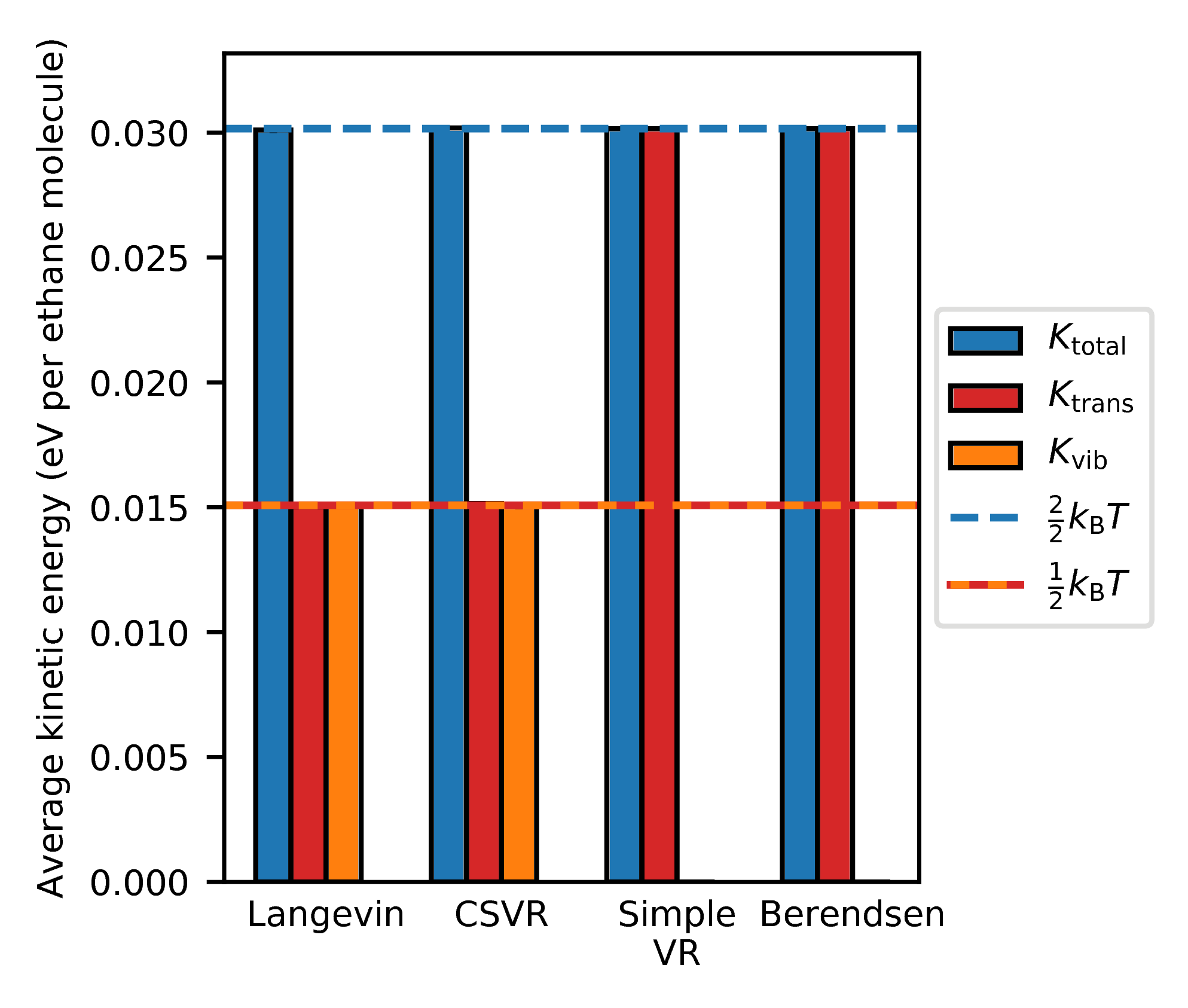
Figure 2: Partitioning of the kinetic energies obtained from one-dimensional MD simulations of a single ethane molecule using various thermostats. Both atoms were given a starting velocity of $100\text{\,}\mathrm{m}\text{\,}{\mathrm{s}}^{-1}$ along the same direction as the bond vector. For the thermostats shown, the same energy partitionings were observed regardless of initial bond length and initial COM momentum. The microcanonical, Nosé-Hoover thermostat, and Gaussian thermostat results are not shown here since we found that the energy partitionings are dependent on the initial conditions, indicative of these thermostats’ well-known lacks of ergodicity that are more manifest for small systems.^{1, 5, 45, 36, 13, 46, 47, 17}

We next consider the more complex case of a large number of ethane molecules interacting in three dimensions with anharmonic Lennard-Jones potentials. Each diatomic ethane molecule now has three translational modes, two rotational modes, and one vibrational modes, so the equipartition theorem states that these modes’ kinetic energies should be equal to $\frac{3}{2}k_{\text{B}}T$, $\frac{2}{2}k_{\text{B}}T$, and $\frac{1}{2}k_{\text{B}}T$ respectively, with a correction of $\frac{3}{2}k_{\text{B}}T/N_{\rm{molecs}}$ to the translational kinetic energy in cases where the COM momentum is constrained. In Fig. 3, we show that the Langevin, Nosé-Hoover, CSVR, and Gaussian thermostats all exhibit correctly equipartitioned energies, as does the microcanonical ensemble. As in the case of the single ethane molecule in one dimension, the simple velocity rescaling and Berendsen thermostat algorithms lead to a violation of equipartition, with translational and rotational modes having too much kinetic energy and vibrational modes having too little.

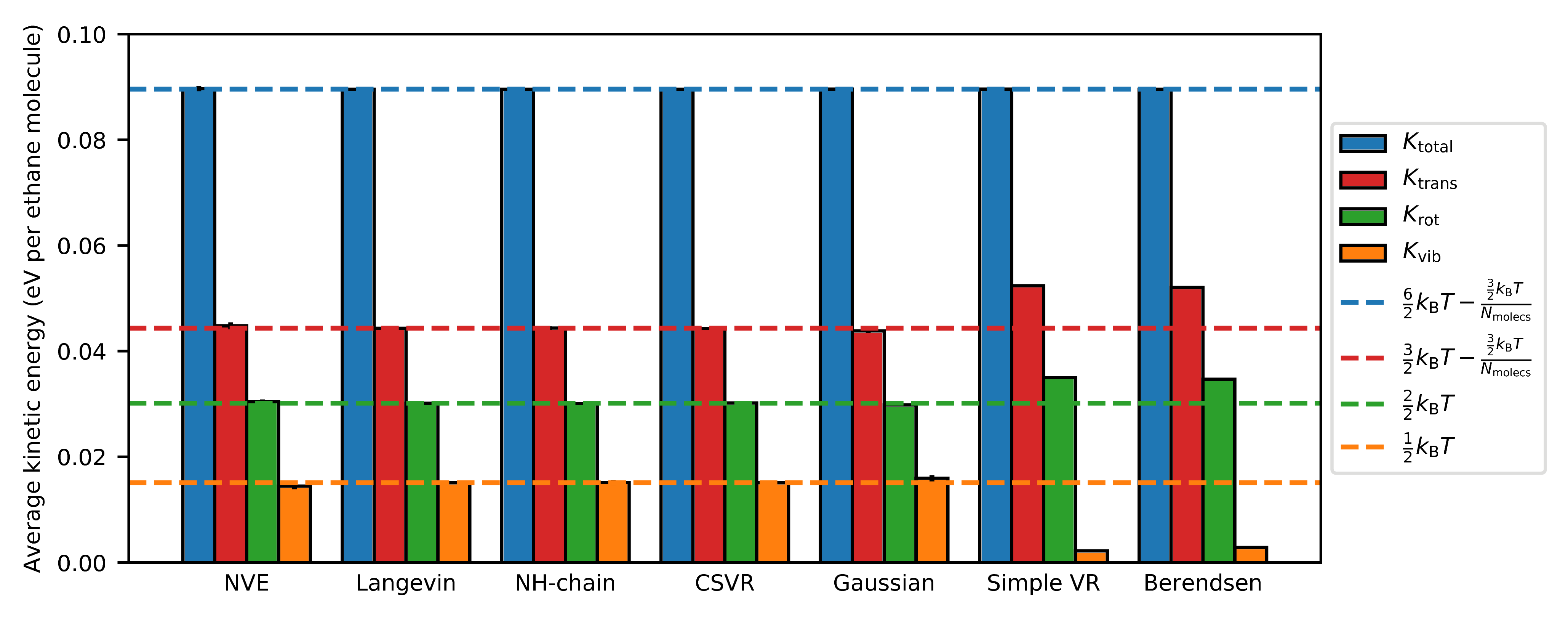
Figure 3: Partitioning of the kinetic energies obtained from MD simulations of 50 ethane molecules in a $30\text{\,}\mathrm{\SIUnitSymbolAngstrom}$ cubic simulation box using various thermostats. In all simulations shown, the COM momentum was fixed to zero.

3.2 Equivalence of simple velocity rescaling and the Gaussian thermostat

Since the thermostatting under simple velocity rescaling does not take place within the equations of motion, this ad hoc temperature control algorithm was initially difficult to investigate theoretically, and its validity was considered questionable.^{5, 6} The algorithm’s use was justified on the basis of empirical arguments, such as that simple velocity rescaling and the Gaussian thermostat give similar static and dynamic properties for the Lennard-Jones fluid.¹⁹ It was eventually proven that simple velocity rescaling is analytically equivalent to the Gaussian thermostat within an error of $\mathcal{O}\left(\text{timestep}\right)$ when the velocity rescaling time period is set equal to the timestep,³⁶ which gave support for the legitimacy of using simple velocity rescaling to sample the isokinetic ensemble.

However, we have shown that the Gaussian thermostat exhibits correct energy equipartitioning while simple velocity rescaling does not. We prove in the Appendix that the isokinetic ensemble should satisfy the equipartition theorem. Thus, it is clear that simple velocity rescaling does not actually sample the isokinetic ensemble.

The equivalence of simple velocity rescaling and the Gaussian thermostat under small timesteps leads to the expectation that the flying ice cube effect will gradually disappear under simple velocity rescaling as the timestep is decreased. We demonstrate confirmation of this expectation in Fig. 4. However, Fig. 4 shows that the timestep needs to be reduced by over three orders of magnitude from typical simulation timesteps before the flying ice cube effect is no longer discerned. Of course, such a decreased timestep requires an equivalent three orders of magnitude increase in CPU time; if the timestep between integrations is so small, the forces on the particles should not need to be recalculated every timestep, and so one could envision implementing a multiple-time-step algorithm to mitigate the increase in CPU time. We also note that under the Berendsen thermostat, lowering the timestep does not correct the energy partitioning.

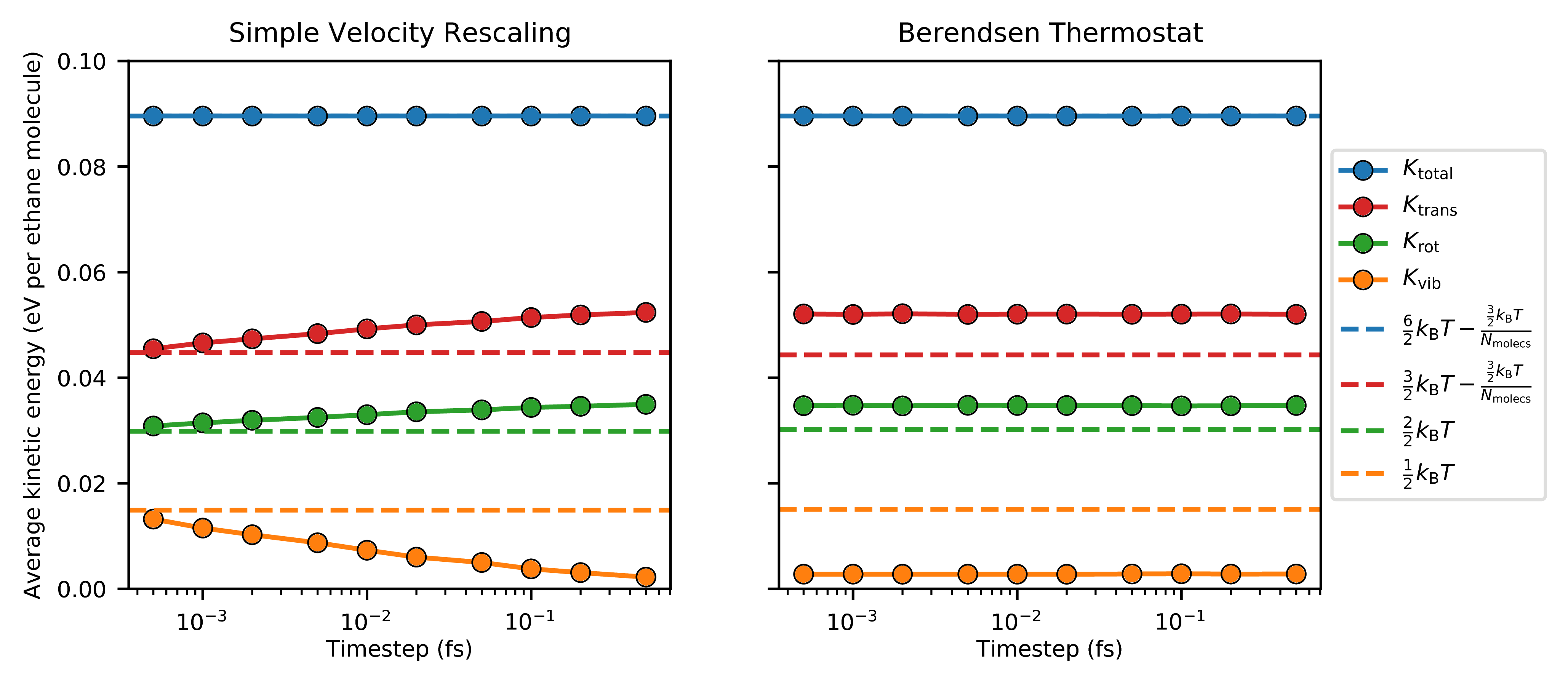
Figure 4: Partitioning of the kinetic energies obtained from MD simulations performed under the same conditions as in Fig. 3 but changing the timestep, using (left) simple velocity rescaling and (right) the Berendsen thermostat with the time damping constant maintained at $100\text{\,}\mathrm{fs}$. Lines are a guide to the eye.

3.3 Violation of balance causes the flying ice cube effect

The mechanism underlying the flying ice cube effect can be elucidated graphically for the first test case we examined, that of a single ethane molecule. In Fig. 5, we show this system’s phase space, putting translational kinetic energy on the $x$-axis and vibrational kinetic energy on the $y$-axis.

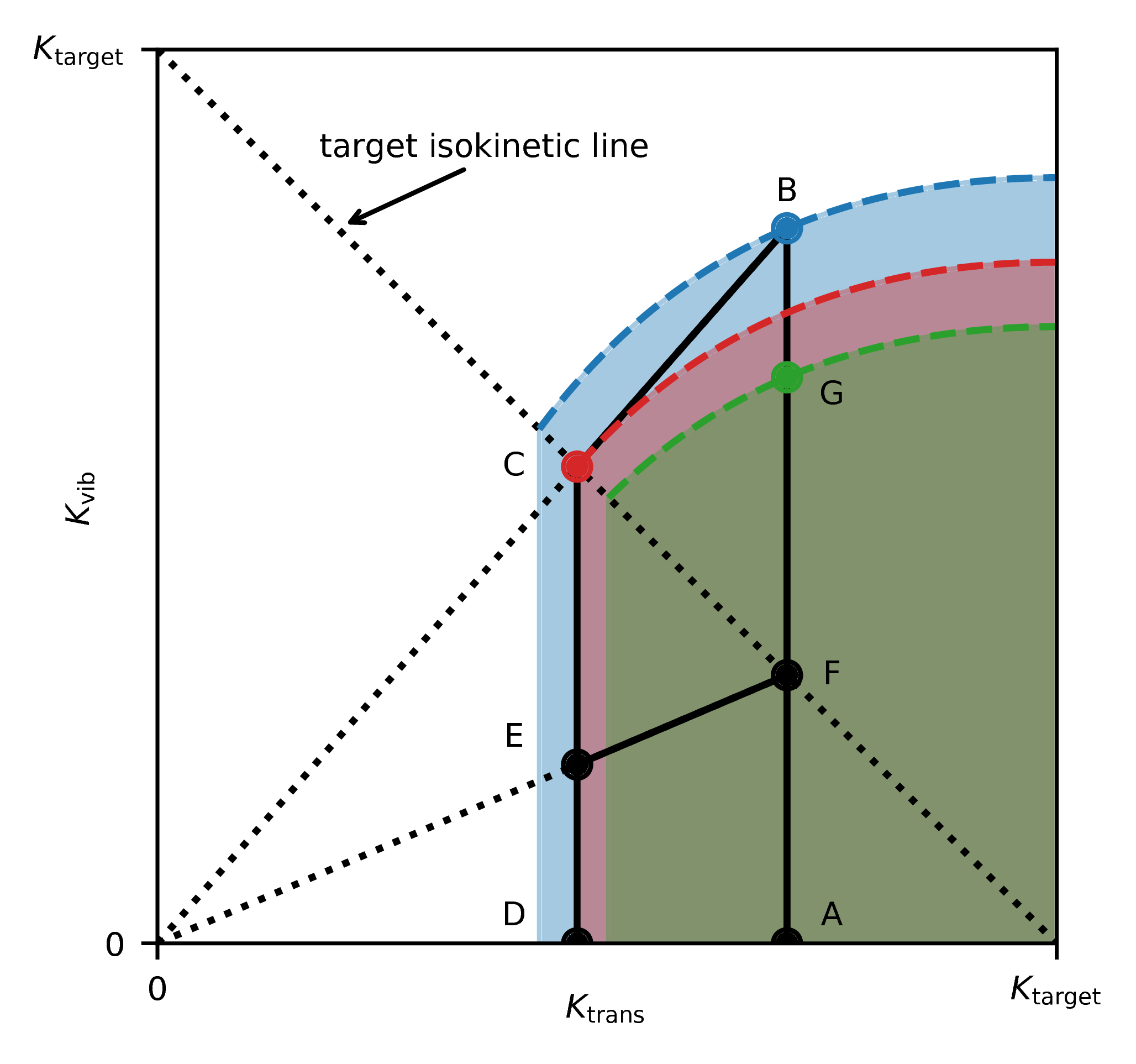
Figure 5: Kinetic phase space of a single ethane molecule moving in one-dimensional space along its bond axis under simple velocity rescaling. $\lx@glossaries@gls@link{main}{Ktar}{\leavevmode K_{\text{target}}}=k_{\text{B}}T_{\text{target}}$, $K_{\rm{trans}}=\frac{1}{2}\left(m_{1}+m_{2}\right)\left(\frac{m_{1}v_{1,x}+m_{2}v_{2,x}}{m_{1}+m_{2}}\right)^{{}^{2}}$, and $K_{\rm{vib}}=\frac{1}{2}\left(\frac{m_{1}m_{2}}{m_{1}+m_{2}}\right)\left(v_{2,x}-v_{1,x}\right)^{2}$. Solid lines show a particular path in phase space between labeled points, referred to in the text. Dotted lines are guides useful to understanding the velocity rescaling moves. Dashed lines show the boundaries of phase space accessible by any sequence of MD and velocity rescalings from lines $\overline{AB}$, $\overline{CD}$, and $\overline{AG}$, with the accessible phase spaces shaded.

During microcanonical MD, the system can only explore phase space on a vertical line between $y=0$ and $y=U_{\rm{max}}$ because a constant total energy and translational kinetic energy is maintained, with energy exchanges only allowed between vibrational kinetic energy and potential energy. Consider a MD simulation initially on such a vertical line in phase space, $\overline{AB}$. Under simple velocity rescaling, if a rescaling move is conducted at point $B$, the system will move to point $C$; this occurs because the translational and vibrational energies are both scaled by the same factor $\lambda^{2}$ such that their sum is equal to the target kinetic energy, moving the system to the intersection of the lines $y=\frac{y_{B}}{x_{B}}x$ and the target isokinetic line ($y=-x+K_{\rm{target}}$). Since points $B$ and $C$ have the same configuration with zero potential energy, MD will now explore line $\overline{CD}$.

Let us examine whether we can reach point $B$ by rescaling from line $\overline{CD}$ back to a line with the same translational energy of line $\overline{AB}$. With a single rescaling, we would need to rescale from point $E$ to point $F$. From point $F$, MD will explore phase space on line $\overline{AG}$, where the lengths of lines $\overline{FG}$ and $\overline{CE}$ are equal, with both representing the stored potential energy of the system prior to the rescaling. Obviously, line $\overline{EF}$ must have a smaller slope than line $\overline{BC}$; accordingly, $y_{G}$ will necessarily be smaller than $y_{B}$. Hence, with a single velocity rescaling, point $B$ cannot be reached. Multiple velocity rescalings from line $\overline{CD}$ allows us to reach a point with greater vibrational kinetic energy than point $G$. However, all phase space reachable by any number of velocity rescalings from line $\overline{CD}$ is bounded by the red dashed line in Fig. 5 (see Appendix for derivation). Continuing to rescale will continue to shrink the volume of accessible phase space, as rescaling from lines $\overline{AB}$ to $\overline{CD}$ to $\overline{AG}$ lowers the boundary from the blue to the red to the green dashed lines; eventually, accessible phase space will be confined only to the point with all kinetic energy in the translational mode.

Notably, the decrease in accessible phase space becomes smaller as velocity rescaling occurs closer to the isokinetic line. In a simulation, this occurs when the timestep between velocity rescalings is reduced. This explains why the flying ice cube effect is reduced under simple velocity rescaling by decreasing the timestep (Fig. 4).

3.3.1 Monte Carlo perspective

We can view the combination of MD and velocity scaling moves as a Monte Carlo simulation. Hence, our previous example shows that simple velocity rescaling violates the condition of balance.^{48, 1}

In contrast, the CSVR thermostat can explicitly be proven to sample the desired distribution by considering the condition of detailed balance. Let us assume that we do a large and random number of MD steps between velocity rescaling moves. We define $A$ as the set of all configurations of the system with a total energy $E_{A}$. The flow of configurations from set $A$ to set $B$ is given by:

$$K\left(A\rightarrow B\right)=$$

$$\quad P\left(E_{A}\right)\sum_{{\bf r}_{1}^{n}}\sum_{{\bf p}_{1}^{n}}\sum_{{\bf r}_{2}^{n}}\sum_{{\bf p}_{2}^{n}}p\left({\bf r}_{1}^{n},{\bf p}_{1}^{n}|E_{A}\right)\delta\left(E\left({\bf r}_{1}^{n},{\bf p}_{1}^{n}\right)-E_{A}\right)\alpha\left({\bf r}_{1}^{n},{\bf p}_{1}^{n}\rightarrow{\bf r}_{2}^{n},{\bf p}_{2}^{n}\right)\delta\left(E\left({\bf r}_{2}^{n},{\bf p}_{2}^{n}\right)-E_{B}\right)$$ (1)

where ${\bf r}_{1}^{n},{\bf p}_{1}^{n}$ is the configuration with position vector ${\bf r}_{1}^{n}$ and momentum vector ${\bf p}_{1}^{n}$, $p\left({\bf r}_{1}^{n},{\bf p}_{1}^{n}|E_{A}\right)$ is the probability to find the configuration ${\bf r}_{1}^{n},{\bf p}_{1}^{n}$ from all configurations with energy $E_{A}$ during MD, and $\alpha\left({\bf r}_{1}^{n},{\bf p}_{1}^{n}\rightarrow{\bf r}_{2}^{n},{\bf p}_{2}^{n}\right)$ is the a priori probability to velocity rescale from configuration ${\bf r}_{1}^{n},{\bf p}_{1}^{n}$ to configuration ${\bf r}_{2}^{n},{\bf p}_{2}^{n}$. Recognizing that velocity rescaling does not alter positions:

$$K\left(A\rightarrow B\right)=P\left(E_{A}\right)\sum_{{\bf r}^{n}}\sum_{{\bf p}_{1}^{n}}\sum_{{\bf p}_{2}^{n}}p\left({\bf r}^{n},{\bf p}_{1}^{n}|E_{A}\right)\delta\left(E\left({\bf r}_{1}^{n},{\bf p}_{1}^{n}\right)-E_{A}\right)\alpha\left({\bf r}^{n},{\bf p}_{1}^{n}\rightarrow{\bf r}^{n},{\bf p}_{2}^{n}\right)\delta\left(E\left({\bf r}^{n},{\bf p}_{2}^{n}\right)-E_{B}\right)$$ (2)

Next, recognizing that velocity rescaling can only give one configuration in momentum space with $E\left({\bf r}^{n},{\bf p}_{2}^{n}\right)=E_{B}$ from starting configuration ${\bf r}^{n},{\bf p}_{1}^{n}$, and that the acceptance probabilities only involve the kinetic energy:

$$K\left(A\rightarrow B\right)=P\left(E_{A}\right)\sum_{{\bf r}^{n}}\sum_{{\bf p}^{n}}p\left({\bf r}^{n},{\bf p}^{n}|E_{A}\right)\delta\left(E\left({\bf r}_{1}^{n},{\bf p}_{1}^{n}\right)-E_{A}\right)\alpha\left(K=E_{A}-U\left({\bf r}^{n}\right)\rightarrow E_{B}-U\left({\bf r}^{n}\right)\right)$$ (3)

where $\alpha\left(K=E_{A}-U\left({\bf r}^{n}\right)\rightarrow E_{B}-U\left({\bf r}^{n}\right)\right)$ is the a priori probability to velocity rescale to the configuration having kinetic energy $K=E_{B}-U\left({\bf r}^{n}\right)$ given we start with a configuration having kinetic energy $K=E_{A}-U\left({\bf r}^{n}\right)$. Then, recognizing that momentum and position are decoupled, i.e., the number of possible states in momentum space only depends on the total kinetic energy but does not depend on the details of the potential energy surface, and each of these possible states in momentum space are equally likely:

$$K\left(A\rightarrow B\right)=P\left(E_{A}\right)\sum_{{\bf r}^{n}}\omega\left(E_{A}-U\left({\bf r}^{n}\right)\right)p\left({\bf r}^{n},{\bf p}^{n}|E_{A}\right)\alpha\left(K=E_{A}-U\left({\bf r}^{n}\right)\rightarrow E_{B}-U\left({\bf r}^{n}\right)\right)$$ (4)

where $\omega\left(K\right)$ is the number of configurations in momentum space for a given kinetic energy $K$ (equivalent to the ideal gas microcanonical partition function). Finally, by making the substitutions $p\left({\bf r}^{n},{\bf p}^{n}|E_{A}\right)=\Omega_{NVE_{A}}^{-1}$ and $P\left(E_{A}\right)=\frac{e^{-\beta E_{A}}\Omega_{NVE_{A}}}{Z_{NVT}}$:

$$K\left(A\rightarrow B\right)=\frac{e^{-\beta E_{A}}}{Z_{NVT}}\sum_{{\bf r}^{n}}\omega\left(E_{A}-U\left({\bf r}^{n}\right)\right)\alpha\left(K=E_{A}-U\left({\bf r}^{n}\right)\rightarrow E_{B}-U\left({\bf r}^{n}\right)\right)$$ (5)

The two flows, $K\left(A\rightarrow B\right)$ and $K\left(B\rightarrow A\right)$, are equal if we impose as condition for the a priori probabilities:

$$\frac{\alpha\left(K=E_{A}-U\left({\bf r}^{n}\right)\rightarrow E_{B}-U\left({\bf r}^{n}\right)\right)}{\alpha\left(K=E_{B}-U\left({\bf r}^{n}\right)\rightarrow E_{A}-U\left({\bf r}^{n}\right)\right)} =\frac{e^{-\beta E_{B}}\omega\left(E_{B}-U\left({\bf r}^{n}\right)\right)}{e^{-\beta E_{A}}\omega\left(E_{A}-U\left({\bf r}^{n}\right)\right)}$$

$$=\frac{e^{-\beta\left(E_{B}-U\left({\bf r}^{n}\right)\right)}\left(E_{B}-U\left({\bf r}^{n}\right)\right)^{\nicefrac{{N_{\text{DOF}}}}{{2}}-1}}{e^{-\beta\left(E_{A}-U\left({\bf r}^{n}\right)\right)}\left(E_{A}-U\left({\bf r}^{n}\right)\right)^{\nicefrac{{N_{\text{DOF}}}}{{2}}-1}}$$ (6)

in which we used the known expression for the ideal gas microcanonical partition function.¹⁸ Eq. 6 is satisfied by the CSVR thermostat, which rescales velocities to the target kinetic energy distribution given by the gamma distribution:

$$P(K)=\frac{e^{-\beta K}K^{\nicefrac{{N_{\text{DOF}}}}{{2}}-1}}{\int_{0}^{\infty}dKK^{\nicefrac{{N_{\text{DOF}}}}{{2}}-1}e^{-\beta K}}=\frac{e^{-\beta K}K^{\nicefrac{{N_{\text{DOF}}}}{{2}}-1}}{\beta^{-\nicefrac{{N_{\text{DOF}}}}{{2}}}\Gamma\left(\nicefrac{{N_{\text{DOF}}}}{{2}}\right)}$$ (7)

Hence, the CSVR thermostat satisfies detailed balance.

3.3.2 Velocity rescaling to other kinetic energy distributions

We have seen that simple velocity rescaling violates balance and brings about the flying ice cube effect, while the CSVR thermostat satisfies detailed balance and does not exhibit the artifact. One key difference between these algorithms is that simple velocity rescaling restricts the rescaling factor ($\lambda$) to be less than one when the system’s instantaneous temperature is greater than the target temperature and greater than one when the instantaneous temperature is less than the target temperature. It is this restriction which allowed us to show graphically that simple velocity rescaling moves decrease accessible phase space. It is instructive to consider the effects of relaxing this restriction while rescaling velocities to a non-canonical kinetic energy distribution. This procedure would not render any areas of phase space inaccessible, but the rescaling would be to a distribution that is not necessarily invariant under Hamiltonian dynamics.^{14, 48}

To change the target kinetic energy distribution, we modified the CSVR thermostat’s value of $N_{\text{DOF}}$ in Eq. 7 from the actual number of degrees of freedom ($N_{\text{DOF},0}$) while simultaneously adjusting $\beta$ from its initial value ($\beta_{0}$) such that $\beta=\beta_{0}\frac{N_{\text{DOF}}}{N_{\text{DOF},0}}$ in order to maintain a constant average kinetic energy. The resulting kinetic energy distributions are shown in the top of Fig. 6 and include distributions that are sharper ($N_{\text{DOF}}>N_{\text{DOF},0}$) and broader ($N_{\text{DOF}}<N_{\text{DOF},0}$) than the canonical distribution. In the limit of $N_{\text{DOF}}\to\infty$, this method closely approximates simple velocity rescaling or the Berendsen thermostat, depending on the time damping constant used.

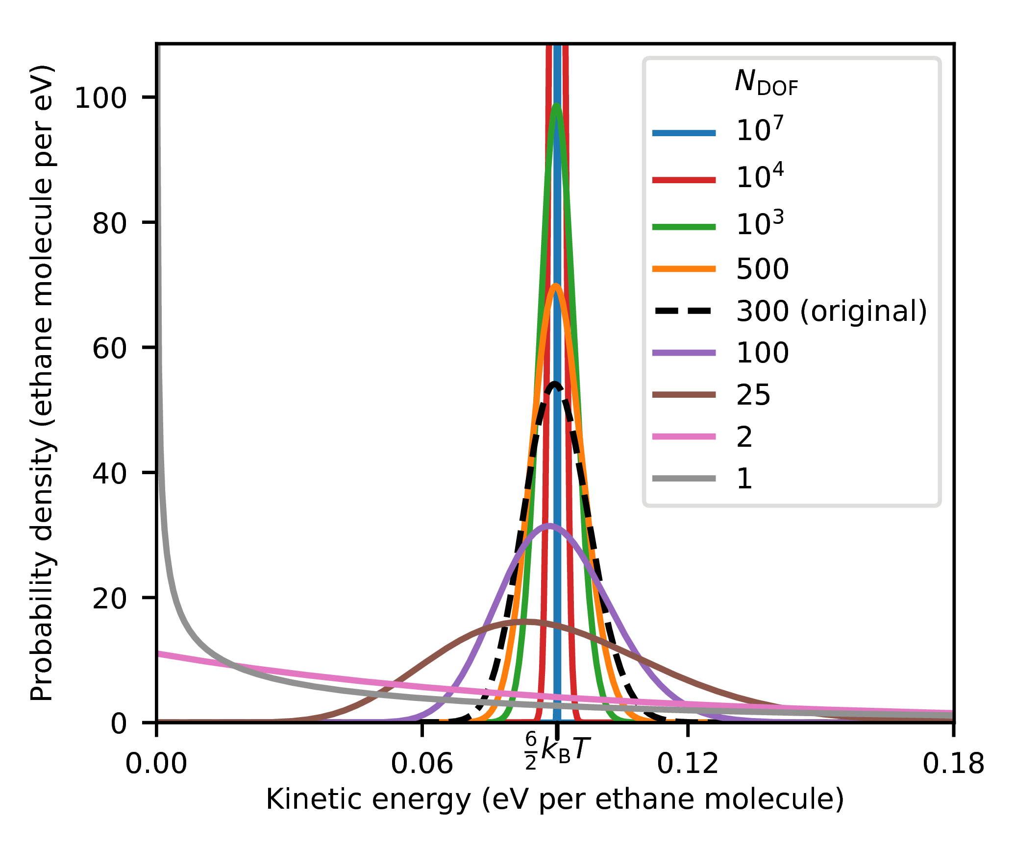
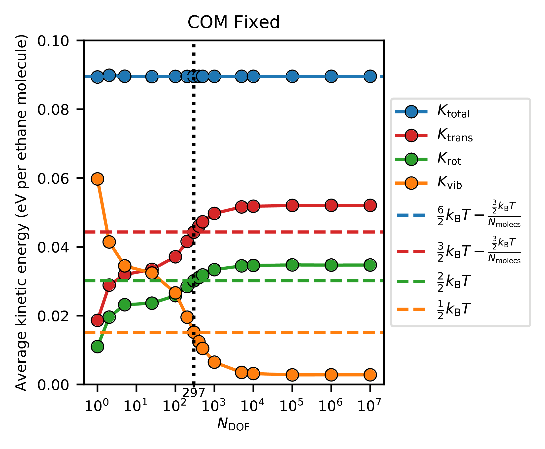
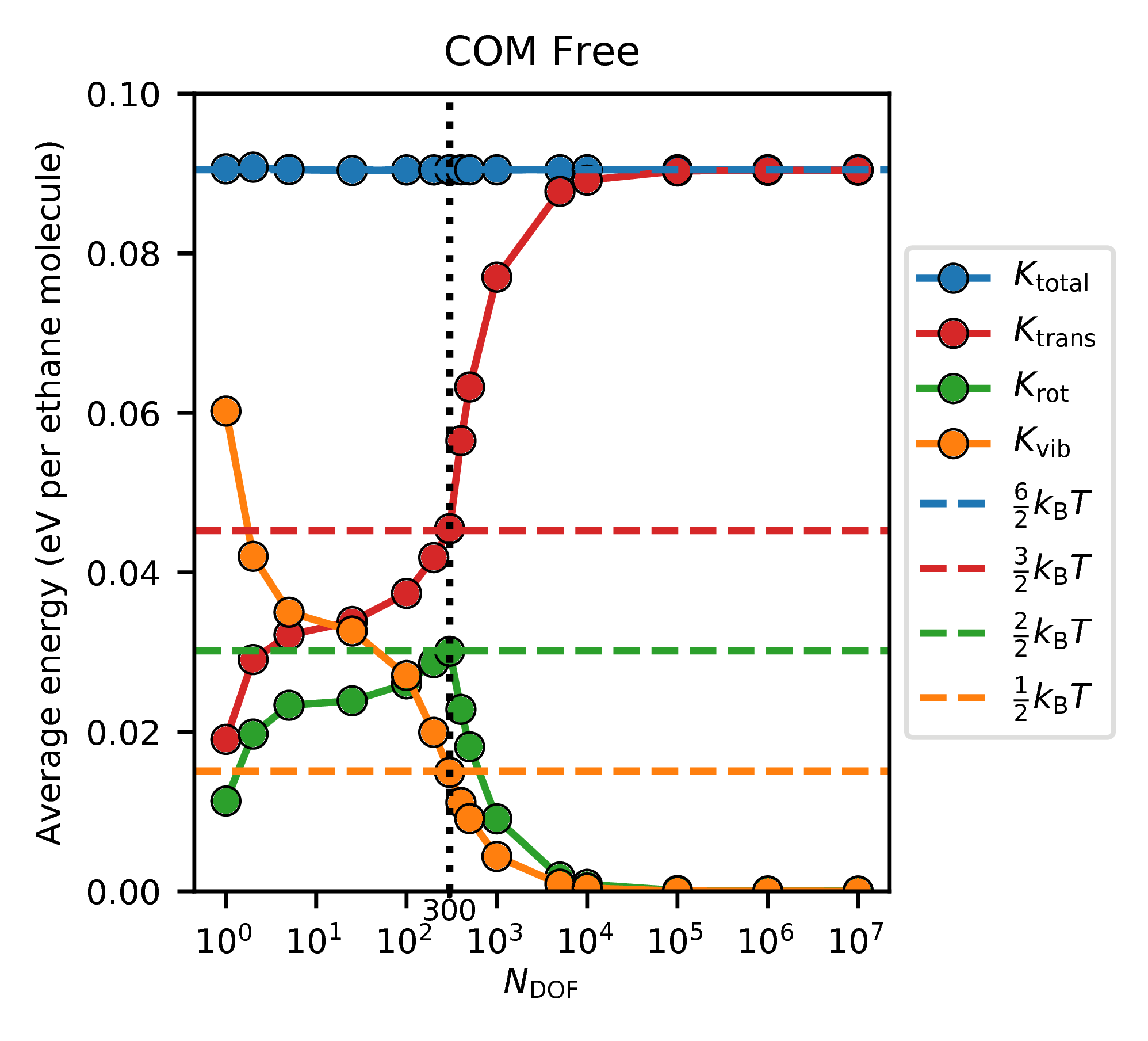
Figure 6: (top) Probability density function of kinetic energies following $P(K)=\frac{e^{-\beta K}K^{\nicefrac{{N_{\text{DOF}}}}{{2}}-1}}{\beta^{-\nicefrac{{N_{\text{DOF}}}}{{2}}}\Gamma\left(\nicefrac{{N_{\text{DOF}}}}{{2}}\right)}$, where $\beta$ is chosen such that the average kinetic energy (temperature) is the same for all choices of $N_{\text{DOF}}$ via $\beta=\beta_{0}\frac{N_{\text{DOF}}}{N_{\text{DOF},0}}$, $N_{\text{DOF},0}=300$, and $\beta_{0}=\left(k_{\text{B}}\times 350\text{ K}\right)^{-1}$. (bottom) Partitioning of the kinetic energies obtained from MD simulations of 50 ethane molecules in a $30\text{\,}\mathrm{\SIUnitSymbolAngstrom}$ cubic simulation box using the CSVR thermostat, modified such that the target distribution of kinetic energies was set to those shown in the top part of the figure for the proper $N_{\text{DOF},0}$ value. (bottom left) Here, the COM momentum was fixed at zero and $N_{\text{DOF},0}$ was set to 297. (bottom right) Here, the COM momentum was not fixed after the Langevin thermostat equilibration, allowing the COM momentum to drift, and $N_{\text{DOF},0}$ was set to 300. Lines are a guide to the eye.

The energy partitionings that resulted from setting these target kinetic energy distributions are shown for simulations in the bottom of Fig. 6. It can be seen that with sharper distributions, the flying ice cube effect is observed, with more kinetic energy partitioned in low-frequency modes and less in high-frequency modes. Interestingly, the opposite effect is observed with broader distributions, with more kinetic energy partitioned in high-frequency modes and less in low-frequency modes. When the COM momentum is not constrained to zero, a more drastic effect is observed, such that rotational kinetic energy decreases both with decreasing $N_{\text{DOF}}$ as energy flows to the higher-frequency vibrational modes and with increasing $N_{\text{DOF}}$ as almost all energy flows to the lower-frequency translational modes. Only at the canonical kinetic energy distribution ($N_{\text{DOF}}=297$ and $N_{\text{DOF}}=300$ for the constrained and not-constrained COM momentum simulations, respectively) is proper equipartitioning observed.

3.4 Conditions affecting the flying ice cube effect’s conspicuousness

Artifacts relating to the flying ice cube effect do not always appear when the simple velocity rescaling or Berendsen thermostat algorithms are used.^{49, 50, 35} Indeed, when the flying ice effect was first found,^{25, 26} fewer alternatives to these thermostatting algorithms were available than at present, e.g., the CSVR thermostat had not yet come into popular use, and so protective measures were recommended to lower the likelihood of the artifact occurring under these faulty thermostats.²⁶ Here, we investigate these recommendations and other conditions which we found affect the conspicuousness of the flying ice cube effect for our system of interacting diatomic ethane molecules.

One recommendation given in Harvey et al. ²⁶ was to lower the thermostat’s coupling strength, either by less frequent rescaling under simple velocity rescaling or by increasing the time damping constant under the Berendsen thermostat. Decreasing the coupling strength allows for the system’s natural dynamics to bring about energy equipartitioning faster than the thermostat can disturb it. In Fig. 7, we show that this recommendation does indeed reduce the violation of equipartition. However, the flying ice cube artifact was not fully resolved until these time parameters were larger than $100\text{\,}\mathrm{ps}$, a value much greater than the $0.5\text{\,}\mathrm{ps}$ time damping constant above which Berendsen et al. ⁸ showed that energy fluctuations under the Berendsen thermostat are similar to energy fluctuations in the microcanonical ensemble and thus concluded that the thermostat has little influence on the dynamics. This discrepancy may be partially explained by the use of the rigid SPC water model⁵¹ to evaluate the Berendsen thermostat in Berendsen et al. ⁸, as a rigid molecule lacks the high-frequency vibrational modes that lead most directly to the flying ice cube effect. Meanwhile, we found that energy equipartitioning held under the CSVR thermostat regardless of the value of the time damping constant. At the weakest coupling strengths shown in Fig. 7, it can be seen that the desired temperature was not well established in these $100\text{\,}\mathrm{ns}$ simulations.

Varying the coupling strength does not come without its risks. Fig. 7 shows an anomalous data point when simple velocity rescaling is performed every $500\text{\,}\mathrm{fs}$. Further investigation allowed us to characterize this anomaly as a resonance effect associated with bond vibration. The characteristic period of the CH3-CH3 harmonic bond is $38.4\text{\,}\mathrm{fs}$. When the time rescaling period is set close to an integer multiple of half this characteristic period, large amplitude bond vibrations occur, becoming stronger when the time rescaling period more exactly matches the multiple. These resonance effects become weaker as the multiple grows, which explains why the vibrational energy at the time rescaling period of $1000\text{\,}\mathrm{fs}$ is greater than at $2000\text{\,}\mathrm{fs}$. We observed resonance effects when rescaling close to other multiples of half the bond’s characteristic period that we also tested. We will shortly show that altering the coupling strength can bring about resonance effects under the Berendsen thermostat as well.

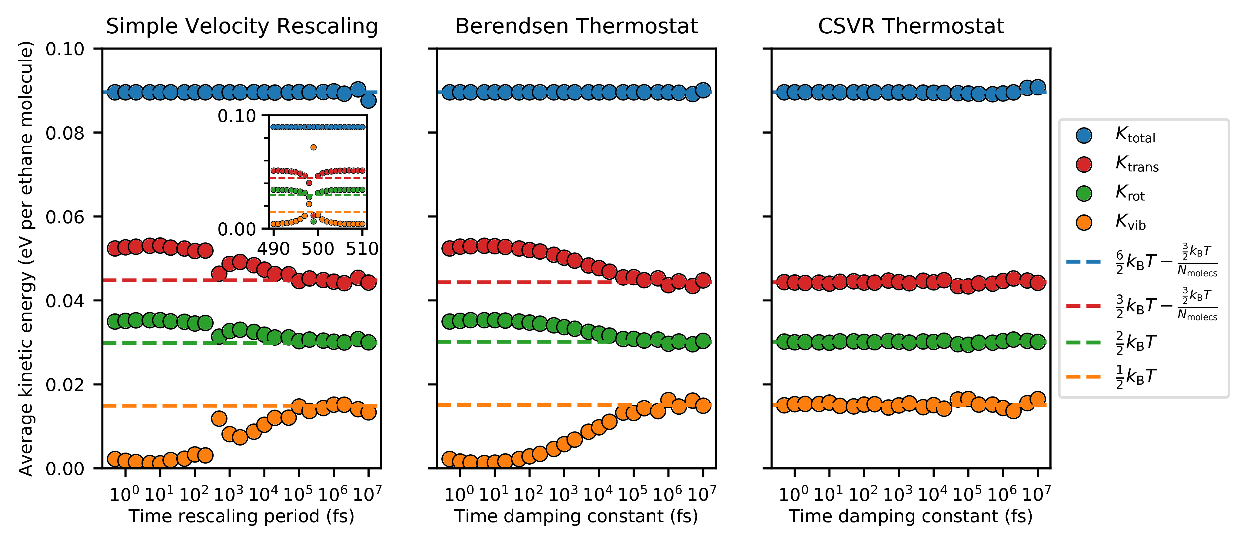
Figure 7: Partitioning of the kinetic energies obtained from MD simulations performed under the same conditions as in Fig. 3, but changing (left) the time rescaling period for simple velocity rescaling, (middle) the time damping constant for the Berendsen thermostat, and (right) the time damping constant for the CSVR thermostat, all three with the timestep maintained at $0.5\text{\,}\mathrm{fs}$. The inset shown in the simple velocity rescaling graph shows additional data near the time rescaling period of $500\text{\,}\mathrm{fs}$, at which point a resonance artifact associated with the CH3-CH3 bond’s characteristic vibrational frequency can be observed.

Another precautionary measure recommended in Harvey et al. ²⁶ was to periodically zero the COM momentum, as it represents the lowest-frequency degree of freedom into which most kinetic energy flows. The Newtonian equations of motion preserve COM momentum, but numeric errors cause this preservation to be inexact. Constraint of the COM momentum to zero is oftentimes used to safeguard against these numeric errors: a safeguard we used throughput this paper except where stated. In Fig. 8, we show that releasing this constraint does indeed significantly worsen the flying ice cube effect, though equipartition is violated both with and without the constraint. We further explored the effects of allowing the COM momentum to vary by replacing the PBC with reflecting walls, which we found gets rid of the flying ice cube effect completely, with no violation of the equipartition theorem. In both of these cases, COM momentum is not conserved, but with opposite results observed (though in the former case, COM momentum can build-up, while in the latter case, it cannot), We hypothesize that reflecting walls void the flying ice cube effect because the additional collisions with the walls give additional opportunities for energy to be transferred between kinetic modes, which acts more quickly than the Berendsen thermostat works to incorrectly partition the energy. To test this hypothesis, we made the walls softer so that a smaller redistribution of intramolecular kinetic energy would take place upon collision. Instead of reflecting walls, we used wall-particle interactions with a softer 9-3 Lennard-Jones potential,⁵² $U(r)=\epsilon\left[\frac{2}{15}\left(\frac{\sigma}{r}\right)^{9}-\left(\frac{\sigma}{r}\right)^{3}\right]$ with arbitrary $\epsilon$ and $\sigma$ values of $0.195\text{\,}\mathrm{kcal}\text{\,}{\mathrm{mol}}^{-1}$ and $3.75\text{\,}\mathrm{\SIUnitSymbolAngstrom}$, respectively, and a shifted cutoff of $14\text{\,}\mathrm{\SIUnitSymbolAngstrom}$. We found that with this softer wall, energy equipartitioning holds less well than with the harder wall, giving some support to our hypothesis. We note further that the presence of the reflecting wall did not significantly change the distribution of total kinetic energies, i.e., the wall did not bring about equipartition indirectly through bringing about a more proper kinetic energy distribution.

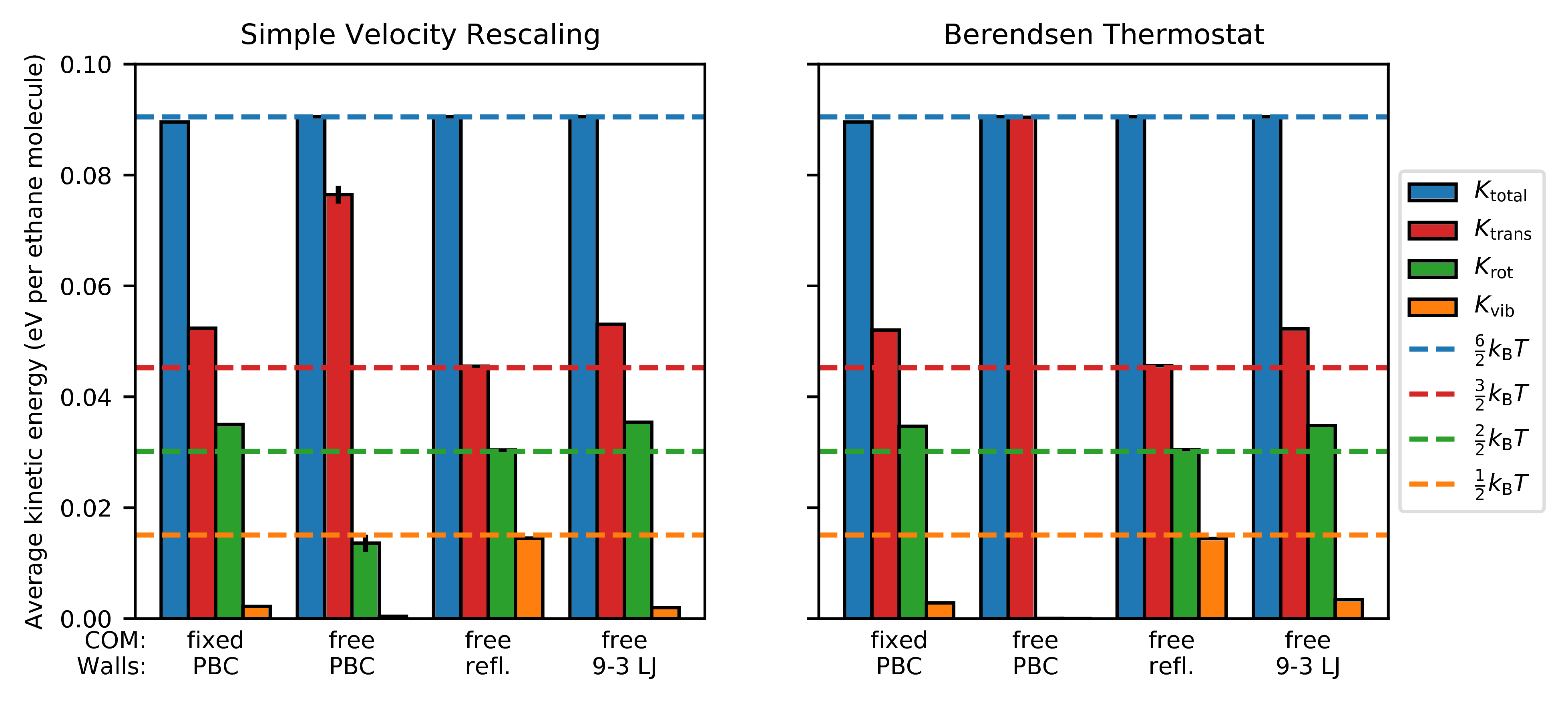
Figure 8: Partitioning of the kinetic energies obtained from MD simulations of 50 ethane molecules in a $30\text{\,}\mathrm{\SIUnitSymbolAngstrom}$ cubic simulation box under different conditions using (left) simple velocity rescaling and (right) the Berendsen thermostat. In each, the first simulation from left is the same simulation as shown in Fig. 3 and provides a basis for comparison. The second simulation shows the effects of letting the COM momentum drift (COM: free) as opposed to fixing it to zero (COM: fixed). The third and fourth simulations show the effects of hard (PBC: reflecting) and soft (PBC: 9-3 Lennard-Jones) wall boundaries, respectively, as opposed to PBC (Walls: PBC). Note that the dashed lines meant as a guide to the eye do not include the COM momentum constraint correction of $\frac{\frac{3}{2}k_{\text{B}}T}{N_{\rm{molecs}}}$ that is reflected in the first simulation.

Finally, we found that increasing the size of the simulation box reduces the flying ice cube effect, as can be seen in Fig. 9. As with decreasing the timestep (Fig. 4), here too we find that simple velocity rescaling recovers equipartition more easily than the Berendsen thermostat. We conjecture that this finite size effect occurs because the canonical ensemble’s distribution of kinetic energy becomes more sharply peaked with increasing number of particles, i.e., the ratio of the standard deviation to the mean of the canonical kinetic energy distribution (the gamma distribution given in Eq. 7) scales as $\mathcal{O}\left(\frac{1}{\sqrt{N_{\text{DOF}}}}\right)$ at constant temperature. Thus, as the number of particles increases, simple velocity rescaling and the Berendsen thermostat become more similar to the CSVR thermostat.

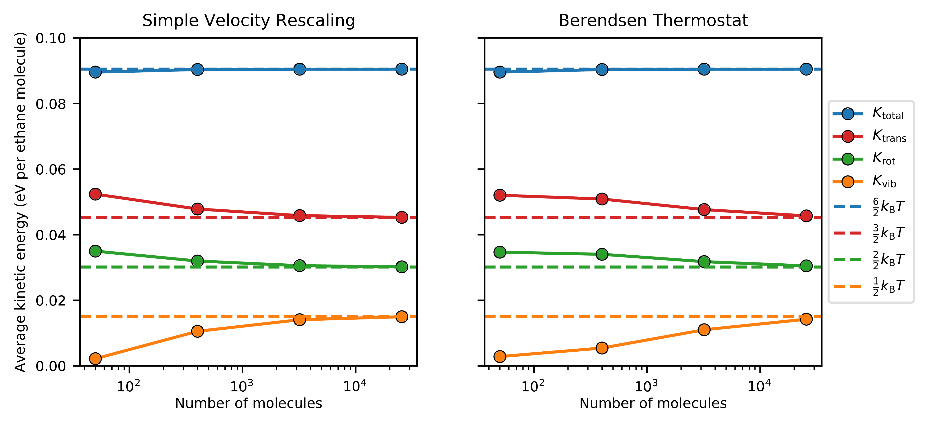
Figure 9: Partitioning of the kinetic energies obtained from MD simulations performed under the same conditions as in Fig. 3 but changing the number of ethane molecules, using (left) simple velocity rescaling and (right) the Berendsen thermostat. The simulation with 50 ethane molecules took place in a $30\text{\,}\mathrm{\SIUnitSymbolAngstrom}$ cubic simulation box, and the other simulations had their simulation boxes enlarged to maintain the same density. Note that the dashed lines meant as a guide to the eye do not include the COM momentum constraint correction of $\frac{\frac{3}{2}k_{\text{B}}T}{N_{\rm{molecs}}}$, which is responsible for the slight deviation of the total kinetic energy from $\frac{6}{2}k_{\text{B}}T$ that is more evident for the simulations with less molecules.

3.5 Sampling configurational degrees of freedom

So far, we have exclusively used kinetic degrees of freedom to show that the simple velocity rescaling and Berendsen thermostat algorithms cause the violation of equipartition. These methods are sometimes used only to sample configurational degrees of freedom, justified on the grounds that the isokinetic ensemble samples the same configurational phase space as the canonical ensemble.^{19, 20, 5, 21, 22} Since we have proven that the violation of equipartition is incommensurate with sampling the isokinetic ensemble, it follows that this justification is invalid. We now wish to show this explicitly. To do so, we will examine the radial distribution function (RDF), which is solely dependent on configurational degrees of freedom.

In Fig. 10 (top-left), we show the RDFs of the supercritical ethane simulations whose kinetic energy partitionings are shown in Fig. 3. The Nosé-Hoover, CSVR, Langevin, and Gaussian thermostat simulations exhibit identical RDFs, but the simple velocity rescaling and Berendsen thermostat simulations show a subtly different RDF. Although the difference is slight, it is sufficient to demonstrably disprove the claims that simple velocity rescaling samples the same configurational phase space as the canonical ensemble and that the Berendsen thermostat samples a configurational phase space intermediate between the canonical and microcanonical ensembles.^{23, 24}

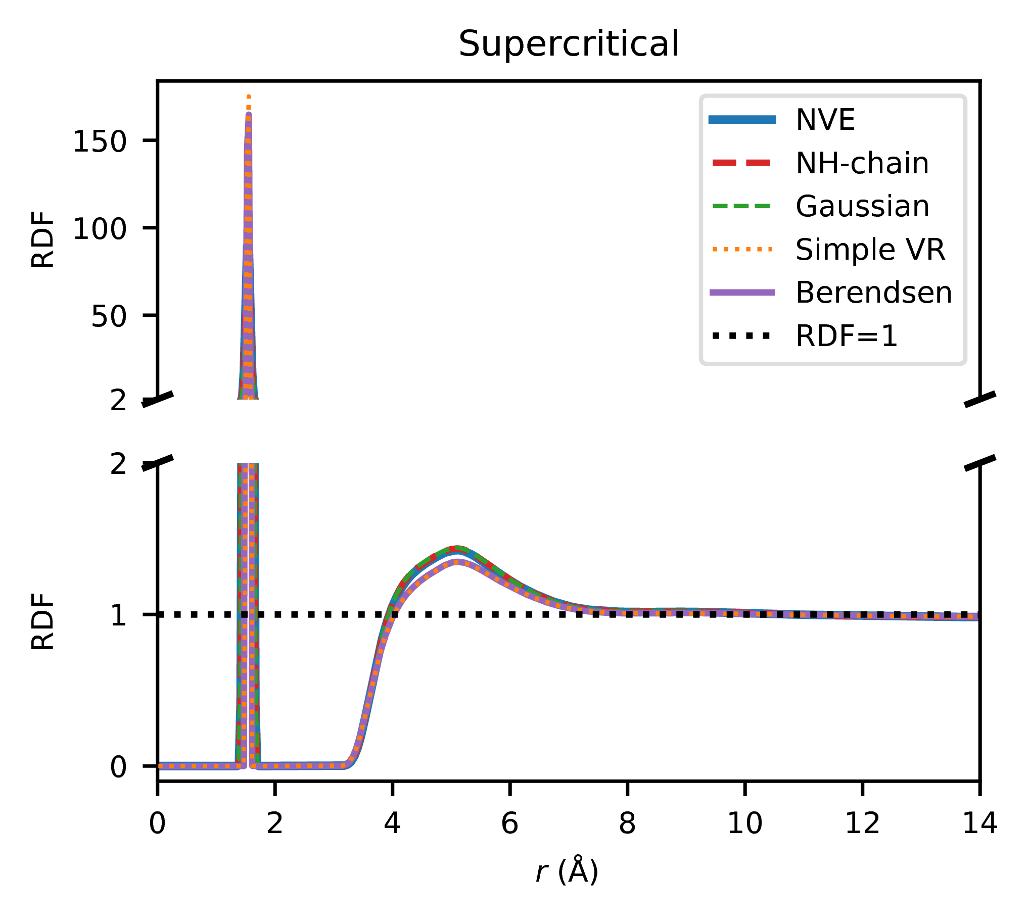
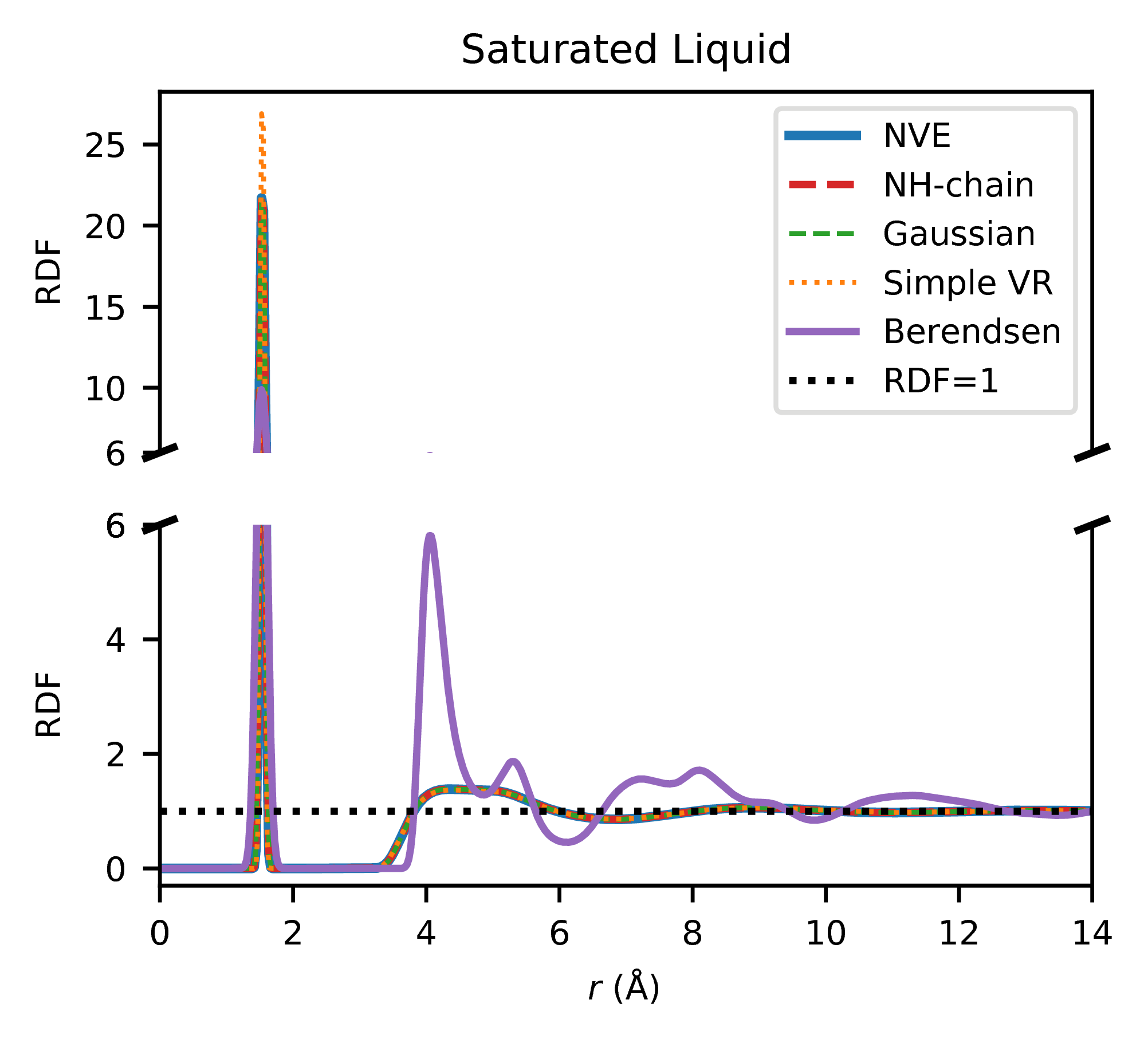
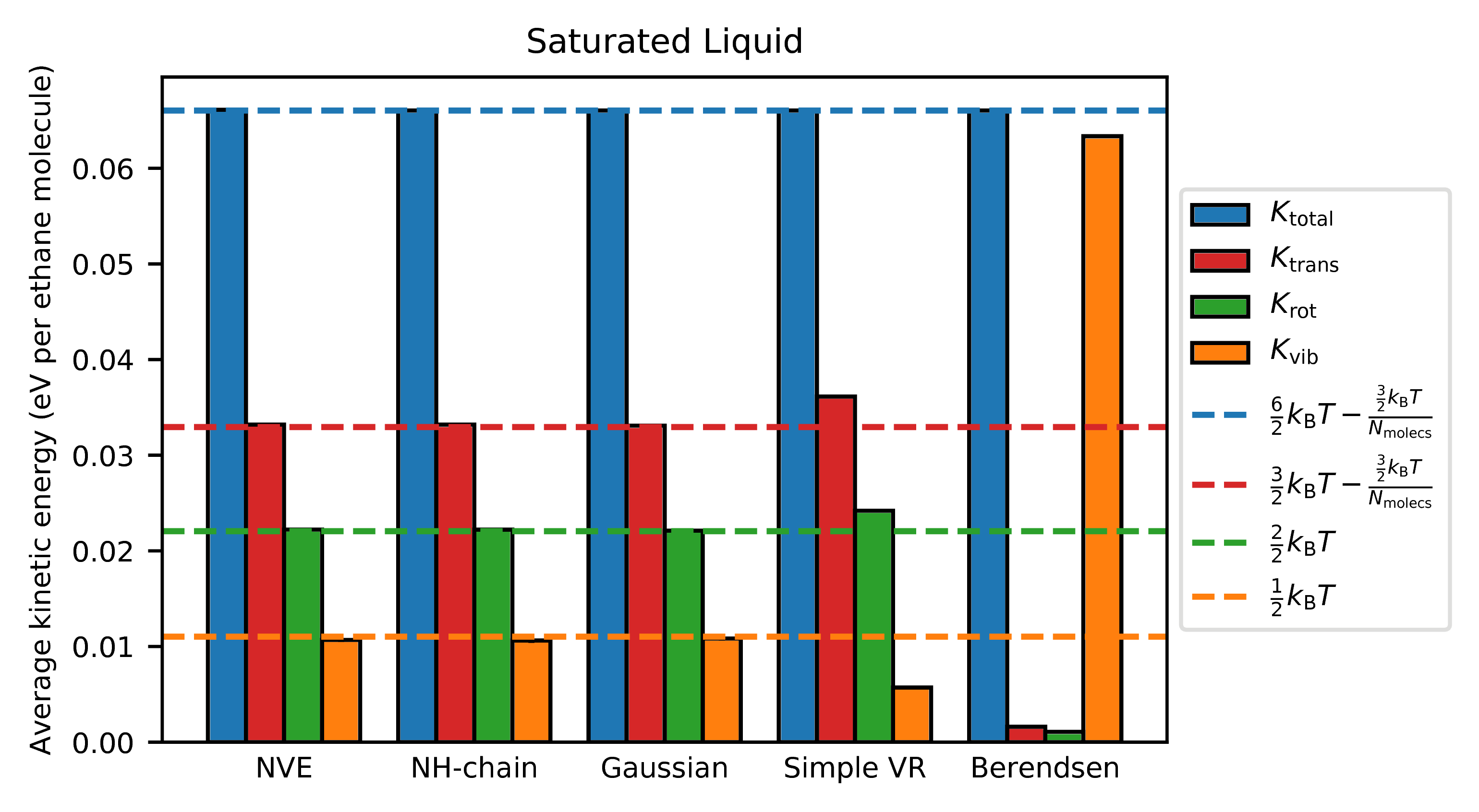
Figure 10: (top-left) Radial distribution function (RDF)of the CH3-CH3 distance obtained from the MD simulations of 50 ethane molecules in a $30\text{\,}\mathrm{\SIUnitSymbolAngstrom}$ cubic simulation box with a target temperature set to $350\text{\,}\mathrm{K}$ using various thermostats. These simulations were the same as the ones whose kinetic energy partitionings are shown in Fig. 3. (top-right) RDF of the CH3-CH3 distance obtained from MD simulations of 235 ethane molecules in a $30\text{\,}\mathrm{\SIUnitSymbolAngstrom}$ cubic simulation box with a target temperature set to $256\text{\,}\mathrm{K}$ using various thermostats. These conditions were chosen such that the simulation would take place under saturated liquid conditions.⁴⁴ For both sets of simulations, COM momentum was fixed to zero throughout. The RDFs of both sets of simulations done using the Langevin and CSVR thermostats were indistinguishable from the RDF using the Nosé-Hoover thermostat within the line width. (bottom) Partitioning of the kinetic energies obtained from the saturated liquid simulations. The results of the simulations using the Langevin and CSVR thermostats were indistinguishable from the dashed lines of equipartition within the line width.

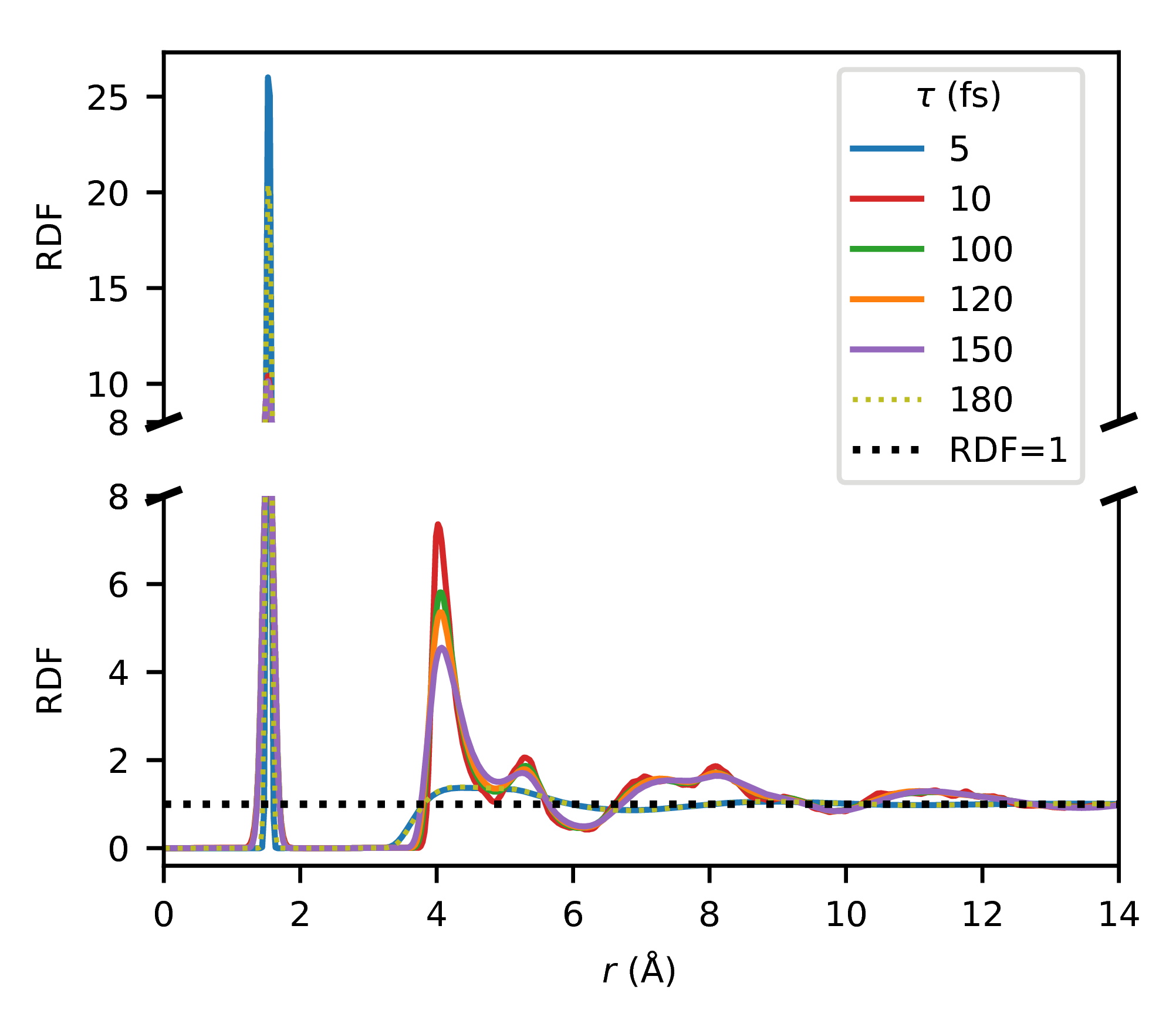
Figure 12: Similar to Fig. 10, radial distribution function (RDF)of the CH₃-CH₃ distance obtained from MD simulations of 235 ethane molecules in a $30\text{\,}\mathrm{\SIUnitSymbolAngstrom}$ cubic simulation box with a target temperature set to $256\text{\,}\mathrm{K}$ using the Berendsen thermostat with different values of the time damping constant. RDFs for simulations with the time damping constant set to $0.52\text{\,}\mathrm{fs}$ look similar to the $5\text{\,}\mathrm{fs}$ case, and RDFs for simulations with the time damping constant set to $2001000\text{\,}\mathrm{fs}$ look similar to the $180\text{\,}\mathrm{fs}$ case.

We next turn to saturated liquid phase ethane simulations, for which we show RDFs under various thermostats in Fig. 10 (top-right). The Nosé-Hoover, Langevin, CSVR, and Gaussian thermostats all give identical results typical of a simple diatomic liquid.⁵³ The simple velocity rescaling algorithm once again shows a subtle difference, but the Berendsen thermostat shows a very different RDF more reminiscent of the solid phase than the liquid phase,⁵³ and visualization of the Berendsen thermostat system shows that the ethane molecules have indeed packed into a volume smaller than available in the simulation box. Examination of the kinetic energy partitionings in Fig. 10 (bottom) shows that most of the kinetic energy is in vibrational modes, which is unexpected since that is the opposite of the usual flying ice cube result. The Berendsen thermostat’s results are heavily dependent on the choice of time damping constant, with the RDF indicating a solid-like phase for time damping constants approximately from $10150\text{\,}\mathrm{fs}$ (Fig. 12). This effect of intermediate time damping constants giving larger deviations than small or large ones has been observed before in simulations of bulk water, where the effect was attributed to the intermediate time constant matching a characteristic time scale on which dynamical correlations are most pronounced.⁵⁰ It appears clear that the Berendsen thermostat is not immune to the resonance artifacts that we have also seen with simple velocity rescaling (Fig. 7).

3.6 Contemporary use of the simple velocity rescaling and Berendsen thermostat algorithms

Ours is not the first publication to warn against the use of simple velocity rescaling and the Berendsen thermostat.^{26, 32, 54} Nonetheless, as we have stated, these algorithms continue to be widely used (Fig. 1). As we have just shown, for some systems the improper velocity rescaling algorithms may not greatly affect the system properties, and there are a slew of studies in which these thermostats are tested for specific systems, with some showing artifacts and others showing indistinguishability.^{55, 49, 50, 56, 57, 58, 35} However, slight changes to a system could introduce artifacts in an unpredictable fashion. Rather than testing for the correctness of simple velocity rescaling or the Berendsen thermostat in every specific system, we advocate for the cessation of their use. We find no reason to use simple velocity rescaling or the Berendsen thermostat instead of the CSVR thermostat given their similar ease of implementation, likely similar speeds of equilibration,⁵⁹ and our study’s finding that the CSVR thermostat does not lead to the flying ice cube effect, As a case study on the dangers of continuing to use these thermostat algorithms, we examine a highly-cited study in depth, the replication of which initially led us to examine the flying ice cube phenomenon.

In 2007, a flexible force field intended for use with MOF-5 was parameterized,⁶⁰ and it was shortly thereafter used to study the confined transport of guest molecules within the framework.⁶¹ The authors were able to replicate the experimental diffusion coefficient of confined benzene, but they found that this replicability only held when the metal-organic framework (MOF) was allowed to be flexible; when the MOF atoms were held rigid, the benzene diffusion coefficient increased by an order of magnitude. The conclusions of this manuscript are often evoked to question the validity of the rigid framework assumption that is commonly used in many MOF molecular simulation studies.

The finding continues to be accepted since it is known that the effect of framework flexibility on guest diffusion is complex,⁶² though surprise has been expressed⁶³ since a rigid lattice more typically leads to a decrease in the diffusion coefficient for tight fitting molecules.⁶² In addition, using a different flexible force field for MOF-5,⁶⁴ it was found that flexibility had little effect on the diffusion coefficient, increasing it by less than a factor of 1.5.⁶⁵

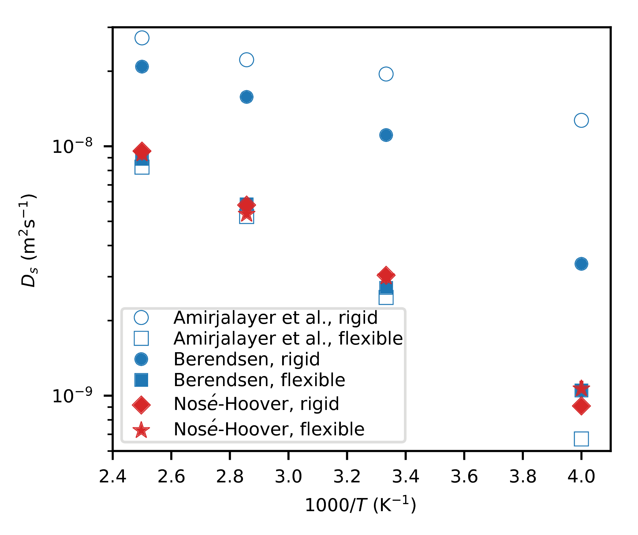
Figure 13: Identical to Fig. 11, except the Berendsen thermostat was used with a time damping constant of $200\text{\,}\mathrm{fs}$ instead of $100\text{\,}\mathrm{fs}$.

As the reader now anticipates, Amirjalayer et al. ⁶¹ used the Berendsen thermostat, which was the default option in the Tinker simulation package at the time (the default has since been changed to the CSVR thermostat).⁶⁶ As we show in Fig. 11, the result of Amirjalayer et al. ⁶¹ was completely an artifact of the Berendsen thermostat. Using the same force field, no dependence of the benzene diffusion coefficient on the framework flexibility is observed when a Nosé-Hoover or CSVR thermostat is used. Apparently, when the Berendsen thermostat is thermostatted to fewer degrees of freedom during rigid framework simulations, the flying ice cube effect becomes more noticeable and kinetic energy is drawn into the translational modes of the guest benzene molecules, accounting for the result observed by Amirjalayer et al. ⁶¹. We also found that changing the time damping constant of the Berendsen thermostat had a large effect on the diffusion coefficient (Fig. 13).

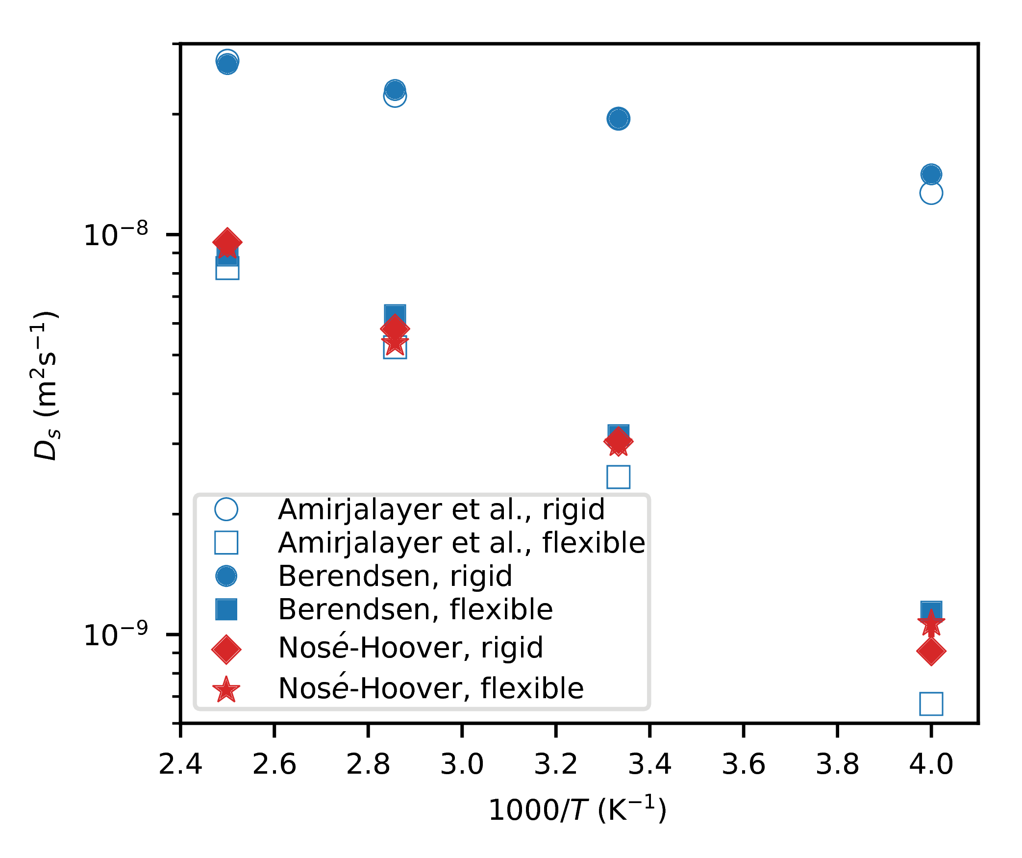
Figure 11: Self-diffusion coefficient of benzene in MOF-5 at a loading of 10 molecules per unit cell as a function of inverse temperature. Data are shown for flexible and rigid frameworks, and using the Berendsen and Nosé-Hoover chain thermostats (use of the CSVR thermostat gives diffusion coefficients that are statistically indistinguishable from use of the Nosé-Hoover thermostat). With the Berendsen thermostat, it appears that the framework flexibility has a large effect on the calculated diffusion coefficient, replicating the main finding of Amirjalayer et al. ⁶¹. However, it is seen that this result is a flying ice cube artifact, as no flexibility effect is seen with the Nosé-Hoover thermostat. Error bars represent $\pm 1$ standard error of the mean using block averaging,¹ and are not shown for the data from Amirjalayer et al. ⁶¹ or if they would be smaller than the symbol size.

As an aside, it is now known that bulk-like vapor and liquid phases of benzene exist in MOF-5 below a critical temperature.⁶⁷ It is actually improper to calculate the diffusion coefficient at a loading that is within the vapor-liquid phase envelope, e.g., $367$ molecules per unit cell at $300\text{\,}\mathrm{K}$ in this system,⁶⁷ since there is not a single homogeneous phase present at these conditions. Here, we are not attempting to calculate correct diffusion coefficients of benzene in MOF-5, but rather to compare results with the prior work of Amirjalayer et al. ⁶¹, which conducted the simulations at a loading of 10 molecules per unit cell. The importance of framework flexibility on the simulated diffusion coefficient is expected to be independent of the choice of loading.

Other errors, varying in severity, are likely present in many of the thousands of studies that have used simple velocity rescaling or the Berendsen thermostat. Occasionally, one of these errors is explicitly pointed out,^{68, 69} but negative replications are not commonly published,⁷⁰ so the extent to which these articles contain data contaminated by the flying ice cube artifact cannot be estimated.

4 Concluding Remarks

In this work, we have shown that rescaling velocities to a non-canonical distribution of kinetic energies, as is done with the simple velocity rescaling and Berendsen thermostat algorithms, causes the flying ice cube effect whereby the equipartition theorem is violated. Thus, simple velocity rescaling does not sample the isokinetic ensemble, and the Berendsen thermostat does not sample a configurational phase space intermediate between the canonical and microcanonical ensembles; justifications for their use do not hold. The flying ice cube effect is brought about by a violation of balance causing systematic redistributions of kinetic energy; this violation is lessened as the timestep between simple velocity rescalings is decreased, eventually making simple velocity rescaling equivalent to the Gaussian thermostat. Equipartition violation is completely avoided when velocities are rescaled to the canonical distribution of kinetic energies, as is done under the CSVR thermostat, because detailed balance is obeyed.

We have identified several simulation parameters which affect the prominence of the flying ice cube effect under simple velocity rescaling and the Berendsen thermostat. These include the timestep, the thermostat’s coupling strength, the frequency of collisions within the simulation (e.g., with a wall), and the system size. However, most of these parameters cannot be adjusted in a manner that eliminates the flying ice cube effect without making simulations prohibitively expensive for relevant systems of contemporary interest. Another reason not to attempt to tune these simulation parameters to allow the use of incorrect thermostatting algorithms is the existence of additional resonance artifacts that occur when the thermostat coupling strengths are set to particular values that are difficult to predict a priori.

Finally, we have demonstrated several severe simulation artifacts that the flying ice cube effect can bring about to the system’s structural and dynamic properties. These include incorrect RDFs, phase properties, and diffusion coefficients. We have highlighted one case in which the flying ice cube effect has been wholly responsible for the main finding of a highly-cited study. Many more such cases are likely present in the literature.

We strongly advocate for discontinuing use of the simple velocity rescaling and Berendsen thermostat algorithms in all MD simulations for both equilibration and production cycles. The results of past studies that have used these two algorithms should be treated with caution unless they are shown to be replicable with a more reliable thermostat. In situations where velocity rescaling methods are desirable, such as for fast equilibration of a system,⁷¹ the CSVR thermostat should be used instead.

This research was supported as part of the Center for Gas Separations Relevant to Clean Energy Technologies, an Energy Frontier Research Center funded by the U.S. Department of Energy, Office of Science, Basic Energy Sciences under Award DE-SC0001015. M.M. was supported by the Deutsche Forschungsgemeinschaft (DFG, priority program SPP 1570). This research used resources of the National Energy Research Scientific Computing Center, a DOE Office of Science User Facility supported by the Office of Science of the U.S. Department of Energy under Contract No. DE-AC02-05CH11231. E.B. thanks the responders on the LAMMPS mailing list for useful discussion and for giving advice regarding the LAMMPS source code (Axel Kohlmeyer, Steven J. Plimpton, and Aidan P. Thompson were particularly helpful) and Sai Sanigepalli for helping to implement the Tinker simulations. Special thanks go to Rochus Schmid for insightful discussion on the roles of thermostatting and for providing assistance in implementing the Tinker simulations.

Appendix A Equipartition in the isokinetic ensemble

To the best of our knowledge, it has not been shown that the equipartition theorem need necessarily apply in the isokinetic ensemble, and it is not immediately clear that it must. When additional constraints are added to the system, such as the constraint of a constant COM momentum that is typical in MD simulations with PBC or the constraint of a constant kinetic energy in the isokinetic ensemble, the change to the partition function can bring about a changed type of energy partitioning.^{29, 30}

To illustrate, we can briefly examine the former constraint of constant COM momentum, which has been analyzed before.^{28, 29, 30} One might naively think that the equipartition theorem for degrees of freedom related to the constraint (in this case, kinetic degrees of freedom, $p_{i}$) would simply change to:

$$\left<H_{p_{i}}\right>=\frac{1}{2}k_{\text{B}}T\frac{N-1}{N}$$ (8)

However, this is incorrect. Instead, it can be shown that for the canonical ensemble with its COM momentum constrained to zero, the principle of energy equipartitioning is violated for kinetic degrees of freedom.³⁰ The system instead obeys the equation:

$$\left<H_{p,i}\right>=\frac{1}{2}k_{\text{B}}T\frac{M_{\text{total}}-m_{i}}{M_{\text{total}}}$$ (9)

with a similar expression for the microcanonical ensemble when the COM momentum is constrained to zero.³⁰ For a system of equally-sized particles, the naive expression of Eq. 8 is recovered and equipartition holds, but for a system with particles of difference masses, the particles will have different amounts of kinetic energy; for a system containing massive tracer particles, the difference between the expressions can be severe.³¹ In the thermodynamic limit, the constraint of constant COM momentum does not affect the equipartition theorem.

Our equipartition theorem analysis of the isokinetic ensemble very closely follows the work of Uline et al. ³⁰ for the momentum-constrained canonical ensemble. The system to be analyzed is described by the Hamiltonian:

$$H(\mathbf{r}^{N},\mathbf{p}^{N})=\sum_{i=1}^{N}\frac{\mathbf{p}_{i}^{2}}{2m_{i}}+U(\mathbf{r}^{N})$$ (10)

The configurational part of the isokinetic ensemble’s partition function is not interesting since it is equivalent to that of the canonical ensemble’s. We will focus on the integral over momenta, or the “translational” partition function of the isokinetic ensemble:^{21, 30}

$$Q_{\text{trans}}(N,V,T,K)=\int d\mathbf{p}^{N}\exp\left(-\beta\sum_{i=1}^{N}\frac{\mathbf{p}_{i}^{2}}{2m_{i}}\right)\delta\left(K-\sum_{i=1}^{N}\frac{\mathbf{p}_{i}^{2}}{2m_{i}}\right)$$ (11)

To solve this expression, we will take the Laplace transform, integrate, and then take the inverse Laplace transform. We Laplace transform $Q_{\text{trans}}$ from $K\rightarrow s$ to obtain:

$$Q_{\text{trans}}(N,V,T,s)=\int d\mathbf{p}^{N}\exp\left(-\left(\beta+s\right)\sum_{i=1}^{N}\frac{\mathbf{p}_{i}^{2}}{2m_{i}}\right)$$ (12)

Integrating over all $\mathbf{p}_{i}$ gives:

$$Q_{\text{trans}}(N,V,T,s)=\left(2\pi\right)^{\frac{dN}{2}}\left(\prod_{i=1}^{N}m_{i}^{\frac{d}{2}}\right)\left(s+\beta\right)^{-\frac{dN}{2}}$$ (13)

The inverse Laplace transform from $s\rightarrow K$ yields:

$$Q_{\text{trans}}(N,V,T,K)=\left(2\pi\right)^{\frac{dN}{2}}\left(\prod_{i=1}^{N}m_{i}^{\frac{d}{2}}\right)\frac{\exp(-\beta K)K^{\frac{dN}{2}-1}}{\Gamma\left(\frac{dN}{2}\right)}$$ (14)

This translational partition function is then used to generate the probability distribution $f$ for a single kinetic degree of freedom, $p_{1}$:

$$f(N,V,T,K,p_{1})=\frac{\int dp^{dN-1}\exp\left(-\beta\sum_{i=1}^{dN}\frac{p_{i}^{2}}{2m_{i}}\right)\delta\left(K-\sum_{i=1}^{dN}\frac{p_{i}^{2}}{2m_{i}}\right)}{Q_{\text{trans}}(N,V,T,K)}$$ (15)

As before, we Laplace transform ($K\rightarrow s$), integrate, and inverse Laplace transform ($s\rightarrow K$) to obtain:

$$f(N,V,T,K,p_{1}) =\frac{\left(2\pi\right)^{\frac{dN-1}{2}}\frac{\left(\prod_{i=1}^{N}m_{i}^{\frac{d}{2}}\right)}{m_{1}^{\frac{1}{2}}}\frac{\exp(-\beta K)\left(K-\frac{p_{1}^{2}}{2m_{1}}\right)^{\frac{dN-1}{2}-1}\Theta\left(K-\frac{p_{1}^{2}}{2m_{1}}\right)}{\Gamma\left(\frac{dN-1}{2}\right)}}{Q_{\text{trans}}(N,V,T,K)}$$

$$=\left(2\pi m_{1}\right)^{-\frac{1}{2}}\frac{\left(K-\frac{p_{1}^{2}}{2m_{1}}\right)^{\frac{dN-1}{2}-1}}{K^{\frac{dN}{2}-1}}\frac{\Gamma\left(\frac{dN}{2}\right)}{\Gamma\left(\frac{dN-1}{2}\right)}\Theta\left(K-\frac{p_{1}^{2}}{2m_{1}}\right)$$ (16)

The presence of the Heaviside step function is a consequence of the impossibility of satisfying the kinetic energy constraint if the kinetic energy of a single degree of freedom is greater than the set total kinetic energy. The function can be integrated over $p_{1}$ by setting the integration bounds as $p_{1}=\pm\sqrt{2m_{1}K}$ to remove the Heaviside step function from the integral. It can be verified that the integral of $f(N,V,T,K,p_{1})$ over $p_{1}$ is unity.

The average kinetic energy of a kinetic degree of freedom is then:

$$\frac{<p_{1}^{2}>}{2m_{1}} =\int dp_{1}\frac{p_{1}^{2}}{2m_{1}}f(N,V,T,K,p_{1})$$

$$=\frac{K}{dN}$$ (17)

which indicates equipartition for every kinetic degree of freedom, regardless of the value of $K$. If $K$ is set to the average kinetic energy for a particular temperature, i.e., $K=\frac{d}{2}Nk_{\text{B}}T$:

$$\frac{<p_{1}^{2}>}{2m_{1}}=\frac{1}{2}k_{\text{B}}T$$ (18)

so every degree of freedom will have the same average kinetic energy as in the canonical or microcanonical ensembles.

Thus, the equipartition theorem must hold in the isokinetic ensemble.

Appendix B Partitioning kinetic energy into translational, rotational, and vibrational modes

Kinetic energies of each diatomic molecule were partitioned into translational, rotational, and vibrational kinetic energies. In one dimension, this was done as:

$$K =\frac{1}{2}m_{1}v_{1,x}^{2}+\frac{1}{2}m_{2}v_{2,x}^{2}$$

$$=\frac{1}{2}\left(m_{1}+m_{2}\right)\left(\frac{m_{1}v_{1,x}+m_{2}v_{2,x}}{m_{1}+m_{2}}\right)^{2}+\frac{1}{2}\left(\frac{m_{1}m_{2}}{m_{1}+m_{2}}\right)\left(v_{2,x}-v_{1,x}\right)^{2}$$

$$=\underbrace{\frac{1}{2}\left(m_{1}+m_{2}\right)v_{\text{trans},x}^{2}}_{K_{\rm{trans}}}+\underbrace{\frac{1}{2}\mu v_{\text{vib},x}^{2}}_{K_{\rm{vib}}}$$

where $v_{\text{trans},i}=\frac{m_{1}v_{1,i}+m_{2}v_{2,i}}{m_{1}+m_{2}}$, $v_{\text{vib},i}=v_{2,i}-v_{1,i}$, and $\mu=\frac{m_{1}m_{2}}{m_{1}+m_{2}}$, giving one translational and one vibrational degrees of freedom for the molecule. In three dimensions, this was similarly done as:

$$K =\frac{1}{2}m_{1}\left(v_{1,x}^{2}+v_{1,y}^{2}+v_{1,z}^{2}\right)+\frac{1}{2}m_{2}\left(v_{2,x}^{2}+v_{2,y}^{2}+v_{2,z}^{2}\right)$$

$$=\underbrace{\frac{1}{2}\left(m_{1}+m_{2}\right)\left(v_{\text{trans},x}^{2}+v_{\text{trans},y}^{2}+v_{\text{trans},z}^{2}\right)}_{K_{\rm{trans}}}+\underbrace{\frac{1}{2}\mu\left(\left(v_{2,x}-v_{1,x}\right)^{2}+\left(v_{2,y}-v_{1,y}\right)^{2}\right)}_{K_{\rm{rot}}}+\underbrace{\frac{1}{2}\mu\left(v_{2,z}-v_{1,z}\right)^{2}}_{K_{\rm{vib}}}$$

with an arbitrary coordinate axis aligned with the bond vector (we chose to label the equation above such that the $z$-axis was aligned), giving three translational, two rotational, and one vibrational degrees of freedom for the molecule. The code to calculate these partitioned energies was incorporated into the open-source LAMMPS code and made publicly available starting with the 2016-09-13 update as part of the “compute bond/local” command.

Appendix C Simulation details for the benzene in MOF-5 system

Simulations of benzene in MOF-5 were conducted with the Tinker package,⁶⁶ version 7.1, for the purposes of using the force field of Tafipolsky et al. ⁶⁰ to compare results with Amirjalayer et al. ⁶¹. Tinker input scripts are available in the Supplementary Information†. The force field of Tafipolsky et al. ⁶⁰ was used with the modification of using point charges instead of bond dipoles since—to the best of our knowledge—computing Ewald summations with the latter is not implemented in Tinker (it is unclear how Ewald summations were computed in Tafipolsky et al. ⁶⁰ and Amirjalayer et al. ⁶¹); we used the atomic charges that Tafipolsky et al. ⁶⁰ used to parameterize their force field, as given in their Table 2. We strived to keep conditions as similar to those used by Amirjalayer et al. ⁶¹ as possible; we used a timestep of $1\text{\,}\mathrm{fs}$, a Lennard-Jones potential cutoff of $12\text{\,}\mathrm{\SIUnitSymbolAngstrom}$, Ewald summations with default Tinker 7.1 parameters, the formerly default Berendsen thermostat time damping constant of $100\text{\,}\mathrm{fs}$ (except for where we noted that we used the currently default time damping constant of $200\text{\,}\mathrm{fs}$), and Nosé-Hoover default Tinker parameters. Simulations were run for at least $2\text{\,}\mathrm{ns}$ of equilibration and at least $100\text{\,}\mathrm{ns}$ of production, which was found to be sufficiently long for the mean-squared displacement (MSD) to become a linear function of time. Simulations were conducted in a simulation box consisting of a single cubic unit cell taken from a minimized structure described in Tafipolsky et al. ⁶⁰ and kindly supplied to us by Rochus Schmid, consisting of 424 atoms and with a lattice constant of $25.9457\text{\,}\mathrm{\SIUnitSymbolAngstrom}$. The 10 benzene molecules were distributed through the MOF-5 crystal by running a $200\text{\,}\mathrm{ps}$ MD simulation at $1000\text{\,}\mathrm{K}$ with the MOF atoms frozen prior to equilibration.

Appendix D Derivation of phase space boundaries in Fig. 5

Consider a MD simulation initially on line $\overline{CD}$ in phase space (Fig. 5). By being infinitesimally close to point $C$ when rescaling, the rescaling line will have a slope of $\frac{K_{\rm{target}}-x_{C}}{x_{C}}$. To remain moving in phase space in the direction of increasing translational kinetic energy, rescaling must continue to occur below the target isokinetic line; thus, the greatest slope that can continue to be achieved is $\frac{K_{\rm{target}}-x}{x}$. We see that the red dashed line can therefore be derived by solving the differential equation $\frac{dy_{\rm{max}}}{dx}=\frac{K_{\rm{target}}-x}{x}$ with boundary condition $y_{\rm{max}}(x_{C})=y_{C}=K_{\rm{target}}-x_{C}$, which results in $y_{\rm{max}}(x)=K_{\rm{target}}\ln{\left(\frac{x}{x_{C}}\right)}-x+K_{\rm{target}}$.

A similar situation occurs when moving in phase space in the direction of decreasing translational kinetic energy. The velocity rescaling line with smallest slope is achieved when rescaling just above the target isokinetic line, e.g., just above point $F$ when rescaling from line $\overline{AB}$. The same differential equation must be solved to derive the blue dashed line, only changing the boundary condition to $y_{\rm{max}}(x_{B})=y_{B}$, which results in $y_{\rm{max}}(x)=K_{\rm{target}}\ln{\left(\frac{x}{x_{B}}\right)}-x+x_{B}+y_{B}$. By replacing $x_{B}$ and $y_{B}$ in this equation with the beginning positions $x_{0}$ and $y_{0}=U_{\rm{max}}(x_{0})$, one obtains the general expression $y_{\rm{max}}(x)=K_{\rm{target}}\ln{\left(\frac{x}{x_{0}}\right)}-x+x_{0}+U_{\rm{max}}(x_{0})$.

Appendix E Supplementary Figures

References

- Frenkel and Smit 2002 Frenkel, D.; Smit, B. Understanding Molecular Simulation: From Algorithms to Applications; Elsevier Science, 2002
- Leimkuhler and Matthews 2015 Leimkuhler, B.; Matthews, C. In Molecular Dynamics With Deterministic and Stochastic Numerical Methods; Antman, S. S., Holmes, P., Greengard, L., Eds.; Interdisciplinary Applied Mathematics 39; Springer, 2015
- Woodcock 1971 Woodcock, L. V. Chem. Phys. Lett. 1971, 10, 257–261
- Evans \latinet al. 1983 Evans, D. J.; Hoover, W. G.; Failor, B. H.; Moran, B.; Ladd, A. J. C. Phys. Rev. A 1983, 28, 1016–1021
- Nosé 1984 Nosé, S. J. Chem. Phys. 1984, 81, 511–519
- Evans and Morriss 1990 Evans, D. J.; Morriss, G. P. Statistical Mechanics of Nonequilibrium Liquids; Theoretical Chemistry Monograph Series; Academic Press: London, 1990
- Schneider and Stoll 1978 Schneider, T.; Stoll, E. Phys. Rev. B 1978, 17, 1302–1322
- Berendsen \latinet al. 1984 Berendsen, H. J. C.; Postma, J. P. M.; van Gunsteren, W. F.; DiNola, A.; Haak, J. R. J. Chem. Phys. 1984, 81, 3684–3690
- Bussi \latinet al. 2007 Bussi, G.; Donadio, D.; Parrinello, M. J. Chem. Phys. 2007, 126, 014101
- Heyes 1983 Heyes, D. M. Chem. Phys. 1983, 82, 285–301
- Nosé 1984 Nosé, S. Mol. Phys. 1984, 52, 255–268
- Hoover 1985 Hoover, W. G. Phys. Rev. A 1985, 31, 1695–1697
- Martyna \latinet al. 1992 Martyna, G. J.; Klein, M. L.; Tuckerman, M. J. Chem. Phys. 1992, 97, 2635–2643
- Andersen 1980 Andersen, H. C. J. Chem. Phys. 1980, 72, 2384–2393
- Tobias \latinet al. 1993 Tobias, D. J.; Martyna, G. J.; Klein, M. L. J. Phys. Chem. 1993, 97, 12959–12966
- Morriss and Dettmann 1998 Morriss, G. P.; Dettmann, C. P. Chaos 1998, 8, 321–336
- Hünenberger 2005 Hünenberger, P. H. In Advanced Computer Simulation; Holm, C., Kremer, K., Eds.; Advances in Polymer Science; Springer, 2005; Vol. 173; pp 104–149
- Tuckerman 2010 Tuckerman, M. Statistical Mechanics: Theory and Molecular Simulation; Oxford Graduate Texts; Oxford University Press: Oxford, 2010
- Haile and Gupta 1983 Haile, J. M.; Gupta, S. J. Chem. Phys. 1983, 79, 3067–3076
- Evans and Morriss 1983 Evans, D. J.; Morriss, G. Phys. Lett. A 1983, 98, 433–436
- Minary \latinet al. 2003 Minary, P.; Martyna, G. J.; Tuckerman, M. E. J. Chem. Phys. 2003, 118, 2510–2526
- Collins \latinet al. 2010 Collins, P.; Ezra, G. S.; Wiggins, S. J. Chem. Phys. 2010, 133, 014105
- Morishita 2000 Morishita, T. J. Chem. Phys. 2000, 113, 2976–2982
- Morishita 2003 Morishita, T. J. Chem. Phys. 2003, 119, 7075–7082
- Lemak and Balabaev 1994 Lemak, A. S.; Balabaev, N. K. Mol. Simul. 1994, 13, 177–187
- Harvey \latinet al. 1998 Harvey, S. C.; Tan, R. K.-Z.; Cheatham, T. E. J. Comput. Chem. 1998, 19, 726–740
- Callen 1985 Callen, H. B. Thermodynamics and an Introduction to Thermostatistics, 2nd ed.; John Wiley & Sons, 1985
- Çağin and Ray 1988 Çağin, T.; Ray, J. R. Phys. Rev. A 1988, 37, 4510–4513
- Shirts \latinet al. 2006 Shirts, R. B.; Burt, S. R.; Johnson, A. M. J. Chem. Phys. 2006, 125, 164102
- Uline \latinet al. 2008 Uline, M. J.; Siderius, D. W.; Corti, D. S. J. Chem. Phys. 2008, 128, 124301
- Siboni \latinet al. 2013 Siboni, N. H.; Raabe, D.; Varnik, F. Phys. Rev. E 2013, 87, 030101
- Cooke and Schmidler 2008 Cooke, B.; Schmidler, S. C. J. Chem. Phys. 2008, 129, 164112
- Lingenheil \latinet al. 2008 Lingenheil, M.; Denschlag, R.; Reichold, R.; Tavan, P. J. Chem. Theory Comput. 2008, 4, 1293–1306
- Goga \latinet al. 2012 Goga, N.; Rzepiela, A. J.; de Vries, A. H.; Marrink, S. J.; Berendsen, H. J. C. J. Chem. Theory Comput. 2012, 8, 3637–3649
- Basconi and Shirts 2013 Basconi, J. E.; Shirts, M. R. J. Chem. Theory Comput. 2013, 9, 2887–2899
- Nosé 1991 Nosé, S. Prog. Theor. Phys. Suppl. 1991, 103, 1–46
- Chiu \latinet al. 2000 Chiu, S.; Clark, M.; Subramaniam, S.; Jakobsson, E. J. Comput. Chem. 2000, 21, 121–131
- Eastwood \latinet al. 2010 Eastwood, M. P.; Stafford, K. A.; Lippert, R. A.; Jensen, M. Ø.; Maragakis, P.; Predescu, C.; Dror, R. O.; Shaw, D. E. J. Chem. Theory Comput. 2010, 6, 2045–2058
- Sagui and Darden 1999 Sagui, C.; Darden, T. A. Annu. Rev. Biophys. Biomol. Struct. 1999, 28, 155–179
- Wagner \latinet al. 2013 Wagner, J. R.; Balaraman, G. S.; Niesen, M. J. M.; Larsen, A. B.; Jain, A.; Vaidehi, N. J. Comput. Chem. 2013, 34, 904–914
- Yan \latinet al. 2013 Yan, L.; Sun, C.; Liu, H. Adv. Manuf. 2013, 1, 160–165
- Plimpton 1995 Plimpton, S. J. Comput. Phys. 1995, 117, 1–19
- 43 We used the \DTMdate2016-11-17 release of LAMMPS to conduct our simulations. The Gaussian thermostat was not implemented in LAMMPS, so we wrote an extension that integrates the equations of motion given by Minary \latinet al. 21. This extension was later incorporated into the LAMMPS code and made publicly available starting with the \DTMdate2017-01-06 update as part of the “fix nvk” command.
- Martin and Siepmann 1998 Martin, G. M.; Siepmann, J. I. J. Phys. Chem. B 1998, 102, 2569–2577
- Toxvaerd and Olsen 1990 Toxvaerd, S.; Olsen, O. H. Phys. Scr. 1990, 1990, 98–101
- Tuckerman \latinet al. 2001 Tuckerman, M. E.; Liu, Y.; Ciccotti, G.; Martyna, G. J. J. Chem. Phys. 2001, 115, 1678–1702
- Hess 2003 Hess, S. Z. Naturforsch. A 2003, 58, 377–391
- Manousiouthakis and Deem 1999 Manousiouthakis, V. I.; Deem, M. W. J. Chem. Phys. 1999, 110, 2753–2756
- Mark and Nilsson 2002 Mark, P.; Nilsson, L. J. Comput. Chem. 2002, 23, 1211–1219
- Mudi and Chakravarty 2004 Mudi, A.; Chakravarty, C. Mol. Phys. 2004, 102, 681–685
- Berendsen \latinet al. 1981 Berendsen, H. J. C.; Postma, J. P. M.; van Gunsteren, W. F.; Hermans, J. Interaction Models for Water in Relation to Protein Hydration. Intermolecular Forces. Dordrecht, 1981; pp 331–342
- Steele 1973 Steele, W. A. Surf. Sci. 1973, 36, 317–352
- Chandler 1987 Chandler, D. Introduction to Modern Statistical Mechanics; Oxford University Press, 1987
- Shirts 2013 Shirts, M. R. J. Chem. Theory Comput. 2013, 9, 909–926
- Cheng and Merz 1996 Cheng, A.; Merz, K. M. J. Phys. Chem. 1996, 100, 1927–1937
- Mor \latinet al. 2008 Mor, A.; Ziv, G.; Levy, Y. J. Comput. Chem. 2008, 29, 1992–1998
- Rosta \latinet al. 2009 Rosta, E.; Buchete, N. V.; Hummer, G. J. Chem. Theory Comput. 2009, 5, 1393–1399
- Spill \latinet al. 2011 Spill, Y. G.; Pasquali, S.; Derreumaux, P. J. Chem. Theory Comput. 2011, 7, 1502–1510
- Bussi and Parrinello 2008 Bussi, G.; Parrinello, M. Comput. Phys. Commun. 2008, 179, 26–29
- Tafipolsky \latinet al. 2007 Tafipolsky, M.; Amirjalayer, S.; Schmid, R. J. Comput. Chem. 2007, 28, 1169–1176
- Amirjalayer \latinet al. 2007 Amirjalayer, S.; Tafipolsky, M.; Schmid, R. Angew. Chem., Int. Ed. 2007, 46, 463–466
- Smit and Maesen 2008 Smit, B.; Maesen, T. L. M. Chem. Rev. 2008, 108, 4125–4184
- Seehamart \latinet al. 2009 Seehamart, K.; Nanok, T.; Krishna, R.; van Baten, J. M.; Remsungnen, T.; Fritzsche, S. Microporous Mesoporous Mater. 2009, 125, 97–100
- Dubbeldam \latinet al. 2007 Dubbeldam, D.; Walton, K. S.; Ellis, D. E.; Snurr, R. Q. Angew. Chem. Int. Ed. 2007, 46, 4496–4499
- Ford \latinet al. 2009 Ford, D. C.; Dubbeldam, D.; Snurr, R. Q. diffusion-fundamentals.org 2009, 11, 1–8
- Ponder and Richards 1987 Ponder, J. W.; Richards, F. M. J. Comput. Chem. 1987, 8, 1016–1024
- Braun \latinet al. 2015 Braun, E.; Chen, J. J.; Schnell, S. K.; Lin, L.-C.; Reimer, J. A.; Smit, B. Angew. Chem. Int. Ed. 2015, 54, 14349–14352
- Leyssale and Vignoles 2008 Leyssale, J.-M.; Vignoles, G. L. Chem. Phys. Lett. 2008, 454, 299–304
- Wong-ekkabut \latinet al. 2010 Wong-ekkabut, J.; Miettinen, M. S.; Dias, C.; Karttunen, M. Nat. Nanotechnol. 2010, 5, 555–557
- Baker 2016 Baker, M. Nature 2016, 533, 452–454
- Hu and Sinnott 2004 Hu, Y.; Sinnott, S. B. J. Comput. Phys. 2004, 200, 251–266