Clustering With Pairwise Relationships:
A Generative Approach

Abstract

Semi-supervised learning (SSL) has become important in current data analysis applications, where the amount of unlabeled data is growing exponentially and user input remains limited by logistics and expense. Constrained clustering, as a subclass of SSL, makes use of user input in the form of relationships between data points (e.g., pairs of data points belonging to the same class or different classes) and can remarkably improve the performance of unsupervised clustering in order to reflect user-defined knowledge of the relationships between particular data points. Existing algorithms incorporate such user input, heuristically, as either hard constraints or soft penalties, which are separate from any generative or statistical aspect of the clustering model; this results in formulations that are suboptimal and not sufficiently general. In this paper, we propose a principled, generative approach to probabilistically model, without ad hoc penalties, the joint distribution given by user-defined pairwise relations. The proposed model accounts for general underlying distributions without assuming a specific form and relies on expectation-maximization for model fitting. For distributions in a standard form, the proposed approach results in a closed-form solution for updated parameters. Results demonstrate the proposed model reflects user preferences with fewer user-defined relations compared to the state-of-the-art.

1 Introduction

Semi-supervised learning (SSL) has become a topic of significant recent interest in the context of applied machine learning, where per-class distributions are difficult to automatically separate due to limited sampling and/or limitations of the underlying mathematical model. Several applications, including content-based retrieval [51], email classification [24], gene function prediction [34], and natural language processing [40, 26], benefit from the availability of user-defined/application-specific knowledge in the presence of large amounts of complex unlabeled data, where labeled observations are often limited and expensive to acquire. In general, SSL algorithms fall into two broad categories: classification and clustering. Semi-supervised classification is considered to improve supervised classification when small amounts of labeled data with large amounts of unlabeled data are available  [53, 7]. For example, in a semi-supervised email classification, one may wish to classify constantly increasing email messages into spam/nonspam with the knowledge of a limited amount of user-/human-based classified messages [24]. On the other hand, semi-supervised clustering (SSC), also known as constrained clustering [6], aims to provide better performance for unsupervised clustering when user-based information about the relationships within a small subset of the observations becomes available. Such relations would involve data points belonging to the same or different classes. For example, a language-specific grammar is necessary in cognitive science when individuals are attempting to learn a foreign language efficiently. Such a grammar provides rules for prepositions that can be considered as user-defined knowledge for improving the ability to learn a new language.

To highlight the role of user-defined relationships for learning an application-specific data distribution, we consider the example in Figure 1(a), which shows a maximum likelihood model estimate of a Gaussian mixture that is well supported by the data. However, an application may benefit from another good (but not optimal w.r.t. likelihood) solution as in Figure 1(b), which is inconsistent with the data, but is optimal without some information in addition to the raw data points. Using a limited amount of labeled data and a large amount of unlabeled data could be difficult to guide the learning algorithm in the application-specific direction [53, 10, 29, 50], because performance of a generative model depends on the ratio of the labeled data to unlabeled data. In contrast, previous works have shown that SSC achieves the estimate in Figure 1(b), given the observed data and a small number of user-defined relationships that would guide the parameter estimation process toward a model [6] that is not only informed by the data, but also by this small amount of user input. This paper addresses the problem of incorporating such user-specific relations into a clustering problem in an effective, general, and reliable manner.

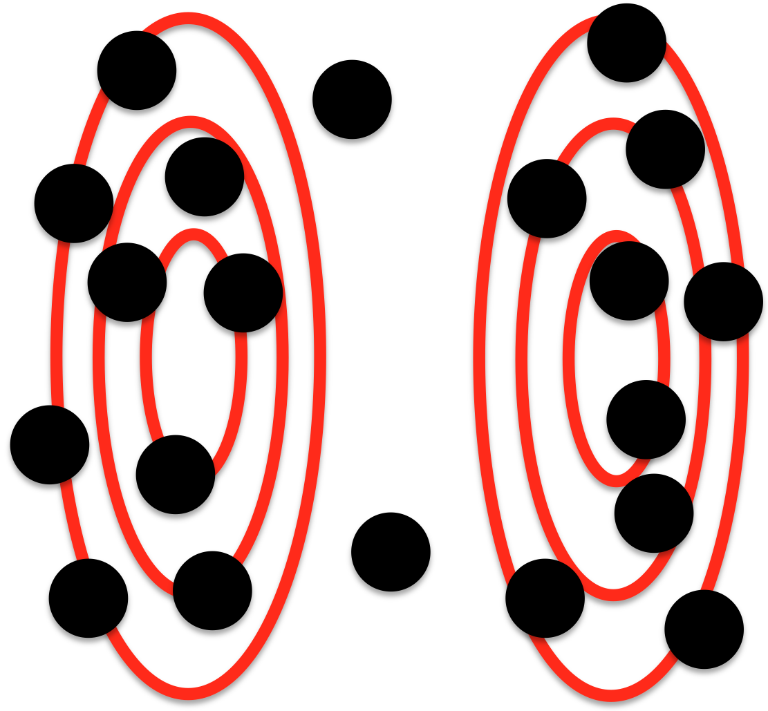
(a) Mathematically Ideal Model (b) Application-Specific Model

Figure 1: Generative model clustering example: Because of finite sampling and modeling limitations, a distribution of points may give rise to optimal solutions that, depending on the model and the data, (a) are not well suited to the application and/or (b) are not consistent with the underlying generative model, which may require domain knowledge from a user.

Clustering data using a generative framework has some useful, important properties, including compact representations, parameter estimation for subsequent statistical analysis, and the ability to induce classifications of unseen data [54]. For the problem of estimating the parameters of generative models, the expectation-maximization (EM) algorithm [13] is particularly effective. The EM formulation is guaranteed to give maximum-likelihood (ML) estimates in the unimodal case and local maxima in likelihood otherwise. Therefore, EM formulations of parameter estimation that properly account for user input in the context of SSC are of interest and one of the contributions of this paper.

A flexible and efficient way to incorporate user input into SSC is in the form of relations between observed data points, in order to define statistical relationships among observations (rather than explicit labeling, as would be done in classification). A typical example would be for a user to examine a small subset of data and decide that some pairs of points should be in different classes, referred to as a cannot-link relation, and that other pairs of data points should be in the same class, i.e., must-link. Using these basic primitives, one may build up more complex relationships among sets of points. The concept of pairwise links was first applied to centroid-based clustering approaches, for instance, in the form of constrained K-means [43], where each observation is assigned to the nearest cluster in a manner that avoids violating constraints.

Although some progress has been made in developing mechanisms for incorporating this type of user input into clustering algorithms, the need remains for a systematic, general framework that generalizes with a limited amount of user knowledge. Most state-of-the-art techniques propose adding hard constraints [38], where data points that violate the constraints do not contribute (i.e., all pairwise constraints must be satisfied), or soft penalties [30], which penalize the clustering results based on the number of violated constraints. Both hard constraints and soft penalties can lead to both a lack of generality and suboptimal solutions. For instance, in constrained K-means, introducing constraints by merely assigning a relatively small number of points to appropriate centroids does not ensure that the models (centroids) adequately respond to this user input.

In this paper, we propose a novel, generative approach for clustering with pairwise relations that incorporates these relations into the estimation process in a precise manner. The parameters are estimated by optimizing the data likelihood under the assumption that individual data points are either independent samples (as in the unsupervised case) or that they have a nontrivial joint distribution, which is determined by user input. The proposed model explicitly incorporates the pairwise relationship as a property of the generative model that guides the parameter estimation process to reflect user preferences and estimates the global structure of the underlying distribution. Moreover, the proposed model is represented as a probability distribution that can be virtually any form. The results in this paper demonstrate that the proposed optimal strategy pays off, and that it outperforms the state-of-the art on real-world datasets with significantly less user input.

2 Related Work

Semi-supervised clustering methods typically fall into one of two categories [6]: distance-based methods and constraint-based methods. The distance-based approaches combine conventional clustering algorithms with distance metrics that are designed to satisfy the information given by user input [47, 4, 45, 8]. The metrics effectively embed the points into spaces where the distances between the points with constraints are either larger or smaller to reflect the user-specified relationships. On the other hand, constraint-based algorithms incorporate the pairwise constraints into the clustering objective function, to either enforce the constraints or penalize their violation. For example,Wagstaff et al. proposed the constrained K-means algorithm, which enforced user input as hard constraints in a nonprobabilistic manner as the part of the algorithm that assigns points to classes [43]. Basu el al. proposed a probabilistic framework based on a hidden Markov random field, with ad hoc soft penalties, which integrated metric learning with the constrained K-means approach, optimized by an EM-like algorithm [5]. This work also can be applied to a kernel feature space as in [23]. Allab and Benabdeslem adapted topological clustering to pairwise constraints using a self-organizing map in a deterministic manner [2].

Semi-supervised clustering methods with generative, parametric clustering approaches have also been augmented to accommodate user input. Lu and Leen proposed a penalized clustering algorithm using Gaussian mixture models (GMM) by incorporating the pairwise constraints as a prior distribution over the latent variable directly, resulting in a computationally challenging evaluation of the posterior [30]. Such a penalization-based formulation results in a model with no clear generative interpretation and a stochastic expectation step that requires Gibbs sampling. Shental et al. proposed a GMM with equivalence constraints that defines the data from either the same or a different source. However, for the cannot-link case, they used the Markov network to describe the dependence between a pair of latent variables and sought the optimal parameter by gradient ascent [38]. Their results showed that the cannot-link relationship was unable to impact the final parameter estimation (i.e., such a relation was ineffective). Further, they imposed user input as hard constraints where data points that violate the constraints did not contribute to the parameter estimation process. A similar approach, in [25], proposed to treat the constraint as an additional random variable that increases the complexity of the optimization process. Further, their approach focused only on must-link. In this paper, we propose a novel solution to incorporating user-defined data relationships into clustering problems, so that cannot-link and must-link relations can be included in a unified framework in a way that they are computed efficiently using an EM algorithm with very modest computational demands. Moreover, the proposed formulation is general in that it can 1) accommodate any kind of relation that can be expressed as a joint probability and 2) incorporate, in principle, any probability distribution (generative model). For GMMs, however, this formulation results in a particularly attractive algorithm that entails a closed-form solution for the mean and covariance and a relatively inexpensive, iterative, constrained, nonlinear optimization for the mixing parameters.

Recently, EM-like algorithms for SSL (and clustering in particular) have received significant attention in natural language processing [20, 31]. Graca et al. proposed an EM approach with a posterior constraint that incorporates the expected values of specially designed auxiliary functions of the latent variables to influence the posterior distribution to favor user input [20]. Because of the lack of probabilistic interpretation, the expectation step is not influenced by user input, and the results are not optimal.

Unlike the generative approach, graph-based methods group the data points according to similarity and do not necessarily assume an underlying distribution. Graph-based, semi-supervised clustering methods have been demonstrated to be promising when user input is available  [52, 44, 49]. However, graph-based methods are not ideal classifiers when a new data point is presented due to their transductive property, i.e., unable to learn the general rule from the specific training data  [16, 54]. In order to classify a new data point, other than rebuilding the graph with the new data point, one likely solution is to build a separate inductive model on top of the output of the graph-based method (e.g., K-means or GMM); user input would need to be incorporated into this new model.

The work in this paper is distinct from the aforementioned works in the following aspects:

• We present a fully generative approach, rather than a heuristic approach of imposing hard constraints or adding ad hoc penalties.

• The proposed generative model reflects user preferences while maintaining a probabilistic interpretation, which allows it to be generalized to take advantage of alternative density models or optimization algorithms.

• The proposed model clearly deals with the must-link and cannot-link cases in a unified framework and demonstrates that solutions using must-link and cannot-link together or independently are tractable and effective.

• Instead of pairwise constraints, the statistical interpretation of pairwise relationships allows the model estimation to converge to a distribution that follows user preferences with less domain knowledge.

• In the proposed algorithm, the parameter estimation is very similar to a standard EM in terms of ease of implementation and efficiency.

3 Clustering With Pairwise Relationships

The proposed model incorporates user input in the form of relations between pairs of points that are in the same class (must-link) or different classes (cannot-link). The must-link and cannot-link relationships are a natural and practical choice since the user can guide the clustering without having a specific preconceived notion of classes. These pairwise relationships are typically not sufficiently dense or complete to build a full discriminative model, and yet they may be helpful in discovering the underlying structure of the unlabeled data. For data points that have no user input, we assume that they are independent, random samples. The pairwise relationships give rise to an associate generative model with a joint distribution that reflects the nature of the user input.

The parameters are estimated as an ML formulation through an EM algorithm that discovers the global structure of the underlying distribution that reflects the user-defined relations. Unlike previous works that include user input in a specific model (e.g., a GMM) through either hard constraints  [38] or soft penalties  [30], in this work we propose an ML estimation based on a generative model, without ad hoc penalties.

3.1 Generative Models: Unsupervised Scenario

In this section, we first introduce generative models for an unsupervised scenario. Suppose the unconstrained generative model consists of $M$ classes. $\mathcal{X}=\{\mathbf{x}_{n}\in\mathbb{R}^{d}\}_{n=1}^{N}$ denotes the observed dataset without user input. Dataset $\mathcal{X}$ is associated with latent set $\mathcal{Z}=\{\mathbf{z}_{n}\}_{n=1}^{N}$ where $\mathbf{z}_{n}=[z_{n}^{1},...,z_{n}^{M}]^{T}\in\{0,1\}^{M}$ with $z_{n}^{m}=1$ if and only if the corresponding data point $\mathbf{x}_{n}$ was generated from the $m$th class, subject to $\sum_{m=1}^{M}z_{n}^{m}=1$. Therefore, we can obtain the soft label for a data point $\mathbf{x}$ by estimating $p(z^{m}|\mathbf{x})$. The probability that a data point $\mathbf{x}$ is generated from a generative model with parameters $\boldsymbol{\vartheta}$ is

$$p(\mathbf{x}|\boldsymbol{\vartheta}) =\sum_{\mathbf{z}}p(\mathbf{x}|\mathbf{z},\boldsymbol{\vartheta})p(\mathbf{z})$$ (1)

The likelihood of the observed data points governed by the model parameters is

$$\mathcal{L}(\mathcal{X},\mathcal{Z},\boldsymbol{\vartheta}):=p(\mathcal{X},\mathcal{Z}|\boldsymbol{\vartheta})=\prod_{m=1}^{M}\prod_{n\in[1,N]:z_{n}^{m}=1}p(\mathbf{x}_{n})$$ (2)

$$=\prod_{m=1}^{M}\prod_{n=1}^{N}p(\mathbf{x}_{n},z_{n}^{m})=\prod_{m=1}^{M}\prod_{n=1}^{N}\bigg{[}p(\mathbf{x}_{n}|z_{n}^{m},\boldsymbol{\vartheta})p(z_{n}^{m})\bigg{]}^{z_{n}^{m}}$$ (3)

where the condition on the product term in equation (2) is restricted to data points $\mathbf{x}_{n}$ generated from the $m$th class. The joint probability in equation (3) is expressed, using Bayes’ rule, in terms of the conditional probability $p(\mathbf{x}_{n}|z_{n}^{m},\boldsymbol{\vartheta})$ and the $m$th class prior probability $p(z_{n}^{m})$. In the rest of the formulation, to simplify the representation, we use $p(\mathbf{x}_{n}|z_{n}^{m})=p(\mathbf{x}_{n}|z_{n}^{m},\boldsymbol{\vartheta})$

3.2 Generative Model With Pairwise Relationships

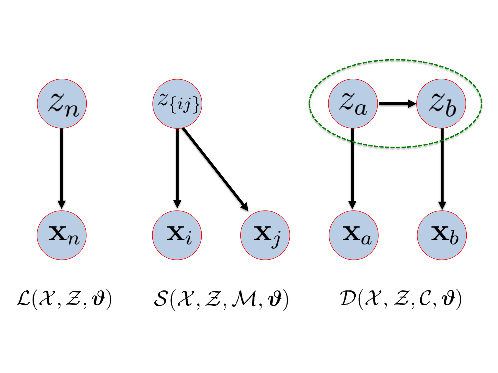
Figure 2: The graphical representation of the proposed generative model with complete data-likelihood $p(\mathcal{X},\mathcal{Z}|\mathcal{M},\mathcal{C},\boldsymbol{\vartheta})$. The $\mathcal{L}(\cdot)$ is from the standard generative model with independent samples. The $\mathcal{S}(\cdot)$ shows the must-link data points pair $\mathbf{x}_{i}$ and $\mathbf{x}_{j}$ shares a single latent variable $z_{\{ij\}}$. The $\mathcal{D}(\cdot)$ shows the cannot-link data points pair $\mathbf{x}_{a}$ and $\mathbf{x}_{b}$, where the green dashed line indicates the joint probability of $z_{a}$ and $z_{b}$.

The definition of a pairwise relation in the proposed generative model is similar to that in the unsupervised case, yet such relations are propagated to the latent variables level. In particular, $\mathcal{M}=\{(i,j)\}$ denotes a set of must-link relations where the pair $\mathbf{x}_{i}$ and $\mathbf{x}_{j}$ was generated from the same class; hence, the pair $(\mathbf{x}_{i},\mathbf{x}_{j})$ shares a single latent variable $\mathbf{z}_{\{ij\}}$. The same logic is applied to the cannot-link relations where $\mathcal{C}=\{(a,b)\}$ denotes a set of cannot-link relations encoding that $\mathbf{x}_{a}$ and $\mathbf{x}_{b}$ were generated from distinct classes; therefore, $\mathbf{z}_{a}\neq\mathbf{z}_{b}$. Including $\mathcal{M}$ and $\mathcal{C}$, the data points are now expanded to be $\mathcal{X}:=\{\mathbf{x}_{1},\dots\mathbf{x}_{N},\mathcal{M},\mathcal{C}\}$. Thus, the modified complete-data likelihood function $\mathcal{J}(\cdot)$ that would reflect user input is (refer to Figure 2 for the graphical representation)

$$\mathcal{J}(\mathcal{X},\mathcal{Z},\mathcal{M},\mathcal{C},\boldsymbol{\vartheta}) :=p(\mathcal{X},\mathcal{Z}|\mathcal{M},\mathcal{C},\boldsymbol{\vartheta})$$

$$=\mathcal{L}(\mathcal{X},\mathcal{Z},\boldsymbol{\vartheta})~{}\mathcal{S}(\mathcal{X},\mathcal{Z},\mathcal{M},\boldsymbol{\vartheta})~{}\mathcal{D}(\mathcal{X},\mathcal{Z},\mathcal{C},\boldsymbol{\vartheta}).$$ (4)

$\mathcal{S}(\cdot)$ and $\mathcal{D}(\cdot)$ are the likelihood of pairwise data points. The likelihood of the set of all pairs of must-link data points $\mathcal{S}$ is, therefore,

$$\mathcal{S}(\mathcal{X},\mathcal{Z},\mathcal{M},\boldsymbol{\vartheta}) :=p(\mathcal{X},\mathcal{Z}|\mathcal{M},\boldsymbol{\vartheta})$$

$$=\prod_{m=1}^{M}\prod_{(i,j)\in\mathcal{M}}p(\mathbf{x}_{i},\mathbf{x}_{j},z_{\{ij\}}^{m})$$

$$=\prod_{m=1}^{M}\prod_{(i,j)\in\mathcal{M}}\bigg{[}p(\mathbf{x}_{i}|z_{\{ij\}}^{m})p(\mathbf{x}_{j}|z_{\{ij\}}^{m})p(z_{\{ij\}}^{m})\bigg{]}^{z_{\{ij\}}^{m}}$$ (5)

The likelihood of the cannot-link data points explicitly reflects the fact that they are drawn from distinct classes. Therefore, the joint probability of the labeling vectors $\mathbf{z}_{a}$ and $\mathbf{z}_{b}$ for all $(a,b)\in\mathcal{C}$ is as follows:

$$p(z_{a}^{m},z_{b}^{m}) := p(z_{a}^{m}|z_{b}^{m})p(z_{b}^{m})=p(z_{b}^{m}|z_{a}^{m})p(z_{a}^{m})~{}~{}$$ (6)

$$= \left\{\begin{array}[]{ll}\cfrac{p(z_{a}^{m})^{z_{a}^{m}}p(z_{b}^{m})^{z_{b}^{m}}}{1-\sum_{m^{\prime}=1}^{M}p(z_{a}^{m^{\prime}})^{2}}&z_{a}^{m}\neq z_{b}^{m}\\ 0&z_{a}^{m}=z_{b}^{m}\\ \end{array}\right.$$ (9)

$$= \cfrac{(1-z_{a}^{m}z_{b}^{m})p(z_{a}^{m})^{z_{a}^{m}}p(z_{b}^{m})^{z_{b}^{m}}}{1-\sum_{m^{\prime}=1}^{M}p(z_{a}^{m^{\prime}})^{2}}$$ (10)

The proposed joint distribution reflects the cannot-link constraints by assigning a zero joint probability of $\mathbf{x}_{a}$ and $\mathbf{x}_{b}$ being generated from the same class, and takes into account the effect of this relation on the normalization term of the joint distribution $p(z_{a}^{m},z_{b}^{m})$. As such, the cannot-link relations contribute to the posterior distribution as follows:

$$\mathcal{D}(\mathcal{X},\mathcal{Z},\mathcal{C},\boldsymbol{\vartheta}) :=p(\mathcal{X},\mathcal{Z}|\mathcal{C},\boldsymbol{\vartheta})$$

$$=\prod_{m=1}^{M}\prod_{(a,b)\in\mathcal{C}}p(\mathbf{x}_{a},\mathbf{x}_{b},z_{a}^{m},z_{b}^{m})$$

$$=\prod_{m=1}^{M}\prod_{(a,b)\in\mathcal{C}}\Big{[}p(\mathbf{x}_{a}|z_{a}^{m})\Big{]}^{z_{a}^{m}}\Big{[}p(\mathbf{x}_{b}|z_{b}^{m})\Big{]}^{z_{b}^{m}}p(z_{a}^{m},z_{b}^{m})$$ (11)

3.3 Expectation Maximization With Pairwise Relationships

Given the joint distribution $p(\mathcal{X},\mathcal{Z}|\mathcal{M},\mathcal{C},\boldsymbol{\vartheta})$, the objective is to maximize the log-likelihood function $\log\mathcal{J}$ with respect to the parameters $\boldsymbol{\vartheta}$ of the generative process in a manner that would discover the global structure of the underlying distribution and reflect user input. This objective can be achieved using an EM algorithm.

3.3.1 E-Step

In the E-step, we estimate the posterior of the latent variables using the current parameter values $\boldsymbol{\vartheta}^{\text{old}}$.

$$\mathcal{Q}(\boldsymbol{\vartheta},\boldsymbol{\vartheta}^{\text{old}}) =\mathbb{E}_{\mathcal{Z}}[\log~{}\mathcal{J}]$$

$$=\sum_{\mathcal{Z}}p(\mathcal{Z}|\mathcal{X},\mathcal{M},\mathcal{C},\boldsymbol{\vartheta}^{\text{old}})\log p(\mathcal{X},\mathcal{Z}|\mathcal{M},\mathcal{C},\boldsymbol{\vartheta})$$ (12)

$\mathcal{L}(\cdot)$-term: Taking the expectation of $\log\mathcal{L}$ with respect to the posterior distribution of $z_{n}^{m}$ and bearing in mind that the latent variable $\mathbf{z}$ is a binary variable,

$$\mathbb{E}_{z_{n}^{m}|\mathbf{x}_{n}}[z_{n}^{m}]=\frac{p(\mathbf{x}_{n}|z_{n}^{m})p(z_{n}^{m})}{\sum_{m^{\prime}=1}^{M}p(\mathbf{x}_{n}|z_{n}^{m^{\prime}})p(z_{n}^{m^{\prime}})}$$ (13)

$\mathcal{S}(\cdot)$-term: Taking the expectation of $\log\mathcal{S}$ with respect to the must-link posterior distribution of $z^{m}_{\{ij\}}$ results in

$$\mathbb{E}_{z^{m}_{\{ij\}}|\mathbf{x}_{i},\mathbf{x}_{j}} [z^{m}_{\{ij\}}]=\frac{p(\mathbf{x}_{i}|z^{m}_{\{ij\}})p(\mathbf{x}_{j}|z^{m}_{\{ij\}})p(z^{m}_{\{ij\}})}{\sum_{m^{\prime}=1}^{M}p(\mathbf{x}_{i}|z^{m^{\prime}}_{\{ij\}})p(\mathbf{x}_{j}|z^{m^{\prime}}_{\{ij\}})p(z^{m^{\prime}}_{\{ij\}})}$$ (14)

$\mathcal{D}(\cdot)$-term: Because the proposed model does not allow $\mathbf{x}_{a}$ and $\mathbf{x}_{b}$ to be from the same class, the expectation of equation (10) in the $\log\mathcal{D}$ that both will have the same class assignment vanishes, which can be shown using Jensen’s inequality as follows:

$$\mathbb{E}_{z^{m}_{a},z^{m}_{b}|\mathbf{x}_{a},\mathbf{x}_{b}}[\log(1-z_{a}^{m}z_{b}^{m})] \leq\log\big{(}1-\mathbb{E}_{z^{m}_{a},z^{m}_{b}|\mathbf{x}_{a},\mathbf{x}_{b}}[z_{a}^{m}z_{b}^{m}]\big{)}=\log(1-0)=0$$ (15)

Hence, we can set $\log(1-z_{a}^{m}z_{b}^{m})=0$ in equation (10). The expectation of the $\log\mathcal{D}$ term with respect to $z^{m}_{a}$ is

$$\mathbb{E}_{z^{m}_{a}|\mathbf{x}_{a},\mathbf{x}_{b}}[z_{a}^{m}] =p(z_{a}^{m}|\mathbf{x}_{a},\mathbf{x}_{b})=\sum_{m^{\prime}=1}^{M}p(z_{a}^{m},z_{b}^{m^{\prime}}|\mathbf{x}_{a},\mathbf{x}_{b})$$

$$=\frac{\sum_{m^{\prime}=1}^{M}p(\mathbf{x}_{a}|z_{a}^{m})p(\mathbf{x}_{b}|z_{b}^{m^{\prime}})p(z_{a}^{m},z_{b}^{m^{\prime}})}{\sum_{m^{\prime\prime}=1}^{M}\sum_{m^{\prime\prime\prime}=1}^{M}p(\mathbf{x}_{a}|z_{a}^{m_{k}^{\prime\prime}})p(\mathbf{x}_{b}|z_{b}^{m_{k}^{\prime\prime\prime}})p(z_{a}^{m^{\prime\prime}},z_{b}^{m^{\prime\prime\prime}})}.$$ (16)

In a like manner, we can write down the expectation of $z_{b}^{m}$.

3.3.2 M-Step

In the M-step, therefore, we update the $\boldsymbol{\vartheta}^{\text{new}}$ by maximizing equation (3.3.1) and fixing the posterior distribution that we estimated in the E-step.

$$\boldsymbol{\vartheta}^{\text{new}}=\arg\max_{\boldsymbol{\vartheta}}~{}~{}\mathcal{Q}(\boldsymbol{\vartheta},\boldsymbol{\vartheta}^{\text{old}})$$ (17)

Different density models result in different update mechanisms for the respective model parameters. In the next subsection, we elaborate on an example of the proposed model to illustrate the idea of the M-step for the case of Gaussian mixture models.

3.4 Gaussian Mixture Model With Pairwise Relationships

Consider employing a single distribution (e.g., a Gaussian distribuion) for each class probability $p(\mathbf{x}|z^{m})$. The proposed model, therefore, becomes the Gaussian mixture model (GMM) with pairwise relationships. The parameter of the GMM is $\boldsymbol{\vartheta}=\{\alpha_{m},\boldsymbol{\mu}_{m},\boldsymbol{\Sigma}_{m}\}_{m=1}^{M}$, such that $\alpha_{m}\in[0,1]$ is the mixing parameter for the class proportion subject to $\sum_{m=1}^{M}\alpha_{m}=1$ and $p(z^{m})=\alpha_{m}$. $\boldsymbol{\mu}_{m}\in\mathbb{R}^{d}$ is the mean parameter, and $\boldsymbol{\Sigma}_{m}\in\mathbb{R}^{d\times d}$ is the covariance associated with the $m$th class. By taking the derivative of equation (3.3.1) with respect to $\boldsymbol{\mu}_{m}$ and $\boldsymbol{\Sigma}_{m}$, we can get

$$\boldsymbol{\mu}_{m} =\bigg{(}\sum_{n=1}^{N}\ell_{n}^{m}\mathbf{x}_{n}+\sum_{(i,j)\in\mathcal{M}}s_{ij}^{m}\big{[}\mathbf{x}_{i}+\mathbf{x}_{j}\big{]}+\sum_{(a,b)\in\mathcal{C}}\big{[}d_{a}^{m}\mathbf{x}_{a}+d_{b}^{m}\mathbf{x}_{b}\big{]}\bigg{)}\bigg{/}Z$$ (18)

$$\boldsymbol{\Sigma}_{m} =\bigg{(}\sum_{n=1}^{N}\ell_{n}^{m}\mathbf{S}_{n}^{m}+\sum_{(i,j)\in\mathcal{M}}s_{ij}^{m}\big{[}\mathbf{S}_{i}^{m}+\mathbf{S}_{j}^{m}\big{]}+\sum_{(a,b)\in\mathcal{C}}\big{[}d_{a}^{m}\mathbf{S}_{a}^{m}+d_{b}^{m}\mathbf{S}_{b}^{m}\big{]}\bigg{)}\bigg{/}Z$$ (19)

$$Z =\sum_{n=1}^{N}\ell_{n}^{m}+2\sum_{(i,j)\in\mathcal{M}}s_{ij}^{m}+\sum_{(a,b)\in\mathcal{C}}\big{[}d_{a}^{m}+d_{b}^{m}\big{]}$$ (20)

where $\ell_{n}^{m}=p(z_{n}^{m}|\mathbf{x}_{n})$, $s_{ij}^{m}=p(z_{\{ij\}}^{m}|\mathbf{x}_{i},\mathbf{x}_{j})$, $d_{a}^{m}=p(z_{a}^{m}|\mathbf{x}_{a},\mathbf{x}_{b})$ and the sample covariance $\mathbf{S}_{n}^{m}=(\mathbf{x}_{n}-\boldsymbol{\mu}_{m})(\mathbf{x}_{n}-\boldsymbol{\mu}_{m})^{T}$.

Estimating the mixing parameters $\alpha_{m}$, on the other hand, entails the following constrained nonlinear optimization, which can be solved using sequential quadratic programming with Newton-Raphson steps [15, 1]. Let $\boldsymbol{\alpha}\in\mathbb{R}^{M}$ denote the vector of mixing parameters. Given the current estimate of the mean vectors and covariance matrices, the new estimate of the mixing parameters can be solved for using the optimization problem defined in (3.4),

$$\boldsymbol{\alpha}^{*} =\arg\min_{\boldsymbol{\alpha}}-\mathcal{Q}(\boldsymbol{\vartheta},\boldsymbol{\vartheta}^{\text{old}})$$

$$\operatorname{s.t.} ~{}~{}~{}~{}~{}\mathbf{1}^{T}\boldsymbol{\alpha}-1=0~{}~{}\operatorname{and}~{}~{}\alpha_{m}\geq 0~{}~{}\forall m\in[1,M]$$ (21)

where the initialization can be obtained using the closed-form solution obtained from discarding the nonlinear part, which ignores the normalization term $\log(1-\sum_{m^{\prime}=1}^{M}\alpha_{m^{\prime}}^{2})$. The energy function is convex, and we have found that this iterative algorithm typically converges in three to five iterations and does not represent a significant computational burden.

3.4.1 Multiple Mixture Clusters Per Class

In order to group the data that lies on the subspace (e.g., manifold structure) more explicitly, multiclusters to model per class have been widely used in unsupervised clustering by representing the density model in a hierarchical structure  [9, 46, 42, 18, 33, 22, 41]. Because of its natural representation of data, the hierarchical structure can be built using either a top-down or bottom-up approach, in which the first approach tries to decompose one cluster into several small clusters, whereas the second starts with grouping several clusters into one cluster. The multicluster per class strategy also has been proposed when both labeled data and unlabeled data are available  [35, 28, 37, 21, 48, 12, 11, 17]. However, previous works indicated that the labeled data is unable to impact the final parameter estimation if the initial model assumption is incorrect [10, 29, 50, 39]. Moreover, it is not clear how to employ the previous works in regard to pairwise links instead of labeled data.

In this section, we propose to use the generative mixture of Gaussian distributions for each class probability $p(\mathbf{x}|z^{m})$. In this form, we use multiclusters to model one class that overcomes data on a manifold structure. Therefore, in addition to the latent variable set $\mathcal{Z}$, $\mathcal{X}$ is also associated with the latent variable set $\mathcal{Y}=\{\mathbf{y}_{n}\}_{n=1}^{N}$ where $\mathbf{y}_{n}=[y_{n}^{1},...,y_{n}^{m_{K}}]^{T}\in\{0,1\}^{m_{K}}$ with $y_{n}^{m_{k}}=1$ if and only if the corresponding data point $\mathbf{x}_{n}$ was generated from the $k$th cluster in the $m$th class, subject to $\sum_{m_{k}=1}^{m_{K}}y_{n}^{m_{k}}=1$; $m_{K}$ is the number of clusters in the $m$th class. The parameter of the generative mixture model is $\boldsymbol{\vartheta}=\{\alpha_{m},\boldsymbol{\Theta}_{m}\}_{m=1}^{M}$ and $\alpha_{m}$ is the mixing parameter for the class proportion and is the same as $\alpha_{m}$ in section 3.4. The parameter of the $m$th class is $\boldsymbol{\Theta}_{m}=\{\pi_{m_{k}},\Theta_{m_{k}}\}_{m_{k}=1}^{m_{K}}$ where $\Theta_{m_{k}}=\{\boldsymbol{\mu}_{m_{k}},\boldsymbol{\Sigma}_{m_{k}}\}$, such that $\pi_{m_{k}}\in[0,1]$ is the mixing parameter for the cluster proportion subject to $\sum_{m_{k}=1}^{m_{k}}\pi_{m_{k}}=1$, $\boldsymbol{\mu}_{m_{k}}\in\mathbb{R}^{d}$ is the mean parameter, and $\boldsymbol{\Sigma}_{m_{k}}\in\mathbb{R}^{d\times d}$ is the covariance associated with the $k$th cluster in the $m$th class. The probability that an unsupervised data point $\mathbf{x}$ is generated from a generative mixture model given parameters $\boldsymbol{\vartheta}$ is

$$\mathcal{L}(\mathcal{X},\mathcal{Y},\mathcal{Z},\boldsymbol{\vartheta})=\prod_{m=1}^{M}\prod_{m_{k}=1}^{m_{K}}\prod_{n=1}^{N}\bigg{[}\Big{[}p(\mathbf{x}_{n}|y_{n}^{m_{k}})p(y_{n}^{m_{k}}|z_{n}^{m})\Big{]}^{y_{n}^{m_{k}}}p(z_{n}^{m})\bigg{]}^{z_{n}^{m}}$$ (22)

where

$$p(z_{n}^{m})=\alpha_{m};~{}p(y_{n}^{m_{k}}|z_{n}^{m})=\pi_{m_{k}};~{}p(\mathbf{x}_{n}|y_{n}^{m_{k}})=\mathcal{N}(\mathbf{x}_{n}|\boldsymbol{\mu}_{m_{k}},\boldsymbol{\Sigma}_{m_{k}}),$$ (23)

and $\mathcal{N}(\mathbf{x}_{n}|\boldsymbol{\mu}_{m_{k}},\boldsymbol{\Sigma}_{m_{k}})$ is the Gaussian distribution. The definition of equation (23) can be used to describe the $\mathcal{S}(\cdot)$ in equation (5) and the $\mathcal{D}(\cdot)$ in equation (11). In the E-step, the posterior of latent variable $\mathcal{Z}$ can be estimated by marginalization of the $\mathcal{Y}$ directly. In the M-step, we update the parameters by maximizing equation (3.3.1), which is similar to GMM case in section 3.4 (see the Appendix A for details). Last, if $m_{K}=1$, we have $\mathbf{y}_{n}=[y_{n}^{1}]$ and equation (22) becomes the GMM, i.e., one cluster/single Gaussian distribution per class.

4 Experiment

In this section, we demonstrate the effectiveness of the proposed generative model on a synthetic dataset as well as on well-known datasets where the number of links can be significantly reduced compared to state-of-the-art.

4.1 Experimental Settings

To illustrate the method, we start with the case of $p(\mathbf{x}|z^{m})$: a mixture of Gaussians ($m_{K}>1$) and a single Gaussian distribution ($m_{K}=1$). To initialize the model parameters, we first randomly select the mean vectors by K-means++ [3], which is similar to the Gonzalez algorithm [19] without being completely greedy. Afterward, we assign every observed data point to its nearest initial mean where initial covariance matrices for each class are computed. We initially assume equally probable classes where the mixing parameters are set to $1/M$. When $m_{K}>1$ (i.e., multiclusters per class), we initialize the parameters of the $k$th cluster in the $m$th class using the aforementioned strategy, but only on the data points that have been assigned to the $m$th class after the above initialization. To mimic user preferences and assess the performance of the proposed model as a function of the number of available relations, pairwise relations are created by randomly selecting a pair of observed data points and using the knowledge of the distributions. If the points are assigned to the same cluster based on their ground truth labeling, we move them to the must-link set, otherwise, to the cannot-link set. We perform 100 trials for all experiments. Each trial is constructed by the random initialization of the model parameters and random pairwise relations.

We compare the proposed model, generative model with pairwise relation (GM-PR), to the unconstrained GMM, unconstrained spectral clustering (SC), and four other state-of-the-art algorithms: 1) GMM-EC: GMM with the equivalence constraint [38], 2) EM-PC: EM with the posterior constraint [20]; it is worth mentioning that EM-PC works only for cannot-link, 3) SSKK: Constrained kernel K-means [23], and 4) CSC : Flexible constrained spectral clustering [44]. For SC, SSKK, and CSC, the similarity matrix is computed by the RBF kernel, whose parameter is set by the average squared distance between all pairs of data points.

We use purity [32] for performance evaluation, which is a scalar value ranging from $0$ to $1$ where $1$ is the best. Purity can be computed as follows: each class $m$ is assigned to the most frequent ground truth label $g(m)$; then, purity is measured by counting the number of correctly assigned observed data points in every ground truth class and dividing the total number of observed data. The assignment is according to the highest probability of the posterior distribution.

4.2 Results: Single Gaussian Distribution ($m_{K}=1$)

In this section, we demonstrate the performance of the proposed model using a single Gaussian distribution on standard binary and multiclass problems.

4.2.1 Synthetic Data

We start off by evaluating the performance of GM-PR, which uses a single Gaussian distribution for $p(\mathbf{x}|z^{m})$ on synthetic data. We generate a two-cluster toy example to mimic the example in Figure 1, which is motivated by [53]. The correct decision boundary should be the horizontal line along the x-axis. Figure 3(a) is the generated data with the initial means. Figure 3(b) is the clustering result obtained from an unconstrained GMM. Figure 3(c) shows that the proposed GM-PR can learn the desired model with only two must-link relations and two cannot-link relations. Figure 3(d) shows that the proposed GM-PR can learn the desired model with only two must-links. Figure 3(e) shows that the proposed GM-PR can learn the desired model with only two cannot-link relations. This experiment illustrates the advantage of the proposed method, which can perform well with only either must-links or cannot-links. This advantage makes the proposed model distinct from previous works  [38, 25].

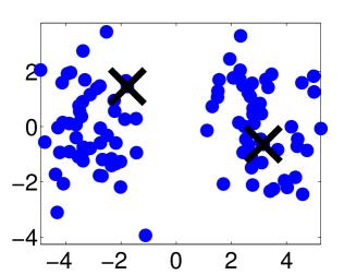
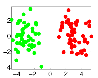
(a) (b)

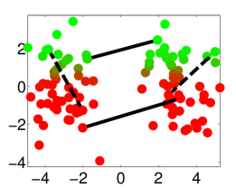
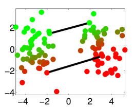
(c) (d) (e)

Figure 3: Application-specific model synthetic data: (a) Original data with initial two means marked by x. Results are represented as follows: (b) GMM, (c) GM-PR using two must-links (solid line) and two cannot-links (dashed line), (d) GM-PR using only two must-links, and (e) GM-PR using only two cannot-links. The saturation of the red/green points represents the value of the soft label.

4.2.2 UCI Repository and Handwritten Digits

In this section, we report the performance of three real datasets: 1) the Haberman’s survival dataset contains 306 instances, 3 attributes, and 2 classes; 2) the MNIST database contains images of handwritten digits. We used the test dataset, which contains 10000 examples, 784 attributes, and 10 classes [27]; and 3) the Thyroid dataset contains 215 instances, 5 attributes, and 2 classes.

We demonstrate the performance of GM-PR on two binary clustering tasks, Haberman and Thyroid, and two multiclass problems, digits 1, 2, 3 and 4, 5, 6, 7. For ease of visualization, we work with only the leading two principal components of the MNIST using principal component analysis (PCA). Figure 5 shows two-dimensional inputs, color-coded by class label. Figure 4 shows that GM-PR significantly outperforms GMM-EC regardless of the available number of links on all datasets. Moreover, Figure 6 shows that GM-PR performs well even if only the must-links are available. Compared to EM-PC, which uses only the cannot-links, Figure 7 shows the performance of GM-PR is always greater than or comparable to EM-PC and GM-PR. Figure 7 also shows that the performance of EM-PC decreases when the number of classes increases. The cannot-link in the GM-PR, on the other hand, can contribute to the model when the problem is either binary or multiclass. Notice that all the experiments indicate that GM-PR has a lower variance over 100 random initializations, which implies GM-PR stability regardless of the number of available pairwise links.

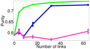
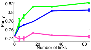
(a) Harberman (b) Thyroid

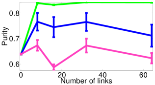
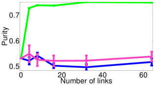
(c) digit 1, 2, and 3 (d) digit 4, 5, 6, and 7

Figure 4: The performance of GM-PR compared to GMM-EC [38] with a different number of pairwise links on (a) Harberman, (b) Thyroid, (c) digits 1, 2, and 3, and (d) digits 4, 5, 6, and 7.

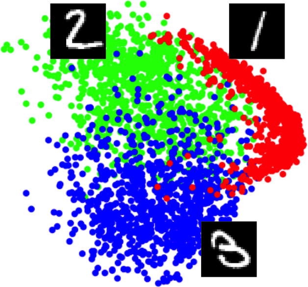
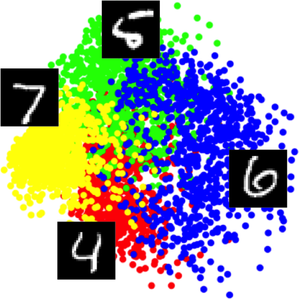
(a) digits 1, 2, and 3 (b) digits 4, 5, 6, and 7

Figure 5: Digits 1, 2, and 3, and digits 4, 5, 6, and 7 visualized by the first two principal components of PCA.

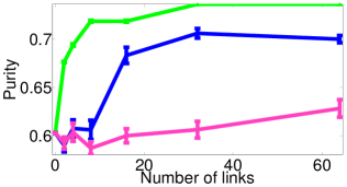
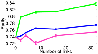
(a) Harberman used only must-links (b) Thyroid used only must-links

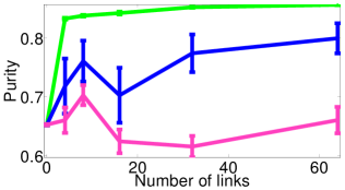
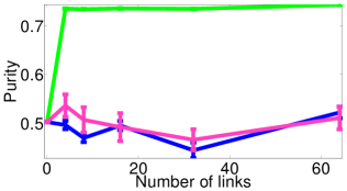
(c) digits 1, 2, and 3 (d) digits 4, 5, 6, and 7

Figure 6: The performance of GM-PR compared to GMM-EC [38] with a different number of must-links on (a) Harberman, (b) Thyroid, (c) digits 1, 2, and 3, and (d) digits 4, 5, 6, and 7.

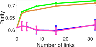
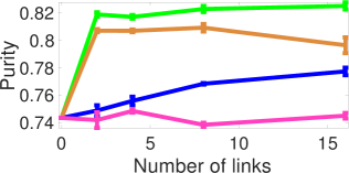
(a) Harberman (b) Thyroid

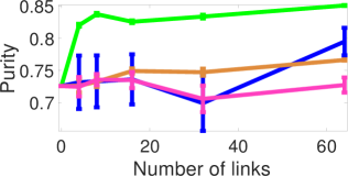
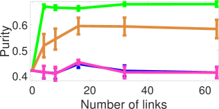
(c) digits 1, 2, and 3 (d) digits 4, 5, 6, and 7

Figure 7: The performance of GM-PR compared to GMM-EC [38] and EM-PC [20] with a different number of cannot-links on (a) Harberman, (b) Thyroid, (c) digits 1, 2, and 3, and (d) digits 4, 5, 6, and 7.

4.3 Results: Mixture of Gaussians ($m_{K}>1$)

In this section, we demonstrate the performance of the proposed model using a mixture of Gaussians on the datasets that have local manifold structure.

4.3.1 Synthetic Data: Two Moons Dataset

Data points in two moons are on a moon-like manifold structure (Figure 8(a)), which allows us to show the advantage of the proposed method using a mixture of Gaussians as a distribution instead of a single Gaussian distribution. Figure 8(a) shows the data with initial means for the GMM and the GM-PR using a single Gaussian. Figure 8(b) shows the data with initial means for GM-PR using a mixture of Gaussians ($m_{K}=2$). Figure 8(c) is the clustering result obtained from the unconstrained GMM, in which three points were assigned to the wrong class. Figure 8(c) also shows that the performance of the GMM relied on the parameter initialization. Figure 8(d) shows that the proposed GM-PR, which used a single cluster for each class, tried to learn the manifold structure via two must-link and two cannot-link relations. However, two points were still assigned to the incorrect class. Figure 8(e) shows that the GM-PR can trace the manifold structure but used the same links in (d) with two clusters for each class. This experiment illustrates the advantage of the proposed model with a mixture of distributions that traces the local data structure by every single cluster and describes the global data structure using the mixture of clusters.

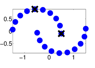
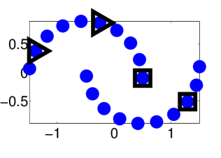
(a) (b)

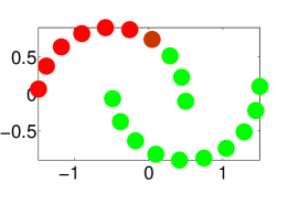
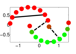
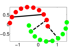
(c) (d) (e)

Figure 8: Two moons synthetic data: (a) Original data with initial two means marked by x. (b) Original data with initial means marked by triangles for class 1 and squares for class 2. Results are represented as follows: (c) GMM, (d) GM-PR used one cluster for each class, and two must-links (solid line) and two cannot-links (dashed line), and (e) GM-PR used two clusters for each class and used the same links as in (d).

4.3.2 COIL 20

In this section, we report the performance of COIL 20 datasets, which contain images of 20 objects in which each object was placed on a turntable and rotated 360 degrees to be captured with different poses via a fixed camera (Figure 9). The COIL 20 dataset contains 1440 instances and 1024 attributes. We set the number of multiclusters per class by cross-validation to $m_{K}=3$. Previous studies have shown that the intrinsic dimension of many high-dimensional real-world datasets is often quite small ($d\leq 20$) [36, 14]; therefore, each image is first projected onto the low-dimensional subspace (d = 10, 15, and 20). Figure 9 shows that the GM-PR provides higher purity values compared to the SSKK and the CSC with fewer links ($\leq 1000$) regardless of the subspace dimension. In these experiments, we found that the proposed model can outperform the graph-based method with fewer links.

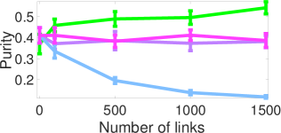
(a) d = 10 (b) d = 15

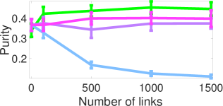
(c) d = 20 COIL-20

Figure 9: The performance of GM-PR compared to SSKK [23] and CSC [44] with a different number of cannot-links on COIL-20 (d), which are projected onto the low-dimensional subspace: (a) d = 10 (b) d = 15, and (c) d = 20.

4.4 Result: Sensitivity to Number of Clusters Per Class

Lastly, we demonstrated the performance of the proposed model in regard to different values of $m_{K}$. First, we used the same dataset (MNIST) that is used in section 4.2.2. In Figure 5(a), we observed digit 1, which clearly lay on a moon-like structure. Therefore, Figure 10(a) shows that the performance of $m_{K}=2,3$, or $4$ is better than $m_{K}=1$ when the number of links is greater than 64. However, in Figure 5(b), we observe hardly any manifold structure for digits 4, 5, 6, and 7. This observation also applies to the results in Figure 10(b). The performances of $m_{K}=1,2,3$, and $4$ are very similar to each other, e.g., increasing the value of $m_{K}$ does not help. However, we also notice that the increase in the number of $m_{K}$ does not hurt the performance of the model and might even enhance the performance depending on the dataset.

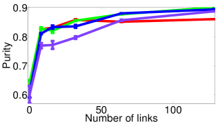
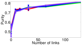
(a) digits 1, 2, and 3 (b) digits 4, 5, 6, and 7

Figure 10: The performance of GM-PR uses different values of $m_{K}$ on (a) digits 1, 2, and 3 and (b) digits 4, 5, 6, and 7.

Appendix A. Mixture of Distributions

Likelihood: Must-link Relationships

The likelihood of the $\mathcal{S}(\cdot)$ is

$$\mathcal{S}(\mathcal{X},\mathcal{Y},\mathcal{Z},\mathcal{M}, \boldsymbol{\vartheta}):=p(\mathcal{X},\mathcal{Y},\mathcal{Z}|\mathcal{M},\boldsymbol{\vartheta})=\prod_{m=1}^{M}\prod_{m_{k}=1}^{m_{K}}\prod_{(i,j)\in\mathcal{M}}\bigg{[}$$

$$\alpha_{m}\Big{[}\pi_{m_{k}}\mathcal{N}(\mathbf{x}_{i}|\boldsymbol{\mu}_{m_{k}},\boldsymbol{\Sigma}_{m_{k}})\Big{]}^{y_{i}^{m_{k}}}\Big{[}\pi_{m_{k}}\mathcal{N}(\mathbf{x}_{j}|\boldsymbol{\mu}_{m_{k}},\boldsymbol{\Sigma}_{m_{k}})\Big{]}^{y_{j}^{m_{k}}}\bigg{]}^{z_{\{ij\}}^{m}}.$$ (24)

Likelihood: Cannot-link Relationships

The likelihood of the $\mathcal{D}(\cdot)$ is

$$p(z_{a}^{m},z_{b}^{m}) = p(z_{a}^{m}|z_{b}^{m})p(z_{b}^{m}):=p(z_{b}^{m}|z_{a}^{m})p(z_{a}^{m})~{}~{}$$ (25)

$$= \left\{\begin{array}[]{ll}\cfrac{(\alpha_{m})^{z_{a}^{m}}(\alpha_{m})^{z_{b}^{m}}}{1-\sum_{m^{\prime}=1}^{M}\alpha_{m^{\prime}}^{2}}&z_{a}^{m}\neq z_{b}^{m}\\ 0&z_{a}^{m}=z_{b}^{m}\\ \end{array}\right..$$ (28)

and

$$\mathcal{D}(\mathcal{X},\mathcal{Y},\mathcal{Z},\mathcal{C},\boldsymbol{\vartheta}):=p(\mathcal{X},\mathcal{Y},\mathcal{Z}|\mathcal{C},\boldsymbol{\vartheta})=\prod_{m=1}^{M}\prod_{m_{k}=1}^{m_{K}}\prod_{(a,b)\in\mathcal{C}}$$

$$\Big{[}\pi_{m_{k}}\mathcal{N}(\mathbf{x}_{a}|\boldsymbol{\mu}_{m_{k}},\boldsymbol{\Sigma}_{m_{k}})\Big{]}^{z_{a}^{m}~{}y_{a}^{m_{k}}}\Big{[}\pi_{m_{k}}\mathcal{N}(\mathbf{x}_{b}|\boldsymbol{\mu}_{m_{k}},\boldsymbol{\Sigma}_{m_{k}})\Big{]}^{z_{b}^{m}~{}y_{b}^{m_{k}}}p(z_{a}^{m},z_{b}^{m}).$$ (29)

E-Step:

Unsupervised Scenario

The expatiation $\mathcal{L}(\cdot)$ is

$$\mathbb{E}_{z_{n}^{m},y_{n}^{m_{k}}|\mathbf{x}_{n}}[z_{n}^{m}~{}y_{n}^{m_{k}}] =p(z_{n}^{m},y_{n}^{m_{k}}|\mathbf{x}_{n})$$ (30)

$$=\frac{\alpha_{m}\pi_{m_{k}}\mathcal{N}(\mathbf{x}_{n}|\boldsymbol{\mu}_{m_{k}},\boldsymbol{\Sigma}_{m_{k}})}{\sum_{m^{\prime}=1}^{M}\sum_{m_{k}^{\prime}=1}^{m_{K}}\alpha_{m^{\prime}}\pi_{m_{k}^{\prime}}\mathcal{N}(\mathbf{x}_{n}|\boldsymbol{\mu}_{m_{k}^{\prime}},\boldsymbol{\Sigma}_{m_{k}^{\prime}})},$$

and

$$\mathbb{E}_{z_{n}^{m}|\mathbf{x}_{n}}[z_{n}^{m}] =p(z_{n}^{m}|\mathbf{x}_{n})$$

$$=\frac{\alpha_{m}\sum_{m_{k}=1}^{m_{K}}\pi_{m_{k}}\mathcal{N}(\mathbf{x}_{n}|\boldsymbol{\mu}_{m_{k}},\boldsymbol{\Sigma}_{m_{k}})}{\sum_{m^{\prime}=1}^{M}\sum_{m_{k}^{\prime}=1}^{m_{K}}\alpha_{m^{\prime}}\pi_{m_{k}^{\prime}}\mathcal{N}(\mathbf{x}_{n}|\boldsymbol{\mu}_{m_{k}^{\prime}}\boldsymbol{\Sigma}_{m_{k}^{\prime}})}.$$ (31)

Must-link Scenario

The $\mathcal{S}(\cdot)$ is

$$\mathbb{E}_{z^{m}_{\{ij\}},y_{i}^{m_{k}}|\mathbf{x}_{i},\mathbf{x}_{j}}[z^{m}_{\{ij\}}y_{i}^{m_{k}}]=p(z^{m}_{\{ij\}},y_{i}^{m_{k}}|\mathbf{x}_{i},\mathbf{x}_{j})$$

$$=\frac{\alpha_{m}\pi_{m_{k}}\mathcal{N}(\mathbf{x}_{i}|\boldsymbol{\mu}_{m_{k}},\boldsymbol{\Sigma}_{m_{k}})\sum_{m_{k^{\prime}}=1}^{m_{K}}\pi_{m_{k^{\prime}}}\mathcal{N}(\mathbf{x}_{i}|\boldsymbol{\mu}_{m_{k^{\prime}}},\boldsymbol{\Sigma}_{m_{k^{\prime}}})}{Z_{\mathcal{S}}},$$ (32)

and

$$\mathbb{E}_{z^{m}_{\{ij\}}|\mathbf{x}_{i},\mathbf{x}_{j}}[z^{m}_{\{ij\}}]=p(z^{m}_{\{ij\}}|\mathbf{x}_{i},\mathbf{x}_{j})$$

$$=\frac{\alpha_{m}\sum_{m_{k}=1}^{m_{K}}\sum_{m_{k^{\prime}}=1}^{m_{K}}\pi_{m_{k}}\pi_{m_{k^{\prime}}}\mathcal{N}(\mathbf{x}_{i}|\boldsymbol{\mu}_{m_{k}},\boldsymbol{\Sigma}_{m_{k}})\mathcal{N}(\mathbf{x}_{j}|\boldsymbol{\mu}_{m_{k^{\prime}}},\boldsymbol{\Sigma}_{m_{k^{\prime}}})}{Z_{\mathcal{S}}},$$ (33)

where

$$Z_{\mathcal{S}}=\sum_{m^{\prime}=1}^{M}\sum_{{m^{\prime}}_{k}=1}^{m_{K}}\sum_{{m^{\prime}}_{k^{\prime}}=1}^{m_{K}}\alpha_{m^{\prime}}\pi_{{m^{\prime}}_{k}}\pi_{{m^{\prime}}_{k^{\prime}}}\mathcal{N}(\mathbf{x}_{i}|\boldsymbol{\mu}_{{m^{\prime}}_{k}},\boldsymbol{\Sigma}_{{m^{\prime}}_{k}})\mathcal{N}(\mathbf{x}_{j}|\boldsymbol{\mu}_{{m^{\prime}}_{k^{\prime}}},\boldsymbol{\Sigma}_{{m^{\prime}}_{k^{\prime}}}).$$ (34)

Cannot-link Scenario

The $\mathcal{D}(\cdot)$ is

$$\mathbb{E}_{z^{m}_{a},y_{a}^{m_{k}}|\mathbf{x}_{a},\mathbf{x}_{b}}[z_{a}^{m}~{}y_{a}^{m_{k}}]=p(z_{a}^{m},y_{a}^{m_{k}}|\mathbf{x}_{a},\mathbf{x}_{b})=$$

$$\frac{\pi_{m_{k}}\mathcal{N}(\mathbf{x}_{a}|\boldsymbol{\mu}_{m_{k}},\boldsymbol{\Sigma}_{m_{k}})\sum_{m^{\prime}=1}^{M}\sum_{{m^{\prime}}_{k}=1}^{m_{K}}\pi_{{m^{\prime}}_{k}}\mathcal{N}(\mathbf{x}_{b}|\boldsymbol{\mu}_{{m^{\prime}}_{k}},\boldsymbol{\Sigma}_{{m^{\prime}}_{k}})p(z_{a}^{m},z_{b}^{m^{\prime}})}{Z_{\mathcal{D}}},$$ (35)

and

$$\mathbb{E}_{z^{m}_{a}|\mathbf{x}_{a},\mathbf{x}_{b}}[z_{a}^{m}]=p(z_{a}^{m}|\mathbf{x}_{a},\mathbf{x}_{b})=$$

$$\frac{\begin{multlined}\sum_{m_{k}=1}^{m_{K}}\pi_{m_{k}}\mathcal{N}(\mathbf{x}_{a}|\boldsymbol{\mu}_{m_{k}},\boldsymbol{\Sigma}_{m_{k}})\sum_{m^{\prime}=1}^{M}\sum_{{m^{\prime}}_{k}=1}^{m_{K}}\pi_{{m^{\prime}}_{k}}\mathcal{N}(\mathbf{x}_{b}|\boldsymbol{\mu}_{{m^{\prime}}_{k}},\boldsymbol{\Sigma}_{{m^{\prime}}_{k}})\\ p(z_{a}^{m},z_{b}^{m^{\prime}})\end{multlined}\sum_{m_{k}=1}^{m_{K}}\pi_{m_{k}}\mathcal{N}(\mathbf{x}_{a}|\boldsymbol{\mu}_{m_{k}},\boldsymbol{\Sigma}_{m_{k}})\sum_{m^{\prime}=1}^{M}\sum_{{m^{\prime}}_{k}=1}^{m_{K}}\pi_{{m^{\prime}}_{k}}\mathcal{N}(\mathbf{x}_{b}|\boldsymbol{\mu}_{{m^{\prime}}_{k}},\boldsymbol{\Sigma}_{{m^{\prime}}_{k}})\\ p(z_{a}^{m},z_{b}^{m^{\prime}})}{Z_{\mathcal{D}}},$$ (38)

where

$$Z_{\mathcal{D}}=\sum_{m^{\prime\prime}=1}^{M}\sum_{m^{\prime\prime\prime}=1}^{M}\sum_{{m^{\prime\prime}}_{k}=1}^{m_{K}}\sum_{{m^{\prime\prime\prime}}_{k}=1}^{m_{K}}\pi_{{m^{\prime\prime}}_{k}}\pi_{{m^{\prime\prime\prime}}_{k}} \mathcal{N}(\mathbf{x}_{a}|\boldsymbol{\mu}_{{m^{\prime\prime}}_{k}},\boldsymbol{\Sigma}_{{m^{\prime\prime}}_{k}})$$

$$\mathcal{N}(\mathbf{x}_{b}|\boldsymbol{\mu}_{{m^{\prime\prime\prime}}_{k}},\boldsymbol{\Sigma}_{{m^{\prime\prime\prime}}_{k}})p(z_{a}^{m^{\prime\prime}},z_{b}^{m^{\prime\prime\prime}}).$$ (39)

M-Step

The mean and covariance in the $k$th cluster in the $m$th class are

$$\boldsymbol{\mu}_{m_{k}}=\frac{\sum_{n}\ell_{n}^{m_{k}}\mathbf{x}_{n}+\sum_{(i,j)\in\mathcal{M}}\big{[}s_{i}^{m_{k}}\mathbf{x}_{i}+s_{j}^{m_{k}}\mathbf{x}_{j}\big{]}+\sum_{(a,b)\in\mathcal{C}}\big{[}d_{a}^{m_{k}}\mathbf{x}_{a}+d_{b}^{m_{k}}\mathbf{x}_{b}\big{]}}{\sum_{n}\ell_{n}^{m_{k}}+\sum_{(i,j)\in\mathcal{M}}\big{[}s_{i}^{m_{k}}+s_{j}^{m_{k}}\big{]}+\sum_{(a,b)\in\mathcal{C}}\big{[}d_{a}^{m_{k}}+d_{b}^{m_{k}}\big{]}},$$ (40)

$$\boldsymbol{\Sigma}_{m_{k}}=\frac{\begin{multlined}\sum_{n}\ell_{n}^{m_{k}}\mathbf{S}_{n}^{m_{k}}+\sum_{(i,j)\in\mathcal{M}}\big{[}s_{i}^{m_{k}}\mathbf{S}_{i}^{m_{k}}+s_{j}^{m_{k}}\mathbf{S}_{j}^{m_{k}}\big{]}+\sum_{(a,b)\in\mathcal{C}}\big{[}\\ d_{a}^{m_{k}}\mathbf{S}_{a}^{m_{k}}+d_{b}^{m_{k}}\mathbf{S}_{b}^{m_{k}}\big{]}\end{multlined}\sum_{n}\ell_{n}^{m_{k}}\mathbf{S}_{n}^{m_{k}}+\sum_{(i,j)\in\mathcal{M}}\big{[}s_{i}^{m_{k}}\mathbf{S}_{i}^{m_{k}}+s_{j}^{m_{k}}\mathbf{S}_{j}^{m_{k}}\big{]}+\sum_{(a,b)\in\mathcal{C}}\big{[}\\ d_{a}^{m_{k}}\mathbf{S}_{a}^{m_{k}}+d_{b}^{m_{k}}\mathbf{S}_{b}^{m_{k}}\big{]}}{\sum_{n}\ell_{n}^{m_{k}}+\sum_{(i,j)\in\mathcal{M}}\big{[}s_{i}^{m_{k}}+s_{j}^{m_{k}}\big{]}+\sum_{(a,b)\in\mathcal{C}}\big{[}d_{a}^{m_{k}}+d_{b}^{m_{k}}\big{]}},$$ (43)

where

$$\ell_{n}^{m_{k}} =p(z_{n}^{m},y_{n}^{m_{k}}|\mathbf{x}_{n}),$$

$$s_{i}^{m_{k}} =p(z_{\{ij\}}^{m},y_{i}^{m_{k}}|\mathbf{x}_{i},\mathbf{x}_{j}),$$

$$d_{a}^{m_{k}} =p(z_{a}^{m},y_{a}^{m_{k}}|\mathbf{x}_{a},\mathbf{x}_{b}),$$ (44)

and

$$\mathbf{S}_{n}^{m_{k}}=(\mathbf{x}_{n}-\boldsymbol{\mu}_{m_{k}})(\mathbf{x}_{n}-\boldsymbol{\mu}_{m_{k}})^{T}.$$ (45)

Because the mixing parameter for the cluster $\pi_{m_{k}}$ satisfies the summation to one, the determination can be achieved by the Lagrange multiplier.

$$\mathcal{Q}_{\mathcal{J}}+\lambda\bigg{(}\sum_{m_{k}=1}^{m_{K}}\pi_{m_{k}}-1\bigg{)}$$ (46)

$\lambda$ is the Lagrange multiplier. Taking the derivative of equation (46) with respect to $\pi_{m_{k}}$,

$$\frac{\sum_{n=1}^{N}\ell_{n}^{m_{k}}+\sum_{(i,j)\in\mathcal{M}}\big{[}s_{i}^{m_{k}}+s_{j}^{m_{k}}\big{]}+\sum_{(a,b)\in\mathcal{C}}\big{[}d_{a}^{m_{k}}+d_{b}^{m_{k}}\big{]}}{\pi_{m_{k}}}+\lambda=0$$ (47)

By taking the derivative of equation (46) with respect to $\lambda$ and equal to zero, we then can get $\sum_{m_{k}=1}^{m_{K}}\pi_{m_{k}}=1$ and use it to eliminate the $\lambda$ in equation (47). The mixing parameter for the $k$th cluster in the $m$th mixture is given by

$$\pi_{m_{k}}=\frac{\sum_{n=1}^{N}\ell_{n}^{m_{k}}+\sum_{(i,j)\in\mathcal{M}}\big{[}s_{i}^{m_{k}}+s_{j}^{m_{k}}\big{]}+\sum_{(a,b)\in\mathcal{C}}\big{[}d_{a}^{m_{k}}+d_{b}^{m_{k}}\big{]}}{\sum_{m_{k}=1}^{m_{K}}\Big{(}\sum_{n=1}^{N}\ell_{n}^{m_{k}}+\sum_{(i,j)\in\mathcal{M}}\big{[}s_{i}^{m_{k}}+s_{j}^{m_{k}}\big{]}+\sum_{(a,b)\in\mathcal{C}}\big{[}d_{a}^{m_{k}}+d_{b}^{m_{k}}\big{]}\Big{)}}$$ (48)

Lastly, estimating the mixing parameters for mixture $\alpha_{m}$ is the same as in equation (3.4).

References

- [1] Abramowitz, M., Stegun, I.A.: Handbook of mathematical functions: with formulas, graphs, and mathematical tables, vol. 55. Courier Corporation (1964)
- [2] Allab, K., Benabdeslem, K.: Constraint selection for semi-supervised topological clustering. In: Machine Learning and Knowledge Discovery in Databases, pp. 28–43. Springer (2011)
- [3] Arthur, D., Vassilvitskii, S.: k-means++: The advantages of careful seeding. In: Proceedings of the eighteenth annual ACM-SIAM symposium on Discrete algorithms, pp. 1027–1035. Society for Industrial and Applied Mathematics (2007)
- [4] Bar-Hillel, A., Hertz, T., Shental, N., Weinshall, D.: Learning a mahalanobis metric from equivalence constraints. Journal of Machine Learning Research 6(6), 937–965 (2005)
- [5] Basu, S., Bilenko, M., Mooney, R.J.: A probabilistic framework for semi-supervised clustering. In: Proceedings of the tenth ACM SIGKDD international conference on Knowledge discovery and data mining, pp. 59–68. ACM (2004)
- [6] Basu, S., Davidson, I., Wagstaff, K.: Constrained clustering: Advances in algorithms, theory, and applications. CRC Press (2008)
- [7] Chapelle, O., Schölkopf, B., Zien, A., et al.: Semi-supervised learning, vol. 2. MIT press Cambridge (2006)
- [8] Cohn, D., Caruana, R., McCallum, A.: Semi-supervised clustering with user feedback. Constrained Clustering: Advances in Algorithms, Theory, and Applications 4(1), 17–32 (2003)
- [9] Coviello, E., Lanckriet, G.R., Chan, A.B.: The variational hierarchical em algorithm for clustering hidden markov models. In: Advances in neural information processing systems, pp. 404–412 (2012)
- [10] Cozman, F.G., Cohen, I., Cirelo, M.C., et al.: Semi-supervised learning of mixture models. In: international conference on Machine learning, pp. 99–106 (2003)
- [11] Dara, R., Kremer, S.C., Stacey, D., et al.: Clustering unlabeled data with soms improves classification of labeled real-world data. In: Neural Networks, 2002. IJCNN’02. Proceedings of the 2002 International Joint Conference on, vol. 3, pp. 2237–2242. IEEE (2002)
- [12] Demiriz, A., Bennett, K.P., Embrechts, M.J.: Semi-supervised clustering using genetic algorithms. Artificial neural networks in engineering (ANNIE-99) pp. 809–814 (1999)
- [13] Dempster, A.P., Laird, N.M., Rubin, D.B.: Maximum likelihood from incomplete data via the em algorithm. Journal of the Royal Statistical Society. Series B (Methodological) pp. 1–38 (1977)
- [14] Felsberg, M., Kalkan, S., Krüger, N.: Continuous dimensionality characterization of image structures. Image and Vision Computing 27(6), 628–636 (2009)
- [15] Fletcher, R.: Practical methods of optimization. John Wiley & Sons (2013)
- [16] Gammerman, A., Vovk, V., Vapnik, V.: Learning by transduction. In: Proceedings of the Fourteenth conference on Uncertainty in artificial intelligence, pp. 148–155. Morgan Kaufmann Publishers Inc. (1998)
- [17] Goldberg, A.B., Zhu, X., Singh, A., Xu, Z., Nowak, R.: Multi-manifold semi-supervised learning (2009)
- [18] Goldberger, J., Roweis, S.T.: Hierarchical clustering of a mixture model. In: Advances in Neural Information Processing Systems, pp. 505–512 (2004)
- [19] Gonzalez, T.F.: Clustering to minimize the maximum intercluster distance. Theoretical Computer Science 38, 293–306 (1985)
- [20] Graca, J., Ganchev, K., Taskar, B.: Expectation maximization and posterior constraints. In: Advances in neural information processing systems (2007)
- [21] He, X., Cai, D., Shao, Y., Bao, H., Han, J.: Laplacian regularized gaussian mixture model for data clustering. Knowledge and Data Engineering, IEEE Transactions on 23(9), 1406–1418 (2011)
- [22] Jordan, M.I., Jacobs, R.A.: Hierarchical mixtures of experts and the em algorithm. Neural computation 6(2), 181–214 (1994)
- [23] Kulis, B., Basu, S., Dhillon, I., Mooney, R.: Semi-supervised graph clustering: a kernel approach. Machine Learning 74(1), 1–22 (2009)
- [24] Kyriakopoulou, A., Kalamboukis, T.: The impact of semi-supervised clustering on text classification. In: Proceedings of the 17th Panhellenic Conference on Informatics, pp. 180–187. ACM (2013)
- [25] Law, M.H., Topchy, A.P., Jain, A.K.: Model-based clustering with probabilistic constraints. In: SDM, pp. 641–645. SIAM (2005)
- [26] Le Nguyen, M., Shimazu, A.: A semi supervised learning model for mapping sentences to logical forms with ambiguous supervision. Data & Knowledge Engineering 90, 1–12 (2014)
- [27] LeCun, Y., Bottou, L., Bengio, Y., Haffner, P.: Gradient-based learning applied to document recognition. Proceedings of the IEEE 86(11), 2278–2324 (1998)
- [28] Liu, J., Cai, D., He, X.: Gaussian mixture model with local consistency. In: AAAI, vol. 10, pp. 512–517. Citeseer (2010)
- [29] Loog, M.: Semi-supervised linear discriminant analysis through moment-constraint parameter estimation. Pattern Recognition Letters 37, 24–31 (2014)
- [30] Lu, Z., Leen, T.K.: Semi-supervised learning with penalized probabilistic clustering. In: Advances in neural information processing systems, pp. 849–856 (2004)
- [31] Mann, G.S., McCallum, A.: Generalized expectation criteria for semi-supervised learning with weakly labeled data. The Journal of Machine Learning Research 11, 955–984 (2010)
- [32] Manning, C.D., Raghavan, P., Schütze, H.: Introduction to information retrieval, vol. 1. Cambridge university press Cambridge (2008)
- [33] Meila, M., Jordan, M.I.: Learning with mixtures of trees. The Journal of Machine Learning Research 1, 1–48 (2001)
- [34] Nguyen, T.P., Ho, T.B.: Detecting disease genes based on semi-supervised learning and protein–protein interaction networks. Artificial intelligence in medicine 54(1), 63–71 (2012)
- [35] Nigam, K., McCallum, A.K., Thrun, S., Mitchell, T.: Text classification from labeled and unlabeled documents using em. Machine learning 39(2-3), 103–134 (2000)
- [36] Raginsky, M., Lazebnik, S.: Estimation of intrinsic dimensionality using high-rate vector quantization. In: Advances in neural information processing systems, pp. 1105–1112 (2005)
- [37] Shen, J., Bu, J., Ju, B., Jiang, T., Wu, H., Li, L.: Refining gaussian mixture model based on enhanced manifold learning. Neurocomputing 87, 19–25 (2012)
- [38] Shental, N., Bar-Hillel, A., Hertz, T., Weinshall, D.: Computing gaussian mixture models with em using equivalence constraints. Advances in neural information processing systems 16(8), 465–472 (2004)
- [39] Singh, A., Nowak, R., Zhu, X.: Unlabeled data: Now it helps, now it doesn’t. In: Advances in neural information processing systems, pp. 1513–1520 (2009)
- [40] Sirts, K., Goldwater, S.: Minimally-supervised morphological segmentation using adaptor grammars. Transactions of the Association for Computational Linguistics 1, 255–266 (2013)
- [41] Titsias, M.K., Likas, A.: Mixture of experts classification using a hierarchical mixture model. Neural Computation 14(9), 2221–2244 (2002)
- [42] Vasconcelos, N., Lippman, A.: Learning mixture hierarchies. In: NIPS, pp. 606–612. Citeseer (1998)
- [43] Wagstaff, K., Cardie, C., Rogers, S., Schrödl, S., et al.: Constrained k-means clustering with background knowledge. In: international conference on Machine learning, vol. 1, pp. 577–584 (2001)
- [44] Wang, X., Davidson, I.: Flexible constrained spectral clustering. In: Proceedings of the 16th ACM SIGKDD international conference on Knowledge discovery and data mining, pp. 563–572. ACM (2010)
- [45] Weinberger, K.Q., Blitzer, J., Saul, L.K.: Distance metric learning for large margin nearest neighbor classification. In: Advances in neural information processing systems, pp. 1473–1480 (2005)
- [46] Williams, C.K.: A mcmc approach to hierarchical mixture modelling. In: NIPS, pp. 680–686. Citeseer (1999)
- [47] Xing, E.P., Jordan, M.I., Russell, S., Ng, A.Y.: Distance metric learning with application to clustering with side-information. In: Advances in neural information processing systems, pp. 505–512 (2002)
- [48] Xing, X., Yu, Y., Jiang, H., Du, S.: A multi-manifold semi-supervised gaussian mixture model for pattern classification. Pattern Recognition Letters 34(16), 2118–2125 (2013)
- [49] Xiong, C., Johnson, D., Corso, J.J.: Spectral active clustering via purification of the k-nearest neighbor graph. In: Proc. of European Conference on Data Mining (2012)
- [50] Yang, T., Priebe, C.E.: The effect of model misspecification on semi-supervised classification. Pattern Analysis and Machine Intelligence, IEEE Transactions on 33(10), 2093–2103 (2011)
- [51] Yang, Y., Nie, F., Xu, D., Luo, J., Zhuang, Y., Pan, Y.: A multimedia retrieval framework based on semi-supervised ranking and relevance feedback. Pattern Analysis and Machine Intelligence, IEEE Transactions on 34(4), 723–742 (2012)
- [52] Yi, J., Zhang, L., Jin, R., Qian, Q., Jain, A.: Semi-supervised clustering by input pattern assisted pairwise similarity matrix completion. In: Proceedings of the 30th International Conference on Machine Learning (ICML-13), pp. 1400–1408 (2013)
- [53] Zhu, X., Goldberg, A.B.: Introduction to semi-supervised learning. Synthesis lectures on artificial intelligence and machine learning 3(1), 1–130 (2009)
- [54] Zhu, X., Lafferty, J.: Harmonic mixtures: combining mixture models and graph-based methods for inductive and scalable semi-supervised learning. In: Proceedings of the 22nd international conference on Machine learning, pp. 1052–1059. ACM (2005)