Chemical composition of two bright extremely metal-poor stars from the
SDSS MARVELS pre-survey

Abstract

SDSS J082625.70+612515.10 (V = 11.4; [Fe/H] = $-$3.1) and SDSS J134144.60+474128.90 (V = 12.4; [Fe/H] = $-$3.2) were observed with the SDSS 2.5-m telescope as part of the SDSS-MARVELS spectroscopic pre-survey, and were identified as extremely metal-poor (EMP; [Fe/H] $<-3.0$) stars during high-resolution follow-up with the Hanle Echelle Spectrograph (HESP) on the 2.3-m Himalayan Chandra Telescope. In this paper, the first science results using HESP, we present a detailed analysis of their chemical abundances. Both stars exhibit under-abundances in their neutron-capture elements, while one of them, SDSS J134144.60+474128.90, is clearly enhanced in carbon. Lithium was also detected in this star at a level of about A(Li) = 1.95. The spectra were obtained over a span of 6-24 months, and indicate that both stars could be members of binary systems. We compare the elemental abundances derived for these two stars along with other carbon-enhanced metal-poor (CEMP) and EMP stars, in order to understand the nature of their parent supernovae. We find that CEMP-no stars and EMP dwarfs exhibit very similar trends in their lithium abundances at various metallicities. We also find indications that CEMP-no stars have larger abundances of Cr and Co at a given metallicity, compared to EMP stars.

1. Introduction

Extremely metal-poor (EMP; [Fe/H] $<-3.0$) stars of the Galactic halo are thought to be the immediate successors of the first stars, and were likely to have formed when the Universe was only a few hundred million years old (e.g., Bromm et al. 2009) – their evolution and explosion led to the first production of heavy elements. These first supernovae had a considerable dynamical, thermal, and chemical impact on the evolution of the surrounding interstellar medium, including mini-halos that can be some distance away from the location of the first-star explosion (Cooke & Madau, 2014; Smith et al., 2015; Chiaki et al., 2018). Stars (and their host galaxies) that formed thereafter are expected to carry the imprints of the nucleosynthesis events from these Population III stars (Beers & Christlieb, 2005; Frebel & Norris, 2015; Sharma et al., 2018). Studies of such EMP stars have greatly benefited from the large spectroscopic surveys that were carried out in the past in order to identify them in significant numbers, such as the HK survey of Beers and collaborators (Beers et al., 1985, 1992) and the Hamburg/ESO Survey of Christlieb and colleagues (Christlieb, 2003). More recent surveys, such as SDSS, RAVE, APOGEE and LAMOST continue to expand the known members of this rare class of stars (e.g., Fulbright et al. 2010; Ivezić et al. 2012; Aoki et al. 2013; Zhao et al. 2012; García Pérez et al. 2013; Anders et al. 2014; Li et al. 2015).

High-resolution spectroscopic studies of metal-poor Galactic halo stars have demonstrated diversity in their chemical compositions. For example, on the order of 20% of stars with [Fe/H] $<-2.0$ exhibit large enhancements in their carbon-to-iron ratios ([C/Fe] $>+0.7$; Aoki et al. 2007; Lee et al. 2013; Lee et al. 2017). As shown by numerous studies, the frequency of carbon-enhanced metal-poor (CEMP) stars continues to increase with decreasing [Fe/H]. The fractions of CEMP stars also increase with distance from the Galactic plane (Frebel et al., 2006; Beers et al., 2017), and also between the inner-halo and the outer-halo regions (Lee et al., 2017).

CEMP stars can be separated into four sub-classes (Beers & Christlieb, 2005): i) CEMP-$s$ stars, which show enhancements of $s$-process elements, ii) CEMP-$r$ stars, which exhibit enhancements of $r$-process elements, iii) CEMP-$r/s$ stars, which show enhancements in both $r$- and $s$-process elements, and iv) CEMP-no stars, which exhibit no neutron-capture element enhancements. Long-term radial-velocity monitoring studies have shown that most ($>80$%, possibly all) CEMP-$s$ stars are members of binary systems involving a (now extinct) asymptotic giant branch (AGB) star that transferred carbon and $s$-process rich material to the presently observed (lower-mass) star (Lucatello et al., 2005; Starkenburg et al., 2014; Hansen et al., 2016b), while CEMP-no stars exhibit observed binary frequencies typical of non-carbon-enhanced halo giants, $\sim 18$% (Starkenburg et al., 2014; Hansen et al., 2016a).

Yoon et al. (2016) have considered the rich morphology of the absolute abundance of carbon, $A$(C)$=log(C)$, as a function of [Fe/H], based on high-resolution analyses of a large sample of CEMP stars (their Figure 1, the Yoon-Beers diagram). In addition to their Group I stars, which are dominated by CEMP-$s$ stars, they demonstrate that the CEMP-no stars not only exhibit substantially lower $A$(C), but bifurcate into two apparently different regions of the diagram, which they refer to as Group II and Group III stars. This behavior immediately suggests that these groups might be associated with different progenitors responsible for the carbon production, a suggestion borne out by the modeling carried out by Placco et al. (2016), and/or on the masses of the mini-halos in which these stars formed. Chiaki et al. (2017) have emphasized that different cooling pathways, dependent on the formation of carbon or silicate dust, may have applied to the Group III and Group II stars in the Yoon-Beers diagram.

Multiple models for the production of CEMP-no stars have been considered in the literature, such as the “spinstar” models (e.g., Meynet et al. 2006; Meynet et al. 2010; Chiappini 2013), and the “mixing and fallback” models for faint SNe (e.g., Umeda & Nomoto 2003; Umeda & Nomoto 2005; Nomoto et al. 2013; Tominaga et al. 2014). Both processes may well play a role (Maeder & Meynet, 2015; Choplin et al., 2016).

Regardless of the complexity of the situation, additional detailed observations of EMP stars with and without clear carbon enhancement, such as those carried out here, are required for progress in understanding. This paper is outlined as follows. In Section 2 we describe our high-resolution observations. Consideration of possible radial-velocity variations for our two targets is presented in Section 3. Section 4 summarizes our estimates of stellar atmospheric parameters, and describes our abundance analyses. Results of the abundance analysis are reported in Section 5. We present a discussion of our results with a comparative study of CEMP-no and EMP stars in Section 6, along with a brief conclusion in Section 7.

2. Observations and Analysis

2.1. Sample Selection

MARVELS (Paegert et al., 2015), a multi-object radial-velocity survey designed for efficient exo-planet searches, was one of the three sub-surveys carried out as part of SDSS-III (Eisenstein et al., 2011). The targets for the first two years of MARVELS were selected based on a lower-resolution ($R\sim 1800)$ spectroscopic pre-survey using the SDSS spectrographs. Most of the pre-survey observations were carried out during twilight, when the fields were at low elevation. Targets were selected from these pre-survey fields for the MARVELS main radial velocity (RV) survey, which were later observed at higher elevations. There were about 30,000 stars observed as part of the spectroscopic pre-survey of stars with $B-V>0.6$ and $8<V<13$. Target fields for the first two years of the MARVELS survey were around known RV standards, and about 75% of the target fields were in the Galactic latitude range $2^{\circ}<|b|<30^{\circ}$. Although not the ideal location to find metal-poor stars, it does offer the chance to identify a small number of bright halo targets, suitable for high-resolution spectroscopic follow-up with moderate-aperture telescopes, that happen to fall into the MARVELS pre-survey footprint during their orbits about the Galactic center. The pre-survey also has simple magnitude and color cuts, which reduces potential selection biases. As in our previously published work (Susmitha Rani et al., 2016), we used synthetic spectral fitting of the pre-survey data to identify new metal-poor candidates. Here, we present high-resolution observations and analysis of two EMP stars, SDSS J082625.70+612515.10 (hereafter, SDSS J0826+6125) and SDSS J134144.60+474128.90 (hereafter, SDSS J1341+4741), with $V$ magnitudes of 11.44 and 12.38, respectively. These two stars were selected for follow up, as they were found to be very metal poor from spectral fitting of the pre-survey data, and were also very bright. Results from the spectral fitting used to identify metal-poor candidates from the MARVELS pre-survey will be discussed in a separate paper.

2.2. High-Resolution Observations

High-resolution ($R\sim 30,000$) spectroscopic observations of the two EMP stars were obtained with the Hanle Echelle Spectrograph (HESP) on the 2.3-m Himalayan Chandra telescope (HCT) at the Indian Astronomical Observatory (IAO). The dates of observation, wavelength coverage, radial velocities, and signal-to-noise ratios of the available spectra are listed in Tables 1 and 2.

Data reduction was carried out using the IRAF echelle package. HESP has a dual fiber mode available, one fiber for the target star and another, which can be fed with a calibration source for precise RV measurements, or by the night sky through a pinhole that has a separation of about 13″ from the target. The sky fiber is used for background subtraction. All the orders were normalized, corrected for radial velocity, and merged to produce the final spectrum. The equivalent widths for individual species are listed in the tables in the appendix. Recently, a custom data reduction pipeline has been developed by A. Surya (available publicly) that is more suitable for the crowded and curved orders of the stellar spectra observed with HESP. However, in the present paper, we use IRAF, and proper care was taken to avoid drift of the spectral tracings blending into adjacent orders.

Table 1Observation log and radial velocities for SDSS J0826+6125

Date	MJD	$\lambda$ Coverage	SNR	Radial Velocity
		(Å)		(km sec-1)
2015-11-03	57330.20903	3600-10800	51	$-$110.4
2015-11-29	57356.36042	3600-10800	49	$-$95.6
2015-12-22	57379.10417	3600-10800	47	$-$80.3
2016-01-27	57415.09792	3600-10800	47	$-$52.3
2016-10-20	57682.21667	3600-10800	50	$-$108.9
2016-11-16	57709.13542	3600-10800	51	$-$104.1

Table 2Observation log and radial velocities for SDSS J1341+4741

Date	MJD	$\lambda$ Coverage	SNR	Radial Velocity
		(Å)		(km sec-1)
2016-27-01	57415.24722	3600-10800	43	$-$240.1
2016-24-04	57503.18819	3600-1080	49	$-$190.5
2016-26-04	57505.06458	3600-1080	47	$-$192.1
2016-24-06	57564.02361	3600-1080	48	$-$176.2
2016-25-06	57565.20139	3600-1080	47	$-$174.5

3. RADIAL VELOCITIES

The HESP instrument is thermally controlled to ${\Delta}T$ = $\pm$ 0.1^∘ C at a set point of 16^∘ C over the entire year, which is expected to provide a long-term stability of $\sim 200$ m s^-1 (Sivarani et al. in preparation), substantially lowering systematic errors with respect to a spectrograph that does not have such control.

RVs were calculated for SDSS J0826+6125 based on six epochs of observations spread over a period of 12 months. For SDSS J1341+4741, we obtained five observations spread over six months. A cross-correlation analysis was performed with a synthetic template spectrum suitable for each star to obtain the RV measurement for each spectrum. We made use of the software package RVLIN provided by Wright & Howard (2009), which is a set of IDL routines used to fit Keplerian orbits to derive the orbital parameters from the RV data. The RV measurements exhibit peak-to-peak variations of $\sim 60$ km s^-1, with a period of 180 days for SDSS J0826+6125, and $\sim 110$ km s^-1, with a period of 116 days for SDSS J1341+4741. The best-fit orbits for these stars, based on the data in hand, are shown in Figures 1 and 2. Although the existence of RV variations is secure, with such sparse coverage of the proposed orbits more data are required to confirm the periods.

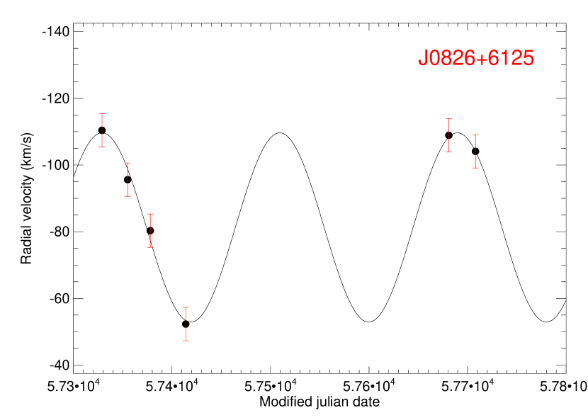
Figure 1.— Variation of radial velocity for SDSS J0826+6125. The derived period is of 180.4 days

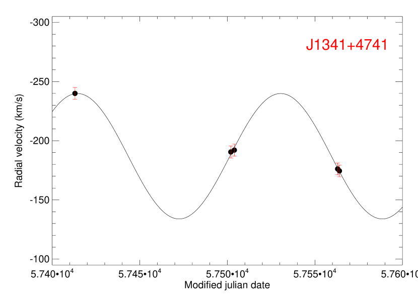
Figure 2.— Variation of radial velocity for SDSS J1341+4741. The derived period is 116.0 days

4. STELLAR PARAMETERS

Both photometric and spectroscopic data were used to derive estimates of the stellar parameters for our program stars. The effective temperatures were determined using various photometric observations in the literature and the $T_{\rm eff}$-color relations derived by Ramírez & Meléndez (2005). They were found to be in close proximity (a difference of   40 K was found) to values obtained using Alonso et al. (1996) and Alonso et al. (1999). The $V-K$ temperature estimate is expected to be superior, as it is least affected by metallicity and the possible presence of molecular carbon bands. We also employed VOSA (http://svo2.cab.inta-csic.es/), the online SED fitter (Bayo et al., 2008), to derive the temperatures using all of the available photometry (optical, 2MASS, and WISE). A Bayesian fit using the Kurucz ODFNEW/NOVER model was used to obtain the SED temperature. Final fits for the two stars are shown in Figures 3 and 4.

$T_{\rm eff}$ estimates have also been derived spectroscopically, by demanding that there be no trend of Fe I line abundances with excitation potential (shown in the upper panels of Figures 5 and 6), as well by fitting the $H_{\alpha}$ profiles. Estimates for the effective temperatures of our target stars are listed in Table 3.  For SDSS J1341+4741,   we have adopted the temperature obtained from fitting of the $H_{\alpha}$  wings, as it is highly sensitive to small variations in temperature. For SDSS J0826+6125, the $H_{\alpha}$  profile was asymmetric, and thus it could not be used for accurate measurement of temperature. So, the temperature obtained from Fe I line abundances was adopted.

Surface gravity, $\log(g)$, estimates for the two stars have been determined by the usual technique that demands equality of the iron abundances derived for the neutral (Fe I) lines and singly ionized (Fe II) lines. We used 7 Fe II lines and 82 Fe I lines for SDSS J0826+6125, and 5 Fe II lines and 49 Fe I lines for SDSS J1341+4741; best-fit models for our target stars are shown in the upper panels of Figures 5 and 6. The wings of the Mg I lines have also been fitted to obtain estimates for $\log(g)$; best-fit models are shown in Figure 7.

The microturbulent velocity ($\xi$) estimates for each star have been derived iteratively in this process, by demanding no trend of Fe I abundances with the reduced equivalent widths, and are plotted in the lower panels of figures 5 and 6. The final adopted stellar atmospheric parameters are listed in Table 4.

Table 3Estimates of Effective Temperature

Method	$T_{\rm eff}$ (K)
	SDSS J0826+6125	SDSS J1341+4741
$V-K$	4453	5827
SED	4500	5500
H$\alpha$	4400	5450
Fe I/Fe II	4300	5400

Table 4Adopted Stellar Parameters

Object	$T_{\rm eff}$ (K)	$\log(g)$	$\xi$	[Fe$/$H]
SDSS J0826+6125	4300	0.40	1.80	$-$3.10
SDSS J1341+4741	5450	2.50	1.80	$-$3.20

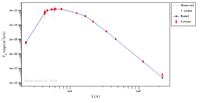
Figure 3.— The SED obtained from VOSA for SDSS J0826+6125 shows the temperature to be $\sim$4500 K.

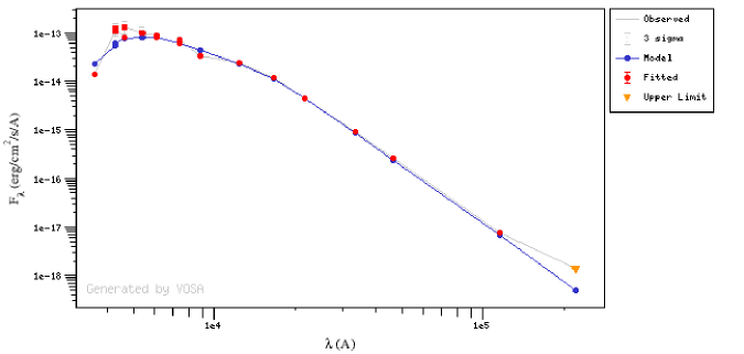
Figure 4.— The SED obtained from VOSA for SDSS J1341+4741 shows the temperature to be $\sim$5500 K.

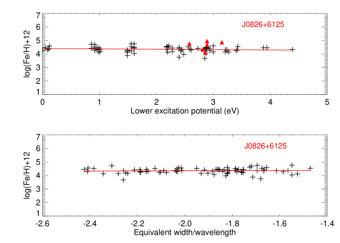
Figure 5.— Top panel: Fe abundances derived from all lines, as a function of the lower excitation potential, for the adopted model for SDSS J0826+6125. Lower panel: Fe abundances, as a function of reduced equivalent widths, for the measured lines.

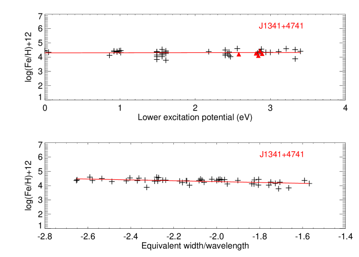
Figure 6.— Top panel: Fe abundances derived from all lines, as a function of the lower excitation potential, for the adopted model for SDSS J1341+4741. Lower panel: Fe abundances, as a function of reduced equivalent widths, for the measured lines.

Figure 7.— High-resolution HESP spectra of SDSS J0826+6125 (upper panel) and SDSS J1341+4741 (lower panel) in the region of the Mg I triplet for different values of $\log(g)$, in steps of 0.25 dex. The red solid line indicates the best-fit synthetic spectrum. The adopted paremeters for SDSS J0826+6125 are $T_{\rm eff}$ = 4300 K and $\log(g)=0.40$, while those for SDSS J1341+4741 are $T_{\rm eff}$ = 5450 K and $\log(g)$ = 2.50.

4.1. Abundance Analysis

To determine the abundance estimates for the various elements present in our target stars we have employed one dimensional LTE stellar atmospheric models (ATLAS9; Castelli & Kurucz 2004) and the spectral synthesis code turbospectrum (Alvarez & Plez, 1998). We measured the equivalent widths of the absorption lines present in the spectra, and considered only those lines for abundance analysis whose equivalent width is less than 120 mÅ, since they are on the linear part of the curve of growth, and are relatively insensitive to the choice of microturbulence. We measured the equivalent widths of 53 clean lines present in the spectra of SDSS J0826+6125, among which 82 are Fe I lines, and 122 clean lines for SDSS J1341+4741, among which 49 are Fe I lines. We have adopted the solar abundances for each element from Asplund et al. (2009); Scott et al. (2015a, b); Grevesse et al. (2015); solar isotopic fractions were used for all the elements. Version 12 of the turbospectrum code for spectrum synthesis and abundance estimates have been used for the analysis.We have adopted the hyperfine splitting provided by McWilliam (1998) and solar isotopic ratios. We have also used 2D MARCS models (Gustafsson et al. 2008) to derive the abundances, but no significant deviations were obtained. The abundances differed by a values ranging from 0.01 to 0.02 dex for individual species.

Table 5Elemental Abundance Determinations for SDSS J0826+6125

Elements	Species	$N_{lines}$	A(X)	Solar	[X/H]	[X/Fe]	$\sigma$
C	CH	…	4.60	8.43	$-$3.92	$-$0.82	0.04
N	CN	…	6.00	7.83	$-$1.83	+1.27	0.03
O	O I	…	6.50	8.69	$-$2.19	+0.91	0.01
Na	Na I	2	3.30	6.21	$-$2.91	+0.19	0.01
Mg	Mg I	4	5.05	7.59	$-$2.54	+0.56	0.01
Al	Al I	1	3.40	6.43	$-$3.03	+0.07	0.02
Ca	Ca I	8	3.68	6.32	$-$2.64	+0.46	0.06
Sc	Sc II	5	$-$0.06	3.15	$-$3.21	$-$0.11	0.01
Ti	Ti I	7	1.96	4.93	$-$2.97	+0.13	0.03
	Ti II	6	2.06	4.93	$-$2.87	+0.23	0.04
Cr	Cr I	3	2.10	5.62	$-$3.52	$-$0.42	0.05
	Cr II	2	2.35	5.62	$-$3.27	$-$0.17	0.05
Mn	Mn I	4	1.60	5.42	$-$3.82	$-$0.72	0.02
Co	Co I	2	2.00	4.93	$-$2.93	+0.17	0.01
Ni	Ni I	3	3.00	6.20	$-$3.20	$-$0.10	0.04
Zn	Zn I	2	1.50	4.56	$-$2.96	+0.14	0.05
Sr	Sr II	2	$-$0.90	2.83	$-$3.73	$-$0.63	0.01
Y	Y II	1	$-$1.47	2.21	$-$3.68	$-$0.58	0.01
Zr	Zr II	2	$-$0.75	2.59	$-$3.34	$-$0.24	0.01
Ba	Ba II	2	$-$1.80	2.25	$-$4.05	$-$0.95	0.01

$\sigma$ indicates the error.
Values obtained after applying NLTE corrections.
Indicates abundances obtained using synthesis.

Table 6Elemental Abundance Determinations for SDSS J1341+4741

Elements	Species	$N_{lines}$	A(X)	Solar	[X/H]	[X/Fe]	$\sigma$
Li	Li I	1	1.95	…	…	…	0.01
C	CH	…	6.22	8.43	$-$2.21	+0.99	0.04
N†	CN	…	7.00	7.83	$-$0.83	+2.37	0.05
Na	Na I	2	2.80	6.21	$-$3.41	$-$0.21	0.01
Mg	Mg I	5	5.10	7.59	$-$2.49	+0.71	0.01
Al	Al I	1	3.2	6.43	$-$3.23	-0.03	0.02
Si	Si I	1	5.33	7.51	$-$2.18	+1.02	0.07
Ca	Ca I	11	3.60	6.32	$-$2.72	+0.48	0.05
Sc	Sc II	3	-0.1	3.16	$-$3.26	$-$0.06	0.01
Ti	Ti I	4	2.23	4.93	$-$2.70	+0.50	0.05
	Ti II	13	1.89	4.93	$-$3.04	+0.16	0.04
Cr	Cr I	6	2.31	5.62	$-$3.31	$-$0.11	0.04
	Cr II	1	2.77	5.62	$-$2.85	+0.35	0.06
Mn	Mn I	5	1.89	5.42	$-$3.53	$-$0.33	0.05
Co	Co I	2	1.99	4.93	$-$2.96	+0.24	0.05
Ni	Ni I	4	3.35	6.20	$-$2.85	+0.35	0.04
Sr	Sr II	2	-0.88	2.83	$-$3.71	$-$0.51	0.01
Ba	Ba II	2	-1.68	2.25	$-$3.93	$-$0.73	0.01

†Only upper limits could be derived.
$\sigma$ indicates the error.
Values obtained after applying NLTE corrections.
Indicates abundances obtained using synthesis

5. ABUNDANCES

5.1. Carbon, Nitrogen, and Oxygen

Carbon-abundance estimates for our stars were derived by iteratively fitting the CH bandhead region with synthetic spectra, and adopting the value that yields the best match. We have used the CH molecular line list compiled by Bertrand Plez (Plez & Cohen, 2005). The CN and CH molecular linelists are taken from the Kurucz database.

For SDSS J0826+6125, the O I at 630 nm was used to measure the oxygen abundance, which was found to be strongly enhanced, [O/Fe] = +0.91. The chemical equilibrium of CO is taken into consideration in the turbospectrum synthesis code (de Laverny et al., 2012). We also have CO spectra, and though noisy, its oxygen abundance is coonsistent with the estimates from O I. The carbon abundance was obtained from the CH $G$-band region, which yielded a value of [C/Fe] $=-0.82$. We have also checked the sensitivity of the CH band for various O abundances, but no variation could be detected. The C₂ molecular band at 516.5 nm also could not be detected, which is consistent with a low C abundance. We could also detect the bandhead in the region of the CN band at 3884  Å, and obtain an enhancement in nitrogen corresponding to a value of [N/Fe] = +1.27.

For SDSS J1341+4741, the derived fit to the CH $G$-band yielded [C/Fe] = +0.99, clear evidence for its enhancement. Using medium-resolution spectroscopy from SDSS, Fernández-Alvar et al. (2016) has previously reported a carbon abundance ratio of [C/Fe] = +0.95. The O I line at 630 nm is too weak to be detected, hence no meaningful O abundance could be derived for this star. The signal-to-noise ratio at the region of CN band is too low to confirm enhancement in nitrogen for this star; so we could only obtain an upper limit of [N/Fe] $<+2.37$.

Fits for in the region of the CH $G$-band are shown for both stars in Figure 8.

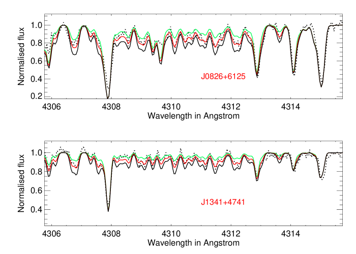
Figure 8.— High-resolution HESP spectra in the CH $G-$band region for SDSS J0826+6125 (upper panel) and SDSS J1341+4741 (lower panel). The red solid line indicates the synthetic spectrum corresponding to the best fit, overplotted with two synthetic spectra with carbon 0.20 dex higher and lower than the adopted value.

5.2. The $\alpha$-Elements

Several magnesium lines were detected in the spectra of our target stars. Two of the lines in the Mg triplet at 5172 Å, and three other lines at 4167 Å, 4702 Å, and 5528 Å, were used to obtain the abundances. The derived [Mg/Fe] ratios for SDSS J0826+6125 and SDSS J1341+4741 are [Mg/Fe] = +0.56 and [Mg/Fe] = +0.71, respectively, values often found among halo stars. The silicon lines at 5268 Å and 6237 Å were too weak to be used for abundance estimates of SDSS J0826+6125, but for SDSS J1341+4741, we obtain [Si/Fe] = +1.0. It should be noted that Si may appear over-abundant for metal-poor stars because LTE results are known to overestimate the true value (Shi et al., 2012).

Eight and eleven Ca I lines were detected in the spectra of SDSS J0826+6125 and SDSS J1341+4741, respectively, including the prominent lines at 4226.73 Å, 4302.53 Å, and 4454.78 Å, and used to measured its abundance. The measurements indicate slightly enhanced ratios of [Ca/Fe] = +0.46 (for SDSS J0826+6125) and [Ca/Fe] = +0.48 (for SDSS J1341+4741). The overall abundance of the $\alpha$-elements is consistent with the typical halo enhancement of [$\alpha$/Fe] = +0.4.

5.3. The Odd-Z Elements

The sodium abundance is determined from the Na $D_{1}$ and $D_{2}$ resonance lines at 5890 Å and 5896 Å. The aluminium abundance is obtained from one of the resonance lines at 3961.5 Å. This line is not the ideal indicator, as it can have large departures from LTE, as discussed by Baumueller & Gehren (1997), who found it to be as large as +0.6 dex. Gratton et al. (2001) showed that incorporation of these corrections improves the agreement between the values of aluminum abundances obtained from this line and the high-excitation infrared doublet at 8773 Å, in the case of globular cluster dwarfs. Hence, we have applied this non-LTE correction to Al in our abundance table. Aluminum is slightly enhanced for SDSS J0826+6125, while Na tracks the iron content of the stars. The scandium content is also very similar to iron. Na and Al are produced by the Ne-Na and Mg-Al cycles in intermediate and massive stars during H-shell burning. Sodium and aluminum in the two stars could be due to a well-mixed ISM, and unlikely to have received direct contribution from intermediate-mass or massive-star winds.

5.4. The Iron-Peak Elements

Iron abundances for SDSS J0826+6125 were calculated using 82 Fe I lines and 7 Fe II lines found in the spectra; a difference of 0.3 dex was noted between the derived abundances. This difference between Fe I and Fe II is in agreement with the NLTE effects explored by Asplund (2005). Iron abundances for SDSS J1341+4741 were calculated using 49 Fe I lines and 7 Fe II lines found in the spectra; a difference of  0.5 dex between the abundance values obtained from these lines was found, which is rather large.

We also detected the iron-peak elements Mn, Cr, Co, Ni, and Zn in our target stars. Mn and Cr are products of incomplete explosive silicon burning, and their abundances decrease with decreasing metallicity (McWilliam et al., 1995; Ryan et al., 1996; Carretta et al., 2002). For SDSS J0826+6125, the abundance of Mn was derived from the resonance Mn triplet at 4030 Å and three weaker lines near 4780 Å. Cr lines are measured from 4 lines, including the stronger ones at 4646  Å and 5206 Å. Products of complete silicon burning, such as Co, Ni, and Zn, have also been found in this star; all of these elements are found to track the iron content. For SDSS J1341+4741, the abundance of Mn was derived from the resonance Mn triplet at 4030 Å and an additional line at 3823 Å. The observed abundances of Mn and Cr are similar to other EMP stars. The abundance derived for Ni using the 4 lines of this element present in the spectrum of SDSS J1341+4741 is clearly higher relative to iron, [Ni/Fe] = +0.35.

5.5. The Neutron-Capture Elements

Strontium and barium are the two neutron-capture elements detected in the spectra of SDSS J1341+4741. Resonance lines of Sr II at 4077 Å and 4215  Å are detected in both of our target stars. SDSS J0826+6125 is found to be under-abundant in both strontium and barium, with abundances of [Sr/Fe] $=-0.63$ and [Ba/Fe] $=-0.95$, respectively. The other neutron-capture elements found in this star are Y and Zr, which are under-abundant as well. SDSS J1341+4741 is also found to be under-abundant in strontium compared to the solar ratio, [Sr/Fe] $=-0.51$. Ba II resonance lines at 4554  Å and 4937 Å were also measured, and exhibited a considerable barium depletion, [Ba/Fe] $=-0.73$. Based on the clear under-abundance of the neutron-capture elements, along with its strong carbon over-abundace, this star can be confidently classified as a CEMP-no star.

Best-fit spectra of the Sr and Ba syntheses for our two stars are shown in Figures 9 and 10.

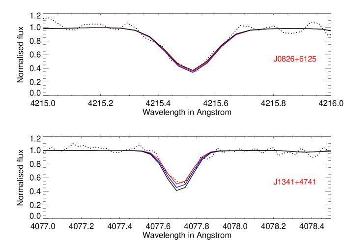
Figure 9.— Synthesis in the Sr II region for SDSS J0826+6125 (upper panel) and SDSS J1341+4741 (lower panel). The red line indicates the best-fit, overplotted with two synthetic spectra with Sr abundance 0.20 dex higher and lower than the adopted value.

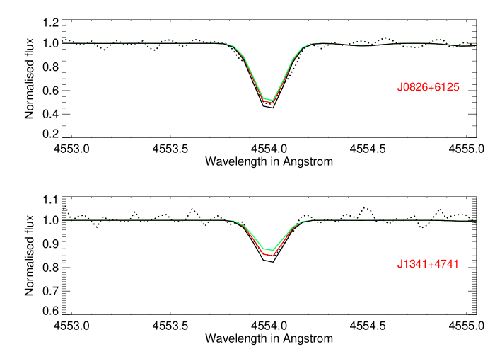
Figure 10.— Synthesis in the Ba II region for SDSS J0826+6125 (upper panel) and SDSS J1341+4741 (lower panel). The red line indicates the best-fit, overplotted with two synthetic spectra with Ba abundance 0.20 dex higher and lower than the adopted value.

5.6. Lithium

Although lithium was not detected in SDSS J0826+6125, there is a strong feature observed in SDSS J1341+4741 at 6707 Å, the Li doublet, from which we obtain an abundance $A$(Li) = 1.95, which is similar to some other CEMP-no stars (e.g , Sivarani et al. 2006, Matsuno et al. 2017). The detection of lithium indicates that this star is unlikely to have experienced AGB binary mass transfer or direct winds from a massive star. Mass transfer from a low-mass AGB would produce large amounts of carbon and deplete lithium, along with the production of $s$-process enhanced material. A $(4-7M_{\odot})$ AGB star that had experienced hot bottom burning produces large nitrogen and very low carbon. There are some models in which AGB stars could produce lithium through the Cameron-Fowler mechanism (Cameron & Fowler, 1971). It is unclear if an AGB with mass 3-4$M_{\odot}$ could explain the observed C, N, low $s$-process elements, and lithium. Evolutionary mixing inside the star in its subgiant phase might deplete the original lithium abundance of the star-forming cloud. The synthesis for this element is shown in Figure 11.

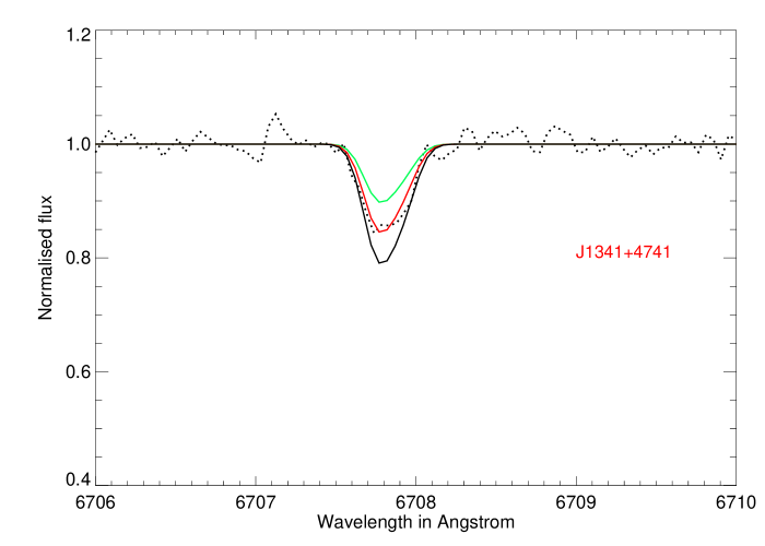
Figure 11.— Synthesis of lithium for SDSS J1341+4741 at 6707 Å. The red line indicates the best-fit, overplotted with two synthetic spectra with Li abundance 0.20 dex higher and lower than the adopted value of A(Li) = 1.95.

6. DISCUSSION

6.1. SDSS J082625.70+612515.10

6.1.1 Carbon, Nitrogen, and the Non-detection of Lithium

In the First Stars VI paper, Spite et al. (2005) found that carbon and nitrogen were anti-correlated, and the faint halo stars could be classified into two groups – “unmixed” stars, which exhibited C enhancement with N depletion, having $A$(Li) between 0.2 and 1.2, and “mixed” stars, which showed [C/Fe] $<0.0$, [N/Fe] $>+0.5$, and Li below the detection threshold. SDSS J0826+6125 clearly falls into the second group. Lithium is a very fragile element, which is destroyed at temperatures in excess of 2.5 million K. Evidence for this can be seen in previous samples of metal-poor stars; the $A$(Li) = 2.3 observed for metal-poor dwarfs starts decreasing as the star ascends the giant branch, to $A$(Li) $<1.2$ for giants (First Stars VII; Bonifacio et al. 2007). The non-detection of lithium for this star could be understood in this way.

In First Stars IX, Spite et al. (2006) argued that such destruction could be taken as a signature of mixing, and placed this mixed group of stars higher up in the giant-branch stage of evolution. Other scenarios for depletion of lithium, such as binary mass transfer, can be eliminated for SDSS J0826+6125, as no such peculiar chemical imprints have been found. During mixing, material from deeper layers where carbon is converted to nitrogen is brought to the stellar surface. Figure 4 of Cayrel et al. (2004) shows the decline in the value of [C/Fe] for temperatures below 4800 K in metal-poor stars, which is again attributed to deep mixing at lower temperatures. With a $T_{\rm eff}$ of 4300 K and a low $\log(g)=0.4$, SDSS J0826+6125 can be placed in the mixed group of stars close to the tip of the red giant branch (RGB). Figure 12 shows the position of the star in the $\log(g)$-$T_{\rm eff}$ plane, compared with other metal-poor halo stars compiled in the SAGA database (Suda et al., 2008). It sits right at the tip of the RGB. Figure 13 compares the [C/N] ratio with metallicity of the halo stars having carbon deficiency (and for which both estimates of carbon and nitrogen are available). The abundance ratio of [C/N] for SDSS J0826+6125  is remakably low compared to other stars at the tip of the RGB.

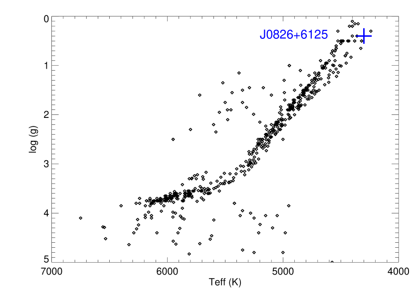
Figure 12.— The position of SDSS J0826+6125 among other EMP halo stars in the log(g)-$T_{\rm eff}$ plane. The position of the star at the tip of the RGB is marked by the blue cross.

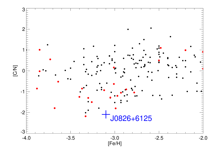
Figure 13.— The very low [C/N] abundance ratio other low-metallicity C-poor halo stars. SDSS J0826+6125 is marked by the blue cross. The red dots mark the stars at the tip of the RGB with log(g)$<$ 1.

6.1.2 The Light Elements

SDSS J0826+6125 exhibits a low Na, high Mg, and low Al content, consistent with the odd-even pattern expected to occur during massive-star nucleosynthesis at low metallicities. A slight enhancement of Na is observed, which could be an imprint of the previous generations of stars which underwent the Ne-Na cycle, as it is not possible to produce these elements in the RGB phase. Such an anomaly could be similar to that seen in globular cluster stars (Gratton et al., 2001, 2004), which have undergone the AGB phase and passed on processed material to a subsequent generation of star formation in a closed system. Unfortunately, other signatures seen in globular cluster stars, such as the C-N-O and O-Na-Mg-Al correlations and anti-correlations (Shetrone, 1996; Gratton et al., 2004; Carretta et al., 2010; Coelho et al., 2011; Mészáros et al., 2015) were not observed in this star.

6.1.3 The Iron-Peak Elements

Abundances of Fe-peak elements (Cr, Mn, Co, and Ni) for metal-poor stars from the SAGA database are plotted, as a function of metallicity, in Figure 14, along with the position of SDSS J0826+6125. This star appears is relatively rich in Co, but poor in Cr, Mn, and Ni, consistent with McWilliam et al. (1995) and Audouze & Silk (1995), who showed the same trends for several stars with metallicity below [Fe/H] $=-2.4$. The relative abundances of the Fe-peak nuclei could be well-explained by their dependence on the mass cut of the progenitor supernova with temperature, which gives rise to a photo-disintegration process (Woosley & Weaver, 1986).

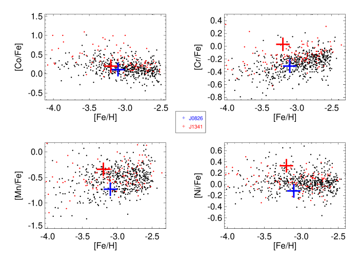
Figure 14.— Distribution of Fe-peak elements for Galactic halo stars. The red dots represent the CEMP-no stars, while black dots represent C-normal halo stars. The two program stars SDSS J0826+6125 and SDSS J1341+4741 are indicated by blue and red crosses, respectively.

6.1.4 The Neutron-Capture Elements

Abundances of both the heavy and light $s$-process elements found in SDSS J0826+6125 are low, which is again consistent with the lack of available neutron flux (Audouze & Silk, 1995). The abundance values are very similar to other EMP giants.

6.1.5 The Asymmetric H$\alpha$ Profile of SDSS J0826+6125 

SDSS J0826+6125  was observed several times, and an asymmetry in the H$\alpha$ profile was noted for all of the spectra. The profile also could not be well-fit with synthetic spectra. The H$\alpha$ profile and its fit with the model spectrum is shown in Figure 15. This could be due to the inadequacy of the 1D stellar models, or it may be due to an extended atmosphere present in the star. The H$\alpha$ profile was also found to be not varying over several observation epochs indicating no ongoing mass transfer. The extended atmosphere could be the result of past mass transfer from an intermediate-mass AGB companion, or mixing due to first dredge up of the star in the RGB phase. It is also possible that the star itself is an AGB star (e.g., Masseron et al. 2006).

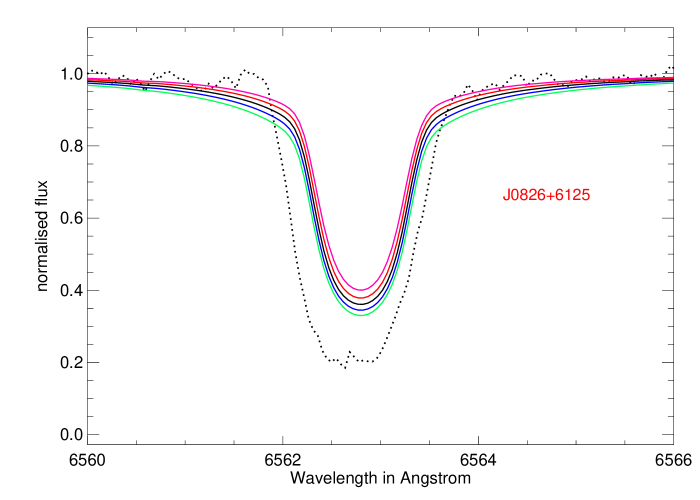
Figure 15.— The strange H$\alpha$ profile of SDSS J0826+6125, for different values of temperature from 4200 K to 4600 K, in steps of 100 K.

6.2. SDSS J134144.60+474128.90

6.2.1 Lithium

We have obtained a measurement of $A$(Li) = 1.95 for SDSS J1341+4741, which is lower than the Spite Plateau (Spite & Spite, 1982) value of $A$(Li) = 2.2$\pm$ 0.1 (Pinsonneault et al., 1999), and much lower than the predicted amount of Li from Big Bang nucleosynthesis ($A$(Li) = 2.75; Steigman 2005). Our limited RV information for this star indicates clear variation, from which we derive a possible period of 116 days. However, we have no other evidence that a mass-transfer event may have occurred. The distribution of lithium for CEMP-no stars, along with other EMP stars, is shown in Figure 16. According to the analysis of Meynet et al. (2010) and Masseron et al. (2012), this star falls close to the edge of Li-depleted stars ($A$(Li) = 2.00 is adopted as the separation between Li-normal and Li-depleted metal-poor stars). A slight depletion from the Spite Plateau value could be attributed to internal mixing of the star, or the observed value of lithium for SDSS J1341+4741 may be the result of several concurrent phenomena.

• The ejected material from the progenitor SN will have depleted lithium abundance along with other nucleosynthetic elements and enhanced carbon (for the case of SDSS J1341+4741) that is mixed with the primordial cloud. Depending upon the dilution factor in the natal cloud, it may be possible to achieve the necessary lithium value (Piau et al., 2006; Meynet et al., 2010; Maeder et al., 2015).

• A Spite Plateau value of Li was present in the natal cloud of SDSS J1341+4741, and it is depleted by thermohaline mixing or meridional circulation (Masseron et al., 2012) in the star. If we consider the current evolutionary state of the star to be in the RGB phase, this could be a viable mechanism.

• Enhanced rotationally-induced mixing in the RGB phase (following Denissenkov & Herwig 2004) can lead to formation of lithium in the star, following depletion of all the primordial lithium. It is very difficult to differentiate between an AGB or a massive rotating star as the precursor using Li as the sole yardstick, as both result in almost the same nucleosynthetic yield of Li (Meynet et al., 2006; Masseron et al., 2012).

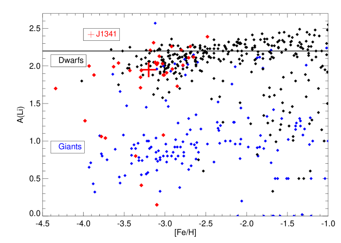
Figure 16.— Comparison of the observed lithium for CEMP-no stars, taken from the SAGA Database. The blue dots mark the EMP giants while black dots are the EMP dwarfs. Red points are the CEMP-no stars. The red cross marks the location of SDSS J1341+4741.

6.2.2 Carbon

According to Spite et al. (2013) and Bonifacio et al. (2015), CEMP stars are distributed along two bands in the $A$(C) vs. [Fe/H] plane. The upper band is centered around $A$(C)$\sim 8.25$, and comprises relatively more metal-rich CEMP-$s$ stars, while the lower band centered around $A$(C) $\sim 6.50$ comprises more metal-poor, and primarily CEMP-no, stars. Further investigation by Hansen et al. (2016a) also led the result that the majority of the stars that are known binaries lie close to the upper band.

By expanding the list of CEMP stars with available high-resolution spectroscopic analyses to include more evolved sub-giants and giants (with the later giants having C abundances corrected for evolutionary mixing effects; Placco et al. 2014), Yoon et al. (2016) demonstrated that the morphology of this abundance space is more complex, with three prominent groups identified in the so-called Yoon-Beers diagram (their Figure 1). They argued that a separation between CEMP-$s$ stars and CEMP-no stars in their sample could be reasonably achieved by splitting the sample at $A$(C) = 7.1, with the Group I CEMP-$s$ stars lying above this level and the Group II and III CEMP-no stars lying below this level. In this classification scheme, SDSS J1341+4741, with $A$(C) $\sim$6.22, can be comfortably identified as a Group II CEMP-no star. Hence, the enhancement of carbon in this star is most likely to be intrinsic to the star (i.e., the C was present in its natal gas), and not the result of mass transfer from an extinct AGB companion. Thus, the elemental-abundance pattern observed from this star is associated with nucloesynthesis from a core collapse SN at early times, perhaps with additional contributions from stars that formed and evolved within its natal gas cloud.

6.2.3 The Light Elements

SDSS J1341+4741 exhibits the low [Na/Fe], high [Mg/Fe], and low [Al/Fe] ratios expected from the odd-even pattern in massive-star nucleosynthesis yields at low metallicities (e.g., Arnett 1971; Truran & Arnett 1971; Peterson 1976; Umeda et al. 2000; Heger & Woosley 2002). The light elements closely follow the overall halo population observed in the Galaxy as well (Cayrel et al., 2004). Following Yoon et al. (2016), SDSS J1341+4741is clearly a member of the Group II stars, and supports a possible mixing and fallback SN as a likely progenitor.

6.2.4 The Iron-Peak Elements

Abundances of Fe-peak elements for SDSS J1341+4741 (Cr, Mn, Co, and Ni) are shown in Figure 14, as a function of [Fe/H], compared with other CEMP-no and C-normal EMP stars compiled from the SAGA database (Suda et al., 2008). One feature that clearly stands out is the over-abundance of Cr and Ni, and to some extent Mn. In the low-metallicity regime, the stars are expected to show signatures of Type II SNe nucleosynthesis. All three elements play key roles in determining the progenitor population in the halo and the subsequent SNe yields. A decrease in [Cr$/$Fe] and [Mn/Fe] with decreasing [Fe/H] should be accompanied with enhancement in [Co/Fe], as a result of deeper mass cuts in the progenitor SNe (refer to Figure 9 of Nakamura et al. 1999). However, enhancement in both [Cr/Fe] and [Mn/Fe] can be explained by an excess of neutrons as well. Since neutron excess is a function of metallicity, we have plotted [Cr/Fe] vs. [Mn/Fe] in Figure 17 to eliminate the trend with Fe abundance (following, e.g., Carretta et al. 2002). In this plot, our program star occupies a relatively higher position amidst the population of CEMP-no stars. From Heger & Woosley (2002), Heger & Woosley (2010), and Qian & Wasserburg (2002), it is known that very massive stars ($80<M/M_{\odot}<240)$ belonging to Population III explode as pair-instability SNe, which should not produce a correlation between [Cr/Fe] and [Mn/Fe]. Thus, the presence of this correlation points us towards Type II SNe associated with a relatively high-mass ($M/M_{\odot}<80$), but not extremely high-mass, progenitor.

Nickel is an extremely important element to gain further insight into the nature of the progenitor of SDSS J1341+4741. The depth of the gravitational potential and amount of neutrino-absorbing material in the models are the two factors that compete for the production of Ni in Type II SNe. In very massive ($M/M_{\odot}>30$) stars the deeper gravitational potential restricts nickel from being ejected due to fallback, while intermediate-mass ($10<M/M_{\odot}<20$) stars eject large amounts of Ni because of a large neutrino-absorbing region (Nakamura et al., 1999). Thus, enhancement of Ni also points in the same direction, that the progenitor is likely to be a massive ($20<M/M_{\odot}<30$) star exploding as a Type II SNe in the early Galaxy. The observations support the hypothesis of a mixing and fallback model (Nomoto et al., 2013) with a lower degree of fallback, so as to eject a larger mass of ⁵⁶Ni.

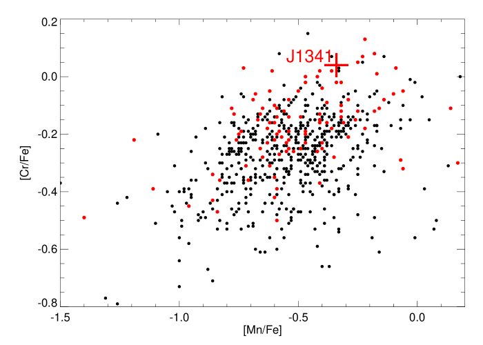
Figure 17.— The relative enhancement of Cr and Mn for SDSS J1341+4741, shown as a red cross, in the [Cr/Fe] vs. [Mn/Fe] space. Red dots mark the CEMP-no stars while the black dots mark the EMP stars.

6.2.5 The Neutron-Capture Elements

The first $s$-process peak element Sr and the second $s$-process peak element Ba have been detected in both SDSS J0826+6125 and SDSS J1341+4741, and they exhibit under-abundances. The ratio of light to heavier neutron-capture elements are sensitive to the nature of the progenitors. Neutron star mergers are expected to produce heavy neutron-capture elements (e.g., Argast et al. 2004) – and have been observed to do so in the kilonova SSS17a associated with GW170817 (Kilpatrick et al., 2017), which exhibited clear evidence for the presence of unstable isotopes created by the $r$-process (Drout et al., 2017; Shappee et al., 2017). SNe with jets (e.g., Winteler et al. 2012; Nishimura et al. 2015) may also produce heavy neutron-capture elements. Formation of these systems may depend on the environment as well.

6.2.6 Nature of the Binary Companions of SDSS J0826+6125 and SDSS J1341+4741

Both of the program stars exhibit clear RV variations, indicating the likely presence of a binary companion. In the case of SDSS J0826+6125, the enhanced abundances of N and under-abundance of C indicates possible mixing of the atmosphere with CN-cycle products. This can result from first dredge-up mixing in the star, which is currently in the RGB, following mass transfer from an intermediate-mass AGB star that might have gone through hot bottom burning (Lau et al., 2007; Suda et al., 2012). The low $\log(g)$ value of the star supports RGB mixing, although AGB mass transfer cannot be ruled out. The non-detection of Li and peculiar H$\alpha$ profiles could indicate either internal mixing or binary mass transfer as well. In the case of an intermediate-mass AGB that goes through hot bottom burning, the temperatures are sufficiently high for the star to operate the CNO cycle. In that case, SDSS J0826+6125 may be a true nitrogen-enhanced metal-poor (NEMP; see Johnson et al. 2007; Pols et al. 2009; Pols et al. 2012) star, which are known to exist, but are relatively rare.

In the case of SDSS J1341+4741, the binary companion did not likely contribute through a mass-transfer event, since the Li abundance in the star is similar to other EMP stars, although it is lower than the Spite Plateau value. The mild depletion of Li could be due to binary-induced mixing or internal mixing of the star during its sub-giant phase. It may well be worthwhile to mount a RV-monitoring campaign for this and other Li-depleted EMP stars to test for a possible binary-star origin to the declining lithium abundance problem for stars with [Fe/H] $<-3.0$.

6.3. CEMP-no and EMP Stars

From the above discussion, and based on previous studies, it is evident that CEMP-no and C-normal EMP stars have very different origins. Even within the sub-class of CEMP-no stars, there may well be different types of progenitors. As discussed by Yoon et al. (2016), the Group II CEMP-no stars could be associated with the faint mixing and fallback SNe, whereas the Group III CEMP-no stars can be attributed to the spinstar models, with a number of exceptions for both the classes (Meynet et al., 2006; Nomoto et al., 2013). See also the discussion of the progenitors for CEMP-no stars by Placco et al. (2016). Some of the CEMP-no stars lying in the low $A$(C) region may have a binary component, but no mass transfer is supposed to have taken place (Starkenburg et al., 2014; Bonifacio et al., 2015; Yoon et al., 2016), which is further strengthened by the only “slight” depletion of Li in SDSS J1341+4741, as described in the previous section. Iron-peak elements can provide valuable insights regarding the nucleosynthetic yields of their progenitor supernovae, as these elements cannot be produced or modified during the post main-sequence evolutionary stages of the star. Figure 14 shows the distribution of some key Fe-peak elements for both CEMP-no and C-normal EMP stars. Visual inspection suggests that Cr and Co are enhanced for the CEMP-no population. We have compiled data from SAGA databse to see if there is an enhancement of Cr in CEMP-no stars. The fit is given in Figure 18 for [Cr/Fe]. There is a slight offset between the EMP and CEMP-no stars, but they exhibit similar increasing trends of [Cr/Fe] with [Fe/H]. We have checked, and these behaviors apply to both dwarfs and giants. Similar offset could also be noted for Co. Lai et al. (2008) and Bonifacio et al. (2009) have considered the discrepancies in the behavior of Cr between giants and dwarfs, since Cr II could be measured only in giants, while Cr I is a resonance line, and could suffer substantial NLTE effects. However, such issues are not expected to play a substantial role when we compare only giants with giants or dwarfs with dwarfs. Temperature and gravity do not play a major role in deviations from LTE abundances (Bergemann & Cescutti, 2010), so we have not used them to further refine our sample from the archival data. Enhancement in [Cr/Fe] for CEMP-no stars with respect to C-normal EMP stars can play a key role for understanding of the SNe ejecta and relevant mass cuts. It would be very interesting to investigate the origin for this discrepancy.

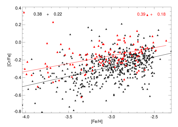
Figure 18.— Linear fit for CEMP-no and C-normal EMP stars. Red is used for CEMP-no stars while black is used for EMP stars. The slope and $\sigma$ are shown for each fit in the corresponding color.

7. Conclusion

We have derived LTE abundances for SDSS J082625.70+612515.10; it is mostly consistent with behavior of other halo stars. The depletion in carbon and enhancement in nitrogen could be due to internal mixing within the star. It is unlikely that self enrichment similar to that is seen in globular clusters has occured, due to the overabundance in oxygen. The peculiar H$\alpha$ profiles of SDSS J0826+6125 also supports the possibility of mixing that might occur in an extended atmosphere. The radial-velocity variation strongly suggests this star is a member of a binary system, but it is likely there is no ongoing mass transfer, due to non-variable peculiar H$\alpha$ profile over a period of year.

SDSS J134144.60+474128.90 is a CEMP-no type star, and likely to be a member of binary system. The lithium is detected and midly depleted, similar to other EMP stars. Lithium in EMP dwarfs and CEMP-no stars exhibit similar trends at different metallicities. Below [Fe/H] $<-3.0$, EMP and CEMP-no stars often have lithium abundance below the Spite Plateau. We also studied the trends of heavy elements among EMP and CEMP stars. At a given metallicity, CEMP-no stars appear to have larger abundances of Cr. This might provide important clues to the nature of the progenitors that contributed to the origin of carbon.

8. Acknowledgement

We would like to take this opportunity to thank the HESP team for succesful installation and maintenance of the high-resolution spectroscope at the Hanle telescope, despite the numerous challenges and hurdles that were encountered along the way. We would specially like to thank Amit Kumar, M N Anand, Sriram and Kathiravan for their efforts. We also extend our gratitude towards the observation team, namely Kiran B.S, Pramod Kumar,Lakshmi Prasad and Venkatesh Shankar for their tireless effort.

T.C.B. acknowledges partial support from grant PHY 14-30152 (Physics Frontier Center/JINA-CEE), awarded by the U.S. National Science Foundation (NSF). T.M. acknowledges support provided by the Spanish Ministry of Economy and Competitiveness (MINECO) under grants AYA−2014−58082-P and AYA-2017-88254-P.

Table 7Linelist for SDSS J0826+6125

Species	$\lambda$	obs.eqw	error	Abundance
CaI	4425.437	34.000	1.806	3.284
CaI	4435.679	27.600	1.628	3.239
CaI	5594.462	30.300	1.705	3.574
CaI	6122.217	61.900	2.437	3.729
CaI	6162.173	82.000	2.805	3.867
CaI	6439.075	53.600	2.268	3.598
CaI	6449.808	8.000	0.876	3.870
TiI	4981.731	54.800	2.293	1.884
TiI	4991.065	52.700	2.249	1.970
TiI	4999.503	40.600	1.974	1.851
TiI	5007.210	52.100	2.236	2.188
TiI	5014.187	49.600	2.182	2.301
TiI	5064.653	30.200	1.702	1.804
TiI	5210.385	43.000	2.031	1.905
TiII	4470.857	45.400	2.087	2.107
TiII	5129.152	39.400	1.945	2.068
TiII	5154.070	44.900	2.076	2.275
TiII	5185.913	28.000	1.639	1.913
TiII	5188.680	72.500	2.638	2.054
TiII	5381.015	36.100	1.861	2.234
CrI	4545.945	7.700	0.860	1.986
CrI	4646.148	44.400	2.064	2.445
CrI	5206.038	81.300	2.793	2.170
CrI	5298.277	10.600	1.009	1.915
CrI	5348.312	6.700	0.802	1.849
CrII	4558.650	8.500	0.903	2.249
CrII	4588.199	11.400	1.046	2.574

Species	$\lambda$	obs.eqw	error	Abundance
FeI	4147.669	68.747	2.569	4.283
FeI	4174.913	72.100	2.631	4.513
FeI	4175.636	23.000	1.486	3.837
FeI	4202.029	125.300	3.468	4.195
FeI	4206.697	90.700	2.950	4.492
FeI	4216.220	119.900	3.392	10.028
FeI	4233.603	63.000	2.459	3.989
FeI	4250.787	143.600	3.712	4.707
FeI	4260.474	89.000	2.923	3.780
FeI	4415.123	124.700	3.460	4.140
FeI	4442.339	73.700	2.660	4.481
FeI	4447.717	83.500	2.831	4.900
FeI	4489.739	99.300	3.087	4.696
FeI	4528.614	97.500	3.059	4.521
FeI	4602.941	69.399	2.581	4.353
FeI	4733.592	32.500	1.766	4.349
FeI	4736.773	27.200	1.616	4.294
FeI	4871.318	64.599	2.490	4.216
FeI	4872.138	68.300	2.560	4.464
FeI	4890.755	80.000	2.771	4.539
FeI	4891.492	85.983	2.873	4.212
FeI	4903.310	47.600	2.137	4.394

Species	$\lambda$	obs.eqw	error	Abundance
FeI	4918.994	82.600	2.816	4.543
FeI	4920.502	99.200	3.086	4.563
FeI	4939.687	68.560	2.565	4.425
FeI	4994.130	95.200	3.023	4.709
FeI	5001.864	34.500	1.820	4.478
FeI	5014.943	18.900	1.347	4.499
FeI	5049.820	73.900	2.663	4.559
FeI	5051.635	106.799	3.202	4.689
FeI	5068.766	33.000	1.780	4.277
FeI	5079.740	69.700	2.586	4.504
FeI	5083.339	89.400	2.929	4.586
FeI	5123.720	64.100	2.480	4.332
FeI	5127.359	69.361	2.580	4.447
FeI	5142.928	79.200	2.757	4.544
FeI	5150.840	74.400	2.672	4.350
FeI	5166.282	89.600	2.932	4.306
FeI	5171.596	99.900	3.096	4.107
FeI	5192.344	78.394	2.743	4.607
FeI	5194.942	104.700	3.170	4.806
FeI	5216.274	85.100	2.858	4.588
FeI	5225.526	47.600	2.137	4.425
FeI	5232.940	92.300	2.976	4.439
FeI	5247.050	36.700	1.877	4.372
FeI	5250.209	49.400	2.177	4.593
FeI	5250.646	39.300	1.942	4.562
FeI	5266.555	61.700	2.433	4.287
FeI	5270.356	148.900	3.780	4.794
FeI	5283.621	49.100	2.171	4.375

Species	$\lambda$	obs.eqw	error	Abundance
FeI	5307.361	34.300	1.814	4.479
FeI	5324.179	69.500	2.583	4.403
FeI	5332.900	41.600	1.998	4.385
FeI	5339.929	28.000	1.639	4.194
FeI	5393.168	34.900	1.830	4.432
FeI	5397.128	140.200	3.668	4.309
FeI	5405.775	147.000	3.756	4.414
FeI	5415.199	29.888	1.694	4.348
FeI	5434.524	132.100	3.561	4.446
FeI	5497.516	89.501	2.931	4.384
FeI	5501.465	83.700	2.834	4.436
FeI	5506.779	83.400	2.829	4.252
FeI	5576.089	21.800	1.446	4.572
FeI	5572.842	44.000	2.055	4.274
FeI	5624.542	21.894	1.450	4.304
FeI	6065.482	39.500	1.947	4.410
FeI	6136.615	56.671	2.332	4.304
FeI	6137.692	50.000	2.191	4.383
FeI	6230.723	69.821	2.589	4.537
FeI	6252.555	58.000	2.359	4.572
FeI	6265.134	25.900	1.577	4.527
FeI	6335.331	28.700	1.660	4.317
FeI	6358.698	31.300	1.733	4.763
FeI	6393.601	53.451	2.265	4.230
FeI	6421.351	36.200	1.864	4.442
FeI	6430.846	62.100	2.441	4.605

Species	$\lambda$	obs.eqw	error	Abundance
FeI	6494.980	78.500	2.745	4.429
FeI	6592.914	40.400	1.969	4.434
FeII	4233.172	94.400	3.010	5.001
FeII	4491.405	17.600	1.300	4.136
FeII	4583.837	68.400	2.562	4.458
FeII	4923.921	106.100	3.191	4.993
FeII	5018.440	103.600	3.153	4.776
FeII	5197.568	33.800	1.801	13.002
FeII	5316.615	77.600	2.729	4.910
NiI	4855.406	8.100	0.882	3.040
NiI	6643.629	11.300	1.041	2.946
NiI	6767.768	16.200	1.247	3.165
ZnI	4722.153	11.500	1.051	1.668
ZnI	4810.528	9.300	0.945	1.434

The errors are computed using Cayrel’s relation (Cayrel de Strobel & Spite, 1988).

Table 8Linelist for SDSS J1341+4741

Species	$\lambda$	obs.eqw	error	Abundance
SiI	5268.387	4.600	0.664	5.457
SiI	6237.319	4.200	0.635	5.358
CaI	4226.728	112.700	3.289	3.221
CaI	4283.011	10.300	0.994	3.401
CaI	4302.528	23.800	1.511	3.368
CaI	4318.652	18.700	1.340	3.710
CaI	4425.437	27.400	1.622	3.910
CaI	4454.779	39.600	1.950	3.558
CaI	4585.865	12.200	1.082	3.679
CaI	5857.451	9.100	0.935	3.834
CaI	6122.217	28.700	1.660	3.959
CaI	6162.173	32.700	1.772	3.841
CaI	6439.075	21.600	1.440	3.677
TiI	4533.241	15.600	1.224	2.419
TiI	4981.731	13.100	1.121	2.288
TiI	4991.065	6.000	0.759	2.036
TiI	4999.503	9.800	0.970	2.368
TiII	4012.385	17.500	1.296	1.789
TiII	4028.343	21.100	1.423	2.522
TiII	4163.648	3.200	0.554	1.598
TiII	4171.910	3.500	0.580	1.739
TiII	4290.219	49.800	2.186	2.259
TiII	4300.049	53.300	2.262	1.899
TiII	4312.864	22.400	1.466	1.933
TiII	4395.033	58.600	2.372	1.888
TiII	4443.794	52.200	2.238	1.965

Species	$\lambda$	obs.eqw	error	Abundance
TiII	4468.507	57.900	2.357	2.013
TiII	4501.273	48.400	2.155	1.974
TiII	4533.969	49.800	2.186	1.904
TiII	4563.761	36.600	1.874	1.887
TiII	4571.968	31.800	1.747	1.599
CrI	4254.332	54.600	2.289	2.187
CrI	4274.796	59.800	2.396	2.377
CrI	4289.716	46.200	2.106	2.240
CrI	5204.506	14.600	1.184	2.296
CrI	5206.038	31.900	1.750	2.504
CrI	5208.419	39.100	1.937	2.509
CrI	4824.127	4.300	0.642	2.834
MnI	3823.507	37.100	1.887	3.290
MnI	4030.753	41.100	1.986	1.622
MnI	4033.062	15.200	1.208	1.178
MnI	4034.483	17.900	1.311	1.449
MnI	4823.524	3.800	0.604	2.165
FeI	4005.242	72.350	2.635	4.325
FeI	4045.812	109.200	3.237	4.339
FeI	4132.058	73.770	2.661	4.379
FeI	4143.868	77.740	2.732	4.299
FeI	4187.039	41.910	2.006	4.452
FeI	4187.795	36.600	1.874	4.310
FeI	4198.304	29.080	1.671	4.306
FeI	4202.029	73.499	2.656	4.140
FeI	4227.427	19.970	1.384	3.934
FeI	4250.119	31.760	1.746	4.095

Species	$\lambda$	obs.eqw	error	Abundance
FeI	4250.787	66.470	2.526	4.165
FeI	4260.474	63.579	2.470	4.213
FeI	4271.154	47.860	2.143	4.437
FeI	4271.760	92.450	2.979	3.977
FeI	4325.762	83.979	2.839	3.897
FeI	4375.930	41.550	1.997	4.511
FeI	4383.545	112.400	3.284	4.508
FeI	4404.750	86.770	2.886	4.355
FeI	4415.122	69.280	2.579	4.522
FeI	4427.310	31.930	1.751	4.399
FeI	4528.614	38.710	1.927	4.440
FeI	4531.148	21.030	1.421	4.644
FeI	4583.721	25.720	1.571	7.103
FeI	4871.318	28.190	1.645	4.433
FeI	4872.138	26.150	1.584	4.603
FeI	4891.492	40.500	1.972	4.401
FeI	4918.994	26.150	1.584	4.360
FeI	5006.119	16.280	1.250	4.348
FeI	5041.756	13.310	1.130	4.420
FeI	5171.596	26.600	1.598	4.370
FeI	5194.942	20.500	1.403	4.603
FeI	5216.274	11.600	1.055	4.429
FeI	5232.940	38.020	1.910	4.387
FeI	5266.555	19.990	1.385	4.388
FeI	5269.537	76.789	2.715	4.240
FeI	5324.179	27.990	1.639	4.632
FeI	5328.039	79.800	2.767	4.483
FeI	5328.532	22.770	1.478	4.404

Species	$\lambda$	obs.eqw	error	Abundance
FeI	5371.490	67.410	2.544	4.445
FeI	5397.128	55.110	2.300	4.490
FeI	5405.775	58.820	2.376	4.487
FeI	5429.697	57.280	2.345	4.474
FeI	5434.524	36.540	1.873	4.386
FeI	5446.917	56.490	2.328	4.522
FeI	5455.609	45.910	2.099	4.532
FeI	5572.842	12.470	1.094	4.478
FeI	5615.644	24.400	1.530	4.603
FeI	6230.723	16.000	1.239	4.670
FeI	6494.980	18.970	1.349	4.552
FeII	4233.172	30.390	1.708	4.243
FeII	4508.288	15.630	1.225	4.494
FeII	4515.339	5.290	0.713	4.132
FeII	4522.634	7.240	0.834	3.890
FeII	4555.893	2.260	0.466	3.527
FeII	4583.837	25.720	1.571	4.294
FeII	4923.927	48.280	2.153	4.255
CoI	4092.384	7.900	0.871	2.267
CoI	4121.311	11.400	1.046	1.823
NiI	3807.138	30.300	1.705	2.603
NiI	4401.538	7.000	0.820	3.374
NiI	4459.027	22.000	1.453	4.258
NiI	5476.900	20.600	1.406	3.348

The errors are computed using Cayrel’s relation (Cayrel de Strobel & Spite, 1988) .

References

- Alonso et al. (1996) Alonso, A., Arribas, S., & Martinez-Roger, C. 1996, A&A, 313, 873
- Alonso et al. (1999) Alonso, A., Arribas, S., & Martínez-Roger, C. 1999, A&AS, 140, 261
- Alvarez & Plez (1998) Alvarez, R., & Plez, B. 1998, A&A, 330, 1109
- Anders et al. (2014) Anders, F., et al. 2014, A&A, 564, A115
- Aoki et al. (2007) Aoki, W., Beers, T. C., Christlieb, N., Norris, J. E., Ryan, S. G., & Tsangarides, S. 2007, ApJ, 655, 492
- Aoki et al. (2013) Aoki, W., et al. 2013, AJ, 145, 13
- Argast et al. (2004) Argast, D., Samland, M., Thielemann, F.-K., & Qian, Y.-Z. 2004, A&A, 416, 997
- Arnett (1971) Arnett, W. D. 1971, ApJ, 166, 153
- Asplund (2005) Asplund, M. 2005, Highlights of Astronomy, 13, 542
- Asplund et al. (2009) Asplund, M., Grevesse, N., Sauval, A. J., & Scott, P. 2009, ARA&A, 47, 481
- Audouze & Silk (1995) Audouze, J., & Silk, J. 1995, ApJ, 451, L49
- Baumueller & Gehren (1997) Baumueller, D., & Gehren, T. 1997, A&A, 325, 1088
- Bayo et al. (2008) Bayo, A., Rodrigo, C., Barrado Y Navascués, D., Solano, E., Gutiérrez, R., Morales-Calderón, M., & Allard, F. 2008, A&A, 492, 277
- Beers & Christlieb (2005) Beers, T. C., & Christlieb, N. 2005, ARA&A, 43, 531
- Beers et al. (1985) Beers, T. C., Preston, G. W., & Shectman, S. A. 1985, AJ, 90, 2089
- Beers et al. (1992) —. 1992, AJ, 103, 1987
- Beers et al. (2017) Beers, T. C., et al. 2017, ApJ, 835, 81
- Bergemann & Cescutti (2010) Bergemann, M., & Cescutti, G. 2010, A&A, 522, A9
- Bonifacio et al. (2007) Bonifacio, P., et al. 2007, A&A, 462, 851
- Bonifacio et al. (2009) —. 2009, A&A, 501, 519
- Bonifacio et al. (2015) —. 2015, A&A, 579, A28
- Bromm et al. (2009) Bromm, V., Yoshida, N., Hernquist, L., & McKee, C. F. 2009, Nature, 459, 49
- Cameron & Fowler (1971) Cameron, A. G. W., & Fowler, W. A. 1971, ApJ, 164, 111
- Carretta et al. (2010) Carretta, E., Bragaglia, A., D’Orazi, V., Lucatello, S., & Gratton, R. G. 2010, A&A, 519, A71
- Carretta et al. (2002) Carretta, E., Gratton, R., Cohen, J. G., Beers, T. C., & Christlieb, N. 2002, AJ, 124, 481
- Castelli & Kurucz (2004) Castelli, F., & Kurucz, R. L. 2004, ArXiv Astrophysics e-prints
- Cayrel et al. (2004) Cayrel, R., et al. 2004, A&A, 416, 1117
- Cayrel de Strobel & Spite (1988) Cayrel de Strobel, G., & Spite, M., eds. 1988, IAU Symposium, Vol. 132, The impact of very high S/N spectroscopy on stellar physics: proceedings of the 132nd Symposium of the International Astronomical Union held in Paris, France, June 29-July 3, 1987.
- Chiaki et al. (2018) Chiaki, G., Susa, H., & Hirano, S. 2018, MNRAS, 475, 4378
- Chiaki et al. (2017) Chiaki, G., Tominaga, N., & Nozawa, T. 2017, MNRAS, 472, L115
- Chiappini (2013) Chiappini, C. 2013, Astronomische Nachrichten, 334, 595
- Choplin et al. (2016) Choplin, A., Maeder, A., Meynet, G., & Chiappini, C. 2016, A&A, 593, A36
- Christlieb (2003) Christlieb, N. 2003, in Reviews in Modern Astronomy, Vol. 16, Reviews in Modern Astronomy, ed. R. E. Schielicke, 191
- Coelho et al. (2011) Coelho, P., Percival, S. M., & Salaris, M. 2011, ApJ, 734, 72
- Cooke & Madau (2014) Cooke, R. J., & Madau, P. 2014, The Astrophysical Journal, 791, 116
- Cowan & Rose (1977) Cowan, J. J., & Rose, W. K. 1977, ApJ, 212, 149
- de Laverny et al. (2012) de Laverny, P., Recio-Blanco, A., Worley, C. C., & Plez, B. 2012, A&A, 544, A126
- Denissenkov & Herwig (2004) Denissenkov, P. A., & Herwig, F. 2004, ApJ, 612, 1081
- Drout et al. (2017) Drout, M. R., et al. 2017, Science, 358, 1570
- Eisenstein et al. (2011) Eisenstein, D. J., et al. 2011, AJ, 142, 72
- Fernández-Alvar et al. (2016) Fernández-Alvar, E., Allende Prieto, C., Beers, T. C., Lee, Y. S., Masseron, T., & Schneider, D. P. 2016, A&A, 593, A28
- Frebel & Norris (2015) Frebel, A., & Norris, J. E. 2015, ARA&A, 53, 631
- Frebel et al. (2006) Frebel, A., et al. 2006, ApJ, 652, 1585
- Fulbright et al. (2010) Fulbright, J. P., et al. 2010, ApJ, 724, L104
- García Pérez et al. (2013) García Pérez, A. E., et al. 2013, ApJ, 767, L9
- Gratton et al. (2004) Gratton, R., Sneden, C., & Carretta, E. 2004, ARA&A, 42, 385
- Gratton et al. (2001) Gratton, R. G., et al. 2001, A&A, 369, 87
- Grevesse et al. (2015) Grevesse, N., Scott, P., Asplund, M., & Sauval, A. J. 2015, A&A, 573, A27
- Gustafsson et al. (2008) Gustafsson, B., Edvardsson, B., Eriksson, K., Jørgensen, U. G., Nordlund, Å., & Plez, B. 2008, A&A, 486, 951
- Hampel et al. (2016) Hampel, M., Stancliffe, R. J., Lugaro, M., & Meyer, B. S. 2016, ApJ, 831, 171
- Hansen et al. (2016a) Hansen, T. T., Andersen, J., Nordström, B., Beers, T. C., Placco, V. M., Yoon, J., & Buchhave, L. A. 2016a, A&A, 586, A160
- Hansen et al. (2016b) —. 2016b, A&A, 588, A3
- Heger & Woosley (2002) Heger, A., & Woosley, S. E. 2002, ApJ, 567, 532
- Heger & Woosley (2010) —. 2010, ApJ, 724, 341
- Ivezić et al. (2012) Ivezić, Ž., Beers, T. C., & Jurić, M. 2012, ARA&A, 50, 251
- Johnson et al. (2007) Johnson, J. A., Herwig, F., Beers, T. C., & Christlieb, N. 2007, ApJ, 658, 1203
- Kilpatrick et al. (2017) Kilpatrick, C. D., et al. 2017, Science, 358, 1583
- Lai et al. (2008) Lai, D. K., Bolte, M., Johnson, J. A., Lucatello, S., Heger, A., & Woosley, S. E. 2008, ApJ, 681, 1524
- Lau et al. (2007) Lau, H. H. B., Stancliffe, R. J., & Tout, C. A. 2007, MNRAS, 378, 563
- Lee et al. (2017) Lee, Y. S., Beers, T. C., Kim, Y. K., Placco, V., Yoon, J., Carollo, D., Masseron, T., & Jung, J. 2017, ApJ, 836, 91
- Lee et al. (2013) Lee, Y. S., et al. 2013, AJ, 146, 132
- Li et al. (2015) Li, H.-N., Zhao, G., Christlieb, N., Wang, L., Wang, W., Zhang, Y., Hou, Y., & Yuan, H. 2015, ApJ, 798, 110
- Lucatello et al. (2005) Lucatello, S., Tsangarides, S., Beers, T. C., Carretta, E., Gratton, R. G., & Ryan, S. G. 2005, The Astrophysical Journal, 625, 825
- Maeder & Meynet (2015) Maeder, A., & Meynet, G. 2015, A&A, 580, A32
- Maeder et al. (2015) Maeder, A., Meynet, G., & Chiappini, C. 2015, A&A, 576, A56
- Masseron et al. (2012) Masseron, T., Johnson, J. A., Lucatello, S., Karakas, A., Plez, B., Beers, T. C., & Christlieb, N. 2012, ApJ, 751, 14
- Masseron et al. (2006) Masseron, T., et al. 2006, A&A, 455, 1059
- Matsuno et al. (2017) Matsuno, T., Aoki, W., Beers, T. C., Lee, Y. S., & Honda, S. 2017, AJ, 154, 52
- McWilliam (1998) McWilliam, A. 1998, AJ, 115, 1640
- McWilliam et al. (1995) McWilliam, A., Preston, G. W., Sneden, C., & Searle, L. 1995, AJ, 109, 2757
- Mészáros et al. (2015) Mészáros, S., et al. 2015, AJ, 149, 153
- Meynet et al. (2006) Meynet, G., Ekström, S., & Maeder, A. 2006, A&A, 447, 623
- Meynet et al. (2010) Meynet, G., Hirschi, R., Ekstrom, S., Maeder, A., Georgy, C., Eggenberger, P., & Chiappini, C. 2010, A&A, 521, A30
- Nakamura et al. (1999) Nakamura, T., Umeda, H., Nomoto, K., Thielemann, F.-K., & Burrows, A. 1999, ApJ, 517, 193
- Nishimura et al. (2015) Nishimura, N., Takiwaki, T., & Thielemann, F.-K. 2015, ApJ, 810, 109
- Nomoto et al. (2013) Nomoto, K., Kobayashi, C., & Tominaga, N. 2013, ARA&A, 51, 457
- Paegert et al. (2015) Paegert, M., et al. 2015, AJ, 149, 186
- Peterson (1976) Peterson, R. C. 1976, ApJ, 206, 800
- Piau et al. (2006) Piau, L., Beers, T. C., Balsara, D. S., Sivarani, T., Truran, J. W., & Ferguson, J. W. 2006, ApJ, 653, 300
- Pinsonneault et al. (1999) Pinsonneault, M. H., Walker, T. P., Steigman, G., & Narayanan, V. K. 1999, ApJ, 527, 180
- Placco et al. (2016) Placco, V. M., et al. 2016, ApJ, 833, 21
- Plez & Cohen (2005) Plez, B., & Cohen, J. G. 2005, A&A, 434, 1117
- Pols et al. (2009) Pols, O. R., Izzard, R. G., Glebbeek, E., & Stancliffe, R. J. 2009, PASA, 26, 327
- Pols et al. (2012) Pols, O. R., Izzard, R. G., Stancliffe, R. J., & Glebbeek, E. 2012, A&A, 547, A76
- Qian & Wasserburg (2002) Qian, Y.-Z., & Wasserburg, G. J. 2002, ApJ, 567, 515
- Ramírez & Meléndez (2005) Ramírez, I., & Meléndez, J. 2005, ApJ, 626, 465
- Ryan et al. (1996) Ryan, S. G., Norris, J. E., & Beers, T. C. 1996, ApJ, 471, 254
- Scott et al. (2015a) Scott, P., Asplund, M., Grevesse, N., Bergemann, M., & Sauval, A. J. 2015a, A&A, 573, A26
- Scott et al. (2015b) Scott, P., et al. 2015b, A&A, 573, A25
- Shappee et al. (2017) Shappee, B. J., et al. 2017, Science, 358, 1574
- Sharma et al. (2018) Sharma, M., Theuns, T., Frenk, C. S., & Cooke, R. J. 2018, MNRAS, 473, 984
- Shetrone (1996) Shetrone, M. D. 1996, in Astronomical Society of the Pacific Conference Series, Vol. 92, Formation of the Galactic Halo…Inside and Out, ed. H. L. Morrison & A. Sarajedini, 383
- Shi et al. (2012) Shi, J. R., Takada-Hidai, M., Takeda, Y., Tan, K. F., Hu, S. M., Zhao, G., & Cao, C. 2012, ApJ, 755, 36
- Sivarani et al. (2006) Sivarani, T., et al. 2006, A&A, 459, 125
- Smith et al. (2015) Smith, B. D., Wise, J. H., O’Shea, B. W., Norman, M. L., & Khochfar, S. 2015, MNRAS, 452, 2822
- Spite & Spite (1982) Spite, F., & Spite, M. 1982, A&A, 115, 357
- Spite et al. (2013) Spite, M., Caffau, E., Bonifacio, P., Spite, F., Ludwig, H.-G., Plez, B., & Christlieb, N. 2013, A&A, 552, A107
- Spite et al. (2005) Spite, M., et al. 2005, A&A, 430, 655
- Spite et al. (2006) —. 2006, A&A, 455, 291
- Starkenburg et al. (2014) Starkenburg, E., Shetrone, M. D., McConnachie, A. W., & Venn, K. A. 2014, MNRAS, 441, 1217
- Steigman (2005) Steigman, G. 2005, Physica Scripta Volume T, 121, 142
- Suda et al. (2008) Suda, T., et al. 2008, PASJ, 60, 1159
- Suda et al. (2012) Suda, T., et al. 2012, AGB evolution and nucleosynthesis at low-metallicity constrained by the star formation history of our galaxy, ed. J. Lattanzio, A. Karakas, & G. Dracoulis (Scuola Internazionale Superiore di Studi Avanzati (S I S S A)), 1 – 5
- Susmitha Rani et al. (2016) Susmitha Rani, A., Sivarani, T., Beers, T. C., Fleming, S., Mahadevan, S., & Ge, J. 2016, MNRAS, 458, 2648
- Tominaga et al. (2014) Tominaga, N., Iwamoto, N., & Nomoto, K. 2014, ApJ, 785, 98
- Truran & Arnett (1971) Truran, J. W., & Arnett, W. D. 1971, Ap&SS, 11, 430
- Umeda & Nomoto (2003) Umeda, H., & Nomoto, K. 2003, Nature, 422, 871
- Umeda & Nomoto (2005) —. 2005, ApJ, 619, 427
- Umeda et al. (2000) Umeda, H., Nomoto, K., & Nakamura, T. 2000, in The First Stars, ed. A. Weiss, T. G. Abel, & V. Hill, 150
- Winteler et al. (2012) Winteler, C., Käppeli, R., Perego, A., Arcones, A., Vasset, N., Nishimura, N., Liebendörfer, M., & Thielemann, F.-K. 2012, ApJ, 750, L22
- Woosley & Weaver (1986) Woosley, S. E., & Weaver, T. A. 1986, ARA&A, 24, 205
- Wright & Howard (2009) Wright, J. T., & Howard, A. W. 2009, ApJS, 182, 205
- Yoon et al. (2016) Yoon, J., et al. 2016, ApJ, 833, 20
- Zhao et al. (2012) Zhao, G., Zhao, Y., Chu, Y., Jing, Y., & Deng, L. 2012, ArXiv e-prints