Double transition of information spreading in a two-layered network

Abstract

A great deal of significant progress has been seen in the study of information spreading on populations of networked individuals. A common point in many of past studies is that there is only one transition in the phase diagram of the final accepted size versus the transmission probability. However, whether other factors alter this phenomenology is still under debate, especially for the case of information spreading through many channels and platforms. In the present study, we adopt a two-layered network to represent the interactions of multiple channels and propose a SAR (Susceptible-Accepted-Recovered) information spreading model. Interestingly, our model shows a novel double transition including a continuous transition and a following discontinuous transition in the phase diagram, which originates from two outbreaks between the two layers of the network. Further, we reveal that the key factors are a weak coupling condition between the two layers, a large adoption threshold and the difference of the degree distributions between the two layers. Then, an edge-based compartmental theory is developed which fully explains all numerical results. Our findings may be of significance for understanding the secondary outbreaks of the information in real life.

In our life, with the fast development of the modern communication tools, people usually receive the information from multiple channels, such as face-to-face interactions, telephone, live chat, Facebook, Twitter and so on. Consequently, some new forms of information spreading have emerged from one geographical region to another. Thus, how to understand these new communication styles affecting the information spreading is a new challenging problem in network science. We here adopt a two-layered network to represent the interactions of multiple channels and propose a SAR (Susceptible-Accepted-Recovered) information spreading model. Our numerical simulations reveal that, contrary to previous work, there is a double transition, including a continuous transition and a following discontinuous transition in the final accepted size with respect to a transmission probability. Further, we demonstrate that the phenomenon of the double transition originates from two outbreaks in the two networks, which depends on a weak coupling condition between the two networks, the difference of the degree distributions between them, and a large adoption threshold in turn. Moreover, an edge-based compartmental theory is developed which perfectly agree with the numerical simulations. These findings may enrich our understanding of information spreading dynamics, especially in the aspect of information secondary outbreaks.

I Introduction

The spreading process is currently one of the hottest topics in the field of complex networks, such as the spreading of epidemic, opinion, rumor, new technologies and behaviors and so on. So far, a great deal of significant progresses have been achieved including the infinitesimal threshold Pastor-Satorras:2001 ; Boguna:2002 ; Ferreira:2012 ; Boguna:2013 ; Parshani:2010 ; Castellano:2010 , reaction-diffusion model Colizza:2007a ; Colizza:2007b ; Andrea:2008 ; Liu:2009 , temporal and/or multilayer networks Boccaletti:2014 ; Feng:2015 ; Sahneh:2013 ; Wang:2013 ; Yagan:2013 ; Newman:2005 ; Marceau:2011 ; Buono:2015 ; Buono:2014 ; Zhao:2014 ; Zheng:2017 ; Zheng:2018 ; Holme:2012 ; Perra:2012 etc (see the review Refs. Pastor:2015 ; Barrat:2008 ; Dorogovtsev:2008 ; Wang:2017 for details). These models significantly increase our understanding on epidemic/information spreading and are very useful for public health authorities and relevant government departments to control the epidemic/information spreading.

A common point in all these contributions is that there is only one transition in the spreading process where the spreading range will be approximately zero when the transmission probability $\beta$ is less than a critical value $\beta_{c}$ and become nonzero when $\beta\geq\beta_{c}$. Larger than the critical point $\beta_{c}$, the spreading range will be gradually increased with the further increase of $\beta$. On the other hand, in recent years, a novel double transition was observed on epidemic spreading process in some particular conditions, such as the network with a very heterogeneous and clustered structure Simon:2014 ; Bhat:2017 , epidemic spreading with an asymmetric interaction Allard:2017 and contagion processes with heterogeneous adoptability Min:2017 etc. The so-called double transition indicates that there are two critical values $\beta_{c}^{1}$ and $\beta_{c}^{2}$ in the spreading process. The first transition is between healthy and endemic phases, and the second transition is between two endemic phases with very different internal organizations. For example, RefAllard:2017 shows that with $\beta<\beta_{c}^{1}$, all outbreaks are microscopic and quickly die out; with $\beta_{c}^{1}<\beta<\beta_{c}^{2}$, they observed a macroscopic epidemic within the network of homosexual contacts between males, with microscopic spillover into the rest of the population via bisexual males. While $\beta>\beta_{c}^{2}$, they found a more classic epidemic scenario in the sense that it is of macroscopic scale in most of the population.

Although some significant mechanisms of double transition have been uncovered in the previous studies, many gaps in our knowledge remain in spreading dynamics. For example, this unique double transition was observed only on epidemic spreading dynamics in some particular situations. However, the study of double transition on information spreading process is neglected, especially in the aspect of identifying the critical factors driving this phenomenon. As we know, the information spreading carries its special features, which is different with epidemic spreading, such as memory effects (i.e., previous contacts could impact the information spreading in current time Dodds:2004 ; Lu:2011 ; Zheng:2013 ) and non-redundant contacts (people usually do not transfer an information item more than once to the same guy Wang:2015 ; Wu:2018 ). In addition, information spreading is affected by multiple channels from different types of contacts in different regions Brummitt:2012 ; Lee:2014 ; Min:2016 . For instance, when choosing which products to buy, ideas to accept, and behaviors to adopt, people are not only influenced by friends, colleagues and family in the same region through face-to-face interactions, but also affected by distant relatives and friends in another region through the telephone or Internet communication. In this sense, it is very necessary to investigate the double transition in the information spreading dynamics with the effects of multiple channels and memory of non-redundant information.

The effects of multiple channels on the spreading process have been widely investigated based on a powerful analytical framework: multilayer or multiplex networksBoccaletti:2014 ; Feng:2015 ; Sahneh:2013 ; Wang:2013 ; Yagan:2013 ; Newman:2005 ; Marceau:2011 ; Buono:2015 ; Buono:2014 ; Zhao:2014 ; Zheng:2017 ; Zheng:2018 , where the intra-links and inter-links represent the multiple social relations (channels) among individuals. So far, the majority of researches about multilayer networks are mainly focused on how the one-to-one interconnections influence the dynamic processes taking place on them Funk:2010 ; Allard:2009 ; Son:2012 ; Sanz:2012 ; Souza:2009 ; Hackett:2016 ; Dickison:2012 ; Mendiola:2012 . However, to the best of our knowledge, few researchers pay attention to the information spreading with one-to-many interconnections, especially in the aspect of mathematical theory analysis. On the other hand, despite many studies have revealed that the interaction strength between different networks, degree-degree correlation, degree distribution and mean degree in each network play a critical role in the relevant dynamic processesFunk:2010 ; Allard:2009 ; Son:2012 ; Sanz:2012 ; Souza:2009 ; Hackett:2016 ; Dickison:2012 ; Mendiola:2012 , how the properties of the multilayer network structures affect the double transition of information spreading is still under debate in network science.

To fill these gaps, in this work, we propose a SAR (Susceptible-Accepted-Recovered) information spreading model on multilayer networks, where we emphasize the effects of multiple channels, memory and non-redundant contacts. Our numerical simulations reveal that, contrary to previous work, there is a double transition including a continuous transition and a following discontinuous transition in the final accepted size with respect to a transmission probability. Further, we demonstrate that the phenomenon of the double transition originates from two outbreaks between the two networks, which depends on a weak coupling condition between the two networks, the difference of the degree distributions between them, and a large adoption threshold in turn. To better understand the findings, an edge-based compartmental theory is developed which perfectly agree with the numerical simulations.

The rest of this paper is organized as follows. In Sec. II, a Susceptible-Accepted-Recovered (SAR) model on a two-layered network was proposed to describe the multiple channels information spreading. In Sec. III, an edge-based compartmental compartmental theory is given in detail. In Sec. V, simulation results are presented. Finally, in Sec. VI, the conclusions and discussions are presented.

II The Susceptible-Accepted-Recovered model on a two-layered network

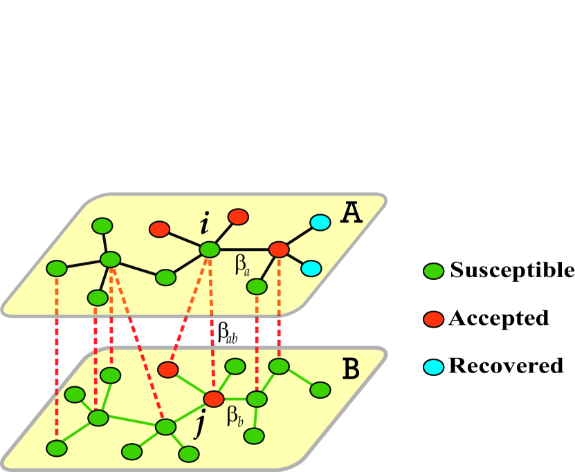
Figure 1: (Color online). Sketch of the Susceptible-Accepted-Recovered (SAR) model on a two-layered network. “Black”, “green” and “red” lines represent the links of the layer $\mathcal{A}$, $\mathcal{B}$ and the inter-layer $\mathcal{AB}$, respectively. $\beta_{a}$, $\beta_{b}$ and $\beta_{ab}$ denote the transmission probability of layers $\mathcal{A}$, $\mathcal{B}$ and $\mathcal{AB}$. At time $t$, the susceptible node $i$ in layer $\mathcal{A}$ may receive a piece of information from an accepted node in layer $\mathcal{A}$ and $\mathcal{B}$ with probability $\beta_{a}$ and $\beta_{ab}$, respectively. Once the node $i$ receives the information successfully from one accepted neighbor, the cumulative number $m$ of received information for node $i$ will increase $1$ and the accepted neighbor will not transmit the same information to the node $i$ any more. Assuming that the susceptible node $i$ has received the information $m$ times from the time step $0$ to $t$, the node $i$ will become accepted state if $m\geq T_{A}$.

To understand the effects of multiple channels in the information spreading process, we here introduce a two-layered network with coupling between its two layers, i.e. the layer $\mathcal{A}$ and $\mathcal{B}$ in Fig. 1. We let the two layers have the same size $N_{a}=N_{b}=N$ and their degree distributions $P_{A}(k)$ and $P_{B}(k)$ be different. We may imagine the layer $\mathcal{A}$ as a human communication network for one geographic region or community and the layer $\mathcal{B}$ for a separated region. There are two kinds of links for each node in the two-layered networks, i.e. intra-links within layer $\mathcal{A}$ or $\mathcal{B}$ and the inter-links between layer $\mathcal{A}$ and $\mathcal{B}$. Each node could receive information not only through friends, colleagues and family with intra-links in the same region, but also from distant relatives and friends with inter-links in another region by the telephone and Internet. In details, we firstly generate two separated networks $\mathcal{A}$ and $\mathcal{B}$ with the same size $N$ and different degree distributions $P_{A}(k_{a})$ and $P_{B}(k_{b})$, respectively. Then, we add links randomly between $\mathcal{A}$ and $\mathcal{B}$ until the steps we planned. The average node degrees of layer $\mathcal{A}$, $\mathcal{B}$ and inter-layer $\mathcal{AB}$ is presented by $\langle k_{a}\rangle$, $\langle k_{b}\rangle$, and $\langle k_{ab}\rangle$, respectively. In the above way, we obtain an uncorrelated two-layered network.

To discuss information spreading in the two-layered network, we adopt a Susceptible-Accepted-Recovered (SAR) model. At each time step, a node can occupy only one of the three states: (i) Susceptible: the node has not received the information yet or has received the information but hesitate to accept it; (ii) Accepted: the node accepts the information and transmits it to its neighbors; (iii) Recovered: the node loses interest to the information and will not spread it any more. Thus, this Susceptible-Accepted-Recovered (SAR) model is similar to the SIR (Susceptible-Infected-Refractory) model in epidemiology.

The information spreading process can be described as follows:

(i) At the beginning, a fraction $\rho_{0}$ of nodes are random uniformly chosen from the layer $\mathcal{A}$ as seeds (accepted state) to spread the first piece of information. All other nodes are in the susceptible state.

(ii) At each time step $t$, the susceptible node $i$ in layer $\mathcal{A}$ may receive a piece of information from an accepted node in layer $\mathcal{A}$ and $\mathcal{B}$ with probability $\beta_{a}$ and $\beta_{ab}$ (see Fig. 1), respectively. For the susceptible node in layer $\mathcal{B}$, the change of the nodes’ state is the same as in layer $\mathcal{A}$ but with probability $\beta_{b}$. Once the node $i$ receives the information successfully from an accepted neighbor, the cumulative number $m$ of received information for the node $i$ will increase one and this accepted neighbor will not transmit the same information to the node $i$ any more, i.e., non-redundant information transmission. As an individual has to remember the pieces of non-redundant information he or she received from neighbors before time $t$, the so-called non-redundant information memory is induced in our model.

(iii) When a susceptible node $i$ has received the information $m$ times until time step $t$ and $m\geq T_{A}$ in layer $\mathcal{A}$ (or $m\geq T_{B}$ in layer $\mathcal{B}$), the node $i$ will become accepted state, where $T_{A}$ and $T_{B}$ is the adoption threshold of node in layer $\mathcal{A}$ and $\mathcal{B}$, respectively. At the same time step, each accepted node will lose interest in transmitting the information and becomes recovered with probability $\mu$.

(iv) The steps are repeated until there is no accepted node in the network.

In our numerical simulations, we set the network size $N_{a}=N_{b}=10\,000$, recovered probability $\mu=1.0$, $\beta_{a}=\beta_{b}=\beta$, and initially chose $\rho_{0}=0.05$ of nodes in layer $\mathcal{A}$ to be accepted.

III theory

III.1 The edge-based compartmental theory on a single network

Let us first illustrate the edge-based compartmental theory for a single network, by following the methods introduced in Refs. Wang:2015 ; Volz:2008 ; Miller:2011 ; Shu:2016 ; Miller:2012 ; Miller:2013a ; Miller:2014 . We let $\rho_{S}(t)$, $\rho_{A}(t)$, and $\rho_{R}(t)$ be the densities of the Susceptible, Accepted, and Recovered nodes at time $t$, respectively. The spreading process will be ended when $t\rightarrow\infty$ and thus $\rho_{R}(\infty)$ represent the final fraction of accepted nodes.

We use a variable $\theta(t)$ to denote the probability that a node $v$ has not transmitted the information to the node $u$ along a randomly chosen edge by time $t$. For an uncorrelated, large and sparse network, the probability that a randomly chosen node $u$ of degree $k$ has received the information $m$ times from his/her neighbors at time $t$ is

$$\tau(k,m,\theta(t))=(_{m}^{k})\theta(t)^{k-m}(1-\theta(t))^{m}$$ (1)

Notice that a node with degree $k$ has the probability $1-\rho_{0}$ to be not one of the initial seeds. At the same time, the probability that a susceptible node $u$ with degree $k$ has received the information $m$ times and still does not accept it by time $t$ is $\sum_{m=0}^{T-1}\tau(k,m,\theta(t))$, where $T$ is the adoption threshold in the model. Combining the initial seeds and summing over all possible values of $m$, we obtain the probability that the node $u$ is still in the susceptible state at time $t$ as

$$s(k,t)=(1-\rho_{0})\sum_{m=0}^{T-1}\tau(k,m,\theta(t))$$ (2)

Averaging over all $k$, the density of susceptible nodes (i.e., the probability of a randomly chosen individual is in the susceptible state) at time $t$ is given by

$$\rho_{S}(t)=\sum\limits_{k=0}^{\infty}P(k)s(k,t).$$ (3)

where $P(k)$ is the degree distribution of the network. In order to solve $\rho_{S}(t)$, one needs to know $\theta(t)$. Since a neighbor $v$ of node $u$ may be susceptible, accepted, or recovered, $\theta(t)$ can be expressed as

$$\theta(t)=\Phi^{S}(t)+\Phi^{A}(t)+\Phi^{R}(t)$$ (4)

where $\Phi^{S}(t),\Phi^{A}(t),\Phi^{R}(t)$ is the probability that the neighbor $v$ is in the susceptible, accepted, recovery state, respectively, and has not transmitted the information to node $u$ through this connection. Once these three parameters derived, we will get the density of susceptible nodes at time $t$ by substituting them into Eq. (1)(2) and then into Eq. (3). For this purpose, in the following, we will focus on how to solve them.

To find $\Phi^{S}(t)$, we now consider a randomly chosen node $u$, and assume this node is in the cavity state, which means that it cannot transmit any information to its neighbors $v$ but can be informed by its neighbors. In this case, the neighbor $v$ can only get the information from its other neighbors except the node $u$. If a neighboring node $v$ of $u$ has degree $k^{\prime}$, the probability that node $v$ has received $m$ pieces of the information at time $t$ will be $\tau(k^{\prime}-1,m,\theta(t))=(_{m}^{k^{\prime}-1})\theta(t)^{k^{\prime}-1-m}(1-\theta(t))^{m}$. After received the information $m$ times, node $v$ still does not accept it with probability $(1-\rho_{0})\sum_{m=0}^{T-1}\tau(k^{\prime}-1,m,\theta(t))$. For uncorrelated networks, the probability that one edge from node $u$ connects with a node $v$ with degree $k^{\prime}$ is $k^{\prime}P(k^{\prime})/\langle k\rangle$, where $\langle k\rangle$ is the mean degree of the network. So, summing over all possible $k^{\prime}$, one obtains

$$\Phi^{S}(t)=(1-\rho_{0})\frac{\sum\limits_{k^{\prime}}k^{\prime}P(k^{\prime})\sum\limits_{m=0}^{T-1}\tau(k^{\prime}-1,m,\theta(t))}{\langle k\rangle}$$ (5)

The growth of $\Phi^{R}(t)$ includes two consecutive events: firstly, an accepted neighbor has not transmitted the information successfully to node $u$ with probability $1-\beta$; secondly, the accepted neighbor has become recovered with probability $\mu$. Combining these two events, the $\Phi^{A}(t)$ to $\Phi^{R}(t)$ flux is $\mu(1-\beta)\Phi^{A}(t)$. Thus, one gets

$$\frac{d\Phi^{R}(t)}{dt}=\mu(1-\beta)\Phi^{A}(t)$$ (6)

Once the accepted neighbor $v$ transmits the information to $u$ successfully (with probability $\beta$), the $\Phi^{A}(t)$ to $1-\theta(t)$ flux will be $\beta\Phi^{A}(t)$, which means

$$\frac{d(1-\theta(t))}{dt}=\beta\Phi^{A}(t).$$ (7)

That is

$$\frac{d\theta(t)}{dt}=-\beta\Phi^{A}(t).$$ (8)

Combining Eqs. (6) and (8) and considering (as initial conditions) $\theta(0)=1$ and $\Phi^{R}(0)=0$, one obtains

$$\Phi^{R}(t)=\frac{\mu[1-\theta(t)](1-\beta)}{\beta}.$$ (9)

Substituting Eqs. (5) and (9) into Eq.(4), we get an expression for $\Phi^{A}(t)$ in terms of $\theta(t)$. Then, one can rewrite Eq. (8) as

$$\frac{d\theta(t)}{dt} = -\beta\theta(t)+\mu(1-\theta(t))(1-\beta)$$ (10)

$$+\frac{\beta(1-\rho_{0})\sum_{k^{\prime}}k^{\prime}P(k^{\prime})\sum\limits_{m=0}^{T-1}\tau(k^{\prime}-1,m,\theta(t))}{\langle k\rangle}$$

With $\theta(t)$ on hand, the equation of the system comes out to be

$$\frac{d\rho_{R}(t)}{dt} = \mu\rho_{A}(t),$$

$$\rho_{S}(t) = \sum\limits_{k=0}^{\infty}P(k)s(k,t),$$

$$\rho_{A}(t) = 1-\rho_{S}(t)-\rho_{R}(t).$$ (11)

In fact, Eq. (10) does not depend on Eq. (III.1), so the system is governed by the single ordinary differential equation (10). Although the resulting equation are simpler than those found by other methods, it can be proven to exactly predict the disease/information spreading dynamics in the large-population limit for different network topologiesWang:2015 ; Volz:2008 ; Miller:2011 ; Shu:2016 ; Miller:2012 ; Miller:2013a ; Miller:2014 .

III.2 The edge-based compartmental theory on a two-layered network

Now, we develop an analogous theoretical framework from the single network to the case of two uncorrelated interconnected networks based on the approach in Refs. Zheng:2018 , which is suited to the problems studied in our work. In particular, when one assumes that the population is made up of two layers, then $P_{j}(k_{1},k_{2})$ denote the probability that a node of layer $j$ has $k_{1}$ degree in layer $1$ and $k_{2}$ in layer $2$. For the sake of simplicity, one can name the two layers $\mathcal{A}$ and $\mathcal{B}$ as $1$ and $2$. Let $\beta_{j,l}$ be the rate of transmission across an edge from network $l$ to network $j$, and let us define $\mu$ to be the recovery rate of a node in any layer.

Firstly, let us define $\theta_{j,l}$ to be the probability that randomly chosen an edge $(u,v)$, node $v$ in layer $j$ ($j=1,2$) has not transmitted the information to the node $u$ in layer $l$ ($l=1,2$) by time $t$. For the considered case, we have $\theta_{1,2}$, $\theta_{1,1}$, $\theta_{2,1}$ and $\theta_{2,2}$ four variables. Once the four variables were obtained, we can solve the equations of the system.

Now, we will solve $\theta_{1,2}$ as an example in detail. Similarly to the the case of single network, a neighbor $v$ in layer 2 of node $u$ in layer 1 may be susceptible, accepted, or recovered. Then $\theta_{1,2}$ can be expressed as

$$\theta_{1,2}=\Phi^{S}_{1,2}+\Phi^{A}_{1,2}+\Phi^{R}_{1,2}$$ (12)

where $\Phi^{S}_{1,2}$, $\Phi^{A}_{1,2}$, $\Phi^{R}_{1,2}$ is the probability that the neighbor $v$ is in the susceptible, accepted, recovery state, and has not transmitted the information to node $u$ through this edge $(u,v)$.

Similarly, to find $\Phi^{S}_{1,2}$, the neighbor $v$ in layer 2 can only get the information from its other neighbors except the node $u$ in layer 1. Thus, the probability that the node $v$ with degree $(k_{1},k_{2})$ has received the information $m$ times from his/her neighbors at time $t$ is $\tau(k_{1}-1,n,\theta_{2,1})\tau(k_{2},m-n,\theta_{2,2})$, where $\tau(k_{1}-1,n,\theta_{2,1})$ indicates the probability that the node $v$ received $n$ times information from $k_{1}-1$ neighbors with $\theta_{2,1}$ and $\tau(k_{2},m-n,\theta_{2,2})$ is the probability that the node $v$ received the last $m-n$ times information from $k_{2}$ neighbors with $\theta_{2,2}$. It should be noted that function $\tau(k,m,\theta)=(_{m}^{k})\theta^{k-m}(1-\theta)^{m}$, which has the similar expression as Eq. (1). After received the information $m$ times, node $v$ still does not accept it with probability

$$X_{1,2}=\sum\limits_{m=0}^{T_{B}-1}\sum\limits_{n=0}^{m}\tau(k_{1}-1,n,\theta_{2,1})\tau(k_{2},m-n,\theta_{2,2})$$ (13)

For uncorrelated networks, the probability that one edge from node $u$ connects with a node $v$ with degree $(k_{1},k_{2})$ is $\frac{k_{1}P_{2}(k_{1},k_{2})}{\sum_{k_{1},k_{2}}k_{1}P_{2}(k_{1},k_{2})}$. Thus, one has

$$\Phi^{S}_{1,2} = \frac{\sum\limits_{k_{1},k_{2}}k_{1}P_{2}(k_{1},k_{2})X_{1,2}}{\sum\limits_{k_{1},k_{2}}k_{1}P_{2}(k_{1},k_{2})}$$ (14)

It is easily to know that the growth of $\Phi^{R}_{1,2}$ includes two consecutive events: first, an accepted neighbor has not transmitted the information to node $u$ via with probability $1-\theta_{1,2}$; second, the accepted neighbor has been recovered with probability $\mu$. Combining these two events, the $\Phi^{A}_{1,2}$ to $\Phi^{R}_{1,2}$ flux is $\mu(1-\theta_{1,2})\Phi^{A}_{1,2}$. Thus, one gets

$$\frac{d\Phi^{R}_{1,2}}{dt} = \mu(1-\theta_{1,2})\Phi^{A}_{1,2}$$ (15)

Once the accepted neighbor $v$ in layer 2 transmits the information to node $u$ in layer 1 successfully (with probability $\beta_{1,2}$), the $\Phi^{A}_{1,2}$ to $1-\theta_{1,2}$ flux will be $\beta_{1,2}\Phi^{A}_{1,2}$, which means

$$\frac{d\theta_{1,2}}{dt} = -\beta_{1,2}\Phi^{A}_{1,2}$$ (16)

Combining Eqs. (15) and (16), and considering the initial conditions $\theta_{1,2}(0)=1$ and $\Phi^{R}_{1,2}(0)=0$, one obtains

$$\Phi^{R}_{1,2} = \frac{\mu(1-\theta_{1,2})(1-\beta_{1,2})}{\beta_{1,2}}$$ (17)

Substituting Eqs. (14) (17) into Eq.(12) and then into (16) , one gets

$$\dot{\theta}_{1,2} = -\beta_{1,2}(\theta_{1,2}-\Phi^{S}_{1,2}-\Phi^{R}_{1,2})$$ (18)

$$= -\beta_{1,2}\theta_{1,2}+\mu(1-\theta_{1,2})(1-\beta_{1,2})$$

$$+\beta_{1,2}\frac{\sum\limits_{k_{1},k_{2}}k_{1}P_{2}(k_{1},k_{2})X_{1,2}}{\sum\limits_{k_{1},k_{2}}k_{1}P_{2}(k_{1},k_{2})}$$

Similarly, one can write down $\theta_{1,1}$, $\theta_{2,1}$ and $\theta_{2,2}$ as follows

$$\dot{\theta}_{1,1} = -\beta_{1,1}(\theta_{1,1}-\Phi^{S}_{1,1}-\Phi^{R}_{1,1})$$ (19)

$$= -\beta_{1,1}\theta_{1,1}+\mu(1-\theta_{1,1})(1-\beta_{1,1})$$

$$+\beta_{1,1}\frac{(1-\rho_{0})\sum\limits_{k_{1},k_{2}}k_{1}P_{1}(k_{1},k_{2})X_{1,1}}{\sum\limits_{k_{1},k_{2}}k_{1}P_{1}(k_{1},k_{2})}$$

$$\dot{\theta}_{2,1} = \!-\beta_{2,1}(\theta_{2,1}-\Phi^{S}_{2,1}-\Phi^{R}_{2,1})$$ (20)

$$= -\beta_{2,1}\theta_{2,1}+\mu(1-\theta_{2,1})(1-\beta_{2,1})$$

$$+\beta_{2,1}\frac{(1-\rho_{0})\sum\limits_{k_{1},k_{2}}k_{2}P_{1}(k_{1},k_{2})X_{2,1}}{\sum\limits_{k_{1},k_{2}}k_{2}P_{1}(k_{1},k_{2})}$$

$$\dot{\theta}_{2,2} = -\beta_{2,2}(\theta_{2,2}-\Phi^{S}_{2,2}-\Phi^{R}_{2,2})$$ (21)

$$= -\beta_{2,2}\theta_{2,2}+\mu(1-\theta_{2,2})(1-\beta_{2,2})$$

$$+\beta_{2,2}\frac{\sum\limits_{k_{1},k_{2}}k_{2}P_{2}(k_{1},k_{2})X_{2,2}}{\sum\limits_{k_{1},k_{2}}k_{2}P_{2}(k_{1},k_{2})}$$

where

$$X_{1,1} = \sum\limits_{m=0}^{T_{A}-1}\sum\limits_{n=0}^{m}\tau(k_{1}-1,n,\theta_{1,1})\tau(k_{2},m-n,\theta_{1,2})$$ (22)

$$X_{2,1} = \sum\limits_{m=0}^{T_{A}-1}\sum\limits_{n=0}^{m}\tau(k_{1},n,\theta_{1,1})\tau(k_{2}-1,m-n,\theta_{1,2})$$ (23)

$$X_{2,2} = \sum\limits_{m=0}^{T_{B}-1}\sum\limits_{n=0}^{m}\tau(k_{1},n,\theta_{2,1})\tau(k_{2}-1,m-n,\theta_{2,2})$$ (24)

It should be noted that as a node in layer $1$ has the probability $1-\rho_{0}$ not to be one of the initial seeds, after received the information $m$ times, node $v$ through a corresponding edge still does not accept it with probability $(1-\rho_{0})X_{1,1}$ and $(1-\rho_{0})X_{2,1}$ in Eqs. (19) and (20), respectively. With Eqs. (18-24) on hand, the densities associated with each distinct state can be obtained by

$$\begin{cases}\dot{R}_{1}=\mu A_{1}(t)\\ S_{1}(t)=(1-\rho_{0})\sum\limits_{k_{1},k_{2}}^{\infty}P_{1}(k_{1},k_{2})Y_{1}\\ A_{1}(t)=1-S_{1}(t)-R_{1}(t)\end{cases}$$ (25)

$$\begin{cases}\dot{R}_{2}=\mu A_{2}(t)\\ S_{2}(t)=\sum\limits_{k_{1},k_{2}}^{\infty}P_{2}(k_{1},k_{2})Y_{2}\\ A_{2}(t)=1-S_{2}(t)-R_{2}(t)\end{cases}$$ (26)

where

$$Y_{1}=\sum\limits_{m=0}^{T_{A}-1}\sum\limits_{n=0}^{m}\tau(k_{1},n,\theta_{1,1})\tau(k_{2},m-n,\theta_{1,2})$$ (27)

$$Y_{2}=\sum\limits_{m=0}^{T_{B}-1}\sum\limits_{n=0}^{m}\tau(k_{1},n,\theta_{2,1})\tau(k_{2},m-n,\theta_{2,2})$$ (28)

Eqs. (25) and (26) are the main theoretical results in this paper. To obtain the densities associated with each state, instead of getting the analytic solutions of Eqs. (25) and (26), we solve them by numerical integration and get the corresponding theoretical curves.

IV Results

To study the effects of multiple channels on information spreading, we have performed extensive simulations with our model in coupled Scale-free (SF)Catanzaro:2005 and Erdos-Re̋nyi (ER) networks Albert:2002 . To compare the theoretical predictions with the numerical results, we also take into account coupled ER-ER and SF-SF networks in this work. Next, we mainly try to find out the key factors, which influence the emergence of the double transition on information spreading process.

IV.1 The effects of multiple channels on the double transition

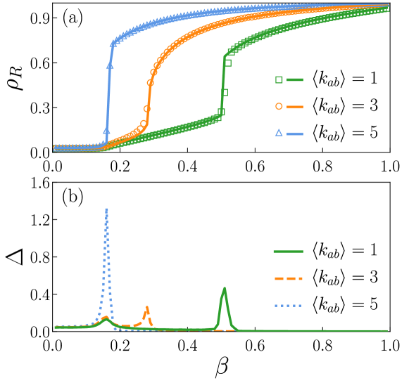
Figure 2: (Color online). Emergence of the double transition on information spreading process on SF-ER networks. (a) and (b) represent the density of final recovered nodes $\rho_{R}$ and variability $\Delta$ as a function of transmission probability $\beta$ with different average degree $\langle k_{ab}\rangle$, respectively. Squares, circles and up triangles represent $\langle k_{ab}\rangle=1$, $3$ and $5$, respectively. The symbols show the simulated results and the lines are the corresponding theoretical results in (a) from Eqs. (25) and (26). The results are averaged over $10^{3}$ independent realizations. The parameters are $N_{a}=N_{b}=10\,000$, $\mu=1.0$, $\beta_{ab}=0.5$, $T_{A}=T_{B}=2$, $\rho_{0}=0.05$, $P_{A}(k_{a})\sim k_{a}^{-2.1}$, $\langle k_{a}\rangle=6$, $\langle k_{b}\rangle=6$.

To better quantify the spreading behavior, we let $\rho_{S}(t)$, $\rho_{A}(t)$ and $\rho_{R}(t)$ denote the fraction of susceptible, accepted and recovered nodes at time $t$ in the whole network. When the spreading is ended, the final size of recovered nodes can be denoted by $\rho_{R}$. A larger $\rho_{R}$ implies a larger spreading range at the final state. To numerically identify the effective spreading threshold $\beta_{c}$ of the SAR model, we use the variability measureShu:2016 ; Crepey:2015 :

$$\Delta=\frac{\sqrt{\langle\rho_{R}^{2}\rangle-\langle\rho_{R}\rangle^{2}}}{\langle\rho_{R}\rangle}$$ (29)

In general, the variability $\Delta$ exhibits a peak at a critical pointShu:2016 ; Crepey:2015 . Thus, we estimate the numerical effective spreading threshold $\beta_{c}$ from the position of the peak of the variability.

Fig. 2(a) shows the final size of recovered nodes $\rho_{R}$ as a function of transmission probability $\beta$ with different average degree $\langle k_{ab}\rangle$ on SF-ER networks. Fig. 2(b) shows the variability $\Delta$ versus $\beta$ with corresponding $\langle k_{ab}\rangle$ in Fig. 2(a). When the interaction strength is weak (i.e., $\langle k_{ab}\rangle$ is relatively small), the double transition occur on the information spreading process, which is indicated by two peaks of $\Delta$ in Fig. 2(b). It has also found that the system undergoes a continuous transition from accepted free phase to accepted phase and a following discontinuous transition between the accepted phases. In addition, with the increasing of $\langle k_{ab}\rangle$, the second critical point $\beta_{c}^{2}$ close to the first one $\beta_{c}^{1}$. Once the coupling strength is strong enough ($\langle k_{ab}\rangle=5$), the two critical points merge into one, i.e., the second transition is vanished. These result have been confirmed by Eqs. (25) and (26) of the theory, see the lines in Fig. 2(a). It is maybe helpful to understand the influence of $\langle k_{ab}\rangle$ on the double transition from the aspect of purely coupling in network structure. When the coupling strength is strong, a two-layered network behave as a solid single network Radicchi:2013 ; Sahneh:2015 . In this case, the effect of multiple channels is not prominent and the spreading behavior is the same as the common one Wang:2015 . Therefore, a key factor determining the occurrence of double transition is a weak coupling between two networks.

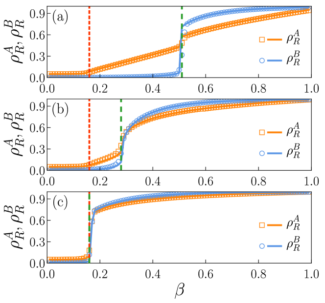
Figure 3: (Color online). The densities of final recovered nodes $\rho_{R}^{A}$ and $\rho_{R}^{B}$ in layer $\mathcal{A}$ and $\mathcal{B}$ as a function of transmission probability $\beta$, where (a), (b) and (c) represent the cases of average degree $\langle k_{ab}\rangle=1$, $\langle k_{ab}\rangle=3$, and $\langle k_{ab}\rangle=5$, respectively. Based on the peaks of $\Delta$ in Fig. 2(b), the red and green dash lines indicate the first and second critical point, respectively. The symbols show the simulated results and the solid lines are the corresponding theoretical results. All the parameters are set as Fig. 2.

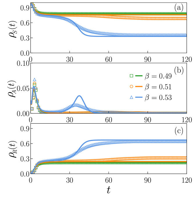
Figure 4: (Color online). Average densities of (a) susceptible $\rho_{S}(t)$, (b) accepted $\rho_{A}(t)$, and (c) recovered $\rho_{R}(t)$ nodes versus time $t$ with different transmission probability $\beta$. Squares, circles and up triangles represent $\beta=0.49$, $0.51$ and $0.53$, respectively, which indicate the spreading patterns below, at and above the second transition in Fig. 2(a) with $\langle k_{ab}\rangle=1$. The symbols show the simulated results and the lines are the corresponding theoretical results. All the results are averaged over $100$ independent realizations and the parameters are the same as Fig. 2.

To gather a deeper understanding the double transition phenomenon, in Fig. 3 we also measure the densities of final recovered nodes $\rho_{R}^{A}$ and $\rho_{R}^{B}$ in the layer $\mathcal{A}$ and $\mathcal{B}$ as a function of transmission probability $\beta$, where Fig. 3(a), (b) and (c) report the cases of average degree $\langle k_{ab}\rangle=1$, $\langle k_{ab}\rangle=3$, and $\langle k_{ab}\rangle=5$, respectively. Based on the peaks of $\Delta$ in Fig. 2(b), the red and green dash lines indicate the first and second critical point $\beta_{c}^{1}$ and $\beta_{c}^{2}$, respectively. Comparing with Fig. 3(a), (b) and (c), it is visible to observe that the first threshold $\beta_{c}^{1}$ is the same, indicating that the first critical point $\beta_{c}^{1}$ corresponds to the spreading threshold in layer $\mathcal{A}$. With the increase of $\beta$, more and more individuals have accepted the information in layer $\mathcal{A}$ and more information has been spread to layer $\mathcal{B}$. When the $\beta$ closes to the second threshold $\beta_{c}^{2}$, the system undergoes an abrupt transition. For a very strong coupling (see Fig. 3(c)), the two critical points merge into one, which shows a discontinues transition as the traditional threshold model Dodds:2004 ; Wang:2015 . In addition, from Fig. 3(a) and (b), it is found that when $\beta_{c}^{1}<\beta<\beta_{c}^{2}$, the density of recovered nodes in layer $\mathcal{B}$ is not zero, indicating the information has been spread to a small fraction individuals in layer $\mathcal{B}$ but these small part accepted individuals are unable to trigger an outbreak of the information.

To better understand the spreading behavior around the second threshold $\beta_{c}^{2}$, we study the evolution of the nodes densities of susceptible $\rho_{S}(t)$, accepted $\rho_{A}(t)$, and recovered $\rho_{R}(t)$ in Fig. 4, respectively. The green, yellow and blue symbols and lines represent the spreading cases of below, at and above the second critical point $\beta_{c}^{2}$, respectively. It is apparent to observe that when $\beta>\beta_{c}^{2}$ (see the blue symbols and lines), $\rho_{A}(t)$ shows two peaks in Fig. 4(b) and $\rho_{R}(t)$ increases dramatically at the final stage in Fig. 4(c), implying that the system undergoes a second outbreak.

IV.2 The effects of the adoption threshold $T_{A}$ and $T_{B}$

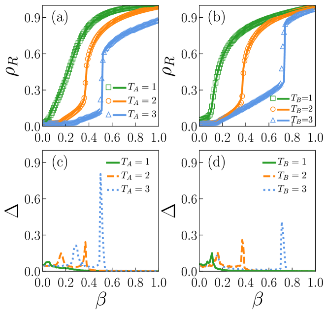
Figure 5: (Color online). The effects of the adoption threshold $T_{A}$ and $T_{B}$ on double transition. (a) and (b) show the dependence of the final recovered density $\rho_{R}$ on the transmission probability $\beta$ with different $T_{A}$ and $T_{B}$, respectively. (c) and (d) plot the corresponding variability $\Delta$ in the case of (a) and (b), respectively. The green, yellow and blue symbols and lines represent $T_{A}=1$, $2$, $3$ in (a)(c) and $T_{B}=1$, $2$, $3$ in (b)(d), respectively, where the symbols represent the simulated results and the lines are the corresponding theoretical results in (a) and (b) from Eqs. (25) and (26). The parameters are set as $T_{B}=2$ in (a) and $T_{A}=2$ in (b). The other ones are $N_{a}=N_{b}=10\,000$, $\mu=1.0$, $\beta_{ab}=0.5$, $\langle k_{ab}\rangle=2$, $\rho_{0}=0.05$, $P_{A}(k_{a})\sim k_{a}^{-2.1}$, $\langle k_{a}\rangle=6$, $\langle k_{b}\rangle=6$.

In general, the adoption threshold of the individuals will influence the phase transition on the spreading dynamicsDodds:2004 ; Wang:2015 . In this sense, we next study the effects of the adoption threshold $T_{A}$ and $T_{B}$ on the double transition. Fig. 5(a) and (b) show the dependence of the final recovered density $\rho_{R}$ on the transmission probability $\beta$ with typical $T_{A}$ and $T_{B}$, respectively. As is shown in Fig. 5(a), when $T_{A}=1$, the phenomenon of double transition do not occur in the spreading process. The corresponding variability $\Delta$ clearly confirms this point in Fig. 5(c). When $T_{A}=2$ and $T_{A}=3$, it is observed that the double transition emerge with the increasing of $\beta$. The corresponding variability $\Delta$ shows two peaks in Fig. 5(c). Similarly, in Fig. 5(b) and (d), we plot the final recovered density $\rho_{R}$ and the corresponding variability $\Delta$ as a function of transmission probability $\beta$ with different $T_{B}$, respectively. The results are similar to the case in Fig. 5(a) and (c). It is obvious to know that increasing the adoption threshold impedes individuals from accepting the information. A larger value of adoption threshold means that the individual will accept the information only it receives the information more times from distinct neighbors. As a result, the individuals easily accept the information when the adoption threshold is small (i.e., $T_{A}=1$ or $T_{B}=1$). Particularly, when $T_{A}=1$, the information is spread fast in layer $\mathcal{A}$ and then the individuals in layer $\mathcal{B}$ know the information quickly. Thus we observe a macroscopic outbreak at the same time. While for the case of $T_{B}=1$, the individuals in layer $\mathcal{B}$ will accept the information once they received it one time. In this case, the information in layer $\mathcal{A}$ can spill into layer $\mathcal{B}$ easily and it is equivalent to a relatively strong interaction between the two layers, where the spreading process shows a synchronous outbreak behavior. Therefore, the double transition disappears in this situation.

IV.3 Influence of network structure

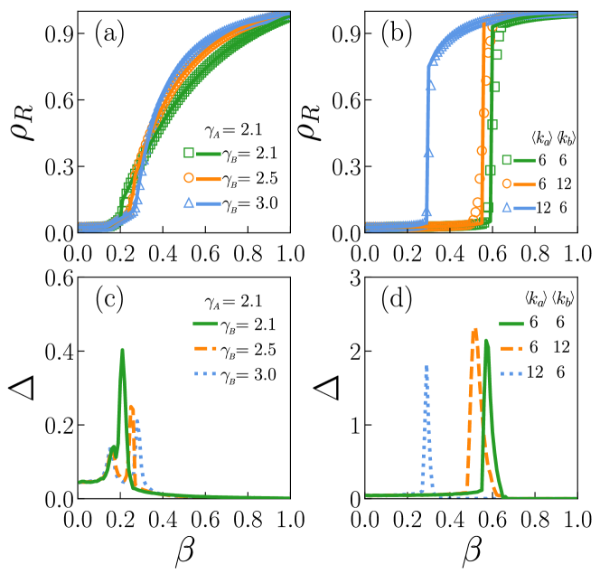
Figure 6: (Color online). The influence of network structure on double transition. (a) and (c) show $\rho_{R}$ and $\Delta$ versus $\beta$ with different degree exponent $\gamma_{B}$ in coupled SF-SF networks, respectively. (b) and (d) show $\rho_{R}$ and $\Delta$ versus $\beta$ with different $\langle k_{a}\rangle$ and $\langle k_{b}\rangle$ in coupled ER-ER networks, respectively. The degree exponent $\gamma_{A}=2.1$ is fixed in (a) and (c) and the other parameters are set as $\langle k_{ab}\rangle=2$, $T_{A}=T_{B}=2$, $N_{a}=N_{b}=10\,000$, $\mu=1.0$, $\beta_{ab}=0.5$, $\rho_{0}=0.05$.

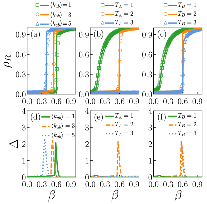
Figure 7: (Color online). The double transition disappears on coupled ER-ER networks. The dependence of the final recovered density $\rho_{R}$ on the transmission probability $\beta$ with different (a)$\langle k_{ab}\rangle$, (b) $T_{A}$ and (c) $T_{B}$, respectively. (d) (e) and (f) plot the corresponding variability $\Delta$ in the case of (a) (b) and (c), respectively. The parameters are set as $T_{A}=T_{B}=2$ in (a)(d); $T_{B}=2$ in (b)(e); $T_{A}=2$ in (c)(f), respectively. The other ones are $\langle k_{a}\rangle=\langle k_{b}\rangle=6$, $\langle k_{ab}\rangle=2$, $N_{a}=N_{b}=10\,000$, $\mu=1.0$, $\beta_{ab}=0.5$, $\rho_{0}=0.05$.

One more key question is how the network topology affects the phenomenon of the double transition. To answer this question, we consider the influence of degree distribution of coupled SF-SF and ER-ER networks. Notice that the coupled SF-SF network is generated with the power-law degree distribution $P_{A}(k_{a})\sim k_{a}^{-\gamma_{A}}$ and $P_{B}(k_{b})\sim k_{b}^{-\gamma_{B}}$ in layer $\mathcal{A}$ and $\mathcal{B}$, respectively, where $\gamma_{A}$ and $\gamma_{B}$ are the degree exponents. The smaller of the degree exponent is, the stronger of the heterogeneity of network structure will be. For fixed $\gamma_{A}=2.1$, Fig. 6 (a) and (c) show $\rho_{R}$ and $\Delta$ versus $\beta$ with different degree exponent $\gamma_{B}$ in coupled SF-SF networks, respectively. It is found that when the $\gamma_{B}$ closes to $\gamma_{A}$, the phenomenon of the double transition is not prominent any more. As the difference of the heterogeneity in degree distribution between the two layers is not distinctive, the spreading speed in layer $\mathcal{A}$ and $\mathcal{B}$ are comparative. In this case, it is easy to observe the synchronous outbreak behavior between layer $\mathcal{A}$ and $\mathcal{B}$. In fact, the result can be qualitatively explained as followsWang:2015 : From our model, we know that hubs accept the information with more larger probability. With the increasing of network heterogeneity in layer $\mathcal{B}$, the network has a large number of nodes with very small degrees and more nodes with large degrees. At the beginning, the hubs facilitate the information spreading as they are more likely to receive the information from layer $\mathcal{A}$. After that, a large number of nodes in layer $\mathcal{B}$ with very small degrees will accept the information, resulting a similar behavior as layer $\mathcal{A}$ in the spreading process.

To deeply understand this point, we investigate a specific case with the same degree distribution in coupled ER-ER networks. As is shown in Fig. 6(b) and (d), both the curves of $\rho_{R}$ and $\Delta$ indicate that the double transition disappears with different $\langle k_{a}\rangle$ and $\langle k_{b}\rangle$. What is more, for different cases of $\langle k_{ab}\rangle$, $T_{A}$ and $T_{B}$, the disappearance of the double transition is also found in Fig. 7. In an ER network, the individuals are more likely to accept or not accept the information synchronously, which result in a discontinuous transition Wang:2015 . These results confirm again that the heterogeneity of degree distribution in each layer is very helpful for the appearance of the double transition.

V Conclusions

In recent years, researchers found that under certain conditions, there exists a double transition in the infected fraction versus the transmission probability on the epidemic spreading process. However, it is not clear whether it exists in the information spreading dynamics as the information spreading carries its special features, such as the effects of multiple channels, memory effects and non-redundant contacts etc. By combining these key factors in the information spreading dynamics, we indeed find the double transition in the phase diagram. These special features play a crucial role on the appearance of the double transition.

In summary, we have proposed a SAR model to describe the information spreading process on a two-layered network, where we emphasize the effects of multiple channels, memory and non-redundant contacts. Our simulation results show that there is a double transition in the phase diagram. Moreover, we find that such a phenomenon originates from two outbreaks between the two networks, which is a distinctive feature of a multilayer network of interactions. Further, we reveal that the double transition are driven by a weak coupling condition between the two layers, a large adoption threshold and the difference of the degree distributions betwen the two networks. An edge-based compartmental theory is developed which fully explains all numerical results. Our findings may be helpful for understanding the secondary outbreaks of the information in our life.

VI Acknowledgements

This work was partially supported by the NNSF of China under Grant No. 11505114 and No. 10975099, the Program for Professor of Special Appointment (Orientational Scholar) at Shanghai Institutions of Higher Learning under Grants No. QD2015016, and the Fundamental Research Funds for the central Universities under Grants No. YJ201830.

VII References

References

- (1) R. Pastor-Satorras and A. Vespignani, Phys. Rev. Lett. 86, 3200 (2001).
- (2) M. Boguna and R. Pastor-Satorras, Phys. Rev. E 66, 047104 (2002).
- (3) S. C. Ferreira, C. Castellano and R. Pastor-Satorras, Phys. Rev. E 86, 041125 (2012).
- (4) M. Boguna, C. Castellano and R. Pastor-Satorras, Phys. Rev. Lett. 111, 068701 (2013).
- (5) R. Parshani, S. Carmi, and S. Havlin, Phys. Rev. Lett. 104, 258701 (2010).
- (6) C. Castellano and R. Pastor-Satorras, Phys. Rev. Lett. 105, 218701 (2010).
- (7) V. Colizza, R. Pastor-Satorras and A. Vespignani, Nature Phys. 3, 276-282 (2007).
- (8) V. Colizza and A. Vespignani, Phys. Rev. Lett. 99, 148701 (2007).
- (9) A. Baronchelli, M. Catanzaro and R. Pastor-Satorras, Phys. Rev. E 78, 016111 (2008).
- (10) M. Tang, L. Liu and Z. Liu, Phys. Rev. E 79, 016108 (2009).
- (11) S. Boccaletti, G. Bianconi, R. Criado, C. I. del Genio, J. Gómez-Gardeñes, M. Romance, I. Sendiña-Nadal, Z. Wang, and M. Zanin, Phys. Rep. 544, 1 (2014).
- (12) L. Feng, C. P. Monterola, and Y. Hu, New J. Phys. 17(6), 063025 (2015).
- (13) F. D. Sahneh, C. Scoglio, and F. N. Chowdhury, In 2013 American Control Conference (pp. 2307-2312). IEEE (2013).
- (14) H. Wang, Q. Li, G. D’Agostino, S. Havlin, H. E. Stanley, and P. Van Mieghem, Phys. Rev. E 88(2), 022801 (2013).
- (15) O. Yagan, D. Qian, J. Zhang, and D. Cochran, IEEE J. Sel. Areas Commun. 31(6), 1038-1048 (2013).
- (16) M. E. Newman, Phys. Rev. Lett. 95(10), 108701 (2005).
- (17) V. Marceau, P. A. Noël, L. Hébert-Dufresne, A. Allard, and L. J. Dubé, Phys. Rev. E 84, 026105 (2011).
- (18) C. Buono, and L. A. Braunstein, Europhy. Lett. 109(2), 26001 (2015).
- (19) C. Buono, L. G. Alvarez-Zuzek, P. A. Macri, and L. A. Braunstein, PloS One 9(3), e92200 (2014).
- (20) Y. Zhao, M. Zheng and Z. Liu, Chaos 24, 043129 (2014).
- (21) M. Zheng, M. Zhao, B. Min, and Z. Liu, Sci. Rep., 7, 2424 (2017).
- (22) M. Zheng, W. Wang, M. Tang, J. Zhou, S. Boccaletti, and Z. Liu, Chaos, Solitons & Fractals, 107 (2018) 135-142.
- (23) P. Holme and J. Saramaki, Phys. Rep. 519, 97-125 (2012).
- (24) N. Perra, B. Goncalves, R. Pastor-Satorras and A. Vespignani, Sci. Rep. 2, 469 (2012).
- (25) R. Pastor-Satorras, C. Castellano, P. V. Mieghem and A. Vespignani, Rev. Mod. Phys. 87, 925 (2015).
- (26) A. Barrat, M. Barthelemy, and A. Vespignani, Dynamical Processes on Complex Networks (Cambridge University Press, Cambridge, England, 2008).
- (27) S. N. Dorogovtsev, A. V. Goltsev, and J. F. F. Mendes, Rev. Mod. Phys. 80, 1275 (2008).
- (28) W. Wang, M. Tang, H. E. Stanley, and L. A. Braunstein, Rep. Prog. Phys., 80(3), 036603 (2017).
- (29) P. Colomer-de Simon , M. Boguñá , Phys. Rev. X 4, 041020 (2014).
- (30) U. Bhat, M. Shrestha, L. Hébert-Dufresne, Phys. Rev. E 95, 012314 (2017).
- (31) A. Allard, B. M. Althouse, S. V. Scarpino, and L. Hébert-Dufresne, Proc. Natl. Acad. Sci. USA 114(34), 8969-8973 (2017).
- (32) B. Min, and M. S. Miguel, arXiv:1712.05059 (2017).
- (33) P. S. Dodds, and D. J. Watts, Phys. Rev. Lett. 92 218701 (2004).
- (34) L. Lü, D.-B. Chen, T. Zhou, New J. Phys. 13, 123005 (2011).
- (35) M. Zheng, L. Lü, and M. Zhao, Phys. Rev. E 88(1), 012818 (2013).
- (36) W. Wang, M. Tang, H. F. Zhang, and Y. C. Lai, Phys. Rev. E 92, 012820 (2015).
- (37) J. Wu, M. Zheng, Z. K. Zhang, W. Wang, C. Gu, and Z. Liu, Chaos 28(3), 033113 (2018).
- (38) C. D. Brummitt, K. M. Lee, and K. I. Goh, Phys. Rev. E 85(4), 045102 (2012).
- (39) K. M. Lee, C. D. Brummitt, and K. I. Goh, Phys. Rev. E 90(6), 062816 (2014).
- (40) B. Min, S. H. Gwak, N. Lee, and K. I. Goh, Sci. Rep. 6, 21392 (2016).
- (41) S. Funk, and V. A. Jansen, Phys. Rev. E 81, 036118 (2010).
- (42) A. Allard, P. A. Noël, L. J. Dubé, and B. Pourbohloul, Phys. Rev. E 79, 036113 (2009).
- (43) S. W. Son, G. Bizhani, C. Christensen, P. Grassberger, and M. Paczuski, Europhy. Lett. 97, 16006 (2012).
- (44) J. Sanz, C. Y. Xia, S. Meloni, and Y. Moreno, Phys. Rev. X 4, 041005 (2014).
- (45) E. A. Leicht, and R. M. D’Souza, arXiv:0907.0894 (2009).
- (46) A. Hackett, D. Cellai, S. Gómez, A. Arenas, and J. P. Gleeson, Phys. Rev. X 6(2), 021002 (2016).
- (47) M. Dickison, S. Havlin, and H. E. Stanley, Phys. Rev. E 85, 066109 (2012).
- (48) A. Saumell-Mendiola, M. A. Serrano, and M. Boguñá, Phys. Rev. E 86, 026106 (2012).
- (49) E. Volz, J. Math. Biol 56(3), 293-310 (2008).
- (50) J. C. Miller, J. Math. Biol. 62(3), 349-358 (2011).
- (51) P. Shu, W. Wang, M. Tang, P. Zhao, and Y. C. Zhang, Chaos 26(6), 063108 (2016).
- (52) J. C. Miller, A. C. Slim, and E. M. Volz, J. R. Soc. Interface 9(70), 890-906 (2012).
- (53) J. C. Miller, and E. M. Volz, PloS One 8(8), e69162 (2013).
- (54) J. C. Miller, PloS one 9(7), e101421 (2014).
- (55) M. Catanzaro, M. Boguñá, and R. Pastor-Satorras, Phys. Rev. E 71, 027103 (2005).
- (56) R. Albert, and A.-L. Barabási, Rev. Mod. Phys. 74, 47-97 (2002).
- (57) P. Crépey, F. P. Alvarez, and M. Barthélemy, Phys. Rev. E 73, 046131 (2006).
- (58) F. Radicchi, and A.Arenas, Nat. Phys. 9(11), 717-720 (2013).
- (59) F. D. Sahneh, C. Scoglio, and P. Van Mieghem, Phys. Rev. E 92(4), 040801 (2015).