Self-diffusion coefficient of the square-well fluid from molecular dynamics within the constant force approach

Abstract

We present a systematic study of the self-diffusion coefficient for a fluid of particles interacting via the square-well pair potential by means of molecular dynamics simulations in the canonical $(N,V,T)$ ensemble. The discrete nature of the interaction potential is modeled through the constant force approximation and the self-diffusion coefficient is determined for several packing fractions at super critical thermodynamic states. The dependence of the self-diffusion coefficient with the potential range $\lambda$ is analyzed in the range of $1.1\leq\lambda\leq 1.5$. The obtained molecular dynamics simulations results are in agreement with the self-diffusion coefficient predicted with the Enskog method. Additionally, we show that diffusion coefficient is very sensitive to the potential range, $\lambda$, at low densities leading to a density dependence of this coefficient not shared with other macroscopic properties such as the equation of state. The constant force approximation used in this work to model the discrete pair potentials has shown to be an excellent scheme to compute transport properties using standard computer simulations. Finally, the simulation results presented here are resourceful to improving theoretical approaches, such as the Enskog method.

I Introduction

The square-well (SW) pair potential has been widely used in statistical mechanics in both theoretical approaches Barker1967 ; Smith1970 ; Smith1971 ; Henderson1976 ; Henderson1980 ; Carley1977 ; Carley1981 ; Carley1983 ; DelRio1983 ; DelRio1985 ; DelRio1987 ; DelRio1987v2 ; DelRio1989 ; DelRio1991 ; Gil1996 and computer simulations schemes Rotenberg1965 ; Lado1968 ; Rosenfeld1975 ; Scarfe1976 ; Vega1992 . This simple model has a repulsive and an attractive contribution, thus, the main feature of this potential is the ability to control, independently, the energy and range interaction between molecules Paschinger2005 , this feature gives us the opportunity to characterize different systems of interest, ranging from simple liquids to complex fluids Alejandro1997 and even colloidal suspensions Duda2009 . Many of those fluids are being direct analogies of real substances. Thus, nowadays, the SW fluid is used to gain insight about the thermodynamics and phase behavior of ideal and real fluids Clare1999 ; Clare2010 .

However, results about transport properties of the SW pair potential are scarce, this lack of information is mainly due to the technical issues with dealing, in a dynamical way, with non-continuous potentials. In general, the transport properties are of interest in academic and industrial areas, e.g., for the design or manipulation of processes where not only the initial and final state of the system are of interest, furthermore, a complete thermodynamic description requires detail information about how the system goes from a steady state to another one, i.e., how a perturbation acts over an equilibrium state. In particular, one of the most relevant transport properties to characterize the mass transfer is the diffusion coefficient. This coefficient is a macroscopic measure of the particles tendency to drift through a system under the action of an external constant force. In the case of a system free of external fields, the drift of particles in the system is determined by choosing some particle inside the fluid and consider all other particles as the external field for the tagged particle. In this scenario, the diffusion is described by the so-called self-diffusion coefficient $D$ Millat1996 .

From a molecular point of view, the computation of $D$ requires the knowledge of the particle positions (or velocities) at every time instant Allen1991 , thus, a theoretical description explicitly time dependent or one capable to give dynamical information based on static information is required. Nevertheless, dynamical information can be obtained directly from a computer simulation, in fact, the first attempt to compute $D$ for a SW fluid was done by means of the so-called Event-Driven Molecular Dynamics (ED-MD) Alder1959 ; Krekelberg2007 . However, the ED-MD algorithm implementation is not straightforward. On the other hand, Molecular Dynamics (MD) simulations has been used to achieve, with a high degree of numerical accuracy, the determination of different transport properties Dysthe1999 ; Meler2004I ; Meler2004II . The main advantage of MD resides in the easy implementation, however, it is only suitable for continuous potentials, since it requires the knowledge of the force between particles, which is determined by the derivative of the interaction potential Allen1991 ; Frenkel .

Recently, Orea and Odriozola have proposed the so-called constant force approach Orea2013 , to deal with any non-continuous interaction potential. Padilla and Benavides have used this approach to compute the liquid-vapor phase diagram of the SW fluid only for a range interaction $\lambda=1.5$ Padilla2017 . Their results shows a remarkably agreement with previous simulation results, see Ref. Padilla2017 and references therein. Thus, in this endeavor we used MD simulations to determine the time evolution of the SW fluid particles. The discontinuities of the pair potential are treated by means of the constant force approach (CFA), i.e., we remove the discontinuities of the pair potential by approaching them with linear functions, whose derivative is a constant value Orea2013 ; Reyes2016 ; Padilla2017 . Details of the CFA and the SW parametrization are discussed further bellow. Our main interest resides in the determination of $D$ for several packing fractions and different values of the range potential, $\lambda$, for the SW fluid. The main purpose of this work is to provide MD simulations results of $D$ for a wide range of fluid densities and several ranges of the interaction potential. Besides, the simulation results presented in this work are compared with the Enskog method for SW fluids.

This work is organized into five sections as follows. In Sec. II the self-diffusion coefficient and its implementation by using the Enskog method and MD simulation is presented. Then, in Sec. III, the CFA in the context of the MD simulation technique is discussed. Self-diffusion coefficient results from MD and the corresponding comparison with the Enskog approach are reported in Sec. IV. Finally, in Sec. V, we offer some concluding remarks.

II Self-diffusion coefficient

As was mentioned in Sec. I, the self-diffusion coefficient $D$ is a measure of the molecules tendency to drift trough a system. For a system without the influence of external forces, one particle inside the fluid is moved by the force that experiences due to the mass gradient at local scale Millat1996 . From the theoretical point of view, the Enskog theory have been widely used to determine transport properties as the self-diffusion coefficient of dense hard-sphere (HS) fluids Dymond1985 ; Speedy1987 . Modifications of such approach have raised to deal with the SW fluid Higgins1958 ; Davis1961 ; McLaughlin1966 ; Brown1971 . Nevertheless, one of the most used expressions XinYu2001 to determine $D$ was proposed by Davis et.al.Davis1961 ; McLaughlin1966 and express the self-diffusion coefficient as

$$D=\frac{3}{8\rho\sigma^{2}}\left(\frac{k_{B}T}{\pi m}\right)^{1/2}\left[g\left(\sigma\right)-\lambda^{2}g\left(\lambda\sigma\right)\Xi\right]^{-1},$$ (1)

where $\rho$ is the density number of the fluid, $m$ is the mass of one particle, $k_{B}$ is the Boltzmann constant, $T$ is the absolute temperature, $g\left(\sigma\right)$ and $g\left(\lambda\sigma\right)$ are the equilibrium radial distribution function (RDF) evaluated at the contact value $\sigma$ and discontinuity value of $\lambda\sigma$, respectively. For a SW fluid, $\Xi$ is given by,

$$\Xi=\exp\left(\frac{\epsilon}{k_{B}T}\right)-\frac{\epsilon}{2k_{B}T}-2J,$$ (2)

where $\epsilon$ is the depth of the SW potential and $J$ is given by

$$J=\int\limits_{0}^{\infty}y^{2}\left(y^{2}+\frac{\epsilon}{k_{B}T}\right)^{1/2}\exp\left(-y^{2}\right)~{}dy.$$ (3)

As one can see, Eq. (1) is not an explicitly function of the time, it only needs static information given trough the RDF is needed. For SW fluids the contact and the discontinuity value of RDF can be obtained by means of analytical expressions as the first order perturbation term of the pressure equation Henderson1976 ; Chang1994I ; Chang1994II and from Monte Carlo simulation results Barker1971 . However, as Duffy et. al.Duffy1991 pointed out, Eq. (1) it is not enough to describe the self-diffusion coefficient at low and high fluid densities. The approximation given by Eq. (1) was corrected by Yu et. al. XinYu2001 using MD simulation results Alley1975 ; Michels1982 ; Michels1975 and the self-diffusion coefficient is rewritten as,

$$D=\frac{3}{8\rho\sigma^{2}}\left(\frac{k_{B}T}{\pi m}\right)^{1/2}\left[g\left(\sigma\right)f_{R}\left(\rho^{*}\right)-\lambda^{2}g\left(\lambda\sigma\right)\Xi f_{S}\left(\rho^{*}\right)\right]^{-1},$$ (4)

where $f_{R}\left(\rho^{*}\right)$ is the correction function to compute accurate results of the HS fluid in the moderate and high-density ranges. Also, by using MD results, Speedy Speedy1987 proposed the following correction function

$$f_{R}\left(\rho^{*}\right)=\frac{\left(1-\eta\right)^{3}}{\left(1-0.5\eta\right)\left(1-\rho^{*}/1.09\right)\left(1+0.4\rho^{*~{}2}-0.83\rho^{*~{}4}\right)}.$$ (5)

On the other hand, the correct temperature dependence of the $D$ is improved with the correction function $f_{S}\left(\rho^{*}\right)$, also determined by means of MD simulation results Alley1975 ; Michels1982 ; Michels1975 , given by

$$f_{S}\left(\rho^{*}\right)=70.771\rho^{*~{}3}-58.971\rho^{*~{}2}+19.903\rho^{*}-1.3708,$$ (6)

where, $\eta$ stands for the packing fraction and the reduced density $\rho^{*}$ is given by $\rho^{*}=6\eta/\pi$. In this work, we use the Eq. (4) as the theoretical value of $D$, and the predictions given by this approximation are compared with the simulation results.

It is worth to point out that there are others approaches for $D$ based on theoretical or empirical formulations that reproduces the computer simulation data for particular values of the interaction potential parameters and some thermodynamic states Liua1998 . However, those formulations of $D$ has large deviations even between them XinYu2001 , this issue is due to the use of one particular approach to predict results of $D$ far away of the thermodynamic states and potential parameters used to calibrate it. In this sense, such approximations are limited to some thermodynamic states or certain values of parameters in the pair potential. Thus, the election of an equation for $D$ must to take into account details about its deduction. Of course, this is not an easy task, furthermore, it is a limitation for a systematic study of the self-diffusion coefficient of SW fluids.

Nevertheless, if one is able to compute and follow the time evolution, of any, the position or the velocity of particles that compose the SW fluid, the self-diffusion coefficient can be computed without any approximation or assumption. Thus, the determination of $D$ requires explicitly knowledge of the system time evolution, in this sense, such coefficient can be computed by two different, but analogue, routes. One of them are the Green-Kubo relation Zwanzig1965 , which is defined as a time integration of the velocity auto-correlation function (VACF) Allen1991 ,

$$D=\frac{1}{d}\int\limits_{0}^{\infty}\langle{\bf v}\left(t\right){\bf v}\left(0\right)\rangle~{}dt,$$ (7)

where $\langle{\bf v}\left(t\right){\bf v}\left(0\right)\rangle$ is the VACF and $d$ is the system dimensionality. The second route is the Einstein relation Allen1991 , that uses the mean square displacement (MSD) to determine $D$, and it is given by,

$$2dD=\lim\limits_{t\rightarrow\infty}\frac{W\left(t\right)}{t},$$ (8)

where $W\left(t\right)\equiv\langle\left[{\bf r}\left(t\right)-{\bf r}\left(0\right)\right]^{2}\rangle$ is the MSD. Nowadays, for a continuous potential the computation of VACF or MSD is an easy task by means of standard MD simulations that also has the advantage to control, either, the temperature or pressure of the fluid Allen1991 ; Frenkel , however, if the interaction potential has a non-continuous shape, as the SW potential, see Fig. 1, the MD technique can not be used, since it requires the knowledge of the force between molecules, that it is not-well defined at the discontinuities of the interaction potential.

In this work, we use the Eq. (8) and MD simulations within the CFA to, i) carried out the time evolution of the SW particles to compute the MSD and ii) to determine $D$ with the long time behavior of MSD in a systematic way, for several packing fractions and different values of $\lambda$.

III Constant force approach and computer simulation.

In order to compute $D$ for SW fluids we use MD simulations in the canonical $(N,V,T)$ ensemble. The Hamiltonian of the system is given by,

$$H=\frac{1}{2m}\sum_{i=1}^{N}{\bf p}_{i}^{2}+\sum_{i=1;i\neq j}^{N}\mathcal{U}\left(|{\bf r}_{i}-{\bf r}_{j}|\right),$$ (9)

where ${\bf p}_{i}$ and ${\bf r}_{i}$ are the linear momentum and position, respectively, of the $i$-th fluid particle. We define $r_{ij}\equiv|{\bf r}_{i}-{\bf r}_{j}|$ as the separation distance between the center of mass of particles $i$ and $j$. The term $\mathcal{U}$ in Eq. (9) is the interaction pair potential that in this contribution is taken as the SW potential given by,

$$\mathcal{U}\left(r\right)=\left\{\begin{array}[]{l}\infty\hskip 28.45274ptr\leq\sigma\\ -\epsilon\hskip 25.6073pt\sigma<r<\lambda\sigma\\ 0\hskip 34.14322ptr\geq\lambda\sigma,\end{array}\right.$$ (10)

where $\sigma$ is the diameter of the hard-core, $\epsilon$ is the magnitude of the attractive part of the potential and $\lambda\sigma$ is the diameter of the surrounding well. In the framework of the CFA the SW pair potential, see Eq. (10), is parametrized as

$$\mathcal{U}\left(r_{ij}\right)=\mathcal{U}_{HS}\left(r_{ij};\sigma,\lambda_{o},\epsilon_{1}\right)+\mathcal{U}_{SW}^{D}\left(r_{ij};\sigma,\lambda_{1},\epsilon_{2}\right),$$ (11)

with $\mathcal{U}_{HS}$ being the hard-sphere potential and $\mathcal{U}_{SW}^{D}$ is the discrete step of the square-well interaction, respectively. Explicitly, such contributions are given by

$$\mathcal{U}_{HS}\left(r_{ij};\sigma,\lambda_{o},\epsilon_{1}\right)=-\alpha_{o}\left(r_{ij}-\lambda_{o}\sigma\right)+\epsilon_{1},\hskip 17.07182ptr\leq\sigma,$$ (12)

where $\alpha_{o}$ is the slope stiffness with value, in reduced units, of $\alpha_{o}=1000=\alpha_{1}$, and for this contribution $\epsilon_{1}=0$. On the other hand, the contribution $\mathcal{U}_{SW}^{D}$ within the framework of the CFA is given by,

$$\mathcal{U}_{SW}^{D}\left(r_{ij}\right)=\left\{\begin{array}[]{l}\epsilon_{2},\hskip 91.04872pt\lambda r_{o}<r_{ij}<\lambda_{1}\sigma,\\ B_{i}\alpha_{i}\left(r_{ij}-\lambda_{1}\sigma\right)+\epsilon_{2},\hskip 8.5359pt\lambda_{1}\sigma\leq r_{ij}\leq\lambda r_{1},\end{array}\right.$$ (13)

where $\lambda r_{o}=\lambda_{o}\sigma+\delta_{o}$, $\lambda r_{1}=\lambda_{1}\sigma+\delta_{1}$, $\epsilon_{2}=-1$, $\delta_{o}=0$ and $\delta_{1}=\left(\epsilon_{2}-\epsilon_{1}\right)/B_{i}\alpha_{i}$. $B_{i}$ gives the sign of the slope $\alpha_{i}$ for the linear function at each discontinuity, and it is defined as

$$B_{i}=\left\{\begin{array}[]{l}1\hskip 36.98866pt\text{if }\epsilon_{i+1}>\epsilon_{i}\\ -1\hskip 28.45274pt\text{if }\epsilon_{i+1}<\epsilon_{i},\end{array}\right.$$ (14)

Thus, the SW potential representation in the CFA framework can be seen in Fig. 1. We stress the fact that the derivative of the potential at the discontinuities has a constant value given by $\frac{d}{dr}\mathcal{U}_{SW}^{D}\left(r\right)\arrowvert_{\lambda_{i}\sigma}=B_{i}\alpha_{i}$, hence, the force at these points is constant as well.

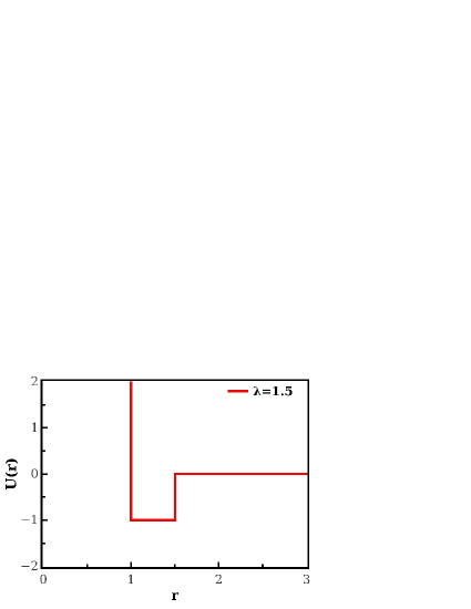
Figure 1: Schematic representation of the SW pair potential of range $\lambda=1.5$. In the framework of the CFA the potential is approximated with $\alpha_{o}=\alpha_{1}=1000$, $\epsilon_{1}=0$ and $\epsilon_{2}=-1$, respectively.

The studied system is composed by $N=1372$ spherical particles, initially distributed on a FCC configuration with random velocities that satisfy the equipartition theorem Allen1991 . We use standard reduced units of length, temperature and time defined as $r^{*}\equiv r/\sigma$, $T^{*}=k_{B}T/\epsilon$ and $t^{*}=t/\tau$, respectively. Where, $\sigma,m,\epsilon$ and $\tau=\sqrt{m\sigma^{2}/\epsilon}$ are the usual units of length, mass, energy and time, respectively. In the same line, the packing fraction is defined as $\eta=N\pi\sigma^{3}/6V$, with $V$ the simulation box volume. Thus, the reduced density is given by $\rho^{*}=6\eta/\pi$.

The equations of motion are integrated with the velocity Verlet algorithm Swope1982 employing a time step $\Delta t=1\times 10^{-5}\tau$ to guarantee the numerical stability of the CFA. It is worth to point out that in difference with previous works Orea2013 ; Padilla2017 ,SecIV we do not use an external input table to compute any the interaction potential or the force between the fluid particles, instead such contributions are explicitly computed at each time step in order to avoid numerical inaccuracies. In all cases, we performed $1.1\times 10^{9}$ integration steps, where $1\times 10^{8}$ integration steps were carried out to reach thermal equilibrium and the subsequent time steps were used to compute the static and dynamic properties like the radial distribution function and the mean-squared displacement, respectively. The statical uncertainties associated with the time correlation function are obtained according to the procedure describe in Ref. Swope1982 . The system temperature is kept fixed by a simple velocity scaling as the thermostat Frenkel .

IV Self-diffusion coefficient of the square-well fluid.

IV.1 Mean-square displacement

As was mentioned in Sec. II, in order to determine the self-diffusion coefficient by means of the Eq. (8), the knowledge of the MSD is needed, which is computed directly from the MD simulations. The behavior of MSD for several values of $\lambda$ at the reduced temperature $T^{*}=1.5$ and the packing fraction $\eta=0.3$ is shown in Fig. 2.

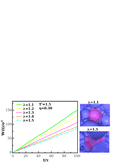
Figure 2: Mean square displacement for SW fluid particles at several values of the range interaction potential $\lambda=1.1,1.2,1.3,1.4,1.5$. In all cases the fluid is at the temperature $T^{*}=1.5$ and packing fraction $\eta=0.30$. The snapshot presented correspond to range interaction (top) $\lambda=1.1$ and (bottom) $\lambda=1.5$, respectively, at the thermodynamic conditions mentioned.

As one can see in Fig. 2, the magnitude of the MSD decreases as the attraction range of the SW potential increases, those differences are magnified at low values of $\lambda$. Since the MSD can be understood as the measure of one particle position deviation with respect to a reference position over time, in this scenario, the decrease of the MSD implies that fluid particles are more localized. This behavior is due to an increment of $\lambda$, or equivalent, given any particle, an increment of the surrounding fluid particles. This observation can be corroborated with the snapshots in Fig. 2, where we have selected a random particle, which is surrounding by an attractive spherical (red) shell of diameter $\lambda\sigma$. As can be seen in the snapshots of this figure, as the $\lambda\sigma$ value increase the number of neighbor particles also does for a system at the same thermodynamic state. Of course, for a fixed values of $\lambda\sigma$ and $T^{*}$ the MSD has also a magnitude decrement as the packing fraction (density) increases.

IV.2 Self-Diffusion coefficient

From the long time behavior of the MSD we extract the value of $D$ as a function of the packing fraction for different values of $\lambda$, see Fig. 3. Our mathematical approach to determine $D$ lead us an estimation of it with a high degree of numerical accuracy, that gives us, for all cases, error bars much more smaller than the symbol size.

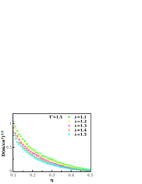
Figure 3: Self-diffusion coefficient $D$ for SW fluids as a function of the packing fraction at different values of the interaction potential range $\lambda=1.1,1.2,1.3,1.4,1.5$. In all cases, the reduced temperature is $T^{*}=1.5$.

As one could expect, $D$ decreases as the packing fraction of the fluid increases independently of the potential interaction range. However and surprisingly, in general, the magnitude of $D$ is greater for low values of $\lambda$ if one sees at the same value of the packing fraction. These differences decreases as the attractive interaction range increases and as it is expected such differences are lost at the high concentration regime where the fluid is dynamical arrested. The first fluid that experiences the arrest is the one with the greater attraction range of this study, $\lambda=1.5$, and it happens, approximately, at $\eta\approx 0.49$.

For the self-diffusion coefficient, as can one can see in Fig. 3, the interaction potential parameters of the SW fluid, $\lambda$ and $\epsilon$, are highly relevant at low and intermediate packing fractions, i.e., for $\eta<0.3$. In the high concentration regime the hard-core interaction between particles dominates and the dynamical behavior tends to be similar, independently from the potential interaction range.

IV.3 Test of the Enskog method for SW fluids

In Section II, we summarized the expressions needed to compute $D$ in the framework of the Enskog theory. Although, from theoretical point of view, there are several approaches to compute $D$, the Eq. (1) is the first proposal given in terms of the Enskog theory, but, as has been demonstrated previously XinYu2001 , this expression it is not suitable to predict $D$ at moderate and high concentrations. In fact, as one can see in Fig. 4, the Eq. (1) totally fails at moderate concentration, i.e., $\eta>0.2$, and low values of $\lambda\sigma$, whereas as the attractive range interaction is increased an oscillatory behavior can be glimpsed at moderate concentrations. On the other hand, the predictions of Eq. (4) for $D$ overcomes the issues aforementioned despite of at low concentrations predicts greater values of $D$ than the Eq. (1).

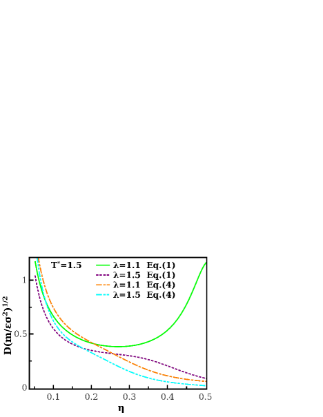
Figure 4: Comparison between the self-diffusion coefficient, $D$, predicted with Eqs. (1) and (4) obtained with the Enskog method as a function of the packing fraction.

Notwithstanding there exists different functional forms to predict $D$ for the SW fluid, it is a matter of fact that the agreement between them is questioned. In this line of thoughts, the success of some particular approach depends on the assumptions done to its deduction. In this way, computer simulations are used to test such theoretical proposals, nevertheless, and despite of the plethora of results about SW fluid, its dynamical properties are far less studied. In Fig. 5, we have shown a systematically study of self-diffusion coefficient and our computer simulation results are compared with those provided by Eq. (4).

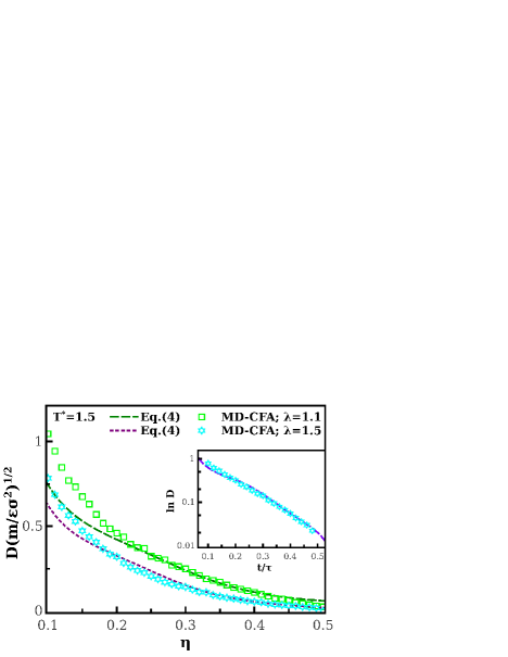
Figure 5: Comparison between the self-diffusion coefficient, $D$, predicted with (lines) the Enskog method Eq. (4) and results from (dots) MD within the CFA approach as a function of the packing fraction for the limit cases of our study $\lambda=1.1$ and $\lambda=1.5$ for the reduced temperature $T^{*}=1.5$.

In Fig. 5, we compare the lowest and highest values of $\lambda$ used in this work. We found a well qualitative agreement between the simulation results and the predictions given by Eq. (4), see the inset of Fig. 5. However, a closer inspection revels us differences between both results at low concentrations that are bigger than the acceptable tolerance. The Eq. (4) given by Yu XinYu2001 uses simulation results of the SW fluid at moderate and high concentrations to proposed the correction functions $f_{R}\left(\rho^{*}\right)$ and $f_{S}\left(\rho^{*}\right)$, given by Eqs. (5) and (6), respectively. For that, one could not expect a good performance of this approach at low packing fraction. Thus, our simulation results can be used to calibrate theoretical approaches in order to properly describe the low concentration regime, however, for the time being, such analysis it is out of the scope of this contribution.

V Concluding remarks

In this paper, we have performed a systematically study of the self-diffusion coefficient, $D$, of the SW fluid by means of molecular dynamics simulations within the constant force approach in the canonical $(N,V,T)$ ensemble. From the analysis of the simulation data, we show that, for a fixed temperature and low density, the magnitude of $D$ is higher for low values of the attractive interaction range than for the higher values of $\lambda$, at the same thermodynamic states. The increment of the attractive range in the potential causes a higher localization of the fluid particles (see the snapshots in Fig. 2), leading to a decrease of $D$ independently of the packing fraction. On the other hand, our results exhibits a very well agreement with the theoretical predictions of the Enskog method corrected by Yu XinYu2001 at moderated and high packing fractions, however, at low densities such agreement is lost.

Furthermore, we have provided new simulation data results for $D$ in a wide range of densities and different values of the attractive range interaction not reported previously. Thus, this results can be used to improve the correction functions in the theoretical descriptions, or to provide new and more sophisticated empirical relations. As well, the CFA manifest itself as a valuable tool, not only to determine the statistical properties of non-continuous potential but also its dynamical behavior. Finally, the mathematical framework reported in this work can be employed for both the determination of structural and dynamical properties of liquids or even colloidal systems that are characterized with the SW potential Valadez2012 ; Zhao2017 .

- (1) J. A. Barker and D. Henderson, “Perturbation theory and equation of state for fluids: The square well potential,” J. Chem. Phys., vol. 47, no. 8, pp. 2856–2861, 1967.
- (2) W. R. Smith, D. Henderson, and J. A. Barker, “Approximate evaluation of the second‐order term in the perturbation theory of fluids,” J. Chem. Phys., vol. 53, pp. 508–515, 1970.
- (3) W. R. Smith, D. Henderson, and J. A. Barker, “Perturbation theory and the radial distribution function of the squarewell fluid,” J. Chem. Phys., vol. 55, no. 8, pp. 4027–4033, 1971.
- (4) D. Henderson, J. A. Barker, and W. R. Smith, “Calculation of the contact value of the first‐ and second‐order terms in the perturbation expansion of the radial distribution function for the square‐well potential,” J. Chem. Phys., vol. 64, no. 10, pp. 4244–4245, 1976.
- (5) D. Henderson, O. H. Scalise, and W. R. Smith, “Monte carlo calculations of the equation of state of the square well fluid as a function of well width,” J. Chem. Phys., vol. 72, no. 4, pp. 2431–2438, 1980.
- (6) D. D. Carley, “Equations of state for a square well gas from a parametric integral equation,” J. Chem. Phys., vol. 67, no. 3, pp. 1267–1272, 1977.
- (7) D. D. Carley and A. C. Dotson, “Integral equation and perturbation method of calculating thermodynamic functions for a square-well fluid,” Phys. Rev. A, vol. 23, no. 3, pp. 1411–1418, 1981.
- (8) D. D. Carley, “Thermodynamic properties of a squarewell fluid in the liquid and vapor regions,” J. Chem. Phys., vol. 78, no. 9, pp. 5776–5781, 1983.
- (9) A. de Lonngi and F. de1 Rio, “Square well perturbation theory of fluids,” Mol. Phys., vol. 48, no. 2, pp. 293–313, 1983.
- (10) A. de Lonngi and F. de1 Rio, “Square-well perturbation theory for the structure of simple fluids,” Mol. Phys., vol. 56, no. 3, pp. 691–700, 1985.
- (11) F. de1 Rio and L. Lira, “Properties of the square-well fluid of variable width i. short-range expansion,” Mol. Phys., vol. 61, no. 2, pp. 275–292, 1987.
- (12) F. de1 Rio and L. Lira, “Properties of the square‐well fluid of variable width. ii. the mean field term,” J. Chem. Phys., vol. 87, no. 12, pp. 7179–7183, 1987.
- (13) A. L. Benavides and F. de1 Rio, “Properties of the square-well fluid of variable width iii. long-range expansion,” Mol. Phys., vol. 68, no. 5, pp. 983–1000, 1989.
- (14) A. L. Benavides, J. Alejandre, and F. de1 Rio, “Properties of the square-well fluid of variable width: Iv. molecular dynamics test of the van der waals and long-range approximations,” Mol. Phys., vol. 74, no. 2, pp. 321–331, 1991.
- (15) A. Gil-Villegas, F. de1 Rio, and A. L. Benavides, “Deviations from corresponding-states behavior in the vapor-liquid equilibrium of the square-well fluid,” Fluid Phase Equilibria, vol. 119, no. 2, pp. 97–112, 1996.
- (16) Rotenberg, “Monte carlo equation of state for hard spheres in an attractive square well,” J. Chem. Phys., vol. 43, no. 4, pp. 1198–1201, 1965.
- (17) F. Lado and W. W. Wood, “N dependence in monte carlo studies of the square‐well system,” J. Chem. Phys., vol. 49, no. 9, pp. 4244–4245, 1968.
- (18) Y. Rosenfeld and R. Thieberger, “Monte carlo and perturbation calculations for the square well fluid: Dependence on the square well range,” J. Chem. Phys., vol. 63, no. 5, pp. 1875–1877, 1975.
- (19) K. D. Scarfe, I. L. McLaughlin, and A. F. Collings, “The transport coefficients for a fluid of square‐well rough spheres: Comparison with methane,” Mol. Phys., vol. 65, no. 8, pp. 2991–2994, 1976.
- (20) L. Vega, E. de Miguel, L. F. Rull, G. Jackson, and I. A. McLure, “Phase equilibria and critical behavior of squarewell fluids of variable width by gibbs ensemble monte carlo simulation,” J. Chem. Phys., vol. 96, no. 3, pp. 2296–2305, 1992.
- (21) E. Schöll-Paschinger, A. L. Benavides, and R. Castañeda-Priego, “Vapor-liquid equilibrium and critical behavior of the square-well fluid of variable range: A theoretical study,” J. Chem. Phys., vol. 123, no. 23, pp. 234513–1–234513–9, 2005.
- (22) A. Gil-Villegas, A. Galindo, P. J. Whitehead, S. J. Mills, G. Jackson , and A. N. Burgess, “Statistical associating fluid theory for chain molecules with attractive potentials of variable range,” J. Chem. Phys., vol. 106, no. 10, pp. 4168–4186, 1997.
- (23) Y. Duda, “Square-well fluid modelling of protein liquid-vapor coexistence,” J. Chem. Phys., vol. 130, no. 11, pp. 116101–1–116101–2, 2009.
- (24) C. McCabe and G. Jackson, “Saft-vr modelling of the phase equilibrium of long-chain n-alkanes,” Phys. Chem. Chem. Phys., vol. 1, no. 9, pp. 2057–2064, 1999.
- (25) C. McCabe and A. Galindo, SAFT Associating Fluids and Fluid Mixtures. In Applied Thermodynamics of Fluids. Goodwin, A. R. H., Sengers, J. V., Peters, C. J., Eds.; Royal Society of Chemistry: London, 2010.
- (26) J. Millat, J. H. Dymond, and C. A. Nieto de Castro, Transport properties of fluids: Their correlation, prediction and estimation. Cambridge University Press, 1996.
- (27) M. P. Allen and D. J. Tildesley, Computer Simulation of Liquids. Claredon Press, 1991.
- (28) B. J. Alder and T. E. Wainwright, “Studies in molecular dynamics. i. general method,” J. Chem. Phys., vol. 31, no. 2, pp. 459–466, 1959.
- (29) W. P. Krekelberg, J. Mittal, V. Ganesan, and T. M. Trukett, “How short-range attractions impact the structural order, self-diffusivity, and viscosity of a fluid,” J. Chem. Phys., vol. 127, pp. 044502–1–044502–8, 2007.
- (30) D. K. Dysthe, A. H. Fuchs, and M. Durandeau, “Fluid transport properties by equilibrium molecular dynamics. ii. multicomponent systems,” J. Chem. Phys., vol. 110, no. 8, pp. 4060–4067, 1999.
- (31) K. Meler, A. Laesecke, and S. Kebelac, “Transport coefficients of the lennard-jones model fluid. i. viscosity,” J. Chem. Phys., vol. 121, no. 8, pp. 3671–3687, 2004.
- (32) K. Meler, A. Laesecke, and S. Kebelac, “Transport coefficients of the lennard-jones model fluid. ii self-diffusion,” J. Chem. Phys., vol. 121, no. 19, pp. 9526–9535, 2004.
- (33) D. Frenkel and B. Smit, Understanding Molecular Simulation. Academic Press, 2002.
- (34) P. Orea and G. Odriozola, “Constant-force approach to discontinuous potentials,” J. Chem. Phys., vol. 138, pp. 214105–1–214105–4, 2013.
- (35) L. A. Padilla and A. L. Benavides, “The constant force continuous molecular dynamics for potentials with multiple discontinuities,” J. Chem. Phys., vol. 147, pp. 034502–1–034502–6, 2017.
- (36) Y. Reyes, M. Bárcenas, G. Odriozola, and P. Orea, “Thermodynamic properties of triangle-well fluids in two dimensions: Mc and md simulations,” J. Chem. Phys., vol. 145, pp. 174505–1–174505–4, 2016.
- (37) J. H. Dymond, “Hard-sphere theories of transport properties,” Chem. Soc. Rev., vol. 14, pp. 317–356, 1985.
- (38) R. J. Speedy, “Diffusion in the hard sphere fluid,” Mol. Phys., vol. 62, no. 2, pp. 509–515, 1987.
- (39) H. C. Longuet-Higgins and J. P. Valleau, “Transport coefficients of dense fluids of molecules interacting according to a square well potential,” Mol. Phys., vol. 1, no. 3, pp. 284–294, 1958.
- (40) H. T. Davis, S. A. Rice, and J. V. Sengers, “On the kinetic theory of dense fluids. ix. the fluid of rigid spheres with a square‐well attraction,” J. Chem. Phys., vol. 35, no. 6, pp. 2210–2233, 1961.
- (41) I. A. McLaughlin and H. T. Davis, “Kinetic theory of dense fluid mixtures. i. square‐well model,” J. Chem. Phys., vol. 45, no. 6, pp. 2020–2031, 1966.
- (42) R. Brown and H. T. Davis, “Kinetic theory of dense fluid mixtures. i. square‐well model,” J. Phys. Chem., vol. 75, no. 13, pp. 1970–1974, 1971.
- (43) Yang-Xing Yu, Ming-Han Han, and Guang-Hua Gao, “Self-diffusion in a fluid of square-well spheres,” Phys. Chem. Chem. Phys., vol. 3, pp. 437–443, 2001.
- (44) J. Chang and S. I. Sandler, “A real function representation for the structure of the hard-sphere fluid,” Mol. Phys., vol. 81, no. 3, pp. 735–744, 1994.
- (45) J. Chang and S. I. Sandler, “A completely analytic perturbation theory for the square-well fluid of variable well width,” Mol. Phys., vol. 81, no. 3, pp. 745–744, 1994.
- (46) J. A. Barker and D. Henderson, “Monte carlo values for the radial distribution function of a system of fluid hard spheres,” Mol. Phys., vol. 21, no. 1, pp. 187–191, 1971.
- (47) J. W. Duffy, K. C. Mo, and K. E. Gubbins, “Models for self‐diffusion in the square well fluid,” J. Chem. Phys., vol. 94, no. 4, pp. 3132–3140, 1991.
- (48) W. E. Alley and B. J. Alder, “Studies in molecular dynamics. xv. high temperature description of the transport coefficients,” J. Chem. Phys., vol. 63, no. 9, pp. 3764–3768, 1975.
- (49) J.P. J. Michels and N. J. Trappeniers, “Molecular dynamical calculations of the transport properties of a square-well fluid: V. the coefficient of self-diffusion,” Phys. A, vol. 116, pp. 516–525, 1982.
- (50) J.P. J. Michels and N. J. Trappeniers, “Molecular dynamical calculations of the transport properties of a square-well fluid: V. the coefficient of self-diffusion,” Chem. Phys. Lett., vol. 33, no. 2, pp. 195–200, 1975.
- (51) H. Liua, C. M. Silva, and E. A. Macedo, “Unified approach to the self-diffusion coefficients of dense fluids over wide ranges of temperature and pressure—hard-sphere, square-well, lennard–jones and real substances,” Chem. Eng. Sci., vol. 53, no. 13, pp. 2403–2422, 1998.
- (52) R. Zwanzig, “Time-correlation functions and transport coefficients in statistical mechanics,” Annu. Rev. Phys. Chem., vol. 16, pp. 67–102, 1965.
- (53) W. C. Swope, H. C. Andersen, P. H. Berens, and K. R. Wilson, “A computer simulation method for the calculation of equilibrium constants for the formation of physical clusters of molecules: Application to small water clusters,” J. Chem. Phys., vol. 76, no. 1, pp. 637–649, 1982.
- (54) N. E. Valadez-Pérez, A. L. Benavídes, E. Schöll-Paschinger, and R. Castañeda-Priego, “Phase behavior of colloids and proteins in aqueous suspensions: Theory and computer simulations,” J. Chem. Phys., vol. 137, no. 8, pp. 084905–1–084905–15, 2012.
- (55) B. Zhao, T. Lindeboom, S. Benner, G. Jackson, A. Galindo, and C. K. Hall, “Predicting the fluid-phase behavior of aqueous solutions of elp (vpgvg) sequences using saft-vr,” Langmuir, vol. 33, no. 42, pp. 11733–11745, 2017.