MIMO-OTFS in High-Doppler Fading Channels: Signal Detection and Channel Estimation

Abstract

Orthogonal time frequency space (OTFS) modulation is a recently introduced multiplexing technique designed in the 2-dimensional (2D) delay-Doppler domain suited for high-Doppler fading channels. OTFS converts a doubly-dispersive channel into an almost non-fading channel in the delay-Doppler domain through a series of 2D transformations. In this paper, we focus on MIMO-OTFS which brings in the high spectral and energy efficiency benefits of MIMO and the robustness of OTFS in high-Doppler fading channels. The OTFS channel-symbol coupling and the sparse delay-Doppler channel impulse response enable efficient MIMO channel estimation in high Doppler environments. We present an iterative algorithm for signal detection based on message passing and a channel estimation scheme in the delay-Doppler domain suited for MIMO-OTFS. The proposed channel estimation scheme uses impulses in the delay-Doppler domain as pilots for estimation. We also compare the performance of MIMO-OTFS with that of MIMO-OFDM under high Doppler scenarios.

keywords: OTFS modulation, MIMO-OTFS, 2D modulation, delay-Doppler domain, MIMO-OTFS signal detection, channel estimation.

I Introduction

Future wireless systems including 5G systems need to operate in dynamic channel conditions, where operation in high mobility scenarios (e.g., high-speed trains) and millimeter wave (mm Wave) bands are envisioned. The wireless channels in such scenarios are doubly-dispersive, where multipath propagation effects cause time dispersion and Doppler shifts cause frequency dispersion [1]. OFDM systems are usually employed to mitigate the effect of inter-symbol interference (ISI) caused by time dispersion [2]. However, Doppler shifts result in inter-carrier interference (ICI) in OFDM and degrades performance [3]. An approach to jointly combat ISI and ICI is to use pulse shaped OFDM systems [4]-[6]. Pulse shaped OFDM systems use general time-frequency lattices and optimized pulse shapes in the time-frequency domain. However, systems that employ the pulse shaping approach do not efficiently address the need to support high Doppler shifts.

Orthogonal time frequency space (OTFS) modulation is a recently proposed multiplexing scheme [7]-[10] which meets the high-Doppler signaling need through a different approach, namely, multiplexing the modulation symbols in the delay-Doppler domain (instead of multiplexing symbols in time-frequency domain as in traditional modulation techniques such as OFDM). OTFS waveform has been shown to be resilient to delay-Doppler shifts in the wireless channel. For example, OTFS has been shown to achieve significantly better error performance compared to OFDM for vehicle speeds ranging from 30 km/h to 500 km/h in 4 GHz band, and that the robustness to high-Doppler channels (e.g., 500 km/h vehicle speeds) is especially notable, as OFDM performance breaks down in such high-Doppler scenarios [9]. When OTFS waveform is viewed in the delay-Doppler domain, it corresponds to a 2D localized pulse. Modulation symbols, such as QAM symbols, are multiplexed using these pulses as basis functions. The idea is to transform the time-varying multipath channel into a 2D time-invariant channel in the delay-Doppler domain. This results in a simple and symmetric coupling between the channel and the modulation symbols, due to which significant performance gains compared to other multiplexing techniques are achieved [7]. OTFS modulation can be architected over any multicarrier modulation by adding pre-processing and post-processing blocks. This is very attractive from an implementation view-point.

Recognizing the promise of OTFS in future wireless systems, including mmWave communication systems [10], several works on OTFS have started emerging in the recent literature [11]-[16]. These works have addressed the formulation of input-output relation in vectorized form, equalization and detection, and channel estimation. Multiple-input multiple-output (MIMO) techniques along with OTFS (MIMO-OTFS) can achieve increased spectral/energy efficiencies and robustness in rapidly varying MIMO channels. It is shown in [7] that OTFS approaches channel capacity through linear scaling of spectral efficiency with the MIMO order. We, in this paper, consider the signal detection and channel estimation aspects in MIMO-OTFS.

Figure 1: OTFS modulation scheme.

Our contributions can be summarized as follows. We first present a vectorized input-output formulation for the MIMO-OTFS system. Initially, we assume perfect channel knowledge at the receiver and employ an iterative algorithm based on message passing for signal detection. The algorithm has low complexity and it achieves very good performance. For example, in a $2\times 2$ MIMO-OTFS system, a bit error rate (BER) of $10^{-5}$ is achieved at an SNR of about 14 dB for a Doppler of 1880 Hz (500 km/hr speed at 4 GHz). For the same system, MIMO-OFDM BER performance floors at a BER of 0.02. Next, we relax the perfect channel estimation assumption and present a channel estimation scheme in the delay-Doppler domain. The proposed scheme uses impulses in the delay-Doppler domain as pilots for MIMO-OTFS channel estimation. The proposed scheme is simple and effective in high-Doppler MIMO channels. For example, compared to the case of perfect channel knowledge, the proposed scheme loses performance only by less than a fraction of a dB.

The rest of the paper is organized as follows. The OTFS modulation is introduced in Sec. II. The MIMO-OTFS system model and the vectorized input-output relation are developed in Sec. III. MIMO-OTFS signal detection using message passing and the resulting BER performance are presented in Sec. IV. The channel estimation scheme in the delay-Doppler domain and the achieved performance are presented in Sec. V. Conclusions are presented in Sec. VI.

II OTFS Modulation

OTFS modulation uses the delay-Doppler domain for multiplexing the modulation symbols and for channel representation. When the channel impulse response is represented in the delay-Doppler domain, the received signal $y(t)$ is the sum of reflected copies of the transmitted signal $x(t)$, which are delayed in time ($\tau$), shifted in frequency ($\nu$), and multiplied by the complex gain $h(\tau,\nu)$ [8]. Thus, the coupling between an input signal and the channel in this domain is given by the following double integral:

$$y(t)=\int_{\nu}\int_{\tau}h(\tau,\nu)x(t-\tau)e^{j2\pi\nu(t-\tau)}\mathrm{d}\tau\mathrm{d}\nu.$$ (1)

The block diagram of the OTFS modulation scheme is shown in Fig. 1. The inner box is the familiar time-frequency multicarrier modulation, and the outer box with a pre- and post-processor implements the OTFS modulation scheme in the delay-Doppler domain. The information symbols $x[k,l]$ (e.g., QAM symbols) residing in the delay-Doppler domain are first transformed to the familiar time-frequency (TF) domain signal $X[n,m]$ through the 2D inverse symplectic finite Fourier transform (ISFFT) and windowing. The Heisenberg transform is then applied to the TF signal $X[n,m]$ to transform to the time domain signal $x(t)$ for transmission. At the receiver, the received signal $y(t)$ is transformed back to a TF domain signal $Y[n,m]$ through Wigner transform (inverse Heisenberg transform). $Y[n,m]$ thus obtained is transformed to the delay-Doppler domain signal $y[k,l]$ through the symplectic finite Fourier transform (SFFT) for demodulation.

In the following subsections, we describe the signal models in TF modulation and OTFS modulation. Let $T$ denote the TF modulation symbol time and $\Delta f$ denote the subcarrier spacing. Let $x[k,l]$, $k=0,\cdots,N-1$, $l=0,\cdots,M-1$ be the information symbols transmitted in a given packet burst. Let $W_{tx}[n,m]$ and $W_{rx}[n,m]$ denote the transmit and receive windows, respectively.

II-A Time-frequency modulation

• Let $\varphi_{tx}(t)$ and $\varphi_{rx}(t)$ denote the transmit and receive pulses, respectively, which are bi-orthogonal with respect to time and frequency translations. Signal in the TF domain $X[n,m]$, $n=0,\cdots,N-1$, $m=0,\cdots,M-1$ is transmitted in a given packet burst.

• TF modulation/Heisenberg transform: The signal in the time-frequency domain $X[n,m]$ is transformed to the time domain signal $x(t)$ using the Heisenberg transform given by

  $$x(t)=\sum_{n=0}^{N-1}\sum_{m=0}^{M-1}X[n,m]\varphi_{tx}(t-nT)e^{j2\pi m\Delta f(t-nT)}.$$ (2)

• TF demodulation/Wigner transform: At the receiver, the time domain signal is transformed back to the TF domain using Wigner transform given by

  $$Y[n,m]=A_{\varphi_{rx},y}(\tau,\nu)|_{\tau=nT,\nu=m\Delta f},$$ (3)

  where $A_{\varphi_{rx},y}(\tau,\nu)$ is the cross ambiguity function given by

  $$A_{\varphi_{rx},y}(\tau,\nu)=\int\varphi_{rx}^{*}(t-\tau)y(t)e^{-j2\pi\nu(t-\tau)}\mathrm{d}t,$$ (4)

and $y(t)$ is related to $x(t)$ by (1). The relation between $Y[n,m]$ and $X[n,m]$ for TF modulation can be derived as [9]

$$Y[n,m]=H[n,m]X[n,m]+V[n,m],$$ (5)

where $V[n,m]$ is the additive white Gaussian noise and $H[n,m]$ is given by

$$H[n,m]=\int_{\tau}\int_{\nu}h(\tau,\nu)e^{j2\pi\nu nT}e^{-j2\pi(\nu+m\Delta f)\tau}\mathrm{d}\nu\mathrm{d}\tau.$$ (6)

II-B OTFS modulation

• Let $X_{p}[n,m]$ be the periodized version of $X[n,m]$ with period $(N,M)$. The SFFT of $X_{p}[n,m]$ is given by

  $$x_{p}[k,l]=\sum_{n=0}^{N-1}\sum_{m=0}^{M-1}X_{p}[n,m]e^{-j2\pi({nk\over N}-{ml\over M})},$$ (7)

  and the ISFFT is $X_{p}[n,m]=SFFT^{-1}(x[k,l])$, given by

  $$X_{p}[n,m]={1\over MN}\sum_{k=0}^{N-1}\sum_{l=0}^{M-1}x[k,l]e^{j2\pi({nk\over N}-{ml\over M})}.$$ (8)

• Information symbols $x[k,l]$, $k=0,\cdots,N-1$, $l=0,\cdots,M-1$, are transmitted in a given packet burst.

• OTFS transform/pre-processing: The information symbols in the delay-Doppler domain $x[k,l]$ are mapped to TF domain symbols $X[n,m]$ as

  $$X[n,m]=W_{tx}[n,m]SFFT^{-1}(x[k,l]),$$ (9)

  where $W_{tx}[n,m]$ is the transmit windowing square summable function.

• $X[n,m]$ thus obtained is in the TF domain and it is TF modulated as described in the previous subsection, and $Y[n,m]$ is obtained by (3).

• OTFS demodulation/post-processing: A receive window $W_{rx}[n,m]$ is applied to $Y[n,m]$ and periodized to obtain $Y_{p}[n,m]$ which has the period $(N,M)$, as

  $$Y_{W}[n,m] = W_{rx}[n,m]Y[n,m],$$

  $$Y_{p}[n,m] = \sum_{k,l=-\infty}^{\infty}Y_{W}[n-kN,m-lM].$$ (10)

  The symplectic finite Fourier transform is then applied to $Y_{p}[n,m]$ to convert it from TF domain back to delay-Doppler domain $\hat{x}[k,l]$, as

  $$\hat{x}[k,l]=SFFT(Y_{p}[n,m]).$$ (11)

The input-output relation in OTFS modulation can be derived as [9]

$$\hat{x}[k,l]={1\over MN}\sum_{m=0}^{M-1}\sum_{n=0}^{N-1}x[n,m]h_{w}\left({k-n\over NT},{l-m\over M\Delta f}\right)+v[k,l],$$ (12)

where

$$h_{w}\left({k-n\over NT},{l-m\over M\Delta f}\right)=h_{w}(\nu^{\prime},\tau^{\prime})|_{\nu^{\prime}={k-n\over NT},\tau^{\prime}={l-m\over M\Delta f}},$$ (13)

where $h_{w}(\nu^{\prime},\tau^{\prime})$ is the circular convolution of the channel response with a windowing function $w(\tau,\nu)$, given by

$$h_{w}(\nu^{\prime},\tau^{\prime})=\int_{\nu}\int_{\tau}h(\tau,\nu)w(\nu^{\prime}-\nu,\tau^{\prime}-\tau)\mathrm{d}\tau\mathrm{d}\nu,$$ (14)

where $w(\tau,\nu)$ is given by

$$w(\tau,\nu)=\sum_{m=0}^{M-1}\sum_{n=0}^{N-1}W_{tx}[n,m]W_{rx}[n,m]e^{-j2\pi(\nu nT-\tau m\Delta f)}.$$ (15)

Figure 2: MIMO-OTFS modulation scheme.

II-C Vectorized formulation of the input-output relation

Consider a channel with $P$ signal propagation paths (taps). Let the path $i$ be associated with a delay $\tau_{i}$, a Doppler $\nu_{i}$, and a fade coefficient $h_{i}$. The channel impulse response in the delay-Doppler domain can be written as

$$h(\tau,\nu)=\sum_{i=1}^{P}h_{i}\delta(\tau-\tau_{i})\delta(\nu-\nu_{i}).$$ (16)

Assume that the windows used in modulation, $W_{tx}[n,m]$ and $W_{rx}[n,m]$ are rectangular. Define $\tau_{i}={\alpha_{i}\over M\Delta f}$ and $\nu_{i}={\beta_{i}\over NT}$, where $\alpha_{i}$ and $\beta_{i}$ are integers denoting the indices of the delay tap (with delay $\tau_{i}$) and Doppler tap (with Doppler value $\nu_{i}$). In practice, although the delay and Doppler values are not exactly integer multiples of the taps, they can be well approximated by a few delay-Doppler taps in the discrete domain [19]. With the above assumptions, the input-output relation for the channel in (16) can be derived as [12]

$$y[k,l]=\sum_{i=1}^{P}h_{i}^{\prime}x[((k-\beta_{i}))_{N},((l-\alpha_{i}))_{M})]+v[k,l].$$ (17)

where $h_{i}^{\prime}=h_{i}e^{-j2\pi\nu_{i}\tau_{i}}$. The above equation can be represented in vectorized form as [12]

$$\mathbf{y}=\mathbf{Hx}+\mathbf{v},$$ (18)

where $\mathbf{x},\mathbf{y},\mathbf{v}\in\mathbb{C}^{NM\times 1}$, $\mathbf{H}\in\mathbb{C}^{NM\times NM}$, the $(k+Nl)$th element of $\mathbf{x}$, $x_{k+Nl}=x[k,l]$, $k=0,\cdots,N-1,l=0,\cdots,M-1$, and the same relation holds for $\mathbf{y}$ and $\mathbf{z}$ as well. In this representation, there are only $P$ non-zero elements in each row and column of the equivalent channel matrix ($\mathbf{H}$) due to modulo operations.

III MIMO-OTFS Modulation

Consider a MIMO-OTFS system as shown in Fig. 2 with equal number of transmit ($n_{t}$) and receive antennas ($n_{r}$), i.e., $n_{t}=n_{r}=n_{a}$. Each antenna transmits OTFS modulated information symbols independently. Let the windows $W_{tx}[n,m]$, $W_{rx}[n,m]$ used for modulation be rectangular. Assume that the channel corresponding to $p$th transmit antenna and $q$th receive antenna has $P$ taps as in (16). Therefore, the channel representation can be written as

$$h_{qp}(\tau,\nu)=\sum_{i=1}^{P}h_{qp_{i}}\delta(\tau-\tau_{i})\delta(\nu-\nu_{i}),$$ (19)

$p=1,2,\cdots,n_{a}$, $q=1,2,\cdots,n_{a}$. Thus, we can use the vectorized formulation in Sec. II-C for each transmit and receive antenna pair to describe the input-output relation.

III-A Vectorized formulation of the input-output relation for MIMO-OTFS

Let $\mathbf{H}_{qp}$ denote the equivalent channel matrix corresponding to $p$th transmit antenna and $q$th receive antenna. Let $\mathbf{x}_{p}$ denote the $NM\times 1$ transmit vector from the $p$th transmit antenna and $\mathbf{y}_{q}$ denote the $NM\times 1$ received vector corresponding to $q$th receive antenna in a given frame. Then, similar to the system model in (18) for a SISO-OTFS, we can derive a linear system model describing the input and output for the MIMO-OTFS system as given below

$$\mathbf{y}_{1} = \mathbf{H}_{11}\mathbf{x}_{1}+\mathbf{H}_{12}\mathbf{x}_{2}+\cdots+\mathbf{H}_{1{n_{a}}}\mathbf{x}_{n_{a}}+\mathbf{v}_{1},$$

$$\mathbf{y}_{2} = \mathbf{H}_{21}\mathbf{x}_{1}+\mathbf{H}_{22}\mathbf{x}_{2}+\cdots+\mathbf{H}_{2{n_{a}}}\mathbf{x}_{n_{a}}+\mathbf{v}_{2},$$

$$\vdots$$

$$\mathbf{y}_{n_{a}} = \mathbf{H}_{{n_{a}}1}\mathbf{x}_{1}+\mathbf{H}_{{n_{a}}2}\mathbf{x}_{2}+\cdots+\mathbf{H}_{{n_{a}}{n_{a}}}\mathbf{x}_{n_{a}}+\mathbf{v}_{n_{a}}.\hskip 11.38109pt$$ (20)

Define

$$\ \mathbf{H}_{{\tiny\mbox{MIMO}}} =\begin{bmatrix}\mathbf{H}_{11}&\mathbf{H}_{12}&\dots&\mathbf{H}_{1{n_{a}}}\\ \mathbf{H}_{21}&\mathbf{H}_{22}&\dots&\mathbf{H}_{2{n_{a}}}\\ \vdots&\vdots&\ddots&\vdots\\ \mathbf{H}_{{n_{a}}1}&\mathbf{H}_{{n_{a}}2}&\dots&\mathbf{H}_{{n_{a}}{n_{a}}}\end{bmatrix},$$

$$\mathbf{x}_{{\tiny\mbox{MIMO}}}={[{\mathbf{x}_{1}}^{T},{\mathbf{x}_{2}}^{T},\cdots,{\mathbf{x}_{n_{a}}}^{T}]}^{T},\mathbf{y}_{{\tiny\mbox{MIMO}}}={[{\mathbf{y}_{1}}^{T},{\mathbf{y}_{2}}^{T},\cdots,{\mathbf{y}_{n_{a}}}^{T}]}^{T},$$

$$\mathbf{v}_{{\tiny\mbox{MIMO}}}={[{\mathbf{v}_{1}}^{T},{\mathbf{v}_{2}}^{T},\cdots,{\mathbf{v}_{n_{a}}}^{T}]}^{T}.$$

Then, (20) can be written as

$$\mathbf{y}_{{\tiny\mbox{MIMO}}}=\mathbf{H}_{{\tiny\mbox{MIMO}}}\mathbf{x}_{{\tiny\mbox{MIMO}}}+\mathbf{v}_{\tiny\mbox{MIMO}},$$ (21)

where $\mathbf{x}_{{\tiny\mbox{MIMO}}},\mathbf{y}_{{\tiny\mbox{MIMO}}},\mathbf{v}_{\tiny\mbox{MIMO}}\in\mathbb{C}^{{n_{a}}NM\times 1}$, $\mathbf{H}_{{\tiny\mbox{MIMO}}}\in\mathbb{C}^{{n_{a}}NM\times{n_{a}}NM}$. Thus, in this representation, each row and column of $\mathbf{H}_{{\tiny\mbox{MIMO}}}$ has only $n_{a}P$ non-zero elements due to modulo operations.

IV MIMO-OTFS Signal Detection

In this section, we present a MIMO-OTFS signal detection scheme using an iterative algorithm based on message passing and present a performance comparison between MIMO-OTFS and MIMO-OFDM in high-Doppler scenarios.

IV-A Algorithm for MIMO-OTFS signal detection

Let the sets of non-zero positions in the $b$th row and $a$th column of $\mathbf{H}_{{\tiny\mbox{MIMO}}}$ be denoted by $\zeta_{b}$ and $\zeta_{a}$, respectively. Using (21), the system can be modeled as a sparsely connected factor graph with ${n_{a}}NM$ variable nodes corresponding to the elements in $\mathbf{x}_{{\tiny\mbox{MIMO}}}$ and ${n_{a}}NM$ observation nodes corresponding to the elements in $\mathbf{y}_{{\tiny\mbox{MIMO}}}$. Each observation node $y_{b}$ is connected to the set of variable nodes {$x_{c},c\in\zeta_{b}$}, and each variable node $x_{a}$ is connected to the set of observation nodes {$y_{c},c\in\zeta_{a}$}. Also, $|\zeta_{b}|=|\zeta_{a}|={n_{a}}P$. The maximum a posteriori (MAP) decision rule for (21) is given by

$${\hat{\mathbf{x}}_{{\tiny\mbox{MIMO}}}}=\mathop{\text{argmax}}_{\mathbf{x}_{{\tiny\mbox{MIMO}}}\in\mathbb{A}^{n_{a}NM}}\mbox{Pr}(\mathbf{x}_{{\tiny\mbox{MIMO}}}|\mathbf{y}_{{\tiny\mbox{MIMO}}},\mathbf{H}_{{\tiny\mbox{MIMO}}}),$$ (22)

where $\mathbb{A}$ is the modulation alphabet (e.g., QAM) used. The detection as per (22) has exponential complexity. Hence, we use symbol by symbol MAP rule for $0\leq a\leq n_{a}NM-1$ for detection as follows:

$$\begin{split}\hat{x}_{a}&=\mathop{\text{argmax}}_{a_{j}\in\mathbb{A}}\mbox{Pr}(x_{a}=a_{j}|\mathbf{y}_{{\tiny\mbox{MIMO}}},\mathbf{H}_{{\tiny\mbox{MIMO}}})\\ &=\mathop{\text{argmax}}_{a_{j}\in\mathbb{A}}{1\over|\mathbb{A}|}\mbox{Pr}(\mathbf{y}_{{\tiny\mbox{MIMO}}}|x_{a}=a_{j},\mathbf{H}_{{\tiny\mbox{MIMO}}})\\ &\approx\mathop{\text{argmax}}_{a_{j}\in\mathbb{A}}\prod_{c\in\zeta_{a}}\mbox{Pr}(y_{c}|x_{a}=a_{j},\mathbf{H}_{{\tiny\mbox{MIMO}}}).\end{split}$$

The transmitted symbols are assumed to be equally likely and the components f $\mathbf{y}_{{\tiny\mbox{MIMO}}}$ are nearly independent for a given $x_{a}$ due to the sparsity in $\mathbf{H}_{{\tiny\mbox{MIMO}}}$. This can be solved using the message passing based algorithm described below. The message that is passed from the variable node $x_{a}$, for each $a=\{0,1,\cdots,n_{a}NM-1\}$, to the observation node $y_{b}$ for $b\in\zeta_{a}$, is the pmf denoted by $\textbf{p}_{ab}=\{p_{ab}(a_{j})|a_{j}\in\mathbb{A}\}$ of the symbols in the constellation $\mathbb{A}$. Let $H_{ab}$ denote the element in the $a$th row and $b$th column of $\mathbf{H}_{{\tiny\mbox{MIMO}}}$. The message passing algorithm is described as follows.

1:Inputs: $\mathbf{y}_{{\tiny\mbox{MIMO}}}$, $\mathbf{H}_{{\tiny\mbox{MIMO}}}$, $N_{iter}$: max. number of iterations.

2:Initialization: Iteration index $t=0$, pmf $\mathbf{p}_{ab}^{(0)}=1/|\mathbb{A}|\ \forall\ a\in\{0,1,\cdots,n_{a}NM-1\}$ and $b\in\zeta_{a}$.

3:Messages from $y_{b}$ to $x_{a}$: The mean $(\mu_{ba}^{(t)})$ and variance $((\sigma_{ba}^{(t)})^{2})$ of the interference term $I_{ba}$ are passed as messages from $y_{b}$ to $x_{a}$. $I_{ba}$ can be approximated as a Gaussian random variable and is given by

$$I_{ba}=\sum_{c\in\zeta_{b},c\neq a}x_{c}H_{b,c}+v_{b}.$$ (23)

The mean and variance of $I_{ba}$ are given by

$$\mu_{ba}^{(t)}=\mathbb{E}[I_{ba}]=\sum_{c\in\zeta_{b},c\neq a}\sum_{j=1}^{|\mathbb{A}|}p_{cb}^{(t)}(a_{j})a_{j}H_{b,c},$$

$$(\sigma_{ba}^{(t)})^{2}=\text{Var}[I_{ba}]$$

$$=\sum_{\begin{subarray}{c}c\in\zeta_{b}\\ c\neq a\end{subarray}}\Bigg{(}\sum_{j=1}^{\mathbb{|A|}}p_{cb}^{(t)}(a_{j})|a_{j}|^{2}|H_{b,c}|^{2}-\bigg{|}\sum_{j=1}^{\mathbb{|A|}}p_{cb}^{(t)}(a_{j})a_{j}H_{b,c}\bigg{|}^{2}\Bigg{)}$$

      $+\ \sigma^{2}.$

4:Messages from $x_{a}$ to $y_{b}$: Messages passed from variable nodes $x_{a}$ to observation nodes $y_{b}$ is the pmf vector $\textbf{p}_{ab}^{(t+1)}$ with the elements given by

$$p_{ab}^{(t+1)}=\Delta\ p_{ab}^{(t)}(a_{j})+(1-\Delta)\ p_{ab}^{(t-1)}(a_{j}),$$ (24)

where $\Delta\in(0,1]$ is the damping factor for improving convergence rate, and

$$p_{ab}^{(t)}\propto\prod_{c\in\zeta_{a},c\neq b}\text{Pr}(y_{c}|x_{a}=a_{j},\mathbf{H}_{{\tiny\mbox{MIMO}}}),$$ (25)

where

$$\text{Pr}(y_{c}|x_{a}=a_{j},\mathbf{H}_{{\tiny\mbox{MIMO}}})\propto\text{exp}\Bigg{(}{-|y_{c}-\mu_{ca}^{(t)}-H_{c,a}a_{j}|^{2}\over\sigma_{c,a}^{2(t)}}\Bigg{)}.$$

5:Stopping criterion: Repeat steps 3 & 4 till $\max\limits_{a,b,a_{j}}|p_{ab}^{(t+1)}(a_{j})-p_{ab}^{(t)}(a_{j})|<\epsilon$ (where $\epsilon$ is a small value) or the maximum number of iterations, $N_{iter}$, is reached.

6:Output: Output the detected symbol as

$$\hat{x}_{a}=\mathop{\text{argmax}}_{a_{j}\in\mathbb{A}}p_{a}(a_{j}),\>\>a\in{0,1,2,\cdots,n_{a}NM-1},$$ (26)

where

$$p_{a}(a_{j})=\prod_{c\in\zeta_{a}}\text{Pr}(y_{c}|x_{a}=a_{j},\mathbf{H}_{{\tiny\mbox{MIMO}}}).$$ (27)

IV-B Vectorized formulation of the input-output relation for MIMO-OFDM

In this subsection, in order to provide a performance comparison between MIMO-OTFS and MIMO-OFDM, we present the vectorized formulation of the input-output relation for MIMO-OFDM. OFDM uses the TF domain for signaling and channel representation. We will first derive the vectorized formulation for a SISO-OFDM and extend it to MIMO-OFDM. For a fair comparison with the OTFS modulation, we will consider $N$ consecutive OFDM blocks (each of size $M$) to be one frame, i.e., the transmit vector $\mathbf{x}_{{\tiny\mbox{OFDM}}}\in\mathbb{C}^{NM\times 1}$, and message passing detection is done jointly over one $NM\times 1$ frame. Consider the channel in (16). The time-delay representation $h(\tau,t)$ is related to the delay-Doppler representation $h(\tau,\nu)$ by a Fourier transform along the time axis, and is given by

$$h(\tau,t)=\sum_{i=1}^{P}h_{i}e^{j2\pi\nu_{i}t}\delta(\tau-\tau_{i}).$$ (28)

Sample the time axis at $t=nTs={n\over M\Delta f}$. The sampled time-delay representation $h(\tau,n)$ is given by

$$h(\tau,n)=\sum_{i=1}^{P}h_{i}e^{j2\pi\nu_{i}n\over M\Delta f}\delta(\tau-\tau_{i}).$$ (29)

Let $CP=P-1$ denote the cyclic prefix length used in each OFDM block and let $L=M+CP$. The size of one frame after cyclic prefix insertion to each block will then be $NL$. Let $\mathbf{T}_{CP}={[\mathbf{C}_{CP}^{T}\ \mathbf{I}_{M}]}^{T}$ denote the $L\times M$ matrix that inserts cyclic prefix for one block, where $\mathbf{C}_{CP}$ contains the last $CP$ rows of the identity matrix $\mathbf{I}_{M}$. Also, let $\mathbf{R}_{CP}=[{\bf 0}_{M\times CP}\ {\mathbf{I}}_{M}]$ denote the $M\times L$ the matrix that removes the cyclic prefix for one block [18]. Let $\mathbf{W}_{M\times M}$ and $\mathbf{W}^{H}_{M\times M}$ denote the DFT and IDFT matrices of size $M$. We use the following notations.

• $\mathbf{B}_{cpin}=\text{diag}\underbrace{(\mathbf{T}_{CP},\mathbf{T}_{CP},\cdots,\mathbf{T}_{CP})}_{N\ times}$ : cyclic prefix insertion matrix for $N$ consecutive OFDM blocks.

• $\mathbf{B}_{cpre}=\text{diag}\underbrace{(\mathbf{R}_{CP},\mathbf{R}_{CP},\cdots,\mathbf{R}_{CP})}_{N\ times}$ : cyclic prefix removal matrix for $N$ consecutive OFDM blocks.

• $\mathbf{D}=\text{diag}\underbrace{(\mathbf{W},\mathbf{W},\cdots,\mathbf{W})}_{N\ times}$ : DFT matrix for $N$ consecutive OFDM blocks.

• $\mathbf{D}^{H}=\text{diag}\underbrace{(\mathbf{W}^{H},\mathbf{W}^{H},\cdots,\mathbf{W}^{H})}_{N\ times}$ : IDFT matrix for $N$ consecutive OFDM blocks.

• The channel in the time-delay domain for a given frame can be written as a matrix $\mathbf{H}_{td}$ using (29) and has size $NL\times NL$.

Using the above, the end-to-end relationship in OFDM modulation can be described by the following linear model:

$$\mathbf{y}_{{\tiny\mbox{OFDM}}} =\underbrace{\mathbf{D}\mathbf{B}_{cpre}\mathbf{H}_{td}\mathbf{B}_{cpin}\mathbf{D}^{H}}_{\mathbf{H}_{{\tiny\mbox{OFDM}}}}\mathbf{x}_{{\tiny\mbox{OFDM}}}+\mathbf{v}$$

$$=\mathbf{H}_{{\tiny\mbox{OFDM}}}\mathbf{x}_{{\tiny\mbox{OFDM}}}+\mathbf{v},$$ (30)

where $\mathbf{x}_{{\tiny\mbox{OFDM}}},\mathbf{y}_{{\tiny\mbox{OFDM}}},\mathbf{v}\in\mathbb{C}^{NM\times 1}$, $\mathbf{H}_{{\tiny\mbox{OFDM}}}\in\mathbb{C}^{NM\times NM}$.

IV-B1 MIMO-OFDM

The vectorized formulation of the input-output relation for SISO-OFDM derived above can be extended to MIMO-OFDM in a similar fashion as was done for the MIMO-OTFS system described in Sec. III-A. Let $\mathbf{H}_{{{\tiny\mbox{OFDM}}}_{qp}}$ denote the equivalent channel matrix corresponding to $p$th transmit antenna and $q$th receive antenna. Let $\mathbf{x}_{{{\tiny\mbox{OFDM}}}_{p}}$ denote the $NM\times 1$ transmit vector from the $p$th transmit antenna and $\mathbf{y}_{{{\tiny\mbox{OFDM}}}_{q}}$ denote the $NM\times 1$ received vector corresponding to $q$th receive antenna in a given frame. Define

$$\ \mathbf{H}_{{\tiny\mbox{MIMO-OFDM}}} =\begin{bmatrix}\mathbf{H}_{{\tiny\mbox{OFDM}}_{11}}&\mathbf{H}_{{\tiny\mbox{OFDM}}_{12}}&\dots&\mathbf{H}_{{\tiny\mbox{OFDM}}_{1{n_{a}}}}\\ \mathbf{H}_{{\tiny\mbox{OFDM}}_{21}}&\mathbf{H}_{{\tiny\mbox{OFDM}}_{22}}&\dots&\mathbf{H}_{{\tiny\mbox{OFDM}}_{2n_{a}}}\\ \vdots&\vdots&\ddots&\vdots\\ \mathbf{H}_{{\tiny\mbox{OFDM}}_{n_{a}1}}&\mathbf{H}_{{\tiny\mbox{OFDM}}_{n_{a}2}}&\dots&\mathbf{H}_{{\tiny\mbox{OFDM}}_{n_{a}n_{a}}}\end{bmatrix},$$

$$\mathbf{x}_{{\tiny\mbox{MIMO-OFDM}}}={[{\mathbf{x}_{{\tiny\mbox{OFDM}}_{1}}}^{T},{\mathbf{x}_{{\tiny\mbox{OFDM}}_{2}}}^{T},\cdots,{\mathbf{x}_{{\tiny\mbox{OFDM}}_{n_{a}}}}^{T}]}^{T},$$

$$\mathbf{y}_{{\tiny\mbox{MIMO-OFDM}}}={[{\mathbf{y}_{{\tiny\mbox{OFDM}}_{1}}}^{T},{\mathbf{y}_{{\tiny\mbox{OFDM}}_{2}}}^{T},\cdots,{\mathbf{y}_{{\tiny\mbox{OFDM}}_{n_{a}}}}^{T}]}^{T}.$$

The input-output relation for MIMO-OFDM can be written as

$$\mathbf{y}_{{\tiny\mbox{MIMO-OFDM}}}=\mathbf{H}_{{\tiny\mbox{MIMO-OFDM}}}\mathbf{x}_{{\tiny\mbox{MIMO-OFDM}}}+\mathbf{v}_{\tiny\mbox{MIMO-OFDM}},$$ (31)

where $\mathbf{x}_{{\tiny\mbox{MIMO-OFDM}}},\mathbf{y}_{{\tiny\mbox{MIMO-OFDM}}},\mathbf{v}_{\tiny\mbox{MIMO-OFDM}}\in\mathbb{C}^{{n_{a}}NM\times 1}$ and $\mathbf{H}_{{\tiny\mbox{MIMO-OFDM}}}\in\mathbb{C}^{{n_{a}}NM\times{n_{a}}NM}$.

IV-C Performance results and discussions

In this subsection, we present the BER performance of MIMO-OTFS and compare it with that of MIMO-OFDM. Perfect channel knowledge is assumed at the receiver. Message passing algorithm is used for both MIMO-OTFS and MIMO-OFDM. A damping factor of 0.5 is used. The maximum number of iterations and the $\epsilon$ value used are 30 and 0.01, respectively. We use the channel model in (19) and the number of taps $P$ is taken to be 5. The delay-Doppler profile considered in the simulation is shown in Table I. Other simulation parameters used are given in Table II.

Path index $(i)$	$1$	$2$	$3$	$4$	$5$
Delay ($\tau_{i}$), $\mu$s	$2.08$	$4.164$	$6.246$	$8.328$	$10.41$
Doppler ($\nu_{i}$), Hz	$0$	$470$	$940$	$1410$	$1880$

TABLE I: Delay-Doppler profile for the channel model with $P=5$.

Parameter	Value
Carrier frequency (GHz)	4
Subcarrier spacing (kHz)	15
Frame size $(M,N)$	$(32,32)$
Modulation scheme	BPSK
MIMO configuration	1$\times$1, 2$\times$2, 3$\times$3
Maximum speed (kmph)	507.6

TABLE II: System parameters.

Figure 3 shows the BER performance of MIMO-OTFS for SISO as well as $2\times 2$ and $3\times 3$ MIMO configurations. The maximum considered speed of 507.6 kmph corresponds to 1880 Hz Doppler frequency at a carrier frequency of 4 GHz. Even at this high-Doppler value, MIMO-OTFS is found to achieve very good BER performance. We observe that, a BER of $10^{-5}$ is achieved at an SNR of about 14 dB for the 2$\times$2 system, while the SNR required to achieve the same BER reduces by about 2 dB for the 3$\times 3$ system. Thus, with the proposed detection algorithm, MIMO-OTFS brings in the advantages of linear increase in spectral efficiency with number of transmit antennas and the robustness of OTFS modulation in high-Doppler scenarios.

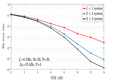
Figure 3: BER performance of MIMO-OTFS for SISO, and $2\times 2$ and $3\times 3$ MIMO systems.

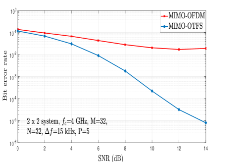
Figure 4: BER performance comparison between MIMO-OTFS and MIMO-OFDM in a $2\times 2$ MIMO system.

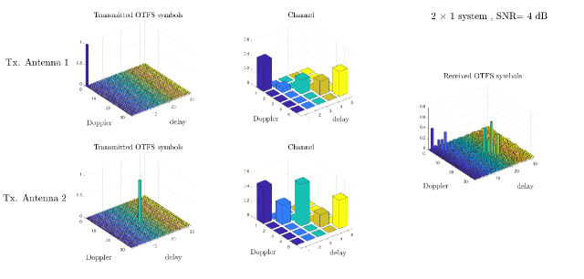
Figure 5: Illustration of pilots and channel response in delay-Doppler domain in a 2$\times$1 MIMO-OTFS system.

Figure 4 shows the BER performance comparison between MIMO-OTFS and MIMO-OFDM in a $2\times 2$ MIMO system. The maximum Doppler spread in the considered system is high (1880 Hz) which causes severe ICI in the TF domain. Because of the severe ICI, the performance of MIMO-OFDM is found to break down and floor at a BER value of about $2\times 10^{-2}$. However, MIMO-OTFS is able to achieve a BER of $10^{-5}$ at an SNR value of about 14 dB. This is because OTFS uses the delay-Doppler domain for signaling instead of TF domain. Thus, the BER plots clearly illustrate the robust performance of MIMO-OTFS and its superiority over MIMO-OFDM under rapidly varying channel conditions.

V Channel Estimation for MIMO-OTFS

In this section, we relax the assumption of perfect channel knowledge and present a channel estimation scheme in the delay-Doppler domain. The scheme uses impulses in the delay-Doppler domain as pilots. Figure 5 gives an illustration of the pilots, channel response, and received signal in a $2\times 1$ MIMO system with the delay-Doppler profile and system parameters given in Tables I and II. Each transmit and receive antenna pair sees a different channel having a finite support in the delay-Doppler domain. The support is determined by the delay and Doppler spread of the channel [8]. This fact can be used to estimate the channel for all the transmit-receive antenna pairs simultaneously using a single MIMO-OTFS frame as described below.

The OTFS input-output relation for $p$th transmit antenna and $q$th receive antenna pair can be written using (12) as

$${\hat{x}}_{q}[k,l]=\sum_{m=0}^{M-1}\sum_{n=0}^{N-1}x_{p}[n,m]{1\over MN}{h_{w_{qp}}}\left({k-n\over NT},{l-m\over M\Delta f}\right)+v_{q}[k,l].$$ (32)

If we transmit

$$x_{p}[n,m] =1\ \text{if}\ (n,m)=(n_{p},m_{p})$$

$$=0\ \forall\ (n,m)\neq(n_{p},m_{p}),$$ (33)

as pilot from the $p$th antenna, the received signal at the $q$th antenna will be

$${\hat{x}}_{q}[k,l]={1\over MN}{h_{w_{qp}}}\left({k-n_{p}\over NT},{l-m_{p}\over M\Delta f}\right)+v_{q}[k,l].$$ (34)

We can estimate ${1\over MN}{h_{w_{qp}}}\left({k\over NT},{l\over M\Delta f}\right)$ from (34), since, being the pilots, $n_{p}$ and $m_{p}$ are known at the receiver a priori. From this, we can get the equivalent channel matrix $\hat{\mathbf{H}}_{qp}$ using the vectorized formulation of Sec. II-C. From (34) we also see that, due to the 2D-convolution input-output relation, the impulse at $(n,m)=(n_{p},m_{p})$ is spread by the channel only to the extent of the support of the channel in the delay-Doppler domain. Thus, if we send the pilot impulses from the transmit antennas with sufficient spacing in the delay-Doppler domain, they will be received without overlap. Hence, we can estimate the channel responses corresponding to all the transmit-receive antenna pairs simultaneously and get the estimate of the equivalent MIMO-OTFS channel matrix $\hat{\mathbf{H}}_{{\tiny\mbox{MIMO}}}$ using a single MIMO-OTFS frame. This is illustrated in Fig. 5 for a $2\times 1$ MIMO-OTFS system with frame size $(M,N)=(32,32)$ at an SNR value of 4 dB. The first antenna transmits the pilot impulse at $(n_{1},m_{1})=(0,0)$ and the second antenna transmits the pilot impulse at $(n_{2},m_{2})=(16,16)$ in the delay-Doppler domain. We observe that the impulse response ${h_{w_{11}}}\left({k-n_{1}\over NT},{l-m_{1}\over M\Delta f}\right)$ and ${h_{w_{12}}}\left({k-n_{2}\over NT},{l-m_{2}\over M\Delta f}\right)$ are non-overlapping at the receiver. Thus, they can be estimated simultaneously using a single pilot MIMO-OTFS frame.

V-A Performance results and discussions

In this subsection, we present the BER performance of the MIMO-OTFS system using the estimated channel. We use the MIMO-OTFS channel estimation scheme described above, for estimating the equivalent channel matrix $\hat{\mathbf{H}}_{{\tiny\mbox{MIMO}}}$ and use the message passing algorithm for detection. The delay-Doppler profile and the simulation parameters are as given in Table I and Table II, respectively.

In Fig. 6, we plot the Frobenius norm of the difference between the equivalent channel matrix (${\mathbf{H}}_{{\tiny\mbox{MIMO}}}$) and the estimated equivalent channel matrix ($\hat{\mathbf{H}}_{{\tiny\mbox{MIMO}}}$) (a measure of estimation error) as a function of pilot SNR for a $2\times 2$ MIMO-OTFS system with system parameters as in Tables I and II. We observe that, as expected, the Frobenius norm of the difference matrix decreases with pilot SNR. Figure 7 shows the corresponding BER performance using the proposed channel estimation scheme for the $2\times 2$ MIMO-OTFS system. It is observed that the BER performance achieved with the estimated channel is quite close to the performance with perfect channel knowledge. For example, a BER of $2\times 10^{-5}$ is achieved at SNR values of about 12.5 dB and 13 dB with perfect channel knowledge and estimated channel knowledge, respectively. At the considered maximum Doppler frequency of 1880 Hz, channel estimation in the time-frequency domain leads to inaccurate estimation because of the rapid variations of the channel in time. On the other hand, the sparse channel representation in the delay-Doppler domain is time-invariant over a larger observation time. This, along with the OTFS channel-symbol coupling (2D periodic convolution) in the delay-Doppler domain, enables the proposed channel estimation for MIMO-OTFS to be simple and efficient.

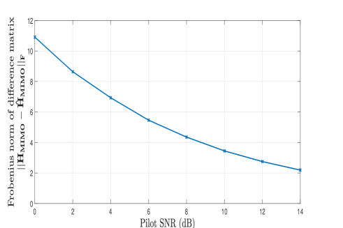
Figure 6: Frobenius norm of the difference between the equivalent channel matrix (${\mathbf{H}}_{{\tiny\mbox{MIMO}}}$) and the estimated equivalent channel matrix ($\hat{\mathbf{H}}_{{\tiny\mbox{MIMO}}}$) as a function of pilot SNR in a 2$\times$2 MIMO-OTFS system.

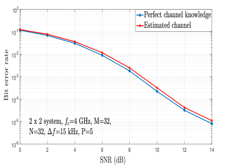
Figure 7: BER performance of MIMO-OTFS system using the estimated channel in a 2$\times$2 MIMO-OTFS system.

VI Conclusions

We investigated signal detection and channel estimation aspects of MIMO-OTFS under high-Doppler channel conditions. We developed a vectorized formulation of the input-output relationship for MIMO-OTFS which enables MIMO-OTFS signal detection. We presented a low complexity iterative algorithm for MIMO-OTFS detection based on message passing. The algorithm was shown to achieve very good BER performance even at high Doppler frequencies (e.g., 1880 Hz) in a $2\times 2$ MIMO system where MIMO-OFDM was shown to floor in its BER performance. We also presented a channel estimation scheme in the delay-Doppler domain, where delay-Doppler impulses are used as pilots. The proposed channel estimation scheme was shown to be efficient and the BER degradation was small as compared to the performance with perfect channel knowledge. The sparse nature of the channel in the delay-Doppler domain which is time-invariant over a larger observation time enabled the proposed estimation scheme to be simple and efficient.

References

- [1] W. C. Jakes, Microwave Mobile Communications, New York: IEEE Press, reprinted, 1994.
- [2] A. Goldsmith, Wireless Communications, Cambridge Univ. press, 2005.
- [3] T. Wang, J. G. Proakis, E. Masry, and J. R. Zeidler, “Performance degradation of OFDM systems due to Doppler spreading,” IEEE Trans. Wireless Commun., vol. 5, no. 6, pp. 1422-1432, Jun. 2006.
- [4] T. Strohmer and S. Beaver, “Optimal OFDM design for time-frequency dispersive channels,” IEEE Trans. Commun., vol. 51, no. 7, pp. 1111-1122, Jul. 2003.
- [5] F-M. Han and X-D. Zhang, “Hexagonal multicarrier modulation: a robust transmission scheme for time-frequency dispersive channels,” IEEE Trans. Signal Process., vol. 55, no. 5, pp. 1955-1961, May 2007.
- [6] F-M. Han and X-D. Zhang, “Wireless multicarrier digital transmission via Weyl-Heisenberg frames over time-frequency dispersive channels,” IEEE Trans. Commun., vol. 57, no. 6, pp. 1721-1733, Jun. 2009.
- [7] R. Hadani and A. Monk, “OTFS: A new generation of modulation addressing the challenges of 5G,” online: arXiv:1802.02623 [cs.IT] 7 Feb 2018.
- [8] A. Monk, R. Hadani, M. Tsatsanis, and S. Rakib, “OTFS - orthogonal time frequency space: a novel modulation technique meeting 5G high mobility and massive MIMO challenges,” online: arXiv:1608.02993 [cs.IT] 9 Aug 2016.
- [9] R. Hadani, S. Rakib, M. Tsatsanis, A. Monk, A. J. Goldsmith, A. F. Molisch, and R. Calderbank, “Orthogonal time frequency space modulation,” Proc. IEEE WCNC’2017, pp. 1-7, Mar. 2017.
- [10] R. Hadani, S. Rakib, A. F. Molisch, C. Ibars, A. Monk, M. Tsatsanis, J. Delfeld, A. Goldsmith, and R. Calderbank, “Orthogonal time frequency space (OTFS) modulation for millimeter-wave communications systems,” in Proc. IEEE MTT-S Intl. Microwave Symp., pp. 681-683, Jun. 2017.
- [11] L. Li, H. Wei, Y. Huang, Y. Yao, W. Ling, G. Chen, P. Li, and Y. Cai, “A simple two-stage equalizer with simplified orthogonal time frequency space modulation over rapidly time-varying channels,” online: arXiv:1709.02505v1 [cs.IT] 8 Sep 2017.
- [12] P. Raviteja, K. T. Phan, Q. Jin, Y. Hong, and E. Viterbo, “Low-complexity iterative detection for orthogonal time frequency space modulation,” online: arXiv:1709.09402v1 [cs.IT] 27 Sep 2017.
- [13] A. R. Reyhani, A. Farhang, M. Ji, R-R. Chen, and B. Farhang-Boroujeny, “Analysis of discrete-time MIMO OFDM-based orthogonal time frequency space modulation,” arXiv:1710.07900v1 [cs.IT] 22 Oct 2017.
- [14] T. Dean, M. Chowdhury, and A. Goldsmith, “A new modulation technique for Doppler compensation in frequency-dispersive channels,” Proc. IEEE PIMRC’2017, Oct. 2017.
- [15] A. Farhang, A. Rezazadeh Reyhani, L. E. Doyle, and B. Farhang-Boroujeny, “Low complexity modem structure for OFDM-based orthogonal time frequency space modulation,” IEEE Wireless Commun. Lett., doi: 10.1109/LWC.2017.2776942, Nov. 2017.
- [16] K. R. Murali and A. Chockalingam, “On OTFS modulation for high-Doppler fading channels,” Proc. ITA’2018, San Diego, Feb. 2018.
- [17] Y.G. Li, J.H. Winters, and N.R. Sollenberger, “MIMO-OFDM for wireless comunications: signal detection with enhanced channel estimation,” IEEE Trans. Commun., vol. 50, no. 9, pp. 1471-1477, Sep. 2002.
- [18] F. Hlawatsch and G. Matz, Wireless Communications Over Rapidly Time-Varying Channels, Academic Press, 2011.
- [19] A. Fish, S. Gurevich, R. Hadani, A. M. Sayeed, and O. Schwartz, “Delay-Doppler channel estimation in almost linear complexity,” IEEE Trans. Inf. Theory, vol. 59, no. 11, pp. 7632-7644, Nov. 2013.