The second law and beyond in microscopic quantum setups

Abstract

The Clausius inequality (CI) is one of the most versatile forms of the second law. Although it was originally conceived for macroscopic steam engines, it is also applicable to quantum single particle machines. Moreover, the CI is the main connecting thread between classical microscopic thermodynamics and nanoscopic quantum thermodynamics. In this chapter, we study three different approaches for obtaining the CI. Each approach shows different aspects of the CI. The goals of this chapter are: (i) To show the exact assumptions made in various derivations of the CI. (ii) To elucidate the structure of the second law and its origin. (iii) To discuss the possibilities each approach offers for finding additional second-law like inequalities. (iv) To pose challenges related to the second law in nanoscopic setups. In particular, we introduce and briefly discuss the notions of exotic heat machines (X machines), and “lazy demons”.

I Introduction

Quantum thermodynamics deals with a broad spectrum of issues related to thermodynamics of small and quantum systems. In particular, this chapter examines the applicability of one the most fundamental ideas in thermodynamics: the second law. In addition to its classical role, the second law is the main connecting thread between classical thermodynamics and thermodynamics of microscopic (possibly highly quantum) systems.

The second law has various formulations. Here we consider one of the most versatile and useful forms: the Clausius inequality

$$\Delta S-\intop\frac{\delta Q}{T}\geq 0,$$ (1)

where $S$ is the entropy of the system, and $Q$ is the heat exchanged with a bath at temperature $T$. In classical thermodynamics, entropy changes are defined by the quantity $\intop\frac{\delta Q}{T}$ evaluated for a reversible process between two equilibrium states. The bath is assumed to be large with a well-defined temperature at all stages of the evolution.

The Clausius equality (CI) is quite remarkable. It provides a quantitative prediction that can easily be adapted to the quantum microscopic world. One of the important results of applying the CI to the microscopic and/or quantum world, is that the efficiency of quantum heat engines is limited by the Carnot efficiency even when the evolution exploits unique quantum properties such as entanglement. The CI also provides a very easy way to understand Szilard engines, and Landauer’s erasure principle (Landauer, 1961; Reeb and Wolf, 2014).

As described later in detail, under reasonable assumptions the CI is well understood, and can be obtained for microscopic systems using several different approaches. However, there are several open questions and challenges related to the CI: (1) Is the current regime of validity sufficiently large to handle important microscopic scenarios? If not, the CI should be further explored and extended. (2) In microscopic setups where the CI is valid, is it also useful? (3) Is the CI a one of a kind constraint, or is it just one member of a family of constraints on microscopic thermodynamic processes? Recent studies show that additional constraints do exist (Brandão et al., 2015; Horodecki and Oppenheim, 2013; Lostaglio et al., 2015; Uzdin, 2017).

The importance of additional constraints or “laws” comes from the fact that in nanoscopic setups, systems are easily taken out of equilibrium. In equilibrium macroscopic systems, knowledge of a few coarse-grained properties (e.g., internal energy, volume, pressure, etc.) is sufficient for knowing almost everything about the system. In contrast, in small out of equilibrium systems, changes in the internal energy, for example, provide only a limited amount of information on how the energy distribution deviates from equilibrium. Moreover, in small systems, it is possible to experimentally probe features that are more detailed than the average energy, e.g., the energy variance. Thus, it is intriguing to ask if there are thermodynamic constraints, perhaps of the CI form, on other moments of the energy (Uzdin, 2017), or on other measurable features of the system. Furthermore, in microscopic setups, the environment itself may be very small. Thus, it is conceivable to measure various environment properties (e.g. energy variance) as the environment starts to deviate from its initial equilibrium state.

In trying to extend the regime of validity of the CI, or in the search of new thermodynamic constraints on new quantities, it is important to keep track on what properties of the CI have been retained, what features have been lost or replaced, and at what cost. In particular, does the extension involve measurable quantities and what is the predictive power of the new suggested extension with respect to present and future experiments. For example, thermodynamic resource theory predicts that there are families of mathematical constraints on a specific set of processes involving thermal baths. This is a very interesting and important finding. However, these constraints do not deal directly with observable quantities and their operational (or informational) meaning has not been clarified yet. It is not a necessary requirement that new constraints will have the same form and nature of the CI. However, it is very interesting to explore and find constraints that resemble the second law and its rock-solid, well-established logic. Thus, this chapter puts emphasis on the structure of the CI, and its various features.

In what follows, we aim to achieve the goals stated in the abstract by studying three different approached to derive the CI: (1) The reduced entropy approach; (2) The global passivity approach; (3) The Completely positive maps approach. Each approach shows different aspects of the CI, and can lead to new challenges related to the second law in nanoscopic setups. Before exploring each approach let us state the CI statement of the second law in microscopic setups.

II The CI in microscopic and quantum setups

Consider a setup that is composed of a system that is initially in an arbitrary mixed or pure state, and several environments that are initially in thermal equilibrium (Gibbs states). All elements (’element’ may refer to the system, or to one of its environments) are initially uncorrelated, so at $t_{0}$ the setup shown in Fig. 1a is described by the following total density matrix (Fig. 1a):

$$\rho_{0}^{tot}=\rho_{0}^{sys}\otimes\frac{e^{-\beta_{1}H_{1}}}{Z_{1}}\otimes\frac{e^{-\beta H_{2}}}{Z_{2}}\otimes...$$ (2)

where $H_{k}$ is the Hamiltonian of environment $k$, $\beta_{k}=1/T_{k}$ is its initial inverse temperature, and the $Z_{i}$’s are normalization factors. We call an environment that is initially prepared in a thermal state a ’microbath’ (later denoted in equations by $\mu b$). Unlike macroscopic baths, microbaths are not assumed to be large and to remain in a thermal state while interacting with the system. The only requirement of a microbath is that its initial state is thermal. That said, the microbath is allowed to be very large. The preparation process of a microbath is outside the scope of the present discussion. We shall assume that such (possibly small) initially thermal environments are given in the beginning of the experiment. Nevertheless, in principle, they can be prepared by weakly interacting with a much larger thermal environment.

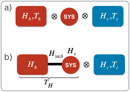
Figure 1: (a) The standard CI form of the second law assumes that all elements are initially uncorrelated (2). (b) In microscopic setups where a system is initially strongly coupled to one of the environments, the system starts in a coupled Gibbs state (50). Hence, in general, the system does not have a thermal form then the environment is traced out. The CI does not hold in this scenario. Nonetheless, new approaches can successfully handle this scenario (Sec. IV.4).

The evolution of the setup is generated by some global time-dependent Hamiltonian that describes all the interactions between the system, the microbaths, and external fields (i.e., driving). In such setups the following microscopic form of the CI (Peres, 2006; Esposito and Van den Broeck, 2011; Sagawa, 2012; Strasberg et al., 2017; Lostaglio et al., 2017; Guryanova et al., 2016; Halpern et al., 2016) holds:

$$\Delta S_{VN}^{sys}+\sum\beta_{k}q_{k} \geq 0$$ (3)

$$q_{k} =\Delta\left\langle H_{k}\right\rangle$$ (4)

where $S_{VN}^{sys}=-tr[\rho^{sys}\ln\rho^{sys}]$ is the von Neumann entropy of the system (we shall drop the VN subscript hereafter). The $\Delta$ always refers to changes with respect to time $t_{0}$ where (2) holds, e.g., at time $t$: $\Delta S^{sys}=S(t)-S(t_{0})$. $q_{k}$ is the heat or more accurately the energy transferred to $k$-th microbath. For $q_{k}$ to represent the energy change in bath k, $H_{k}$ must be satisfy $H_{k}(t_{f})=H_{k}(t_{0})$ which means that at the end of the process the environment is not modified directly by external field (it only interacts with other elements). A classical derivation is carried out in (Jarzynski, 1999; Deffner and Jarzynski, 2013). We point out a few interesting facts on the microscopic CI result (3)

• As long as the initial condition (2) holds, the interaction between the elements and the external driving can be arbitrarily strong and lead to highly non-Markovian dynamics.

• The microbaths and the system can be arbitrary small in size (e.g., a single spin) as long as the initial state of the setup is given by (2).

• The microbath can be very far from thermal equilibrium at the end and during the interaction with the system. The $\beta_{k}$’s refer only to the initial temperatures of the microbath.

For additional refinements of the CI see (Reeb and Wolf, 2014; Deffner and Lutz, 2010). In what follows, we derive (3) using different approaches.

III The reduced entropy approach

For simplicity of notation, let us assume we have only three elements: a system ’$s$’, and two environments ’$A$’ and ’$B$’. At this point, it is not assumed that the environments are initially thermal. However, all three elements are assumed to be initially uncorrelated to each other so the initial density matrix is given by

$$\rho_{0}^{tot}=\rho_{0}^{s}\otimes\rho_{0}^{A}\otimes\rho_{0}^{B}.$$ (5)

Next, we assume that the evolution is generated by some time-dependent Hamiltonian of the form:

$$H_{tot}(t)=H_{s}(t)+H_{A}(t)+H_{B}(t)+H_{int}(t),$$ (6)

where the first term describes possible external driving of the system (e.g. by laser light), the next two terms are the environment Hamiltonians (which may also be subjected to external fields), and the last term describes the time-dependent interactions between the three elements. This generic Hamiltonian can describe almost any thermodynamic protocol that does not involve feedback or measurements during the evolution. No other interactions or other parties are involved. Note that typically the environments ($A$ and $B$) are either not driven $\frac{d}{dt}H_{A(B)}=0$ by external fields, or at the very least are not modified at the end of the thermodynamic protocol

$$H_{A(B)}(t_{f})=H_{A(B)}(t_{0}).$$ (7)

However, this assumption is not needed until Eq. (19).

In quantum mechanics, any $H_{tot}(t)$ leads to a unitary evolution operator $U$ (i.e., $U^{\dagger}U=I$) that relates the final density matrix to the initial one,

$$\rho_{t}^{tot}=U\rho_{0}^{tot}U^{\dagger}.$$ (8)

Finally, we consider a slightly more general case where there is some noise in $H_{tot}(t)$ (this noise can be a control amplitude noise, timing noise, etc) so that with probability $p_{j}$, $U_{j}$ is executed instead of the desired $U$. As a result, the evolution of the setup is described by a mixture of unitaries

$$\rho_{t}^{tot}=\sum p_{k}U_{k}\rho_{0}^{tot}U_{k}^{\dagger}.$$ (9)

Next, we use the non-negativity of the quantum relative entropy (Nielsen and Chuang, 2002) for any two density matrices $\rho$ and $\sigma$

$$D(\rho|\sigma)\doteq\text{tr}[\rho(\ln\rho-\ln\sigma)]\geq 0,$$ (10)

where equality holds if and only if $\rho=\sigma$. We set $\rho$ to be the state of the setup at time t $\rho=\rho_{t}^{tot}$, and $\sigma$ to be the tensor product of the local density matrices $\sigma=\rho_{t}^{s}\otimes\rho_{t}^{A}\otimes\rho_{t}^{B}$ where $\rho_{t}^{(i)}\doteq\text{tr}_{\neq i}[\rho_{t}^{tot}]$. Using the log property for product states ($\sigma$), we get

$$D(\rho_{t}^{tot}|\rho_{t}^{s}\otimes\rho_{t}^{A}\otimes\rho_{t}^{B})=(\sum_{j=s,A,B}S_{t}^{j})-S_{t}^{tot}\geq 0,$$ (11)

where the inequality follows from the non negativity of the quantum relative entropy (10). If the global evolution is unitary (8), then $S_{t}^{tot}=S_{0}^{tot}$ since all the eigenvalues of the total density matrix are conserved quantities. If the global evolution is a mixture of unitaries (9) then due to the Schur concavity (Marshall et al., 1979) of the von Neumann entropy it holds that,

$$S_{t}^{tot}\geq S_{0}^{tot}.$$ (12)

Note that this inequality is not a manifestation of the second law. Unlike the inequality (11) that holds also for a unitary evolution, the one in (12) originates from the randomness/noise in the protocol that we have included for generality. Using (12) in (11) we get

$$(\sum_{j=s,A,B}S_{t}^{j})-S_{0}^{tot}\geq 0.$$ (13)

Since the setup starts in a product state (5) it holds that $S_{0}^{tot}=\sum_{j=s,c,h}S_{0}^{j}$ and (13) becomes the reduced entropy growth form of the (microscopic) second law (Peres, 2006; Esposito and Van den Broeck, 2011; Sagawa, 2012),

$$\sum_{j=s,c,h}\Delta S^{j}\geq 0.$$ (14)

This form is strictly entropic and has no reference to heat or energy. Moreover, (14) holds even if the environments are initially in highly non-thermal states. For two parties, (14) can be obtained from the non-negativity of the quantum mutual information (Nielsen and Chuang, 2002). When there are more parties, (11) should be used.

Equation (14) has the following information interpretation. For any global unitary the total entropy is conserved $\Delta S^{tot}=0$. However, the final density matrix contains classical and quantum correlations between the different elements. The sum of reduced entropies does not include these correlations, and therefore it grows despite the fact that the total entropy is conserved.

It is important to highlight several points. (1) This growth is only with respect to the initial values, and the growth is typically non-monotonic in time due to the possible non-Markovian nature of the evolution. (2) The reason the entropy is growing and not decreasing is due to the special assumption that the elements are initially uncorrelated. (3) As mentioned earlier, no assumptions were made on the size of the elements. The bath or the system can be as small as a single spin. These features make the entropic form of the second law useful for understanding processes involving small quantum systems (e.g., algorithmic cooling (P. Oscar Boykin, Tal Mor, Vwani Roychowdhury, Farrokh Vatan, and Rutger Vrijen, 2002)).

III.1 The Clausius inequality: the energy-information form of the second law

The transition from the entropic form of the second law to the energy-information CI form, involves three more simple steps. The first is to apply the following identity that holds for any two density matrices $\rho_{1},\rho_{2}$.

$$S(\rho_{2})-S(\rho_{1})\equiv\text{tr}[(\rho_{2}-\rho_{1})(-\ln\rho_{1})]-D(\rho_{2}|\rho_{1}).$$ (15)

Applying this identity to the initial and final reduced states of the $k$-th environment

$$\Delta S^{env,k}=\Delta\left\langle-\ln\rho_{0}^{env,k}\right\rangle-D(\rho_{f}^{k}|\rho_{0}^{k}),$$ (16)

and substituting it in (14) we obtain

$$\Delta S^{sys}+\sum_{k}\Delta\left\langle-\ln\rho_{0}^{env,k}\right\rangle\geq\sum_{k}D(\rho_{f}^{k}|\rho_{0}^{k}).$$ (17)

The next step is to set the environments to be microbaths, i.e. $\rho_{0}^{env,k}\to\rho_{0}^{\mu b,k}=e^{-\beta_{k}H_{k}^{\mu b}}/Z_{k}$ and get

$$\Delta S^{sys}+\sum_{k}\beta_{k}q_{k}\geq\sum_{k}D(\rho_{f}^{\mu b,k}|\rho_{0}^{\mu b,k}),$$ (18)

where, as before, we denote the change in the average energy of bath $k$ by $q_{k}$

$$q_{k}\doteq\text{tr}[(\rho_{f}^{\mu b,k}-\rho_{0}^{\mu b,k})H_{k}^{\mu b}].$$ (19)

In interpreting $q_{k}$ as the change in the energy of the bath we use assumption (7). Due to the the relative entropy terms in (18), form (18) is slightly stronger than the standard CI (3). However, the relative entropy terms cannot be easily measured. Nevertheless, they are not void of physical meaning. They represent the work that can be extracted from the microbaths due to the fact they are not in a thermal state at the end of the process. If, for example, an additional auxiliary large bath at temperature $T_{h}$ was available, then a $T_{h}D(\rho_{f}^{\mu b,h}|\rho_{0}^{\mu b,h})$ amount of work could have been reversibly extracted from the hot microbath. However, since we consider an entropically self-contained setups (where a large external bath is not included), this work extraction scheme is irrelevant.

In the last third step, the relative entropy property $D(\rho_{f}^{k}|\rho_{0}^{k})\geq 0$ is used to obtain the CI inequality (3) from (18). Finally, by defining the operator

$$B^{env} =-\ln\rho_{0}^{env},$$ (20)

where $\rho_{0}^{baths}$ is the initial density matrices of all the microbaths in the setup, the CI can be written more compactly as

$$\Delta S^{sys}+\Delta\left\langle B^{env}\right\rangle\geq 0.$$ (21)

This form will be used in Sec. IV.4.

III.2 The structure of the CI

The CI connects two very different quantities. One is an information measure, and the other is an expectation value obtained from energy measurements. These two quantities have completely different nature and properties. $S^{sys}(\rho^{sys})$ is an information measure and as such it is nonlinear in $\rho_{sys}$. It is basis-independent, and invariant to permutations and unitary transformation: $S^{sys}(\rho^{sys})=S^{sys}(U\rho^{sys}U^{\dagger})$. That is, only the eigenvalues of the density matrix are important. It matters not to which orthogonal states these eigenvalues are assigned. $S^{sys}(\rho^{sys})$ quantifies the ignorance about the system. If it is in a known pure state $\left|\psi\right\rangle$ then $S^{sys}(\left|\psi\right\rangle\left\langle\psi\right|)=0$. If $\rho^{sys}$ is in a fully mixed state then $S^{sys}$ obtains a maximal value.

The second term in the CI $\beta q=\beta\Delta\left\langle H_{\mu b}\right\rangle$ is completely different. First, it is linear in the density matrix. Second, it is not invariant under permutations and more general unitary transformations $tr[U\rho^{\mu b}U^{\dagger}H^{\mu b}]\neq tr[\rho^{\mu b}H^{\mu b}]$. Moreover, $\left\langle H^{\mu b}\right\rangle$ involves only the diagonal elements of the density matrix in the energy basis. Thus, dephasing all the coherences in the energy basis will not change the energy expectation values at a given instant (it will, however, change the evolution from that point on). In contrast, information quantities such as the von Neumann entropy are very sensitive to dephasing. All types of dephasing operations increase the values of $S^{sys}(\rho^{sys})$. We point out that all Schur concave information measures have this property (Marshall et al., 1979; Uzdin, 2017).

This relation between a quantity that is basis-independent and a quantity that is basis-dependent can be quite powerful. For example, if we erase one bit of information from our system (no matter in which basis), then according to the CI (Landauer principle (Landauer, 1961; Reeb and Wolf, 2014)) at least $T\ln 2$ amount of heat has to be exchanged with the bath. Thus, although nonlinear quantities such as $S^{sys}(\rho^{sys})$ are not directly measurable (they are not associated with an Hermitian operator), they can be quite insightful when associated with expectation values as in the CI. Note that in the CI the nonlinear quantities involve only the system, which at least in nanoscopic setups can be regarded as small. For example, it is not unreasonable to perform tomography of a two-spin system, if needed. On the other hand, it not practical to perform a full tomography of a thirty-spin microbath in order to evaluate its entropy changes. Hence, when using nonlinear quantities in thermodynamics, we should be mindful how they can be evaluated or used either directly or indirectly.

Finally, we point out that a major feature of the CI is that the inequality is saturated (becomes an equality) for reversible processes. This saturation is highly important for two main reasons. First, inequalities that are not saturated can be completely useless. For example, $\Delta S+\beta q+10^{100}\geq 0$ is also a valid inequality, but it is trivially satisfied and cannot be used to state something useful on $\Delta S$ by knowing $q$ or vice versa. The second reason why the CI saturation is important is that it provides a special meaning to reversible processes compared to irreversible processes. All reversible processes between two endpoints (two density matrices of the systems) are equivalent in terms of heat, work, and entropy changes in the bath. On the other hand, irreversible processes are path-dependent and lead to suboptimal work extraction. As a side note, we point out that creating a reversible interaction with microbaths is not as straightforward as it is in macroscopic setups since, in general, the microbaths do not remain in a Gibbs state.

III.3 Fluctuation theorems and Clausius-like inequalities

Fluctuation theorems (FT’s) are intensively studied for the last few decades (see reviews (Jarzynski, 2011; Speck and Seifert, 2007; Harris and Schütz, 2007)). Their main appeal is that they provide equalities that hold even when the system is driven far away from equilibrium. In contrast, the CI provides a potentially saturated inequality in non-equilibrium dynamics.

Interestingly, by applying mathematical inequality (Jensen inequality), some manifestations of the CI can be retrieved from FT’s. For this reason, it is sometimes claimed that FT’s are more fundamental than the CI. However, it is highly important to remember that, presently, the CI is applicable in various scenarios where FT’s may not hold or become impractically to use: (1) Initial coherence in the energy eigenbasis of the systems. (2) Interaction with microbaths that substantially deviate from thermal equilibrium during the evolution so that detailed balance does not hold anymore. In addition, FT’s yields the a weaker form of the second law which is based on the equilibrium entropy (equilibrium free energy) and not in terms of von Neumann entropy of the final non-equilibrium state (non-equilibrium free energy (30)). Moreover, treating multiple bath in FT’s, as in the CI, is also a non trivial matter. In particular, the observed quantity is no longer work (Campisi et al., 2015).

In summary, in comparison to the CI, fluctuation theorems presently provide stronger statements (equalities) but for more limited physical scenarios. Further study is needed to understand if there is a fundamental complementarity between the strength of non-equilibrium results (FT or CI) and their regime of validity, or perhaps it is possible to hold the stick at both ends and find FT’s that are both more general and stronger than the CI.

Finally, we point that energy appears in the CI in the form of “difference of averages” $q=\left\langle H_{\mu b}\right\rangle_{f}-\left\langle H_{\mu b}\right\rangle_{0}$, while in FT (e.g. (Jarzynski, 1997; Campisi et al., 2015)) energy appears as “ nonlinear average of differences”, e.g., $\left\langle e^{-\beta(E_{f}-E_{0})}\right\rangle$ where $E_{f}$ and $E_{0}$ are initial and final energy measurements in a specific realization (trajectory) (Jarzynski, 1997). That is, the energy term in the CI has the structure $\Delta\left\langle g(H)\right\rangle$ while in FT’s the structure is $\left\langle\tilde{g}(\Delta E)\right\rangle$ where $g$ and $\tilde{g}$ are some analytic functions. In FT’s the evaluation of $\Delta E$ involves measuring $E_{0}$ and $E_{f}$ at the same run of the experiment. In quantum mechanics $E_{0}$ measurements will modify the evolution due to the loss of coherence (wavefunction “collapse”). In contrast, quantities such $\left\langle g(H)\right\rangle_{f}$ and $\left\langle g(H)\right\rangle_{0}$ are evaluated in different runs of the experiment: in one set experimental runs $\left\langle g(H)\right\rangle_{0}$ is measured and evaluated, and in another set of runs $\left\langle g(H)\right\rangle_{f}$ is measured. Therefore, the structure of $\Delta\left\langle g(H)\right\rangle$ is more compatible with quantum mechanics compared to $\left\langle\tilde{g}(\Delta E)\right\rangle$ that appears in FT’s.

III.4 Deficiencies and limitations of the CI

Despite its great success and its internal consistency, the CI also has a few deficiencies. One deficiency concerns very cold environments and the other occurs in dephasing interactions. These deficiencies are not inconsistencies but scenarios where the CI provides trivial and useless predictions.

In the limit of a very low temperature, the predictive power of the Clausius inequality is degraded. As $T=\frac{1}{\beta}\to 0$, the $\beta q$ term diverges and the changes in the entropy of the system becomes negligible (the entropy changes in the system are bounded by the logarithm of the system’s Hilbert dimension). Hence, in this limit, the CI reads $\beta q\geq 0$, which means that heat is flowing into this initially very cold bath. This is hardly a surprise. If the initial temperature is very low the microbath will be in the ground state. Thus, it is clear that any interaction with other agents can only increase its average energy.

Another trivial, and somewhat useless prediction of the CI is obtained in dephasing interactions. Such interactions satisfy $[H_{int},H_{sys}]=0$ and typically also $[H_{int},H_{env}]=0$. Consequently, dephasing interactions do not affect the energy distributions of the system and the environment. However, they degrade the coherence in the energy basis of the system. Since there is no heat flow involved, the CI predicts $\Delta S^{sys}\geq 0$. This is a trivial result: any dephasing process can be written as a mixture of unitaries operating on the system only, and mixture of unitaries always increases the entropy due to the concavity of the von Neumann entropy.

In addition to these two deficiencies, two more obvious deficiencies should be mentioned. The first is the restriction to initially uncorrelated system and environment. In some important microscopic scenarios, this assumption is not valid. This is not a limitation of the derivation in III.1 since in the presence of an initial correlation it is easy to find scenarios which indeed violates the CI (e.g., (Micadei et al., 2017)). Another limitation of the CI is that in some cases it does not deal with the quantities of interest. For example in Sec. VI.3 we discuss machines whose output cannot be expressed in terms of average energy changes or entropy changes. Hence, the CI does not impose a performance limit for these machines.

III.5 The passive CI form: environment energy vs. heat

In this chapter we refer to $q$, the energy exchanged with the bath, as heat. However, this terminology ignores the fact that the microbath can be in a non-passive state that admits work extraction by applying a local unitary on the microbath. Moreover, some studies suggested using ’squeezed thermal bath’ as fuel for quantum heat machines (Roßnagel et al., 2014; Manzano et al., 2015; Maslennikov et al., 2017). A squeezed microbath is obtained by applying a unitary $U_{\mu b}$ to a microbath $\rho_{\beta,sq}^{\mu b}=U_{\mu b}\rho_{\beta}^{\mu b}U_{\mu b}^{\dagger}$. Since the thermal state has the lowest average energy for a given von Neumann entropy, any squeezing operation of a thermal state increases the energy of the bath. Thus, the preparation of squeezed baths requires the consumption of external work.

Next, we use similar arguments to those in (Niedenzu et al., 2018) to show that squeezing can be fully captured in a slightly modified version of the CI. For this, we need to introduce the notion of passive states, ergotropy, and passive energy (Niedenzu et al., 2018). A passive state (passive density matrix) with respect to a Hamiltonian is one in which lower energy states are more populated than higher energy states. In addition, the passive density matrix has no coherences in the energy basis of the Hamiltonian. These states are called passive states since no transient local unitary (acting on the system alone) can reduce the average energy of a system prepared in this state. That is, no work can be extracted from such a state if at the end of the process the system Hamiltonian returns to its initial value (transient unitary). Passive states are discussed in detail in Sec. IV.1 and IV.2.

The maximal amount of work that can be extracted using local transient unitaries is called ergotropy (A. E. Allahverdyan, R. Balian, and Th. M. Nieuwenhuizen, 2004). It is obtained by bringing a non-passive distribution into its passive form with respect to the Hamiltonian. Let $\mathcal{E}$ denote the ’passive energy’ (Niedenzu et al., 2018) that is defined as the energy that remains after extracting all the ergotropy. It is the energy of the passive state associated with some initial non-passive state. Since unitaries do not change the eigenvalues of the density matrix, the initial non-passive state dictates the eigenvalues of the passive state. Therefore, the initial state uniquely determines the passive state up to degeneracies in the Hamiltonian. These possible degeneracies are not important in the present chapter.

The entropic form of the CI (14) holds regardless of squeezing, since squeezing is a local operation that does not change the local entropies. Applying unitary invariance of the VN entropy to squeezed microbaths we can write

$$\Delta S^{\mu b}=S(\rho_{f}^{\mu b})-S(\rho_{sq}^{\mu b}),$$ (22)

as

$$\Delta S^{\mu b} =S(U_{f}\rho_{fin}^{\mu b}U_{f}^{\dagger})-S(U_{i}\rho_{sq,\beta}^{\mu b}U_{i}^{\dagger})$$

$$= S(\rho_{f,pass}^{\mu b})-S(\rho_{\beta}^{\mu b}),$$ (23)

where $U_{f}$ is the unitary that takes the final state of the microbath into a passive state, and $U_{i}$ is the unitary that takes the initial state of the microbath to a thermal passive state. Using (14) and (15) for $\rho_{f,pass}^{\mu b}$ and $\rho_{\beta}^{\mu b}$ we obtain the passive form of the CI (Niedenzu et al., 2018)

$$\Delta S^{sys}+\sum\beta_{k}\Delta\mathcal{E}_{k}\geq 0,$$ (24)

where $\beta_{k}$ is the initial temperature of the unsqueezed $k$-th microbath, and $\mathcal{E}_{k}$ is the passive energy of the $k$-th microbath. One can argue that $\Delta\mathcal{E}_{k}$ is a more accurate definition of heat compared to $\Delta\left\langle H_{k}\right\rangle$ as it excludes ergotropy. However, another point of view is that heat is related to energy that cannot be operationally extracted in practice. If retrieving the ergotropy from the bath is too complicated to implement then for all practical purposes all energy dumped into the microbath can be considered as heat. For macroscopic baths, direct work on the bath is usually not considered as it may often involve keeping track of phases of many interacting degrees of freedom. However, in the microscopic world where the size of the microbath may be comparable to that of the system, work extraction from a microbath is not an unreasonable operation. In conclusion, the decision whether to use (3) or (24) may strongly depend on the experimental capabilities in a specific setup.

That said, one of the nice features of the CI (3) is that it does not depend on heat and work separation or interpretation. It simply puts a limit on the changes in the average energy of the microbaths. Work and heat separation and the very definition of work becomes very obscure, and to some extent immaterial, when trying to define higher moments of work in the presence of initial coherences in the energy basis (see, for example, Ref. (Perarnau-Llobet et al., 2017)). On the other hand, changes in higher moments of the energy of the system are well defined even in the presence of initial coherences (see Sec. III.3). This is exploited in (Uzdin, 2017). See (Niedenzu et al., 2018; Bera et al., 2017) for schemes that suggest some alternative separations of heat and work.

III.6 Quantum coherence and the Clausius inequality

The microscopic form of the CI (3) is so similar to the historical macroscopic form put together by Clausius (1), that one may wonder if (3) contains any quantum features at all. The difference between stochastic dynamics of energy population and quantum dynamics manifests in ’coherences’: the off-diagonal elements of the density matrix that quantify quantum superposition of energy states. Coherence and its quantification is actively studied in recent years(Streltsov et al., 2017).

Removal of the system coherence by some process increases the entropy of the system. According to the CI the growth of entropy sets a bound on how much heat can be exchanged in such a decoherence process that affects only the off diagonal elements of the density matrix. Indeed, as discussed in Sec. III.4 by using a specific type of system-environment dephasing interactions it is possible to decohere the system without changing the energy of the system or the microbath (no heat flow). This thermodynamically irreversible process involves significant correlation buildup between the system and the microbath (Uzdin and Rahav, 2018). However, in Ref. (Kammerlander and Anders, 2016) a protocol was suggested to remove the coherence in a reversible process.

The Kammerlander-Anders protocol (Kammerlander and Anders, 2016) reversibly implements $\rho_{i}\to\text{diag}(\rho_{i})$ in two stages. In stage $I$, a unitary transformation is applied to the system, and brings it into an energy diagonal state. This step involves work without any entropy changes $S_{I}^{\prime}=S_{I}=S(\rho_{i})$. In stage $II$ a standard reversible diagonal/stochastic state preparation protocol is employed to change $\text{diag}(\rho^{\prime})$ to $\text{diag}(\rho_{i})$. The entropy change in this stage is

$$\Delta S_{II}=S[\text{diag}(\rho_{i})]-S_{I}^{\prime}=S[\text{diag}(\rho_{i})]-S(\rho_{i}).$$ (25)

Note that this expression is always positive as it can be written in terms of quantum relative entropy

$$\Delta S_{II}=S[\text{diag}(\rho_{i})]-S(\rho_{i})=D[\rho_{i}|\text{diag}(\rho_{i})]\geq 0.$$ (26)

The heat required to reversibly generate this entropy difference using a single-bath is given by the CI

$$q^{rev}=-T\Delta S_{II}.$$ (27)

Since the initial and final average energy are the same (same values of the diagonal elements, and the same Hamiltonian) it follows that the work in this reversible process is

$$W^{rev}=q^{rev}=TD[\rho_{i}|\text{diag}(\rho_{i})]\geq 0.$$ (28)

Since the CI dictates $q\geq q^{rev}$ it follows that $W^{rev}\geq W$. This result means that work can always be extracted by reversibly removing the coherence in a reversible way. Moreover, reversible protocols extract the maximal amount of work from coherences. Using the CI it was not necessary to describe the protocol in full detail (see (Kammerlander and Anders, 2016; Uzdin, 2017)) to obtain the optimal work extraction.

Another way to think of the thermodynamic role of coherence in the energy basis is to define the non-equilibrium free energy (Still et al., 2012; Esposito and Van den Broeck, 2011) $\mathcal{F}$ through the Clausius inequality (3). Starting with the CI

$$\Delta(S+\beta\Delta\left\langle H^{\mu b}\right\rangle)\geq 0,$$ (29)

and using energy conservation $W+\Delta\left\langle H^{\mu b}\right\rangle+\Delta\left\langle H^{sys}\right\rangle=0$ (no initial or final interaction terms), we get the non-equilibrium free energy form of the CI

$$W \leq-\Delta\mathcal{F},$$ (30)

where $\mathcal{F}=U-TS$ is the non-equilibrium free energy. As in the CI, (30) becomes equality for reversible processes. Since $S[diag(\rho^{sys})]\geq S(\rho^{sys})$, (30) predicts that in a reversible coherence removal process the extracted work is $W=-T\{S(\rho^{sys})-S[diag(\rho^{sys})]\}>0$ as obtained by the KA protocol described above.

Based on the derivations in the last two sections, we can add two more items to CI properties listed in Sec. II

• The passive CI can handle squeezed thermal baths.

• System coherences are taken into account, and play an important role in the microscopic CI.

IV Global passivity approach

IV.1 Traditional passivity and work extraction

Passivity was broadly used in thermodynamics in the context of work extraction (Pusz and Wornwicz, 1978; Lenard, 1978; A. E. Allahverdyan, R. Balian, and Th. M. Nieuwenhuizen, 2004; Niedenzu et al., 2018). We start with the definition of passivity, and then exploit it in new ways (Uzdin and Rahav, 2018). Consider a system subjected to a transient pulse

$$H(t)=H_{0}+H_{pulse}(t).$$

The pulse satisfies $H_{pulse}(t\leq 0;t\geq\tau_{pulse})=0$ so after time $\tau_{pulse}$, the Hamiltonian returns to its initial form. However the final density matrix is modified $\rho_{f}\neq\rho_{0}$ due to non-adiabatic coupling the pulse induced. Since this Hamiltonian generates a unitary transformation, all eigenvalues of the initial density matrix $\lambda(\rho_{0})$ must be conserved (in particular, the entropy is conserved). To maximize the amount of average energy the pulse is extracting from the system (work) we want to minimize the quantity

$$\Delta\text{$\left\langle H_{0}\right\rangle$=}\text{tr}[\rho_{f}H_{0}]-\text{tr}[\rho_{0}H_{0}].$$ (31)

The second term is fixed by the initial condition, so the first term $\text{tr}[\rho_{f}H_{0}]$ has to be minimized. Since the eigenvalues are conserved $\lambda(\rho_{f})=\lambda(\rho_{0})$, the minimal value of $\text{tr}[\rho_{f}H_{0}]$ is obtained by making $\rho_{f}$ diagonal in the energy basis and assigning lower energies with higher eigenvalues of the density matrix (probabilities). This is called the passive distribution. Writing $\lambda_{1}^{\downarrow}\geq\lambda_{2}^{\downarrow}\geq\lambda_{3}^{\downarrow}...$ the passive density matrix with respect to the Hamiltonian is

$$\rho_{pass}=\sum_{k}\lambda_{k}^{\downarrow}\left|k^{\uparrow}\right\rangle\left\langle k^{\uparrow}\right|$$

where $\left|k^{\uparrow}\right\rangle$ are the eigenstates of $H_{0}$ sorted in energy-increasing order $E_{k}\leq E_{k+1}\leq E_{k+2}...$ Alternatively stated, for a system starting in a passive state $\rho_{pass}$ with respect to $H_{0}$ it holds that

$$\Delta\left\langle H_{0}\right\rangle_{pass\to fin}=\text{tr}[\rho_{f}H_{0}]-\text{tr}[\rho_{pass}H_{0}]\geq 0,$$ (32)

for any transient unitary (pulse-like operation). Moreover, from linearity, (32) also holds for any mixture of unitaries (9). As mentioned earlier, the maximal amount of work that can be extracted from an initial state using a transient unitary process is called ergotropy (A. E. Allahverdyan, R. Balian, and Th. M. Nieuwenhuizen, 2004) and is equal to

$$erg=-(\text{tr}[\rho_{pass}H_{0}]-\text{tr}[\rho_{0}H_{0}])\geq 0.$$

Thermal states are passive with respect to the Hamiltonian, but not all passive states are thermal. It turns out that the relationship between thermal states and passive states has a more profound aspect. For a given Hamiltonian $H_{0}$ there are many possible passive states (if $\rho_{0}$ is not specified as it was above). However, thermal states are the only completely passive states. That is, when taking any number $n$ of uncorrelated copies in a thermal state $\rho_{tot}=\rho_{\beta}^{\otimes n}$ then $\rho_{tot}$ is always passive with respect to the total Hamiltonian $H_{0}\otimes I\otimes I..+I\otimes H_{0}\otimes I...+...$ ($I$ is the identity operator). In particular, the thermal state is the only state that remains passive in the limit $n\to\infty$. This is a very important property from the point of view of the second law. If the thermal state was not completely passive then by joining many identical thermal microbaths we could have obtained a non-passive state, and extract work from it, which is in contradiction to the second law.

IV.2 Global passivity

It is important to understand that passivity is not a property of a state $\rho$ or of an operator $\mathcal{A}$, it is a joint property of the pair $\{\rho,\mathcal{A}\}.$ While passivity was traditionally used to describe work extraction of from a system, in (Uzdin and Rahav, 2018) it was suggested that passivity is a much more general concept that can be used for other operators (not just Hamiltonians) and to other objects (not just the system). Based on these observation it was shown in (Uzdin and Rahav, 2018) that passivity plays a much more significant role in thermodynamics compared to the way it was used thus far.

First, we point out that there is no reason to limit passivity to be with respect to the Hamiltonian of the system or the bath. The definition above is applicable to any observable described by an Hermitian operator. For example given a state $\rho_{0}$ in some basis one can ask what is the passive state with respect to the angular momentum operator. In what follows, not only that we will not use passivity with respect to the Hamiltonian, we will also use observables (operators) that involve the whole setup.

Second, usually in the context of passivity, $\mathcal{A}$ is given (the Hamiltonian of the system or of a microbath), and the focus is on the passive state associated with it (Pusz and Wornwicz, 1978; Lenard, 1978; A. E. Allahverdyan, R. Balian, and Th. M. Nieuwenhuizen, 2004; Perarnau-Llobet et al., 2015a, b; Niedenzu et al., 2018). In (Uzdin and Rahav, 2018) it was suggested to look on the opposite problem. Given an initial state (which may not be passive with respect to the Hamiltonian), what are the passive operators with respect to this state? That is, what are the $\mathcal{A}$’s such that $\Delta\left\langle\mathcal{A}\right\rangle\geq 0$ for any (transient) unitary transformation (8) or a mixture of unitaries (9)?

Let $\rho_{0}^{tot}$ be the density matrix that describes the total setup (system plus microbaths). A thermodynamic protocol is a sequence of unitary operations that describe system-environment interaction and interaction with external fields (e.g. a laser field) that act as work repositories. The accumulated effect of this protocol is given by a global unitary $U$ or by a mixture of unitaries (9).

Global passivity (Uzdin and Rahav, 2018) is defined as follows: An operator $\mathcal{B}$ is globally passive (with respect to $\rho_{0}^{tot}$), if it satisfies

$$\Delta\left\langle\mathcal{B}\right\rangle\geq 0,$$ (33)

for any thermodynamic protocol (for any $p_{k}$, and $U_{k}$ in (9)).

As we shall see for any initial preparation $\rho_{0}^{tot}$ there are many families of globally passive operators. To systematically find the passive operators associated with $\rho_{0}^{tot}$ we can use the fact that in thermodynamic setup $\rho_{0}^{tot}$ is explicitly known (in contrast to $\rho_{f}^{tot}$) and construct operators from it. The simplest choice with strongest kinship to the CI is

$$\mathcal{B}^{tot}=-\ln\rho_{0}^{tot}.$$ (34)

We emphasize that this is a time-independent operator and it is linear in the instantaneous density matrix $\rho_{t}^{tot}$. That is, the expectation value at time $t$ is $\left\langle\mathcal{B}^{tot}\right\rangle_{t}=\text{tr}[\rho_{t}^{tot}(-\ln\rho_{0}^{tot})]$. It is easy to verify that this operator is globally passive. According to (34) the probability of observing an eigenvalue $\lambda_{\mathcal{B}}$ is $p_{\lambda_{\mathcal{B}}}=e^{-\lambda_{\mathcal{B}}}$. Hence, larger eigenvalues are associated with lower probabilities and we can conclude that $\rho_{0}^{tot}$ and $\mathcal{B}^{tot}$ form a passive pair, and therefore

$$\Delta\left\langle\mathcal{B}^{tot}\right\rangle\geq 0,$$ (35)

for any mixture of unitaries (9). The connection of the global passivity inequality (35) to the standard CI will be explored in the next section. However, a major difference already stands out: in contrast to the CI (35) holds for any initial $\rho_{0}^{tot}$ even if the system and microbaths are all initially strongly correlated. Thus, (35) has the potential to go beyond a mere re-derivation of the CI.

IV.3 The observable-only analog of the CI

To see the first connection between (35) and the CI we assume the standard thermodynamics assumption on the initial preparation (2) and get that relation (35) now reads

$$\Delta\left\langle\mathcal{B}^{sys}\right\rangle+\sum_{k}\beta_{k}q_{k} \geq 0,$$ (36)

where $\mathcal{B}^{sys}$ is a time-independent operator

$$\mathcal{B}^{sys}\doteq-\ln\rho_{0}^{sys},$$ (37)

and as in Sec. III.1 $q_{k}=\Delta\left\langle H_{k}\right\rangle$ is the change in the average energy of the ${}^{\prime}k^{\prime}$-th bath. Form (36) is linear in the final density matrix and involves only expectations values. Equation (36) looks similar to the CI (3), but instead of the change in the entropy $\Delta S^{sys}$, there is a change in the expectation value of the operator $\mathcal{B}^{sys}.$ Before doing the comparison it is important to point out that in cases we have only microbaths and no system (e.g. in absorption refrigerator tricycles (Amikam Levy and Ronnie Kosloff, 2012), or in a simple bath-to-bath heat flow) then both (36) and the CI reduce to $\sum_{i}\beta_{i}q_{i}\geq 0$. To quantitatively compare the standard CI and (36) in the general case, we use (15) to rewrite (36) as

$$\Delta S^{sys}+\sum_{k}\beta_{k}q_{k}\geq-D(\rho_{f}^{sys}|\rho_{0}^{sys}).$$ (38)

The term on the right-hand side is negative, which means that (36) is a weaker inequality compared to the CI. Nonetheless, (36) has an important merit. To experimentally evaluate $\Delta S^{sys}$ a full system tomography is needed ( $S_{f}^{sys}$ is calculated from $\rho_{f}^{sys}$). In contrast, for $\Delta\left\langle\mathcal{B}^{sys}\right\rangle$ we need to measure only the expectation value of $\mathcal{B}^{sys}$. Not only that this involves only $N$ elements out of the full $N\times N$ density matrix of the system, the elements (probability in the basis of $\mathcal{B}^{sys}$) need not be known explicitly. The average $\left\langle\mathcal{B}^{sys}\right\rangle$ converges much faster compared to evaluation/estimation of the individual probabilities via tomography.

IV.4 CCI - Correlation compatible Clausius inequality

To get the full energy-information form of the CI (3), and to go beyond the standard validity regime (2), we introduce the notion of strong passivity-divergence relation (Uzdin and Rahav, 2018). We start by writing the identity (15) for the whole setup

$$\Delta\left\langle\mathcal{B}^{tot}\right\rangle\equiv\Delta S^{tot}+D(\rho_{f}^{tot}|\rho_{0}^{tot})$$ (39)

where $\mathcal{B}^{tot}$ is defined in (34). When a specific protocol described by a global unitary $U$ is applied to the setup, then $\Delta S^{tot}=0$ since the eigenvalues of the total density matrix do not change in a unitary evolution. What if we have some noise in our controls that implements $U$ and the evolution is described by a mixture of unitaries? In this case it holds that

$$\Delta S^{tot}\geq 0.$$ (40)

This result can be obtained from the concavity of the von Neumann entropy:

$$S(\rho_{f}^{tot}) =S(\sum p_{k}U_{k}\rho_{0}^{tot}U_{k}^{\dagger})\geq$$

$$\sum_{k}p_{k}S(U_{k}\rho_{0}^{tot}U_{k}^{\dagger})=S(\rho_{0}^{tot}).$$ (41)

Property (40) is not unique to the von Neumann entropy, it holds for any Schur concave function (Marshall et al., 1979). A density matrix created by a mixture of unitaries ($\rho_{f}^{tot}$) is majorized by the initial density matrix $\rho_{f}^{tot}\prec\rho_{0}^{tot}$. Therefore, for any Schur concave function $\mathcal{S}$, it holds that $\mathcal{S}$($\rho_{f}^{tot})\geq\mathcal{S}(\rho_{0}^{tot})$ (Marshall et al., 1979). Equation (40) should not be confused with (14) that describes the increase of the sum of reduced entropies when starting from uncorrelated state. While (14) contains the essence of the standard CI, (40) describes another layer of irreversibility created by the noise in the protocol. As we shall see shortly the CI will be obtained from (39) even when there is no randomness in the protocol and $\Delta S^{tot}=0$.

Using (40) in (39), we obtain the ’passivity-divergence relation’

$$\Delta\left\langle\mathcal{B}^{tot}\right\rangle\geq D(\rho_{f}^{tot}|\rho_{0}^{tot}).$$ (42)

This inequality can be viewed as a stronger version of passivity for the following reasons: First, global passivity (35) immediately follows from (42) due to the non-negativity of the quantum relative entropy. Second, (42) implies that the change in the expectation value is not only non-negative, but also larger than $D(\rho_{f}^{tot}|\rho_{0}^{tot})\geq 0$. Equations (39)-(42) constitute an alternative way of proving (35).

The passivity-divergence relation (42) is expressed in terms of the setup states without any explicit reference to the system. To obtain an energy-information form (system’s information) we use the following property of relative entropy

$$D(\rho_{f}^{tot}|\rho_{0}^{tot})\geq D(\rho_{f}^{sys}|\rho_{0}^{sys}).$$ (43)

This property follows from joint convexity of the quantum relative entropy and it holds for any $\rho_{f}^{tot},\rho_{0}^{tot}$ even in the presence of quantum or classical correlations. Mathematically, the quantum relative entropy is a divergence. Divergence is a measure that quantifies how different two density matrices are. In general, it is not a distance in the mathematical sense as it may not satisfy the triangle inequality. Equation (43) states that the disparity of the reduced states is smaller than the disparity of the total states. This is plausible since some of the differences are traced out. Nevertheless, there are divergences which do not satisfy this property. Using (42-43) we get

$$\Delta\left\langle\mathcal{B}^{tot}\right\rangle\geq D(\rho_{f}^{sys}|\rho_{0}^{sys}).$$ (44)

As we show next it is this very step that generates an extended version of the CI. By applying (15) to the relative entropy of the system in (44) we get

$$\Delta\left\langle\mathcal{B}^{tot}\right\rangle\geq-\Delta S^{sys}+\Delta\left\langle\mathcal{B}^{sys}\right\rangle.$$ (45)

where $\mathcal{B}^{sys}$ is defined by (37) even if the system is initially correlated to the environment. Rearranging we obtain the correlation compatible Clausius inequality (CCI) (Uzdin and Rahav, 2018)

$$\Delta S^{sys}+\Delta\left\langle\mathcal{B}^{tot}\right\rangle-\Delta\left\langle\mathcal{B}^{sys}\right\rangle\geq 0,$$ (46)

For initially uncorrelated system and environment $\rho_{0}^{tot}=\rho_{0}^{sys}\otimes\rho_{0}^{env}$ it hold that $\mathcal{B}^{tot}=\mathcal{B}^{sys}\otimes I^{env}+I^{sys}\otimes\mathcal{B}^{env}$ and the CCI reduces to the CI (21)

$$\Delta S^{sys}+\Delta\left\langle\mathcal{B}^{env}\right\rangle \geq 0.$$ (47)

Therefore, we conclude that in the presence of initial correlations the environment operator $\mathcal{B}^{env}$ must be replaced by $\mathcal{B}^{tot}-\mathcal{B}^{sys}$. This is the content of the CCI. The local environment expectation value is replaced by a global expectation value. If the environment is composed of microbaths initially prepared in a thermal state we get the standard CI (3). Note that the CCI can also be written as

$$\Delta S^{sys}+\Delta\left\langle\mathcal{B}^{env}\right\rangle+\Delta\left\langle\mathcal{B}^{corr}\right\rangle\geq 0,$$ (48)

where

$$\mathcal{B}^{corr}=\mathcal{B}^{tot}-\mathcal{B}^{sys}\otimes I^{env}-I^{sys}\otimes\mathcal{B}^{env},$$ (49)

and $I^{sys},I^{env}$ are identity operators. The correlation operator $\mathcal{B}^{corr}$ becomes identically zero where $\rho_{0}^{tot}=\rho_{0}^{sys}\otimes\rho_{0}^{env}$. Note that $\left\langle\mathcal{B}^{corr}\right\rangle_{t_{0}}$ is a measurable correlation quantifier of the initial state as it contains only expectation values (in contrast to mutual information, for example).

The CCI for a coupled system-environment initial thermal state

Next, we consider an important case where initial correlations naturally arise. In the setup in Fig 1b there is a cold microbath and a hot microbath and the system is initially coupled to the hot microbath. In the present scenario, we assume the system was coupled to the hot microbath while the hot microbath was prepared (e.g., by weak coupling to a macroscopic bath). As a result, the hot microbath is not in a thermal state, rather, the microbath plus the system are in a thermal state. Hence, the initial density matrix is

$$\rho_{0}^{tot}=\frac{1}{Z_{hs}Z_{c}}e^{-\beta_{h}(H_{h}+H_{s}+H_{int,0})}e^{-\beta_{c}H_{c}}.$$ (50)

Using this in the CCI (46) we get:

$$\Delta S^{sys}+\beta_{c}q_{c}+\beta_{h}q_{h}+\beta_{h}\Delta\left\langle H_{int,0}\right\rangle+\beta_{h}(H_{s}-H_{s}^{eff})\geq 0,$$ (51)

where the effective Hamiltonian is defined via $\rho_{0}^{sys}=e^{-\beta H_{s}^{eff}}/Z$. The $Z$ normalization factor yields an additive constant that can omitted so

$$H_{sys}^{eff}\doteq-\frac{1}{\beta_{h}}\ln\rho_{0}^{sys}=-\frac{1}{\beta_{h}}\ln tr_{h}e^{-\beta_{h}(H_{s}+H_{int,0}+H_{h})}.$$ (52)

Note that all the Hamiltonians on the right hand side of (52) refer to their value at time zero, and not to their possibly different instantaneous values. The term $H_{s}^{eff}-H_{s}$ is known as the potential of mean force (Kirkwood, 1935) or the solvation Hamiltonian (Jarzynski, 2017). The first three terms in (51) are the standard “bare” Clausius terms. The fourth term represents changes in the interaction energy and the last term is a system dressing effect. The last term represents the fact that the reduced state of the system is not the thermal state of the bare Hamiltonian of the system. See (Uzdin and Rahav, 2018) for an explicit calculation of $H_{sys}^{eff}$ for a dephasing interaction and a swap interaction.

The coupled thermal CCI (51) has some similarity to a classical result (Jarzynski, 2017) in a similar scenario. However there are two important differences. First, our result is valid also in the presence of coherences (in the energy basis) and quantum correlations that arise from the initial system-environment coupling. Second, the result in (Jarzynski, 2017) is obtained from fluctuation theorems (Seifert, 2016; Miller and Anders, 2017). As such, it involves the equilibrium entropy (leading to the and equilibrium free energy). Our result involves the von Neumann entropy (leading to the and non-equilibrium free energy (Still et al., 2012; Esposito and Van den Broeck, 2011)).

IV.5 An outlook for the global passivity approach

So far, we have used global passivity to extend the validity regime of the CI to the case of initial system-environment correlation. In doing so, we maintained the CI structure described in Sec. III.2. Remarkably, global passivity can generate additional thermodynamic inequalities that involve different quantities. In (Uzdin and Rahav, 2018) it was pointed out that since $(\mathcal{B}^{tot})^{\alpha}$ and $\mathcal{B}^{tot}$ have the same eigenvectors and the same eigenvalue ordering for $\alpha>0$ ($(\mathcal{B}^{tot})^{\alpha}$ is a stretched/squeezed version of $\mathcal{B}^{tot}$) it follows that $(\mathcal{B}^{tot})^{\alpha}$ is also globally passive (with respect to $\rho_{0}^{tot}$) and therefore

$$\Delta\left\langle(\mathcal{B}^{tot})^{\alpha}\right\rangle\geq 0,$$ (53)

for any $\alpha>0$ and for any thermodynamic protocol (9). These inequalities involve higher moments of the energy. In (Uzdin and Rahav, 2018) it was exploited to detect “lazy Maxwell’s demons” (subtle feedback operations) and hidden heat leaks that the CI cannot detect. Hopefully, such inequalities will significantly extend the scope of the microscopic thermodynamic framework as discussed in Sec. VI.

V CPTP maps approach

The previous derivation is based on global arguments that take into account the whole setup including the microbaths. In this section, we adopt a system point of view where the environment is represented by its action on the system. To simplify the notations, we use here a single bath.

Using the definition of the relative entropy and the von Neumann entropy it is straightforward to verify that the following identity holds for any $\rho_{1},\rho_{2},\rho_{ref}$

$$S(\rho_{2})-S(\rho_{1})+tr[(\rho_{2}-\rho_{1})(\ln\rho_{ref})]\equiv D(\rho_{1}|\rho_{ref})-D(\rho_{2}|\rho_{ref}).$$ (54)

By taking $\rho_{ref}=\rho_{1}$ in (54), (15) is obtained. Alternatively, by using (15) once for $\rho_{2},\rho_{ref}$ and once for $\rho_{1},\rho_{ref}$ it is possible to get (54). Focusing on the left hand side we see a familiar structure, entropy difference followed by a change in the expectation value of the Hermitian operator $\ln\rho_{ref}$. Next we choose $\rho_{2}=\rho_{t}^{s},\rho_{1}=\rho_{0}^{s},\rho_{ref}=\rho_{\beta}^{s}$ and get

$$\Delta S_{sys}-\beta\Delta\left\langle H_{s}\right\rangle\equiv D(\rho_{0}^{sys}|\rho_{\beta})-D(\rho_{f}^{sys}|\rho_{\beta}).$$ (55)

Despite the close similarity to the CI expression, (55) is an identity void of any physical content. Our first step, then, is to assign a physical scenario to the left hand side. In order to identify the change $\beta\Delta\left\langle H_{s}\right\rangle$ of the energy of the system with heat as in the CI, we need a scenario with zero work. Using the standard system-based definitions of heat and work

$$W =\int^{t}\text{tr}[\rho_{s}\frac{d}{dt}H_{s}],$$ (56)

$$Q =\int^{t}\text{tr}[H_{s}\frac{d}{dt}\rho_{s}],$$ (57)

we see that to have zero work, the Hamiltonian of the system has to be fixed in time. Such a process is called an isochore since it is the analog of the fixed volume process in macroscopic thermodynamics. Thus, for an isochore it holds that

$$\Delta S_{sys}^{ISC}-\beta Q^{ISC}=D(\rho_{0}^{sys}|\rho_{\beta})-D(\rho_{f}^{sys}|\rho_{\beta}).$$ (58)

The identity sign was removed as this expression holds just for isochores. Now we are in position to focus on the right hand side.

V.1 Completely positive maps with a thermal fixed point

Completely positive trace preserving maps (CPTP) are very useful in describing measurements, feedback, dephasing, and interaction with thermal baths. One way of representing CPTP maps is by using Kraus maps. This is a local approach where the environment is not explicitly described. Another way to describe a CPTP map is by interacting with an auxiliary system (environment). Any CPTP map $\rho_{f}^{s}=M(\rho_{0}^{s})$ can be written as

$$\rho_{f}^{s}=\text{tr}_{A}[U\rho_{0}^{env}\otimes\rho_{0}^{s}U^{\dagger}],$$ (59)

where $\rho_{0}^{env}$ is the initial density matrix of some environment and $U$ is a global unitary that describes the system-environment interaction. CPTP maps have the following monotonicity property for any two density matrices $\rho,\sigma$ (Nielsen and Chuang, 2002)

$$D[\rho|\sigma]\geq D[M(\rho)|M(\sigma)].$$ (60)

That is, a CPTP map is “contractive” with respect to the quantum relative entropy divergence. Roughly speaking, operating with $M$ on two distinct states make them more similar to each other. If $M$ has a fixed point $M(\rho_{FP})=\rho_{FP}$, (60) reads

$$D[\rho|\rho_{FP}]\geq D[M(\rho)|\rho_{FP}],$$ (61)

which means that when $M$ is applied all $\rho$’s “approach” the fixed point of the map. Next, we make the physical choice that in isochores where a system is coupled to a bath, the thermal state $\rho_{s}=e^{-\beta(H_{s}-F_{s})}$ is the fixed point. If we connect an already thermal system to a bath in the same temperature, nothing will happen. This is the CPTP equivalent of the zeroth law. This non-trivial feature has to be properly justified and in what follows we discuss the emergence of thermal fixed points in CPTP maps.

V.1.1 Fixed points of CPTP maps

Let our environment be initialized at a Gibbs state $\rho_{\beta}^{b}=e^{-\beta(H_{b}-F_{b})}/Z$. Next, we assume that the interaction Hamiltonian $H_{int}$ commutes with the total system-bath bare Hamiltonians

$$[H_{int},H_{s}+H_{b}]=0.$$ (62)

This guaranties that $\left\langle H_{s}\right\rangle+\left\langle H_{b}\right\rangle=const$ and that no energy is transferred to the interaction energy. This condition also assures that no work has to be invested in coupling the system to the bath. In thermodynamic resource theory this condition is often written as $[U,H_{s}+H_{b}]=0$. Under this condition, it follows that the thermal state of the system is a fixed point of the CPTP map since

$$M(\rho_{\beta}^{s}) =\text{tr}_{b}[U\rho_{\beta}^{b}\otimes\rho_{\beta}^{s}U^{\dagger}]$$

$$=\text{tr}_{b}[Ue^{-\beta(H_{s}+H_{b}-F_{s}-F_{b})}U^{\dagger}]$$

$$=\text{tr}_{b}[e^{-\beta(H_{s}+H_{b}-F_{s}-F_{b})}UU^{\dagger}]$$

$$=\rho_{\beta}^{s}.$$ (63)

There are other scenarios where fixed points occur. For example, if two baths are coupled simultaneously to the same levels of the system, the fixed point will not be thermal, in general. We call it a ’leaky fixed point’ since in such cases even in steady state there is a constant heat flow (heat leak) between the baths. We will return to this point at the end of the section.

V.2 From fixed points to the Clausius inequality

Under condition (62), $\rho_{\beta}^{s}$ is a fixed point of a CPTP map obtained by interacting with an initially thermal environment. Using the contractivity (61) with respect to the thermal fixed point we get that for isochores (ISC)

$$\Delta S_{ISC}^{sys}-\beta Q_{ISC}\geq 0.$$ (64)

To extend this isochore result to general thermodynamic scenarios we need to include the possibility of doing pure work on the system without contact with the bath. For a unitary transformation on the system (this may include either changing the energy levels in time, or applying an external field to change the population and coherences), it holds that the heat flow is zero

$$\frac{dQ}{dt} =\text{tr}[\frac{d\rho^{s}}{dt}H(t)]=\text{tr}\{-i[H(t),\rho]H(t)\}=0,$$ (65)

where we used the cyclic property of the trace in the last transition. Furthermore, the system entropy does not change under local unitaries, hence for unitary evolution (UNI) $\Delta S_{UNI}^{sys}=0,Q_{UNI}=0$. The unitary evolution is the analog of the macroscopic thermodynamic adiabat. Now, if we have a sequence of an isochore and a unitary, the Clausius term is

$$\Delta S-\beta Q =(\Delta S_{ISC}+\Delta S_{UNI})+\beta(Q_{ISC}+Q_{UNI})$$ (66)

$$=\Delta S_{ISC}+\beta Q_{ISC}\geq 0.$$ (67)

Hence,

$$\Delta S-\beta Q\geq 0,$$ (68)

for any concatenation of isochores (thermal CPTP maps) and unitaries. One can show that other processes such as isotherms can be constructed from a concatenation of isochores and adiabats (Anders and Giovannetti, 2013; Uzdin, 2017).

For isotherm, $\Delta S=\beta Q$ and the reversible saturation of the CI is obtained. This can also be shown by direct integration. For isotherms, the state is always in a thermal state even when the Hamiltonian (slowly) changes in time. Therefore $\rho_{s}=e^{-\beta(t)[H(t)-F(t)]}$ and $H(t)=F(t)+T(t)\ln\rho^{s}(t)$ ($F$ is a scalar matrix). Using it in the entropy definition we get

$$\Delta S=\int^{t}\text{tr}[-(\frac{d}{dt}\rho_{s})\ln\rho_{s}]=\int^{t}\text{tr}\{\beta(t)[H(t)-F(t)]\frac{d}{dt}\rho_{s}\}=\int^{t}\text{$\beta$}\frac{dQ}{dt}.$$ (69)

Note that $Q$ represents the change in the energy of the system due to the interaction of the bath. However, since we assumed that condition (62) holds, it follows that $-Q=q=\Delta\left\langle H_{b}\right\rangle$. Thus, we have retrieved the reversible saturation in an isothermal reversible process (for unitaries it is trivially satisfied).

This derivation has two main drawbacks. The first is that condition (62) does not always hold. In particular, in short interaction time, before the rotating wave approximation becomes valid, there are counter-rotating terms that do not satisfy (62). The second drawback concerns the ability of CPTP maps to describe a general interaction with a thermal bath. As mentioned earlier, a general protocol can be decomposed into adiabats and isochores. However, the assumption that at each isochore the fixed point is the thermal state requires that the bath be large and the coupling to it is weak. Weak coupling is needed in order to ensure negligible system-bath correlation at the beginning of each isochore (see (59)). This is necessary for using the CPTP contractivity property (60) and (61).

Interestingly, in the presence of heat leaks, the local fixed point approach may provide different predictions from the standard global approach to the CI. There is no contradiction between the local approach described above (68) and the CI, but they provide predictions on different quantities. Consider the case where a two-level system is connected simultaneously to two large thermal baths with temperature $1/\beta_{1}$ and $1/\beta_{2}$. The fixed point of the two-level system will be some diagonal state with some intermediate temperature $1/\beta_{eff}$ that depends on the interaction strength (thermalization rate) with each bath. In systems with more levels, the steady state will not be thermal in general. According to the local approach (68) the $\beta$ that should be used in the CI is $\beta_{eff}$ so that $\Delta S-\beta_{eff}Q\geq 0$. However, according to the global approach (21), we have $\Delta S+\beta_{1}q_{1}+\beta_{2}q_{2}\geq 0$. Both expressions are correct but they contain information on different quantities.

VI Outlook and challenges

New approaches to the second law, as well as new mathematical tools such as those discussed in the previous sections (e.g. Sec. IV), lead to additional thermodynamic constraints on operations that involve thermal environments. In the context of the second law in microscopic setups, there are several main challenges that deserve further research:

1. Strongly correlated thermal systems

2. Correlation dynamics and higher order energy moments

3. X heat machines

4. Heat leaks and feedback detection

5. Deviation from the standard energy-information paradigm

6. Fluctuation theorems and CI extensions

VI.1 Strongly correlated thermal systems

Consider a system composed of several dozen interacting particles, e.g., interacting spins in a lattice. The particles are initially in a thermal state. Next, a unitary operation (e.g., lattice shaking, or interactions with external fields) is applied to the setup and takes it out of equilibrium. When the particle number exceeds three dozen or so, the dynamics cannot be carried out numerically with present computational resources. Hence, thermodynamic predictions can be quite useful. Applying the second law to the whole setup yields a very trivial result. There is no change in entropy, and there is no heat exchange with some external environment. The energy changes in the setup are purely work related.

To understand the internal energy flows and local entropy changes, we need to choose some artificial partitioning according to our zone of interest. The zone of interest constitutes the ’system’, and everything else is the ’environment’ (even if it is very small and comparable to the system’s size). For example, the system can be a collection of a few neighboring spins or even a single spin. The system can even be disconnected, e.g., two non-adjacent spins or even a sparse lattice that includes only a subset of the total number of spins (e.g., every second spin in a chain configuration). In all these examples, it is interesting how the reduced entropy of the zone of interest changes (the total entropy of the setup is conserved) when energy flows in and out of it. Due to the equilibrium interaction, the spins are initially correlated to each other. Consequently, the partitions suggested above cannot be studied with the CI. In contrast, the CCI is suitable for this scenario. It is interesting to explore what insights the CCI, (and other yet undiscovered thermodynamics constraints), can provide to this important scenario.

VI.2 Correlation dynamics and higher order energy moments

The changes in the first moment of the microbath energy (heat) are constrained by the CI. What about the second or even higher moments of the energy of the microbath or the system? The CI does not deal with these quantities. Does this mean that any change is possible, or perhaps there are analogs of the CI that limit higher order moments of the energy?

In large baths that to a good approximation remain in a thermal state it is enough to know the changes in the average energy to predict their final temperature. However, the final state of microbaths is typically a non-equilibrium state. Thus, information on changes in higher order moments of the energy becomes important. In (Uzdin, 2017) it was shown that in some scenarios it is possible to write Clausius-like inequalities for higher moments of the energy. Interestingly, it is shown that changes in higher-moments of the energy are associated with information measure that differs from the von Neumann entropy. If the new Clausius-like inequalities are tight (become equalities) for reversible processes (as in (Uzdin, 2017)), it is expected that changes in non-extensive higher moments of the energy, be associated with non-extensive information measures. The work in (Uzdin, 2017) is based on the local approach presented in Sec. V.2.

Higher order moments of the energy are also very important when the correlation buildup between system and bath is studied. The CI is based on the fact that elements that start uncorrelated become correlated. However, the CI does not set a bound on how big or how small these correlations should be in terms of observable quantities. Consider for example the system-bath covariance $\text{cov}(H_{s},H_{b})\doteq\left\langle H_{s}H_{b}\right\rangle-\left\langle H_{s}\right\rangle\left\langle H_{b}\right\rangle$. When it is zero the system and bath are uncorrelated and when it equal to $\sqrt{\text{var}(H_{s})}\sqrt{\text{var}(H_{b})}$ the system and bath are maximally correlated. Unlike mutual information, the covariance is an observable measure of correlation. However, it is quadratic in energy, and therefore not constrained by the second law. In (Uzdin and Rahav, 2018) it was shown that in some cases global passivity framework imposes constraints on the covariance buildup. Moreover, system-environment correlations can develop between other observables. For example, in a spin decoherence setup (Uzdin and Rahav, 2018), correlation builds up between the bath Hamiltonian and the initial polarization operator of the spin. It is interesting to find thermodynamic bounds on this covariance. The bounds in (Uzdin and Rahav, 2018) have not been proven optimal or unique. Thus, this topic warrants further study.

VI.3 X machines

Similarly to standard heat machines such as engine or refrigerators, $X$ machines (Uzdin, ) are machines that exploit thermal resources (e.g. microbaths) to execute a task of interest. However, the task of the $X$ machine is not cooling (reduction of the entropy or the average energy) or work extraction. The task of an X machines, especially in the microscopic realm, can be much more fine-tuned and customized for a specific scenario. Machines for entanglement generation have been suggested and studied in (Brask et al., 2015; Tacchino et al., 2018).

As a concrete example of an X machine setup, consider a qutrit system such as that shown in Fig. 2. The system can interact with a three-spin environment that is initially prepared in a thermal state (microbath) with inverse temperature $\beta$. The goal of this setup is to deplete as much as possible the second level of the qutrit. This task is of importance when trying to inhibit an undesired interaction or chemical reaction associated with the second level of the qutrit. The task is carried out by some global unitary transformation on the qutrit and spins setup. Crucially, to accomplish this goal, we allow for both the entropy and the average energy of the qutrit to grow, as long as the population of the second level reduces. Thus, this task cannot be considered as cooling, heating, or work extraction. More formally, the task of this heat machine is to minimize the expectation value of a target operator $\mathcal{A}_{target}$ which in this case equals to $\mathcal{A}_{target}=\left|2_{sys}\right\rangle\left\langle 2_{sys}\right|$.

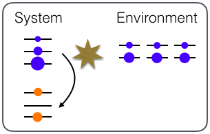
Figure 2: An example of an ’X machine’ setup. These machines use thermal resources (a three-spin microbath in this case) to execute a non-thermodynamic task such as the depletion of the second level in the qutrit system. Since the goal of this type of machines is not to manipulate average energy or entropy, the second law does not set a performance bound for such machines.

On top of their potential practical value, X machines present us with fantastic and exciting thermodynamic challenges. The minimization of $\left\langle\mathcal{A}_{target}\right\rangle$ may be completely unrelated to changes in the average energy or in the entropy. Thus, even in cases where the CI holds for X machines, it does not provide a performance bounds. For example, how well can these machines perform as a function of the initial temperature of the environment and its size? To understand this, it is vital to find additional CI-like inequalities that will relate changes in $\left\langle\mathcal{A}_{target}\right\rangle$ (output), to changes in the microbath (resources). In analogy to reversible processes in conventional machines, it will be very appealing to find bounds that can be saturated by known protocols.

VI.4 Detecting heat leaks and lazy Maxwell’s demons

The CI has a clear regime of validity. If, for some reason, we find that in our setup the CI does not hold, we can conclude that the process in this setup is outside the regime of validity of the CI. The information on being outside the regime of validity can be used to deduce some conclusions on the cause of the anomaly. For example, in a Maxwell demon setup, if we see heat flowing from the cold bath to the hot bath (CI violation) without applying work, we can deduce the existence of a Maxwell demon even if we do not observe the demon directly, only the outcome of its operation. Similarly, in thermodynamic setups in superconducting circuits, a violation of the CI may indicate that the intrinsic thermalization to the background temperature cannot be ignored. Thus, CI violation can provide information on the setup and on the processes that take place.

Next, we ask how far it is possible to push this notion of detection using the violation of thermodynamic inequalities. Perhaps the simplest scenario to consider is the “lazy Maxwell demon” (Uzdin and Rahav, 2018). The setup is initialized with cold molecules in one chamber and hot molecules in another. A Maxwell demon that controls a trap door between the chambers, measures the speed of the incoming molecules on both sides, and according to the results, it decides whether to open or close the door. If the demon performs properly, it can make the cold bath colder and the hot bath hotter. This violation of the CI occurs since feedback operations (the demon’s action) are outside the regime of validity of the CI (unless the feedback mechanism is included in the setup (Leff and Rex, 2014)).

Consider the case where the demon is lazy, and it often dozes off while the trap door is open. In these cases, the average energy (heat) flows naturally from the hot bath to the cold bath. If the fraction of the time when the demon is awake is too small, the cold bath will get warmer, and the hot bath will get colder. Since in this case the CI is not violated, the demon cannot be detected using the CI. We ask if there are other thermodynamic inequalities that can detect the presence of feedback even when the first moment of the energies change consistently with the CI. In (Uzdin and Rahav, 2018) it was shown for a specific example that global passivity inequalities (Uzdin and Rahav, 2018) can detect lazy demons that the CI cannot detect. If, however, the feedback is too weak (a very lazy demon), even the global passivity inequalities in (Uzdin and Rahav, 2018) may not be able to detect it.

Although the findings in (Uzdin and Rahav, 2018) show that this kind of improved thermodynamic demon detection can exist, a big question still remains: can any feedback operation, even a very subtle one, be detected by some thermodynamic constraints on observables such as the CI? Most likely, the resolution of this question will lead to a more comprehensive thermodynamic framework.

VI.5 Deviation from the standard energy-information paradigm

In this chapter, an emphasis has been put on the energy-information structure of the CI. However, in (Goold et al., 2015) a fluctuation theorem has been used to derive an elegant relation between average heat and a new type of measure $\mathcal{B}_{Q}$ that replaces the entropy change of the system. The $B_{Q}$ measure is defined as

$$B_{Q}=-\text{ln}tr(M\rho_{0}^{s}),$$ (70)

where

$$M=tr_{E}[U(\rho^{env}\otimes I^{sys})U^{\dagger}],$$ (71)

and $U$ stands for the global evolution operator. $M$ describes how a system identity state ($I^{sys}/tr[I^{sys}]$, super hot state), evolves under the operator $U$. The relation to heat found in (Goold et al., 2015) is

$$\beta q\geq B_{Q}.$$ (72)

It is both interesting and important to understand the advantages and disadvantages of $B_{Q}$ (and similar measures) with respect to the CI.

As mentioned in Sec. III.4 one of the deficiencies of the CI is its trivial prediction for extremely cold microbaths. It simply predicts that energy in this super cold bath will increase. This problem has been elegantly addressed for an harmonic oscillator system using a phase space approach (Santos et al., 2017). For an initial Gaussian state, the authors find a CI-like relation between the purity and the heat. In the CI-like expression in (Santos et al., 2017) the diverging $\beta$ factor is replaced by an expression that does not diverge as $\beta\to\infty$.

Another interesting deviation from the standard energy-information employs catalysts and many copies of the same setup (Bera et al., 2017). Using the theorem described in (Bera et al., 2017) (see also (Sparaciari et al., 2017)), it is possible to employ a global unitary and an external catalyst to change a given initial density matrix $\rho_{0}$ to any isentropic state $\rho_{f}$ such that $S(\rho_{f})=S(\rho_{0})$. Thus, it is possible to transform the initial state to a thermal state $\rho_{\beta_{eff}}$, whose temperature $1/\beta_{eff}$ is chosen to satisfy $S(\rho_{0})=S(\rho_{\beta_{eff}})$. Now, all initial non-equilibrium scenarios can be treated as if they are initially thermal with some effective temperature. For example, if there is a non-thermal reservoir one can write a Clausius inequality for it with $1/\beta_{eff}$ as its initial temperature.

It is interesting to pursue these approaches and to find new approaches that can overcome the deficiencies of the CI.

VI.6 Fluctuation theorems and CI extensions

As mentioned in Sec. III.3, in their regime of validity, fluctuation theorems (FT) yield stronger statements than the CI, and they can reduce to the CI by using some mathematical inequalities such as the Jensen inequality. As described in Sec. IV.5 (Ref. (Uzdin and Rahav, 2018)) and in Sec. VI.2 (Ref. (Uzdin, 2017)) non-trivial extension of the CI can be derived. These extensions provide inequalities on new observables (e.g., higher order energy moments), and can extend the regime of validity of the CI (e.g., to initial system-environment correlation).

It is fascinating to investigate if some of these new CI extensions can be obtained from fluctuation theorems.

References

- Landauer (1961) R. Landauer, IBM journal of research and development 5, 183 (1961).
- Reeb and Wolf (2014) D. Reeb and M. M. Wolf, New Journal of Physics 16, 103011 (2014).
- Brandão et al. (2015) F. Brandão, M. Horodecki, N. Ng, J. Oppenheim, and S. Wehner, Proceedings of the National Academy of Sciences 112, 3275 (2015).
- Horodecki and Oppenheim (2013) M. Horodecki and J. Oppenheim, Nature communications 4, 2059 (2013).
- Lostaglio et al. (2015) M. Lostaglio, D. Jennings, and T. Rudolph, Nature communications 6, 6383 (2015).
- Uzdin (2017) R. Uzdin, Physical Review E 96, 032128 (2017).
- Peres (2006) A. Peres, Quantum theory: concepts and methods, Vol. 57 (Springer Science & Business Media, 2006).
- Esposito and Van den Broeck (2011) M. Esposito and C. Van den Broeck, EPL (Europhysics Letters) 95, 40004 (2011).
- Sagawa (2012) T. Sagawa, Lectures on Quantum Computing, Thermodynamics and Statistical Physics 8, 127 (2012).
- Strasberg et al. (2017) P. Strasberg, G. Schaller, T. Brandes, and M. Esposito, Physical Review X 7, 021003 (2017).
- Lostaglio et al. (2017) M. Lostaglio, D. Jennings, and T. Rudolph, New Journal of Physics 19, 043008 (2017).
- Guryanova et al. (2016) Y. Guryanova, S. Popescu, A. J. Short, R. Silva, and P. Skrzypczyk, Nat Commun 7, 12049 (2016).
- Halpern et al. (2016) N. Y. Halpern, P. Faist, J. Oppenheim, and A. Winter, Nature Communications 7, 12051 (2016).
- Jarzynski (1999) C. Jarzynski, Journal of Statistical Physics 96, 415 (1999).
- Deffner and Jarzynski (2013) S. Deffner and C. Jarzynski, Physical Review X 3, 041003 (2013).
- Deffner and Lutz (2010) S. Deffner and E. Lutz, Physical review letters 105, 170402 (2010).
- Nielsen and Chuang (2002) M. A. Nielsen and I. Chuang, “Quantum computation and quantum information,” (2002).
- Marshall et al. (1979) A. W. Marshall, I. Olkin, and B. C. Arnold, Inequalities: theory of majorization and its applications, Vol. 143 (Springer, 1979).
- P. Oscar Boykin, Tal Mor, Vwani Roychowdhury, Farrokh Vatan, and Rutger Vrijen (2002) P. Oscar Boykin, Tal Mor, Vwani Roychowdhury, Farrokh Vatan, and Rutger Vrijen, Proc. Nat. Acad. Sci. 99, 3388 (2002).
- Jarzynski (2011) C. Jarzynski, Annu. Rev. Condens. Matter Phys. 2, 329 (2011).
- Speck and Seifert (2007) T. Speck and U. Seifert, Journal of Statistical Mechanics: Theory and Experiment 2007, L09002 (2007).
- Harris and Schütz (2007) R. Harris and G. Schütz, Journal of Statistical Mechanics: Theory and Experiment 2007, P07020 (2007).
- Campisi et al. (2015) M. Campisi, J. Pekola, and R. Fazio, New Journal of Physics 17, 035012 (2015).
- Jarzynski (1997) C. Jarzynski, Physical Review Letters 78, 2690 (1997).
- Micadei et al. (2017) K. Micadei, J. P. Peterson, A. M. Souza, R. S. Sarthour, I. S. Oliveira, G. T. Landi, T. B. Batalhão, R. M. Serra, and E. Lutz, arXiv preprint arXiv:1711.03323 (2017).
- Roßnagel et al. (2014) J. Roßnagel, O. Abah, F. Schmidt-Kaler, K. Singer, and E. Lutz, Physical review letters 112, 030602 (2014).
- Manzano et al. (2015) G. Manzano, F. Galve, R. Zambrini, and J. M. Parrondo, arXiv preprint arXiv:1512.07881 (2015).
- Maslennikov et al. (2017) G. Maslennikov, S. Ding, R. Hablutzel, J. Gan, A. Roulet, S. Nimmrichter, J. Dai, V. Scarani, and D. Matsukevich, arXiv preprint arXiv:1702.08672 (2017).
- Niedenzu et al. (2018) W. Niedenzu, V. Mukherjee, A. Ghosh, A. G. Kofman, and G. Kurizki, Nature communications 9, 165 (2018).
- A. E. Allahverdyan, R. Balian, and Th. M. Nieuwenhuizen (2004) A. E. Allahverdyan, R. Balian, and Th. M. Nieuwenhuizen, Euro. Phys. Lett. 67, 565 (2004).
- Perarnau-Llobet et al. (2017) M. Perarnau-Llobet, E. Bäumer, K. V. Hovhannisyan, M. Huber, and A. Acin, Physical review letters 118, 070601 (2017).
- Bera et al. (2017) M. N. Bera, A. Riera, M. Lewenstein, and A. Winter, arXiv preprint arXiv:1707.01750 (2017).
- Streltsov et al. (2017) A. Streltsov, G. Adesso, and M. B. Plenio, Reviews of Modern Physics 89, 041003 (2017).
- Uzdin and Rahav (2018) R. Uzdin and S. Rahav, Phys. Rev. X, In press, arXiv 1805.00220 (2018).
- Kammerlander and Anders (2016) P. Kammerlander and J. Anders, Scientific Reports 6, 22174 (2016).
- Still et al. (2012) S. Still, D. A. Sivak, A. J. Bell, and G. E. Crooks, Physical review letters 109, 120604 (2012).
- Pusz and Wornwicz (1978) W. Pusz and S. Wornwicz, Commun. Math. Phys. 58, 273 (1978).
- Lenard (1978) A. Lenard, Journal of Statistical Physics 19, 575 (1978).
- Perarnau-Llobet et al. (2015a) M. Perarnau-Llobet, K. V. Hovhannisyan, M. Huber, P. Skrzypczyk, J. Tura, and A. Acín, Physical Review E 92, 042147 (2015a).
- Perarnau-Llobet et al. (2015b) M. Perarnau-Llobet, K. V. Hovhannisyan, M. Huber, P. Skrzypczyk, N. Brunner, and A. Acín, Phys. Rev. X 5, 041011 (2015b).
- Amikam Levy and Ronnie Kosloff (2012) Amikam Levy and Ronnie Kosloff, Phys. Rev. Lett. 108, 070604 (2012).
- Kirkwood (1935) J. G. Kirkwood, The Journal of Chemical Physics 3, 300 (1935).
- Jarzynski (2017) C. Jarzynski, Physical Review X 7, 011008 (2017).
- Seifert (2016) U. Seifert, Physical review letters 116, 020601 (2016).
- Miller and Anders (2017) H. J. D. Miller and J. Anders, Phys. Rev. E 95, 062123 (2017).
- Anders and Giovannetti (2013) J. Anders and V. Giovannetti, New Journal of Physics 15, 033022 (2013).
- (47) R. Uzdin, In preperation .
- Brask et al. (2015) J. B. Brask, G. Haack, N. Brunner, and M. Huber, New Journal of Physics 17, 113029 (2015).
- Tacchino et al. (2018) F. Tacchino, A. Auffèves, M. Santos, and D. Gerace, Physical review letters 120, 063604 (2018).
- Leff and Rex (2014) H. S. Leff and A. F. Rex, Maxwell’s demon: entropy, information, computing (Princeton University Press, 2014).
- Goold et al. (2015) J. Goold, M. Paternostro, and K. Modi, Physical review letters 114, 060602 (2015).
- Santos et al. (2017) J. P. Santos, G. T. Landi, and M. Paternostro, Physical review letters 118, 220601 (2017).
- Sparaciari et al. (2017) C. Sparaciari, D. Jennings, and J. Oppenheim, Nature communications 8, 1895 (2017).