Local-Global Convergence,
an analytic and structural approach

Abstract.

Based on methods of structural convergence we provide a unifying view of local-global convergence, fitting to model theory and analysis. The general approach outlined here provides a possibility to extend the theory of local-global convergence to graphs with unbounded degrees. As an application, we extend previous results on continuous clustering of local convergent sequences and prove the existence of modeling quasi-limits for local-global convergent sequences of nowhere dense graphs.

The true logic of the world is in the calculus of probabilities

1. Introduction

The study of graph limits recently gained a strong interest, motivated both by the study of large networks and the emerging studies of real evolving networks. The different notions of graph limit (left convergence [7, 8, 9, 10, 19], local convergence [5]), and the basic notions of graph similarity on which they are based, opens a vast panorama. These frameworks have in common to be built on statistics of locally defined motives when the vertices of the graphs in the sequence are sampled uniformly and independently. A unified framework for the study of convergence of structures has been introduced by the authors in [20].

In this setting the notion of convergence is, in essence, model theoretic, and relies on the the following notions:

For a $\sigma$-structure $\mathbf{A}$ and a first-order formula $\phi$ (in the language of $\sigma$, with free variables $x_{1},\dots,x_{p}$), we denote by $\phi(\mathbf{A})$ the satisfying set of $\phi$ in $\mathbf{A}$:

$$\phi(\mathbf{A})=\{(v_{1},\dots,v_{p})\in A^{p}:\ \mathbf{A}\models\phi(v_{1},\dots,v_{p})\},$$

and we define the Stone pairing of $\phi$ and $\mathbf{A}$ as the probability

$$\langle\phi,\mathbf{A}\rangle=\frac{|\phi(\mathbf{A})|}{|A|^{p}}$$

that $\mathbf{A}$ satisfies $\phi$ for a (uniform independent) random interpretation of the random variables.

A sequence $\boldsymbol{\mathsf{A}}=(\mathbf{A}_{n})_{n\in\mathbb{N}}$ of finite $\sigma$-structures is ${\rm FO}$-convergent if the sequence $\langle\phi,\boldsymbol{\mathsf{A}}\rangle=(\langle\phi,\mathbf{A}_{n}\rangle)_{n\in\mathbb{N}}$ converges for every first-order formula $\phi$. One similarly defines a weakened notion of $X$-convergence (for a fragment $X$ of first-order logic) by restricting the range of the test formulas $\phi$ to $X$. In particular, for a sequence of graphs with growing orders, the ${\rm QF}$-convergence (that is of convergence driven by the fragment ${\rm QF}$ of quantifier-free formulas) is equivalent to left convergence, and the ${\rm FO}^{\rm local}$-convergence (that is of convergence driven by the fragment ${\rm FO}^{\rm local}$ of the so-called local formulas) is equivalent to local convergence when restricting to sequences of graphs with bounded degrees [20]. The study of $X$-convergence of structures and the related problems is called shortly “structural limits”. It extends all previously considered types of non-geometric convergence of combinatorial structures (two above and also, e.g. permutations) to general relational structures. A survey of structural limits can be found in [22, 21].

In order to strengthen the notion of local convergence of sequences of connected bounded degree graphs, the notion of local-global convergence has been introduced by Hatami and Lovász [12], based on the framework introduced in [6]. The orignal definition of local-global convergence, which is based on the total variation distance between the distributions of colored neighborhoods of radius $r$ in the graphs in the sequence, is admittedly quite technical (see Definitions 3.3.1 and 3.4.1). Roughly speaking, the strengthening of local convergence into local-global convergence relates to the extension of the considered properties from first-order logic to existential monadic second order logic.

In this paper we introduce the notion of lift-Hausdorff convergence, which is defined generally for graphs and relational structures, based on a simple subsequence completion property (see Definition 3.4.3). The basic notions underlying this definition are the model theoretic notions of lift of a structure (that one can see as an augmentation of a structure by colors, new relations, etc.) and the dual notion of shadow consisting in forgetting all the additional relations of a lift (see Fig. 1). Note that the notions of lift and shadow are close to model theoretic notions of expansion and reduct.

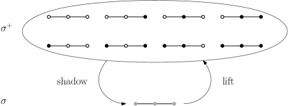
Figure 1. The shadow operation consists in forgetting some of the relations, while the lift operation consists in adding some relations in all possible ways.

A lift/shadow pair is determined by the data of two signatures $\sigma\subset\sigma^{+}$, the signature of the shadows and the signature of the lifts. Given a lift/shadow pair, the corresponding notion of lift-Hausdorff convergence is (roughly) defined as follows: A sequence $\boldsymbol{\mathsf{A}}=(\mathbf{A}_{n})_{n\in\mathbb{N}}$ is lift-Hausdorff convergent if, for every convergent subsequence $\boldsymbol{\mathsf{A}}_{f}^{+}=(\mathbf{A}_{f(n)}^{+})_{n\in\mathbb{N}}$ of lifts there exists a (full) convergent sequence $\boldsymbol{\mathsf{A^{*}}}$ of lifts extending $\boldsymbol{\mathsf{A}}_{f}^{+}$ . (In this definition, the condition that $\boldsymbol{\mathsf{A}}_{f}$ is a subsequence of lifts means that $\mathbf{A}_{f(n)}^{+}$ is a lift of $\mathbf{A}_{f(n)}$ and $f:\mathbb{N}\rightarrow\mathbb{N}$ is an increasing function defining a subsequence of indices; the condition that $\boldsymbol{\mathsf{A}}^{*}$ extends $\boldsymbol{\mathsf{A}}_{f}^{+}$ means that $\mathbf{A}_{f(n)}^{*}=\mathbf{A}_{f(n)}^{+}$ for every integer $n$.)

We prove that this notion indeed extends the usual notion of local-global convergence in the case of monadic lifts and gives a characterization of lift-Hausdorff convergent sequences as Cauchy sequences for an appropriate metric (Theorem 3.3.2). Note that the case of monadic lifts can be interpreted by means of first-order formulas with set parameters.

We give a basic representation theorem for corresponding limits, which is based on the representation theorem for structural limits [20]: every limit of a lift-Hausdorff convergent sequence maybe represented by non-empty closed subset of the space of probability measures on some Stone space (Theorem 3.3.3). In Section 4.2 we discuss the possible notion of a limit object for lift-Hausdorff convergent sequences. Two possible notions can be considered:

• a strong notion of limit $\mathbf{L}$ for a sequence $\boldsymbol{\mathsf{A}}$, such that for every convergent sequence $\boldsymbol{\mathsf{A}}^{+}$ of lifts there exists an admissible lift $\mathbf{L}^{+}$ of $\mathbf{L}$ that is the limit of $\boldsymbol{\mathsf{A}}^{+}$ and, conversely, for every admissible lift $\mathbf{L}^{+}$ of $\mathbf{L}$ there exists a convergent sequence $\boldsymbol{\mathsf{A}}^{+}$ of lifts with limit $\mathbf{L}^{+}$;

• a weaker notion of limit $\mathbf{L}$ (in the spirit of the representation of local-global limits by graphings [12]) where we ask that for every $\epsilon>0$ and every convergent sequence $\boldsymbol{\mathsf{A}}^{+}$ of lifts there exists an admissible lift $\mathbf{L}^{+}$ of $\mathbf{L}$ such that for every formula $\phi$ we have

  (1) $$\bigl{|}\langle\phi,\mathbf{L}^{+}\rangle-\lim_{n\rightarrow\infty}\langle\phi,\mathbf{A}_{n}^{+}\rangle\bigr{|}<c_{\phi}\epsilon$$

  (where $c_{\epsilon}$ is a positive constant depending only on $\phi$) and, conversely, for every admissible lift $\mathbf{L}^{+}$ of $\mathbf{L}$ there exists a convergent sequence $\boldsymbol{\mathsf{A}}^{+}$ of lifts such that (1) holds.

In these definitions, an essential difficulty lies in the definition of admissible lifts. In the case of local-global convergent sequences of bounded degree graphs with a graphing limit, the notion of admissible lift corresponds to Borel colorings. In a more general setting, an admissible lift of a modeling should (at least) be a modeling itself. However, Borel colorings of a fixed graphing does not induce a closed subset of unimodular probability measures, as noticed in [12] and, more generally, probability measures associated to modeling lifts of a fixed modeling does not form a closed subset, what is problematic for the stronger notion of limit.

When considering the weaker (standard) definition of a limit, the reverse direction appears to be quite difficult to handle in general. Indeed, in the bounded degree case, the $r$-neighborhood of a set with measure at most $\epsilon$ has measure a most $d^{r}\epsilon$, what allows to easily approximates Borel colorings using a countable base. However such a property does not hold in the general unbounded degree case.

For this reason, we only consider one direction in the definition of limit: a quasi-limit $\boldsymbol{\mathsf{A}}$ is a modeling such that for every $\epsilon>0$, every formula $\phi$ and every convergent sequence $\boldsymbol{\mathsf{A}}^{+}$ of lifts there exists a modeling lift $\mathbf{L}^{+}$ of $\mathbf{L}$ such that (1) holds. In this setting, we prove that modelings (introduced in [25]) are not only limit objects for FO-convergent nowhere dense sequences (as proved in [26]) but also quasi-limits for (monadic) lift-Hausdorff convergent nowhere dense sequences (see Theorem 4.2.4).

This paper is organized as follows:

1. 1 Introduction
2. 2 Preliminaries
   1. 2.1 Relational Structures and First-Order Logic
   2. 2.2 Functional Analysis
   3. 2.3 Sequences
   4. 2.4 Basics of Structural Convergence
   5. 2.5 The Representation Theorem for Structural Limits
3. 3 From interpretation to lift convergence
   1. 3.1 A Categorical Approach to Interpretations
   2. 3.2 Metric properties of interpretations
   3. 3.3 Lift-Hausdorff convergence
   4. 3.4 Local Global Convergence
4. 4 Applications
   1. 4.1 Clustering
   2. 4.2 Local Global Quasi-Limits

Let us end this introduction by few remarks. The lifts involved in our local-global structural convergence are all monadic (and can be seen as coloring of vertices). It follows that the expressive power of such lifts is restricted to embeddings and classes which are hereditary. If we would consider more general lifts, such as coloring of the edges then we could represent monomorphisms (not induced substructures) which in turn leads to monotone classes. Monotone classes of graphs which have modeling limits (of which graphing limits are a particular case) were characterized in [26] and coincides with nowhere dense classes (of graphs). This also coincides (in the case of monotone classes of graphs) with the notion of NIP and stable classes [1] (See also [23]). For hereditary classes the structure theory and the existence of modeling limits is more complicated (see [22]) and local-global convergence seems to provide a useful framework.

2. Preliminaries

2.1. Relational Structures and First-Order Logic

A signature $\sigma$ is a set of relation symbols with associated arities. In this paper we will consider countable signatures. A $\sigma$-structure $\mathbf{A}$ is defined by its domain $A$, which is a set, and by interpreting each relation symbol $R\in\sigma$ of arity $k$ as a subset of $A^{k}$. We denote by ${\rm Rel}(\sigma)$ the set of all finite $\sigma$-structures and by $\mathscr{R}\rm{el}(\sigma)$ the class of all $\sigma$-structures.

A first-order formula $\phi$ in the language of $\sigma$-structures is a formula constructed using disjunction, conjunction, negation and quantification over elements, using the relations in $\sigma$ and the equality symbol. A variable used in a formula $\phi$ is free if it is not bound by a quantifier. We always assume that free variables are named $x_{1},\dots,x_{n},\dots$ and we consider formulas obtained by renaming the free variables as distinct. For instance, $x_{1}=x_{2}$ and $x_{2}=x_{3}$ are distinct formulas. We also consider two constants, $0$ and $1$ to denote the false and true statements. We denote by ${\rm FO}(\sigma)$ the (countable) set of all first-order formulas in the language of $\sigma$-structures. The conjunction and disjunction of formulas $\phi$ and $\psi$ are denoted by $\phi\wedge\psi$ and $\phi\vee\psi$, and the negation of $\phi$ is denoted by $\neg\phi$. We say that two formulas $\phi$ and $\psi$ are logically equivalent, which we denote by $\phi\iff\psi$, if one can infer one from the other (i.e. $\phi\vdash\psi$ and $\psi\vdash\phi$). Note that in first-order logic the notions of syntactic and semantic equivalence coincides. In this context we denote by $[\phi]$ the equivalence class of $\phi$ with respect to logical equivalence. It is easily checked that $\mathcal{B}_{\sigma}={\rm FO}(\sigma)/\!\!\!\!\iff$ is a countable Boolean algebra with minimum $0$ and maximum $1$, which is called the Lindenbaum-Tarki algebra of ${\rm FO}(\sigma)$.

In this paper we consider special fragments of first-order logic (see Table 1).

sshv Symbol	Fragment
vhv ${\rm FO}(\sigma)$ or ${\rm FO}$	All first order formulas
${\rm FO}_{p}(\sigma)$ or ${\rm FO}_{p}$	All first order formulas with free variables within $\{x_{1},\dots,x_{p}\}$
${\rm FO}_{0}(\sigma)$ or ${\rm FO}_{0}$	Sentences
${\rm FO}^{\rm local}(\sigma)$ or ${\rm FO}^{\rm local}$	Local formulas
${\rm FO}_{p}^{\rm local}(\sigma)$ or ${\rm FO}_{p}^{\rm local}$	Local formulas with free variables within $\{x_{1},\dots,x_{p}\}$
${\rm QF}(\sigma)$ or ${\rm QF}$	Quantifier free formulas
vhss

Table 1. Principal fragments of first-order logic considered in this paper.

The Lindenbaum-Tarski algebra of a fragment $X\subseteq{\rm FO}(\sigma)$ will be denoted by $\mathcal{B}_{\sigma}^{X}$. For instance, $\mathcal{B}_{\sigma}^{\rm QF}={\rm QF}(\sigma)/\!\!\!\!\iff$.

2.2. Functional Analysis

Basic facts from Functional Analysis, which will be used in this paper, are recalled now.

A standard Borel space is a Borel space associated to a Polish space, i.e. a measurable space $(X,\Sigma)$ such that there exists a metric on $X$ making it a separable complete metric space with $\Sigma$ as its Borel $\sigma$-algebra. Typical examples of standard Borel spaces are $\mathbb{R}$ and the Cantor space. Note that according to Maharam’s theorem, all uncountable standard Borel spaces are (Borel) isomorphic. (The authors cannot resist the temptation to mention Balcar’s award-winning work [4] in this context.)

In this paper, we shall mainly consider compact separable metric spaces. Note that if $(M,{\rm d})$ is a compact separable metric space, then linear functionals on the space of real continuous functions on $M$ can be represented, thanks to Riesz-Markov-Kakutani representation theorem, by Borel measures on $M$. We denote by $P(M)$ the space of all probability measures on $M$. A sequence of probability measures $(\mu_{n})_{n\in\mathbb{N}}$ is weakly convergent if $\int f\,{\rm d}\mu_{n}$ converges for every (real-valued) continuous function $f$. Weak convergence defines the weak topology of $P(M)$, and (as we assumed that $(M,d)$ is a compact separable metric space) this space is compact, separable, and metrizable by the Lévy-Prokhorov metric (based on the metric ${\rm d}$):

$${\rm d}^{\rm LP}(\mu_{1},\mu_{2})=\inf\Bigl{\{}\epsilon>0\mid\mu_{1}(A)\leq\mu_{2}(A^{\epsilon})+\epsilon\text{ and }\mu_{2}(A)\leq\mu_{1}(A^{\epsilon})+\epsilon\text{ for all Borel }A\Bigr{\}},$$

where $A^{\epsilon}=\{x\in M\mid(\exists y\in M)\ {\rm d}(x,y)<\epsilon\}$.

The Hausdorff metric is defined on the space of nonempty closed bounded subsets of a metric space. Consider a compact metric space $(M,{\rm d})$, and let $\mathscr{C}_{M}$ be the space of non-empty closed subsets of $M$ endowed with the Hausdorff metric defined by

$${\rm d}^{\rm H}(X,Y)=\max\bigl{(}\adjustlimits{\max}_{x\in X}{\min}_{y\in Y}{\rm d}(x,y),\max_{y\in Y}\min_{x\in X}{\rm d}(x,y)\bigr{)}.$$

One of the most important properties of Hausdorff metric is that the space of non-empty closed subsets of a compact set is also compact (see [13], and [27] for an independent proof). Hence the space $(\mathscr{C}_{M},{\rm d}^{\rm H})$ is compact.

We can use the inverse function of a surjective continuous function from a compact metric space $(M,{\rm d})$ to a (thus compact) Hausdorff space $T$ to isometrically embed the space $\mathscr{C}_{T}$ (of non-empty closed subsets of $T$) into $(\mathscr{C}_{M},{\rm d}^{\rm H})$. Then, using the natural injection $\iota:T\rightarrow\mathscr{C}_{T}$ (defined by $\iota(x)=\{x\}$) we pull back the Hausdorff distance on $\mathscr{C}_{M}$ into $T$:

$${\rm d}_{T}(x,y)={\rm d}^{\rm H}(f^{-1}(x),f^{-1}(y)).$$

The situation is summarized in the following diagram.

In this diagram $f^{-1}$ denotes the mapping from $T$ to $\mathscr{C}_{M}$ and $\hat{f}^{-1}$ the corresponding mapping from $\mathscr{C}_{T}$ to $\mathscr{C}_{M}$ defined by $\hat{f}^{-1}(X)=\{y\mid f(y)\in X\}$. Also remark that the metric ${\rm d}_{T}$ defined on $T$ is usually not compatible with the original topology of $T$.

For the topology defined by the metric ${\rm d}_{T}$, one can define the compactification of $T$, which may be identified with the closure of the image of $T$ (by $f^{-1}\circ\iota$) in $\mathscr{C}_{M}$.

We shall make use of the following folklore result, which we prove here for completeness.

Lemma 2.2.1.

Let $X,Y$ be compact standard Borel spaces and let $f:X\rightarrow Y$ be continuous. Let $P(X)$ and $P(Y)$ denote the metric space of probability measures on $X$ and $Y$ (with Lévy-Prokhorov metric).

Then the pushforward by $f$, that is the mapping $f_{*}:P(X)\rightarrow P(Y)$ defined by $f_{*}(\mu)=\mu\circ f^{-1}$, is continuous.

Proof.

Assume $\mu_{n}\Rightarrow\mu$ is a weakly convergent sequence of measures in $P(X)$. Then for every continuous function $g:Y\rightarrow\mathbb{R}$ it holds

$$\int_{Y}g(y)\,{\rm d}f_{*}(\mu)(y) =\int_{X}g\circ f(x)\,{\rm d}\mu(x)$$

$$=\lim_{n\rightarrow\infty}\int_{X}g\circ f(x)\,{\rm d}\mu_{n}(x)$$

$$=\lim_{n\rightarrow\infty}\int_{Y}g(y)\,{\rm d}f_{*}(\mu_{n})(y)$$

Hence $f_{*}(\mu_{n})\Rightarrow f_{*}(\mu)$. ∎

2.3. Sequences

In this paper we denoted sequences by sans serif letters. In particular, we denote by $\boldsymbol{\mathsf{A}}$ a sequence of structures $\boldsymbol{\mathsf{A}}=(\mathbf{A}_{n})_{n\in\mathbb{N}}$, and by $\mathsf{X}=(X_{n})_{n\in\mathbb{N}}$ a sequence of sets $X_{n}$, where $X_{n}$ is a subset of the domain $A_{n}$ of $\mathbf{A}_{n}$.

Subsequences will by denoted by $\boldsymbol{\mathsf{A}}_{f}$ and $\mathsf{X}_{f}$, where $f$ is meant to be a strictly increasing function $f:\mathbb{N}\rightarrow\mathbb{N}$, and represent the sequences $(\mathbf{A}_{f(n)})_{n\in\mathbb{N}}$ and $(X_{f(n)})_{n\in\mathbb{N}}$. Note that $(\boldsymbol{\mathsf{A}}_{f})_{g}=\boldsymbol{\mathsf{A}}_{g\circ f}$.

In order to simplify the notations, we extend binary relations and standard constructions to sequences by applying them component-wise. For instance $\mathsf{X}\subseteq\mathsf{Y}$ means $(\forall n\in\mathbb{N})\ X_{n}\subseteq Y_{n}$, $\mathsf{X}\cap\mathsf{Y}$ represents the sequence $(X_{n}\cap Y_{n})_{n\in\mathbb{N}}$, and if $f:{\rm Rel}(\sigma)\rightarrow\mathbb{R}$ is a mapping then $f(\boldsymbol{\mathsf{A}})$ represents the sequence $(f(\mathbf{A}_{n}))_{n\in\mathbb{N}}$.

We find these notations extremely helpful for our purposes.

2.4. Basics of Structural Convergence

Let $\sigma$ be a countable signature, let $X$ be a fragment of ${\rm FO}(\sigma)$. For $\phi\in X$ with free variables within $x_{1},\dots,x_{p}$ and $\mathbf{A}$, we denote by $\langle\phi,\mathbf{A}\rangle$ the probability that $\phi$ is satisfied in $\mathbf{A}$ for a random assignment of elements of $A$ to the free variables of $\phi$ (for an independent and uniform random choice of the assigned elements), that is:

$$\langle\phi,\mathbf{A}\rangle=\frac{\bigl{|}\bigr{\{}\overline{v}\in A^{p}\mid\mathbf{A}\models\phi(\overline{v})\bigr{\}}\bigr{|}}{|A|^{p}}.$$

(Note that the presence of unused free variables does not change the value in the next equation.) In the special case where $\phi$ is a sentence, we get

$$\langle\phi,\mathbf{A}\rangle=\begin{cases}1&\text{if }\mathbf{A}\models\phi,\\ 0&\text{otherwise}\end{cases}$$

Two $\sigma$-structures $\mathbf{A}$ and $\mathbf{B}$ are $X$-equivalent, what we denote by $\mathbf{A}\equiv_{X}\mathbf{B}$, if we have $\langle\phi,\mathbf{A}\rangle=\langle\phi,\mathbf{B}\rangle$ for every $\phi\in X$.

Example 2.4.1.

Let ${\rm QF}^{-}$ be the fragment of quantifier-free formulas that do not use equality.

The case of ${\rm FO}^{\rm local}_{1}$-equivalence is settled by the next proposition.

Proposition 2.4.2.

For any two finite $\sigma$-structures $\mathbf{A}$ and $\mathbf{B}$ we have that $\mathbf{A}\equiv_{{\rm FO}_{1}^{\rm local}}\mathbf{B}$ if and only if there exists a finite $\sigma$-structure $\mathbf{C}$ and two positive integers $a$ and $b$ such that $\mathbf{A}$ is isomorphic to $a$ copies of $\mathbf{C}$ and $\mathbf{B}$ is isomorphic to $b$ copies of $\mathbf{C}$.

Proof.

Let $\mathbf{F}_{1},\dots,\mathbf{F}_{n},\dots$ be an enumeration of the finite $\sigma$-structures (up to isomorphism), and let $\varphi_{i}(x)$ be a local formula expressing that the connected component of $x$ is isomorphic to $\mathbf{F}_{i}$ (i.e. that the ball of radius $|F_{i}|+1$ around $x$ is isomorphic to $F_{i}$). Then $\langle\varphi_{i},\mathbf{A}\rangle$ is equal to the product of $|\mathbf{F}_{i}|/|\mathbf{A}|$ by the number of connected components of $\mathbf{A}$ isomorphic to $\mathbf{F}_{i}$. Thus there exists a positive integer $q$ and non-negative integers $p_{1},\dots,p_{n},\dots$ such that $\langle\varphi_{i},\mathbf{A}\rangle=p_{i}/q$ and the set of all positive $p_{i}$ values is setwise coprime. Then if $\mathbf{C}$ consists in thus union (over $i$) of $p_{i}$ copies of $\mathbf{F}_{i}$, it is immediate that $\mathbf{A}$ and $\mathbf{B}$ consists in a positive number of copies of $\mathbf{C}$. ∎

A sequence $\boldsymbol{\mathsf{A}}$ of $\sigma$-structures is $X$-convergent if $\langle\phi,\boldsymbol{\mathsf{A}}\rangle=(\langle\phi,\mathbf{A}_{n}\rangle)_{n\in\mathbb{N}}$ converges for each $\phi\in X$. This provides a unifying to left and local convergence, as mentioned in the introduction: left convergence coincides with ${\rm QF}^{-}$-convergence and local convergence with ${\rm FO}^{\rm local}$-convergence (when restricted to graphs with bounded degrees). The term of structural convergence covers the general notions of $X$-convergence.

The basic result of [20], which is going to provide us a guideline for a proper generalization of local-global convergence is the representation theorem for structural limits in terms of probability measures. We adopt [20] to the setting of this paper.

2.5. The Representation Theorem for Structural Limits

For a countable signature $\sigma$ and a fragment $X$ of ${\rm FO}(\sigma)$ we denote by $S_{X}^{\sigma}$ the Stone dual of the Lindenbaum-Tarski $\mathcal{B}_{\sigma}^{X}$ of $X$, which is a compact Polish space. Recall that the points of $\mathcal{B}_{\sigma}^{X}$ are the maximal consistent subsets of $X$ (or equivalently the ultrafilters on $\mathcal{B}_{\sigma}^{X}$). The topology of $S_{X}^{\sigma}$ is generated by the base of the clopen subsets of $S_{X}^{\sigma}$, which are in bijection with the formulas in $X$ by

$$\phi\mapsto K(\phi)=\bigl{\{}t\in S_{X}^{\sigma}\mid\phi\in t\bigr{\}}.$$

In the setting of this paper we work with metric (and, notably, pseudo-metric) spaces. First note that the topology of $S_{X}^{\sigma}$ is metrizable by the several metrics, including the metrics we introduce now.

A chain covering of $X$ is an increasing sequence $\mathfrak{X}=(X_{1},X_{2},\dots)$ of finite sets (i.e. $X_{1}\subset X_{2}\subset\dots\subset X_{n}\subset\dots$) such that every formula in $X$ is logically equivalent to a formula in $\bigcup_{i\geq 1}X_{i}$. The metric $\delta_{\mathfrak{X}}$ induced by $\mathfrak{X}$ on $S_{\sigma}^{X}$ is defined by

• (2) $$\delta_{\mathfrak{X}}(t_{1},t_{2})=\inf\bigl{\{}1/n\mid(t_{1}\vartriangle t_{2})\cap X_{n}=\emptyset\bigr{\}},$$

where $t_{1}\vartriangle t_{2}$ stands for the symmetric difference of the sets $t_{1}$ and $t_{2}$.

First-order limits (shortly ${\rm FO}$-limits) and, more generally, $X$-limits can be uniquely represented by a probability measure $\mu$ on the Stone space $S$ dual to the Lindenbaum-Tarski algebra of the formulas. This can be formulated as follows.

Theorem 2.5.1 ([20]).

Let $\sigma$ be a countable signature, let $X$ be a fragment of ${\rm FO}(\sigma)$ closed under disjonction, conjunction and negation, let $\mathcal{B}^{X}_{\sigma}$ be the Lindenbaum-Tarski algebra of $X$, and let $S^{X}_{\sigma}$ be the Stone dual of $\mathcal{B}^{X}_{\sigma}$.

Then there is a map $T^{X}_{\sigma}$ from the space ${\rm Rel}(\sigma)$ of finite $\sigma$-structures to the space of $P(S_{\sigma}^{X})$ of probability measures on the Stone space $S^{X}_{\sigma}$, such that for every $\mathbf{A}\in{\rm Rel}(\sigma)$ and every $\phi\in X$ we have

(3) $$\langle\phi,\mathbf{A}\rangle=\int_{S_{\sigma}^{X}}\mathbf{1}_{\phi}(t)\,{\rm d}\mu_{\mathbf{A}}(t),$$

where $\mu_{\mathbf{A}}=T^{X}_{\sigma}(\mathbf{A})$ and $\mathbf{1}_{\phi}$ is the indicator function of the clopen subset $K(\phi)$ of $S^{X}_{\sigma}$ dual to the formula $\phi\in X$ in Stone duality, i.e.

$$\mathbf{1}_{\phi}(t)=\begin{cases}1&\text{if }\phi\in t\\ 0&\text{otherwise}.\end{cases}$$

Additionally, if the fragment $X$ includes ${\rm FO}_{0}$ or ${\rm QF}$ then the mapping $T_{\sigma}^{X}$ is one-to-one.

In this setting, a sequence $\boldsymbol{\mathsf{A}}$ of finite $\sigma$-structures is $X$-convergent if and only if the measures $T_{\sigma}^{X}(\mathbf{A}_{n})$ converge weakly to some measure $\mu$. Then for every first-order formula $\phi\in X$ we have

(4) $$\int_{S^{X}_{\sigma}}\mathbf{1}_{\phi}(t)\,{\rm d}\mu(t)=\lim_{n\rightarrow\infty}\int_{S^{X}_{\sigma}}\mathbf{1}_{\phi}(t)\,{\rm d}\mu_{\mathbf{A}_{n}}(t)=\lim_{n\rightarrow\infty}\langle\phi,\mathbf{A}_{n}\rangle,$$

where $\mu_{\mathbf{A}_{n}}=T^{X}_{\sigma}(\mathbf{A}_{n})$.

Assume that a subgroup $\Gamma$ of the group $\mathfrak{S}_{\omega}$ of permutations of $\mathbb{N}$ acts on the first-order formulas in $X$ by permuting the free variables. Then this action induces an action on $S_{\sigma}^{X}$, and the probability measure $T^{X}_{\sigma}(\mathbf{A})$ associated with a finite structure $\mathbf{A}$ is obviously $\Gamma$-invariant, thus so is the weak limit $\mu$ of a sequence $(T^{X}_{\sigma}(\mathbf{A}_{n}))_{n\in\mathbb{N}}$ of probability measures associated with the finite structures of an X-convergent sequence. It follows that the measure $\mu$ appearing in (4) has the property to be $\Gamma$-invariant.

This theorem generalizes the representation of the limit of a left-convergent sequence of graphs by an infinite exchangeable random graph [2, 16] and the representation of the limit of a local-convergent sequence of bounded degree graphs by a unimodular distribution [5]. Figure 2 schematically depicts some of the notions related to the representation theorem.

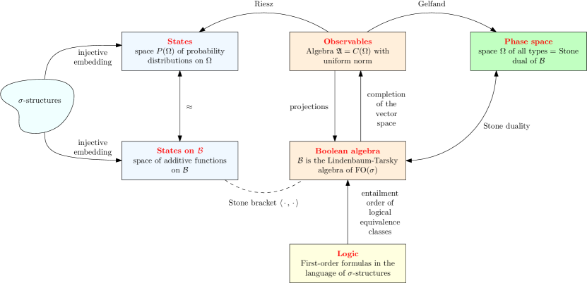
Figure 2. Sketch of the spaces involved in the distributional representation of structural limits of $\sigma$-structures.

The weak topology of $P(S_{\sigma}^{X})$ is metrizable by using the Lévy-Prokhorov metrics based on the metrics $\delta_{\mathfrak{X}}$ (where $\mathfrak{X}$ is a fixed chain covering of $X$). Using the fact that $\delta_{\mathfrak{X}}$ is an ultrametric, we obtain the following more practical expression for the Lévy-Prokhorov metric ${\rm d}_{\mathfrak{X}}^{\rm LP}$ associated to $\delta_{\mathfrak{X}}$:

• (5) $${\rm d}_{\mathfrak{X}}^{\rm LP}(\mu_{1},\mu_{2})=\inf_{n\in\mathbb{N}}\biggl{\{}\max\Bigl{(}1/n,\max_{\phi\in X_{n}}\Bigl{|}\int_{S_{\sigma}^{X}}\mathbf{1}_{\phi}(t)\,{\rm d}(\mu_{1}-\mu_{2})(t)\Bigr{|}\Bigr{)}\biggr{\}}.$$

This metric in turn uniquely defines a pseudometric ${\rm dist}_{\mathfrak{X}}$ on ${\rm Rel}(\sigma)$ such that the mapping $T_{\sigma}^{X}$ induces an isometric embedding of ${\rm Rel}(\sigma)/\!\equiv_{X}$ into $P(S_{\sigma}^{X})$:

$${\rm dist}_{\mathfrak{X}}(\mathbf{A},\mathbf{B})={\rm d}_{\mathfrak{X}}^{\rm LP}(T_{\sigma}^{X}(\mathbf{A}),T_{\sigma}^{X}(\mathbf{B})).$$

Note that we have the following expression for ${\rm dist}_{\mathfrak{X}}$:

• (6) $${\rm dist}_{\mathfrak{X}}(\mathbf{A},\mathbf{B})=\inf_{n\in\mathbb{N}}\Bigl{\{}\max\bigl{(}1/n,\max_{\phi\in X_{n}}|\langle\phi,\mathbf{A}\rangle-\langle\phi,\mathbf{B}\rangle|\bigr{)}\Bigr{\}}.$$

It is easily checked that, as expected, a sequence $\boldsymbol{\mathsf{A}}$ is $X$-convergent if and only if it is Cauchy for ${\rm dist}_{\mathfrak{X}}$.

We denote by $\mathscr{M}^{X}_{\sigma}\subseteq P(S^{X}_{\sigma})$ the space of probability measures on $S^{X}_{\sigma}$ associated to finite $\sigma$-structures:

$$\mathscr{M}^{X}_{\sigma}=\{T^{X}_{\sigma}(\mathbf{A})\mid\mathbf{A}\in{\rm Rel}(\sigma)\}.$$

We denote by $\overline{\mathscr{M}^{X}_{\sigma}}$ the weak closure of $\mathscr{M}^{X}_{\sigma}$ in $P(S^{X}_{\sigma})$ and by $(\overline{{\rm Rel}(\sigma)}^{X},{\rm dist}_{\mathfrak{X}})$ the completion of the pseudometric space $({\rm Rel}(\sigma),{\rm dist}_{\mathfrak{X}})$. Note that $(\overline{{\rm Rel}(\sigma)}^{X},{\rm dist}_{\mathfrak{X}})$ has a dense subspace naturally identified with $({\rm Rel}(\sigma)/\!\!\equiv_{X},{\rm dist}_{\mathfrak{X}})$, and $T_{\sigma}^{X}$ induces an isometric isomorphism of $(\overline{{\rm Rel}(\sigma)}^{X},{\rm dist}_{\mathfrak{X}})$ and $(\overline{\mathscr{M}^{X}_{\sigma}},{\rm d}^{\rm LP}_{\mathfrak{X}})$. Consequently both spaces are separable compact metric spaces.

3. From interpretation to lift convergence

Our basic approach to local-global convergence is by means of lifts of structures, which demands a change of signature. By doing so we still have to preserve some functorial properties and this is done by means of interpretations.

3.1. A Categorical Approach to Interpretations

Interpretations of classes of relational structures in other classes of relational structures are a useful and powerful technique to transfer properties from one class of structures to another (with possibly a different signature).

First, we define interpretations syntactically (in the spirit of [18]), which allows us to organize them as a category. This functorial view will be particularly useful in our setting.

Let $\tau,\sigma$ be countable relationa l signatures. An interpretation $\mathsf{I}$ of $\sigma$-structures in $\tau$-structures is a triple $(\nu,\eta,(\rho_{R})_{R\in\sigma})$, where:

• $\nu(\overline{x})\in{\rm FO}(\tau)$ is a formula defined on $p$ tuples of variables $\overline{x}$;

• $\eta(\overline{x},\overline{y})\in{\rm FO}(\tau)$ is a formula defining an equivalence relation on $p$-tuples (satisfying $\nu$);

• for each relation $R\in\sigma$ of arity $k$, the formula $\rho_{R}(\overline{x}_{1},\dots,\overline{x}_{k})\in{\rm FO}(\tau)$ (with $|\overline{x}_{1}|=\dots=|\overline{x}_{k}|=p$) is compatible with $\eta$, meaning

  $$\bigwedge_{i=1}^{k}\eta(\overline{x}_{i},\overline{y}_{i})\vdash\rho_{R}(\overline{x}_{1},\dots,\overline{x}_{k})\leftrightarrow\rho_{R}(\overline{y}_{1},\dots,\overline{y}_{k}).$$

By replacing equality by $\eta$, relation $R$ by $\rho_{R}$ and by conditioning quantifications using $\nu$ one easily checks that the interpretation $\mathsf{I}$ allows to associate to each formula $\phi(x_{1},\dots,x_{k})\in{\rm FO}(\sigma)$ a formula $\hat{\phi}(\overline{x}_{1},\dots,\overline{x}_{k})\in{\rm FO}(\tau)$. We define

$$L(\mathsf{I}):{\rm FO}(\sigma)\rightarrow{\rm FO}(\tau)$$

as the mapping $\phi\mapsto\hat{\phi}$.

Note that we have $L(\mathsf{I})(1)=\nu,L(\mathsf{I})(x_{1}=x_{2})=\eta$, and $L(\mathsf{I})(R)=\rho_{R}$ for every $R\in\sigma$. Hence $L(\mathsf{I})$ fully determines $\mathsf{I}$.

This definition allows us to consider interpretations $\mathsf{I}:\tau\rightarrow\sigma$ as morphisms in a category of interpretations. The objects of this category are all countable relational signatures (here denoted by $\sigma,\tau$, …) and morphisms $\mathsf{I}:\tau\rightarrow\sigma$ are triples $(\nu,\eta,(\rho_{R})_{R\in\sigma})$ forming an interpretation as above. Morphisms compose as if $\mathsf{I}:\tau\rightarrow\sigma$ and $\mathsf{J}:\sigma\rightarrow\kappa$ are interpretations then we can define

$$\mathsf{J}\circ\mathsf{I}=(L(\mathsf{J}\circ\mathsf{I})(x_{1}=x_{1}),L(\mathsf{J}\circ\mathsf{I})(x_{1}=x_{2}),(L(\mathsf{J}\circ\mathsf{I})(S))_{S\in\kappa}).$$

The identity (for $\sigma$) is provided by the morphism $(x_{1}=x_{1},x_{1}=x_{2},(R)_{R\in\sigma})$. Thus we indeed have a category of interpretations.

A basic interpretation [22] is an interpretation $(\nu,\eta,(\rho_{R})_{R\in\sigma})$ such that $\nu(\overline{x}):=(\overline{x}=\overline{x})$ and $\eta(\overline{x}_{1},\overline{x}_{2}):=(\overline{x}_{1}=\overline{x}_{2})$. (For instance the identity interpretation defined above is a basic interpretation.)

Note that every basic interpretation $\mathsf{I}:\tau\rightarrow\sigma$ induces a homomorphism

$$H(\mathsf{I}):\mathcal{B}_{\sigma}\rightarrow\mathcal{B}_{\tau}\qquad\text{defined by}\qquad H(\mathsf{I})([\phi])=[L(\mathsf{I})(\phi)],$$

where $[\phi]$ denotes the class of $\phi$ for logical equivalence. The mapping $H$ is actually a contravariant functor from the category of interpretations to the category of Boolean algebras.

By Stone duality theorem, the interpretation $\mathsf{I}$ also defines a continuous function

$$F(\mathsf{I}):S_{\tau}\rightarrow S_{\sigma}\qquad\text{defined by}\qquad F(\mathsf{I})(t)=\{\phi\mid L(\mathsf{I})(\phi)\in t\}.$$

Note that $F$ is a covariant functor from the category of interpretations to the category of Stone spaces.

Finally, the interpretation $\mathsf{I}$ also defines a mapping

$$P(\mathsf{I}):{\mathscr{R}}\rm{el}(\tau)\rightarrow{\mathscr{R}}\rm{el}(\sigma)$$

as follows:

• The domain of $P(\mathsf{I})(\mathbf{A})$ is $\nu(\mathbf{A})/\eta$, that is all the $\eta$-equivalence classes of $p$-tuples in $\nu(\mathbf{A})$.

• For every relational symbol $R\in\sigma$ with arity $k$ (and associated formula $\rho_{R}$) we have

  $$P(\mathsf{I})(\mathbf{A})\models R([\overline{v}_{1}],\dots,[\overline{v}_{k}])\quad\text{iff}\quad\mathbf{A}\models\rho_{R}(\overline{v}_{1},\dots,\overline{v}_{k}).$$

  (Note that this does not depend on the choice of the representatives $\overline{v}_{1},\dots,\overline{v}_{k}$ of the $\eta$-equivalence classes $[\overline{v}_{1}],\dots,[\overline{v}_{k}]$.)

This mapping $P(\mathsf{I}):{\rm Rel}(\tau)\rightarrow{\rm Rel}(\sigma)$ is what is usually meant by an interpretation (of $\sigma$-structures in $\tau$-structures, see [14]). It is easily checked that the mapping $p5\mathsf{I})$ has the property that for every formula $\phi\in{\rm FO}(\sigma)$ with $k$ free variables and every $[\overline{v}_{1}],\dots,[\overline{v}_{k}]$ in $P(\mathsf{I})(\mathbf{A})$ we have

$$P(\mathsf{I})(\mathbf{A})\models\phi([\overline{v}_{1}],\dots,[\overline{v}_{k}])\quad\text{iff}\quad\mathbf{A}\models L(\mathsf{I})(\phi)(\overline{v}_{1},\dots,\overline{v}_{k}).$$

The interpretations, which we shall the most frequently consider, belong to the following types of basic interpretations (which are easily checked to be basic interpretations):

• forgetful interpretations that simply forget some of the relations,

• renaming interpretations that bijectively map a signature to another, mapping a relational symbol to a relational symbol with same arity,

• projecting interpretations that forget some symbols and rename others.

Our categorical approach allows us to obtain a more functorial point of view:

In this diagram the mapping $F(\mathsf{I})_{*}$ is the pushforward defined by $F(\mathsf{I})$ (see Lemma 2.2.1 bellow).

One can also consider the case where we do not consider all first-order formulas. Let $X$ be a fragment of ${\rm FO}(\tau)$ and let $Y=L(\mathsf{I})^{-1}(X)$. (Note that if $X$ is closed by disjunction, conjunction and negation, so is $L(\mathsf{I})^{-1}(X)$.) The basic interpretation $\mathsf{I}$ then defines a homomorphism

$$H(\mathsf{I}):\mathcal{B}_{\sigma}^{Y}\rightarrow\mathcal{B}_{\tau}^{X},$$

which is the restriction of $H(\mathsf{I})$ to $\mathcal{B}_{\sigma}^{Y}$. By duality, this homomorphism defines a continuous mapping

$$\hat{F}(\mathsf{I}):S_{\tau}^{X}\rightarrow S_{\sigma}^{Y}.$$

In particular, if $K_{\phi}$ is the clopen subset of $S_{\sigma}^{Y}$ defined by $\phi\in Y$ then $\hat{F}(\mathsf{I})^{-1}(K_{\phi})$ is the clopen subset $K_{L(\mathsf{I})(\phi)}$ of $S_{\tau}^{X}$. Note that we have $F(\mathsf{I})=\hat{F}(\mathsf{I})\circ\Pi_{\tau}^{X}$, where $\Pi_{\tau}^{X}$ is the natural projection from $S_{\tau}$ to $S_{\tau}^{X}$.

3.2. Metric properties of interpretations

We have seen in the previous section that interpretations define continuous functions between Stone spaces. This property can be used to transfer convergence from one signature to another. This is done in a very general setting we introduce now.

Let $\mathsf{I}:\tau\rightarrow\sigma$ be a basic interpretation, let $X$ be a fragment of ${\rm FO}(\tau)$, let $Y=L(\mathsf{I})^{-1}(X)$, let $\mathfrak{X}$ be a chain coverings of $X$, and let $\mathfrak{Y}$ be a chain covering of $Y$ such that every formula in $L(\mathsf{I})(Y_{n})$ is logically equivalent to a formula in $X_{n}$.

Let us explain this choice of $Y$.

In ${\rm Im}\,P(\mathsf{I})$ we should not distinguish two finite structures $P(\mathsf{I})(\mathbf{A})$ and $P(\mathsf{I})(\mathbf{B})$ if there exist a chain $\mathbf{C}_{1},\dots,\mathbf{C}_{2n+1}$ of finite structures such that $\mathbf{C}_{1}=\mathbf{A}$, $\mathbf{C}_{2n+1}=\mathbf{B}$, $C_{2i-1}\equiv_{X}\mathbf{C}_{2i}$, and $P(\mathsf{I})(\mathbf{C}_{2i})=P(\mathsf{I})(\mathbf{C}_{2i+1})$ for $i=1,\dots,n$. But $P(\mathsf{I})(\mathbf{A}^{\prime})=P(\mathsf{I})(\mathbf{B}^{\prime})$ holds if and only if $\langle\phi,\mathbf{A}^{\prime}\rangle=\langle\phi,\mathbf{B}^{\prime}\rangle$ for every $\phi\in L(\mathsf{I})({\rm FO}(\sigma))$. Hence the conditions can be rewritten as

$$\forall\phi \in X \langle\phi,\mathbf{C}_{2i-1}\rangle =\langle\phi,\mathbf{C}_{2i}\rangle$$

$$\forall\phi \in L(\mathsf{I})({\rm FO}(\sigma)) \langle\phi,\mathbf{C}_{2i}\rangle =\langle\phi,\mathbf{C}_{2i+1}\rangle$$

A necessary (but maybe not sufficient) condition is obviously that

$$\forall\phi \in X\cap L(\mathsf{I})({\rm FO}(\sigma)) \langle\phi,\mathbf{A}\rangle =\langle\phi,\mathbf{B}\rangle.$$

that is:

$$\forall\phi \in L(\mathsf{I})^{-1}(X) \langle\phi,P(\mathsf{I})(\mathbf{A})\rangle =\langle\phi,P(\mathsf{I})(\mathbf{B})\rangle,$$

which we can rewrite as $P(\mathsf{I})(\mathbf{A})\equiv_{Y}P(\mathsf{I})(\mathbf{B})$. This shows that the fragment $Y$ is sufficiently small to ensure the continuity of $P(\mathsf{I})$. By our choice of the chain covering $\mathfrak{Y}$ we further get that $P(\mathsf{I})$ induces a short map (that is a $1$-Lipschitz function). We summarize this in the following lemma.

Lemma 3.2.1.

In the above setting and notation we have:

• (7) $${\rm dist}_{\mathfrak{Y}}(P(\mathsf{I})(\mathbf{A}),P(\mathsf{I})(\mathbf{B}))\leq{\rm dist}_{\mathfrak{X}}(\mathbf{A},\mathbf{B}).$$

This can be restated as follows: Let $({\rm Rel}(\tau)/\!\equiv_{X},{\rm dist}_{\mathfrak{X}})$ and $({\rm Rel}(\sigma)/\!\equiv_{Y},{\rm dist}_{\mathfrak{Y}})$ be the quotient metric spaces induced by the pseudometric spaces $({\rm Rel}(\tau),{\rm dist}_{\mathfrak{X}})$ and $({\rm Rel}(\sigma),{\rm dist}_{\mathfrak{Y}})$. Then the unique continuous function $\hat{P}(\mathsf{I}):({\rm Rel}(\tau)/\!\equiv_{X},{\rm dist}_{\mathfrak{X}})\rightarrow({\rm Rel}(\sigma)/\!\equiv_{Y},{\rm dist}_{\mathfrak{Y}})$ such that $\hat{P}(\mathsf{I})([\mathbf{A}]_{X})=[P(\mathsf{I})(\mathbf{A})]_{Y}$ is a short map.

Proof.

For every pair $\mathbf{A},\mathbf{B}$ au $\tau$-structures we have

$${\rm dist}_{\mathfrak{Y}}(P(\mathsf{I})(\mathbf{A}),P(\mathsf{I})(\mathbf{B})) =\inf_{n\in\mathbb{N}}\Bigl{\{}\max\bigl{(}1/n,\max_{\phi\in Y_{n}}|\langle\phi,P(\mathsf{I})(\mathbf{A})\rangle-\langle\phi,P(\mathsf{I})(\mathbf{A})\rangle|\bigr{)}\Bigr{\}}$$

$$=\inf_{n\in\mathbb{N}}\Bigl{\{}\max\bigl{(}1/n,\max_{\psi\in L(\mathsf{I})(Y_{n})}|\langle\phi,\mathbf{A}\rangle-\langle\phi,\mathbf{B}\rangle|\bigr{)}\Bigr{\}}$$

$$\leq\inf_{n\in\mathbb{N}}\Bigl{\{}\max\bigl{(}1/n,\max_{\psi\in X_{n}}|\langle\phi,\mathbf{A}\rangle-\langle\phi,\mathbf{B}\rangle|\bigr{)}\Bigr{\}}$$

$$={\rm dist}_{\mathfrak{X}}(\mathbf{A},\mathbf{B}).$$

(In particular $\mathbf{A}\equiv_{X}\mathbf{B}$ imply that ${\rm dist}_{\mathfrak{Y}}(P(\mathsf{I})(\mathbf{A}),P(\mathsf{I})(\mathbf{B}))=0$ thus $P(\mathsf{I})(\mathbf{A})\equiv_{Y}P(\mathsf{I})(\mathbf{B})$ hence $P(\mathsf{I})$ descends to the quotient and there exists a unique map

$$\hat{P}(\mathsf{I}):({\rm Rel}(\tau)/\!\equiv_{X},{\rm dist}_{\mathfrak{X}})\rightarrow({\rm Rel}(\sigma)/\!\equiv_{Y},{\rm dist}_{\mathfrak{Y}})$$

such that $\hat{P}(\mathsf{I})([\mathbf{A}]_{X})=[P(\mathsf{I})(\mathbf{A})]_{Y}$.) ∎

Let $\mathscr{M}_{X,\mathsf{I}}=F(\mathsf{I})_{*}({\mathscr{M}_{\tau}^{X}})$ and let $\overline{\mathscr{M}_{X,\mathsf{I}}}=F(\mathsf{I})_{*}(\overline{\mathscr{M}_{\tau}^{X}})$ be the closure of $\mathscr{M}_{X,\mathsf{I}}$ in $(P(S_{\sigma}^{Y}),{\rm d}_{\mathfrak{Y}}^{\rm LP})$. We tried to summarize in Fig. 3 the relations between the different (pseudo)metric spaces defined from signatures, fragments, and interpretations.

Figure 3. The considered (pseudo)metric spaces and their relations. Unlabeled arrows correspond to inclusions (  ) or isometric embeddings (  ). In this diagram the space $(\overline{{\rm Im}\,P(\mathsf{I})}^{Y}\!\!,{\rm dist}_{\mathfrak{Y}})$ is the completion of the pseudometric space $({\rm Im}\,P(\mathsf{I}),{\rm dist}_{\mathfrak{Y}})$.

3.3. Lift-Hausdorff convergence

We now show how all the above constructions will nicely fit in Definition 3.3.1 of the lift-Hausdorff convergence. We first show how the definition derives from the preceding notions dealing with general basic interpretations.

Let $\mathsf{I}:\tau\rightarrow\sigma$ be a fixed interpretation, let $X$ be a fixed fragment of ${\rm FO}(\tau)$, let $\mathfrak{X}$ be a fixed cover chain of $X$, and let $\mathfrak{Y}$ be any chain covering of $Y$ such that every formula in $L(\mathsf{I})(Y_{n})$ is logically equivalent to a formula in $X_{n}$.

According to Lemma 2.2.1 the pushforward mapping $F(\mathsf{I})_{*}$ is a continuous function from $P(S^{X}_{\tau})$ to $P(S_{\sigma}^{Y})$. Then the Lévy-Prokhorov distance ${\rm d}_{\mathfrak{X}}^{\rm LP}$ on $\overline{\mathscr{M}^{X}_{\tau}}$ defines a Hausdorff distance ${\rm d}_{\mathfrak{X}}^{\rm H}$ on the space $\mathscr{C}_{\overline{\mathscr{M}^{X}_{\tau}}}$ of non-empty closed subsets of $\overline{\mathscr{M}^{X}_{\tau}}$:

• (8) $${\rm d}_{\mathfrak{X}}^{\rm H}(M_{1},M_{2})=\max\Bigl{(}\sup_{\mu_{1}\in M_{1}}\inf_{\mu_{2}\in M_{2}}{\rm d}_{\mathfrak{X}}^{\rm LP}(\mu_{1},\mu_{2}),\sup_{\mu_{2}\in M_{2}}\inf_{\mu_{1}\in M_{1}}{\rm d}_{\mathfrak{X}}^{\rm LP}(\mu_{1},\mu_{2})\Bigr{)}.$$

Also the pseudometric ${\rm dist}_{\mathfrak{X}}$ on ${\rm Rel}(\tau)$ defines a Hausdorff pseudometric ${\rm dist}_{\mathfrak{X}}^{\rm H}$ on the space of non-empty closed subsets of ${\rm Rel}(\tau)$ (for the topology induced by the pseudometric ${\rm dist}_{\mathfrak{X}}$):

• (9) $${\rm dist}_{\mathfrak{X}}^{\rm H}(F_{1},F_{2})=\max\Bigl{(}\sup_{\mathbf{A}_{1}\in F_{1}}\inf_{\mathbf{A}_{2}\in F_{2}}{\rm dist}_{\mathfrak{X}}(\mathbf{A}_{1},\mathbf{A}_{2}),\sup_{\mathbf{A}_{2}\in F_{2}}\inf_{\mathbf{A}_{1}\in F_{1}}{\rm dist}_{\mathfrak{X}}(\mathbf{A}_{1},\mathbf{A}_{2})\Bigr{)}.$$

These (pseudo)metrics are related by the following equation (where $F_{1}$ and $F_{2}$ denote non-empty closed subsets of ${\rm Rel}(\tau)$:

$${\rm dist}_{\mathfrak{X}}^{\rm H}(F_{1},F_{2})={\rm d}_{\mathfrak{X}}^{\rm H}(T_{\tau}^{X}(F_{1}),T_{\tau}^{X}(F_{2}))$$

Using the injective mapping $F(\mathsf{I})_{*}^{-1}$ we can transfer to $\mathscr{M}_{X,\mathsf{I}}$ the Hausdorff distance ${\rm d}_{\mathfrak{X}}^{\rm H}$ defined on $\mathscr{C}_{\overline{\mathscr{M}^{X}_{\tau}}}$, thus defining a distance ${\rm d}_{\mathfrak{X},\mathsf{I}}^{\rm H}$ on $\mathscr{M}_{X,\mathsf{I}}$:

$${\rm d}_{\mathfrak{X},\mathsf{I}}^{\rm H}(\mu_{1},\mu_{2})={\rm d}_{\mathfrak{X}}^{\rm H}(F(\mathsf{I})_{*}^{-1}(\mu_{1}),F(\mathsf{I})_{*}^{-1}(\mu_{2})).$$

(Note that this metric usually does not define the same topology as $d^{\rm LP}_{\mathfrak{Y}}$.)

Using the mapping $T_{\sigma}^{Y}$ we can transfer to ${\rm Im}\,P(\mathsf{I})$ the metric ${\rm dist}_{\mathfrak{X},\mathsf{I}}^{\rm H}$ just defined on $\mathscr{M}_{X,\mathsf{I}}$. As $T_{\sigma}^{Y}$ is not injective in general we get this way a pseudometric ${\rm dist}_{\mathfrak{X},\mathsf{I}}^{\rm H}$ on ${\rm Im}\,P(\mathsf{I})$:

$${\rm dist}_{\mathfrak{X},\mathsf{I}}^{\rm H}(\mathbf{A},\mathbf{B}) ={\rm d}_{\mathfrak{X}}^{\rm H}(F(\mathsf{I})_{*}^{-1}(T_{\sigma}^{Y}(\mathbf{A})),F(\mathsf{I})_{*}^{-1}(T_{\sigma}^{Y}(\mathbf{B})))$$

$$={\rm d}_{\mathfrak{X}}^{\rm H}(T_{\tau}^{X}(P(\mathsf{I})^{-1}(\mathbf{A})),T_{\tau}^{X}(P(\mathsf{I})^{-1}(\mathbf{B}))$$

Hence we have

• (10) $${\rm dist}_{\mathfrak{X},\mathsf{I}}^{\rm H}(\mathbf{A},\mathbf{B})={\rm dist}_{\mathfrak{X}}^{\rm H}(P(\mathsf{I})^{-1}(\mathbf{A}),P(\mathsf{I})^{-1}(\mathbf{B})).$$

The situation is summarized in the following diagram:

It follows from Lemma 3.2.1 that for every $\mathbf{A},\mathbf{B}\in{\rm Im}\,P(\mathsf{I})$ we have

• (11) $${\rm dist}_{\mathfrak{X},\mathsf{I}}^{\rm H}(\mathbf{A},\mathbf{B})\geq{\rm dist}_{\mathfrak{Y}}(\mathbf{A},\mathbf{B}).$$

(In particular the topology defined by the pseudometric ${\rm dist}_{\mathfrak{X},\mathsf{I}}$ is finer that the topology defined by the pseudometric ${\rm dist}_{\mathfrak{Y}}$.)

Our basic notion of convergence with respect to an interpretation is the following (which we sketched in the introduction):

• Definition 3.3.1 (Lift-Hausdorff convergence).

  Let $\mathsf{I}:\tau\rightarrow\sigma$ be a basic interpretation and let $X$ be a fragment of ${\rm FO}(\tau)$. A sequence $\boldsymbol{\mathsf{A}}$ of finite $\sigma$-structures in ${\rm Im}\,P(\mathsf{I})$ is $\mathsf{I}_{*}(X)$-convergent if, for every $X$-convergent subsequence $\boldsymbol{\mathsf{B}}_{f}$ of lifts of $\boldsymbol{\mathsf{A}}$ (meaning $P(\mathsf{I})(\boldsymbol{\mathsf{B}}_{f})=\boldsymbol{\mathsf{A}}_{f}$) there exists an $X$-convergent sequence $\boldsymbol{\mathsf{C}}$ of lifts of $\boldsymbol{\mathsf{A}}$ extending $\boldsymbol{\mathsf{B}}_{f}$ (i.e. such that $P(\mathsf{I})(\boldsymbol{\mathsf{C}})=\boldsymbol{\mathsf{A}}$ and $\boldsymbol{\mathsf{C}}_{f}=\boldsymbol{\mathsf{B}}_{f}$).

  We refer to the general notion of $\mathsf{I}_{*}(X)$-convergence as lift-Hausdorff convergence (or simply lift convergence).

This convergence admits an alternative equivalent definition, which justifies the term of “lift-Hausdorff convergence”:

Theorem 3.3.2 (Metrization).

Let $\mathfrak{X}$ be an arbitrary cover chain of $X$, and let $\mathfrak{Y}$ be an arbitrary chain covering of $Y=L(\mathsf{I})^{-1}(X)$ such that every formula in $L(\mathsf{I})(Y_{n})$ is logically equivalent to a formula in $X_{n}$.

Then a sequence $\boldsymbol{\mathsf{A}}$ of $\sigma$-structures in ${\rm Im}\,P(\mathsf{I})$ is $\mathsf{I}_{*}(X)$-convergent if and only if it is Cauchy for ${\rm dist}_{\mathfrak{X},\mathsf{I}}^{\rm H}$.

Proof.

We consider the two implications.

First assume that the sequence $\boldsymbol{\mathsf{A}}$ of $\sigma$-structures in ${\rm Im}\,P(\mathsf{I})$ is $\mathsf{I}_{*}(X)$-convergent and let $\boldsymbol{\mathsf{B}}_{f}$ be an $X$-convergent subsequence such that $P(\mathsf{I})(\boldsymbol{\mathsf{B}}_{f})=\boldsymbol{\mathsf{A}}_{f}$. For every positive integer $m$, let $N(m)$ be minimum integer such that $f(N(m))\geq m$. Let $\mathbf{C}_{m}$ be a $\tau$-structure in $P(\mathsf{I})^{-1}(\mathbf{A}_{N(m)})$ such that ${\rm dist}_{\mathfrak{X}}(\mathbf{C}_{m},\mathbf{B}_{f(N(m))})$ is minimum. Note that the minimum is attained as $P(\mathsf{I})^{-1}(\mathbf{A}_{N(m)})$ is compact. By definition we have

$${\rm dist}_{\mathfrak{X}}(\mathbf{C}_{m},\mathbf{B}_{f(N(m))})\leq{\rm dist}_{\mathfrak{X},\mathsf{I}}(\mathbf{A}_{m},\mathbf{A}_{f(N(m))}).$$

As $\boldsymbol{\mathsf{A}}$ is Cauchy for ${\rm dist}_{\mathfrak{X},\mathsf{I}}$ and $\boldsymbol{\mathsf{B}}_{f}$ is Cauchy for ${\rm dist}_{\mathfrak{X}}$ it directly follows that $\boldsymbol{\mathsf{C}}$ is Cauchy for ${\rm dist}_{\mathfrak{X}}$, i.e. that $\boldsymbol{\mathsf{C}}$ is $X$-convergent.

We now consider the other direction. Assume that for every $X$-convergent subsequence $\boldsymbol{\mathsf{B}}_{f}$ such that $P(\mathsf{I})(\boldsymbol{\mathsf{B}}_{f})=\boldsymbol{\mathsf{A}}_{f}$ there exists a sequence $\boldsymbol{\mathsf{C}}$ such that $\boldsymbol{\mathsf{C}}_{f}=\boldsymbol{\mathsf{B}}_{f}$ and $P(\mathsf{I})(\boldsymbol{\mathsf{C}})=\boldsymbol{\mathsf{A}}$, and assume for contradiction that the sequence $\boldsymbol{\mathsf{A}}$ is not $\mathsf{I}_{*}(X)$-convergent. Then there exists $\alpha>0$, such that for every integer $N$ there exist integers $n,m>N$ and $\mathbf{B}_{m}\in P(\mathsf{I})^{-1}(\mathbf{A}_{m})$ such that for every $\mathbf{C}_{n}\in P(\mathsf{I})^{-1}(\mathbf{A}_{n})$ we have ${\rm dist}_{\mathfrak{X}}(\mathbf{B}_{m},\mathbf{C}_{n})>\alpha$. This allows to construct subsequence $\boldsymbol{\mathsf{B}}_{f}$ and $\boldsymbol{\mathsf{C}}_{g}$ (where $(f(i),g(i)$ correspond to a pair of admissible values of $m$ and $n$ with $\min(m,n)>\max(f(i-1),g(i-1))$. Moreover, we can assume that $\boldsymbol{\mathsf{B}}_{f}$ is $X$-convergent. By assumption the subsequence $\boldsymbol{\mathsf{B}}_{f}$ can be extended into a full $X$-convergent sequence, which we (still) denote by $\boldsymbol{\mathsf{B}}$ such that $P(\mathsf{I})(\boldsymbol{\mathsf{B}})=\boldsymbol{\mathsf{A}}$. In particular, there exist some $N$ such that for every $n,m>N$ we have ${\rm dist}_{\mathfrak{X}}(\mathbf{B}_{n},\mathbf{B}_{m})<\alpha$. In particular, ${\rm dist}_{\mathfrak{X}}(\mathbf{B}_{f(n)}\mathbf{B}_{g(n)})<\alpha$, what contradicts the minimality hypothesis on ${\rm dist}_{\mathfrak{X}}(\mathbf{B}_{f(n)},\mathbf{C}_{g(n)})$. ∎

Note that Theorem 3.3.2 clearly states that the property of a sequence to be Cauchy for ${\rm dist}_{\mathfrak{X},\mathsf{I}}^{\rm H}$ is independent of the particular choice of the chain coverings $\mathfrak{X}$ and $\mathfrak{Y}$.

Theorem 3.3.3 (Representation).

The $\mathsf{I}_{*}(X)$-limit of a sequence of an $\mathsf{I}_{*}(X)$-convergent sequence can be uniquely represented by means of a non-empty compact subset of $\overline{\mathscr{M}^{X}_{\tau}}$.

Proof.

Let $\boldsymbol{\mathsf{A}}$ be an $\mathsf{I}_{*}(X)$-convergent sequence. Let $Y=L(\mathsf{I})^{-1}(X)$. We fix a cover chain $\mathfrak{X}$ of $X$ and a cover chain $\mathfrak{Y}$ of $Y$ such that every formula in $L(\mathsf{I})(Y_{n})$ is logically equivalent to a formula in $X_{n}$.

According to Lemma 2.2.1 the pushforward mapping $F(\mathsf{I})_{*}$ is a continuous function from $P(S^{X}_{\tau})$ to $P(S_{\sigma}^{Y})$ hence for every $\mathbf{A}$ the set

$$\mathscr{L}(\mathbf{A})=\{T_{\tau}^{X}(\mathbf{A}^{+})\mid P(\mathsf{I})(\mathbf{A}^{+})=\mathbf{A}\}$$

is a non empty closed (hence compact) subset of $\overline{\mathscr{M}^{X}_{\tau}}$. According to Theorem 3.3.2, the $\mathsf{I}_{*}(X)$-convergence of $\boldsymbol{\mathsf{A}}$ is equivalent to the convergence of $\boldsymbol{\mathsf{A}}$ according to ${\rm dist}_{\mathfrak{X},\mathsf{I}}^{\rm H}$ metric. As noticed in beginning of Section 3.3 we have

$${\rm dist}_{\mathfrak{X},\mathsf{I}}^{\rm H}(\mathbf{A},\mathbf{B}) ={\rm d}_{\mathfrak{X}}^{\rm H}(T_{\tau}^{X}(P(\mathsf{I})^{-1}(\mathbf{A})),T_{\tau}^{X}(P(\mathsf{I})^{-1}(\mathbf{B}))$$

$$={\rm d}_{\mathfrak{X}}^{\rm H}(\mathscr{L}(\mathbf{A}),\mathscr{L}(\mathbf{B}))$$

Thus, as ${\rm d}_{\mathfrak{X}}^{\rm H}$ is the Hausdorff distance on the space $\mathscr{C}_{\overline{\mathscr{M}^{X}_{\tau}}}$ of non-empty closed subsets of $\overline{\mathscr{M}^{X}_{\tau}}$ defined by the Lévy-Prokhorov distance ${\rm d}_{\mathfrak{X}}^{\rm LP}$ on $\overline{\mathscr{M}^{X}_{\tau}}$, the $\mathsf{I}_{*}(X)$-convergence of $\boldsymbol{\mathsf{A}}$ is equivalent to the convergence of the sequence $\mathscr{L}(\boldsymbol{\mathsf{A}})=(\mathscr{L}(\mathbf{A}_{n}))_{n\in\mathbb{N}}$ in the Hausdorff sense.

It follows that the limit of $\boldsymbol{\mathsf{A}}$ can be represented uniquely by the Hausdorff limit of $\mathscr{L}(\boldsymbol{\mathsf{A}})$, which is a non-empty compact subset of $\overline{\mathscr{M}^{X}_{\tau}}$. ∎

This lemma gives an easy proof of the following result.

Proposition 3.3.4.

Let $\mathcal{C}$ be a class of $\sigma$ structures, let $\mathsf{I}:\tau\rightarrow\sigma$ be an interpretation, and let $X,Y$ be fragments of ${\rm FO}(\tau)$.

If $X$-convergence implies $Y$-convergence in the class $\mathcal{D}=\{\mathbf{B}\mid P(\mathsf{I})(\mathbf{B})\in\mathcal{C}\}$ of $\tau$-structures then $\mathsf{I}_{*}(X)$-convergence implies $\mathsf{I}_{*}(Y)$-convergence in the class $\mathcal{C}$.

Proof.

Let $\boldsymbol{\mathsf{A}}$ be an $\mathsf{I}_{*}(X)$-convergent sequence of $\tau$-structures in $\mathcal{C}$ and let $\boldsymbol{\mathsf{B}}_{f}$ be a $Y$-converging subsequence of $\tau$-structures (in $\mathcal{D}$) such that $P(\mathsf{I})(\mathbf{B}_{f(n)})=\mathbf{A}_{f(n)}$. Let $\boldsymbol{\mathsf{B}}_{g\circ f}$ be an $X$-converging subsequence of $\boldsymbol{\mathsf{B}}_{f}$. Then there exists, according to Theorem LABEL:thm:SC an $X$-convergent sequence $\boldsymbol{\mathsf{C}}$ such that $\boldsymbol{\mathsf{C}}_{g\circ f}=\boldsymbol{\mathsf{B}}_{g\circ f}$ and $P(\mathsf{I})(\boldsymbol{\mathsf{C}})=\boldsymbol{\mathsf{A}}$ (hence $\boldsymbol{\mathsf{C}}$ is in $\mathcal{D}$). As $X$-convergence implies $Y$-convergence on $\mathcal{D}$ the sequence $\boldsymbol{\mathsf{D}}$ is $Y$ convergent, and has the same $Y$-limit as the $Y$-convergent sequence $\boldsymbol{\mathsf{B_{f}}}$ as they share infinitely many elements. It follows that the sequence $\boldsymbol{\mathsf{D}}$ defined by

$$\mathbf{D}_{n}=\begin{cases}\mathbf{B}_{n}&\text{if $(\exists i)\ n=f(i)$}\\ \mathbf{C}_{n}&\text{otherwise}\end{cases}$$

as the property that $\boldsymbol{\mathsf{D}}_{f}=\boldsymbol{\mathsf{B}}_{f}$ and $P(\mathsf{I})(\boldsymbol{\mathsf{D}})=\boldsymbol{\mathsf{A}}$. By Theorem LABEL:thm:SC we deduce that $\boldsymbol{\mathsf{A}}$ is $\mathsf{I}_{*}(Y)$-convergent. ∎

Here are some more remarks indicating convenient properties of $\mathsf{I}_{*}(X)$-convergence.

First note that if $\mathsf{I}:\sigma\rightarrow\sigma$ is the identity interpretation, then ${\rm dist}_{\mathfrak{X},\mathsf{I}}={\rm dist}_{\mathfrak{X}}$ and $\mathsf{I}_{*}(X)$-convergence is the same as $X$-convergence. Also, we have that every sequence $\boldsymbol{\mathsf{A}}$ in ${\rm Im}\,P(\mathsf{I})$ has an $\mathsf{I}_{*}(X)$-convergent subsequence. Finally, let us remark that for every $\mathsf{I}:\tau\rightarrow\sigma$, $\mathsf{I}_{*}({\rm FO})$-convergence implies ${\rm FO}$-convergence.

Let $\hat{\tau}$ be the signature obtained from $\tau$ by duplicating each relation symbol countably many times, which we denote by $\hat{\tau}=\mathbb{N}\tau$. To each symbol $R\in\tau$ correspond the symbols $R^{i}$ in $\hat{\tau}$ (for $i\in\mathbb{N}$). We define the interpretation $\mathsf{I}_{i}$ obtained from $\mathsf{I}$ by replacing relations $R$ by $R^{i}$ ($\mathsf{I}_{i}$ is a clone of $\mathsf{I}$ based on the relations $R^{i}$).

Proposition 3.3.5 (Almost $\mathsf{I}_{*}(X)$-limit probability measure).

Let $\boldsymbol{\mathsf{A}}$ be an $\mathsf{I}_{*}(X)$-convergent sequence of finite $\sigma$-structures.

There exists a probability measure $\hat{\mu}\in\overline{\mathscr{M}_{\hat{\tau}}^{X}}$ such that for every $\epsilon>0$ and for every $\boldsymbol{\mathsf{C}}$ such that $P(\mathsf{I})(\boldsymbol{\mathsf{C}})=\boldsymbol{\mathsf{A}}$ there exists $i\in\mathbb{N}$ such that

$${\rm d}^{LP}_{\mathfrak{X}}(F(\mathsf{I}_{i})_{*}(\hat{\mu}),\lim_{n}T_{\tau}^{X}(\mathbf{C}_{n}))<\epsilon,$$

where $\lim_{n}$ stands for the weak limit of probability measures.

Proof.

For $i\in\mathbb{N}$ we choose $\mathbf{B}_{n}^{i}$ such that $P(\mathsf{I})(\mathbf{B}_{n}^{i})=\mathbf{A}_{n}$. We construct the $\hat{\tau}$-structure $\hat{\mathbf{B}}_{n}$ by amalgamating all the relations of all the $\mathbf{B}_{n}^{i}$. We denote by $\mathsf{S}_{i}$ the interpreting projection $\hat{\mathbf{B}}_{n}\mapsto\mathbf{B}_{n}^{i}$. Note that $\mathsf{I}_{i}=\mathsf{I}\circ\mathsf{S}_{i}$. Then we have

Then we consider an $X$-convergent subsequence $\boldsymbol{\mathsf{\hat{B}}}_{f}$ of $\boldsymbol{\mathsf{\hat{B}}}$, the limit of which is represented by the probability measure $\hat{\mu}\in\mathscr{M}_{\hat{\tau}}^{X}$. The measure $\hat{\mu}$ has obviously the claimed property. ∎

3.4. Local Global Convergence

In this section we show how the abstract framework of Section 3.3 provides a proper setting for local-global convergence.

The notion of local-global convergence of graphs with bounded degrees has been introduced by Bollobás and Riordan [6] based on a colored neighborhood metric. In [12], Hatami, Lovász, and Szegedy gave the following equivalent definition:

Definition 3.4.1 ([12]).

A graph sequence $\boldsymbol{\mathsf{G}}$ of graphs with maximum degree $D$ is local-global convergent if for every $r,k\in\mathbb{N}$ and $\epsilon>0$ there is an index $l$ such that if $n,m>l$, then for every coloring of the vertices of $G_{n}$ with $k$ colors, there is a coloring of the vertices of $G_{m}$ with $k$ colors such that the total variation distance between the distributions of colored neighborhoods of radius $r$ in $G_{n}$ and $G_{m}$ is at most $\epsilon>0$.

The following is the principal result which relates local-global convergence to a lift-Hausdorff convergence.

Let us consider a fixed countable signature $\sigma$ and the signature $\tau$ obtained from $\sigma$ by adding countably many unary symbols. Thus $\sigma\subset\tau$. Let

$$\mathsf{Sh}:\sigma\rightarrow\tau$$

be the forgetful interpretation ($\mathsf{Sh}$ for “Shadow”). This means $\mathsf{Sh}=(\nu,\eta,(\rho_{R})_{R\in\sigma})$, where $\nu(x_{1}):=(x_{1}=x_{1})$, $\eta(x_{1},x_{2}):=(x_{1}=x_{2})$, and $\rho_{R}(x_{1},\dots,x_{p}):=R(x_{1},\dots,x_{p})$ for $R\in\sigma$ with arity $p$. Then, for instance:

• for a $\tau$-structure $\mathbf{A}$, the $\sigma$-structure $P(\mathsf{Sh})(\mathbf{A})$ is obtained from $\mathbf{A}$ by forgetting all unary relations in $\tau\setminus\sigma$;

• for a formula $\phi\in{\rm FO}(\sigma)$, we have $L(\mathsf{Sh})(\phi)=\phi$;

• for $t\in S_{\tau}$ we have we have $F(\mathsf{Sh})(t)=t\cap{\rm FO}(\sigma)$.

By [20] we know that ${\rm FO}^{\rm local}$-convergence coincides with ${\rm FO}^{\rm local}_{1}$-convergence for graphs with bounded degree. By Proposition 3.3.4 the notions of $\mathsf{Sh}_{*}({\rm FO}^{\rm local})$-convergence and $\mathsf{Sh}_{*}({\rm FO}^{\rm local}_{1})$-convergence will also coincides for graphs with bounded degrees. These notions actually coincides with the notion of local-global convergence of graphs with bounded degrees:

Proposition 3.4.2.

Let $\boldsymbol{\mathsf{G}}$ be a sequence of graphs with maximum degree $D$. Then the following are equivalent:

1. $\boldsymbol{\mathsf{G}}$ is local-global convergent,

2. $\boldsymbol{\mathsf{G}}$ is ${\mathsf{Sh}}_{*}({\rm FO}_{1}^{\rm local})$-convergent,

3. $\boldsymbol{\mathsf{G}}$ is ${\mathsf{Sh}}_{*}({\rm FO}^{\rm local})$-convergent.

Proof.

For classes of colored graphs with degree at most $D$, ${\rm FO}^{\rm local}_{1}$-convergence is equivalent to ${\rm FO}^{\rm local}$-convergence (see [20]). It follows from Proposition 3.3.4 that for these graphs ${\mathsf{Sh}}_{*}({\rm FO}^{\rm local}_{1})$-convergence is equivalent to ${\mathsf{Sh}}_{*}({\rm FO}^{\rm local})$-convergence. Thus we only have to prove the equivalence of local-global convergence and ${\mathsf{Sh}}_{*}({\rm FO}_{1}^{\rm local})$-convergence.

We consider the fragment $X\subset{\rm FO}_{1}^{\rm local}$ of formulas consistent with the property of having maximum degree $D$. Consider a cover chain $\mathfrak{X}=(X_{r})_{r\in\mathbb{N}}$ of $X$ where $X_{r}$ contains (one representative of the equivalence class of) each formula in $X$ that is $r$-local and use only the $r$ first unary predicates. (Note that $|X_{r}|$ is finite.)

It is easily checked that every $r$-local formula $\phi\in X_{r}$ is equivalent (on graphs with maximum degree $D$) to a formula a the form $\bigvee_{B\in\mathcal{F}_{\phi}}\zeta_{B,r}(x)$ where $\zeta_{B,r}(x)$ expresses that the ball of radius $r$ rooted at $x$ is isomorphic to the rooted graph $B$, and $\mathcal{F}_{\phi}$ is a finite set of rooted graphs of radius at most $r$. It easily follows that the maximum of $|\langle\phi,G_{1}\rangle-\langle\phi,G_{2}\rangle|$ over $\phi\in X_{r}$ equals the total variation distance of the distributions of $r$-balls in $G_{1}$ and $G_{2}$ where we consider only the $r$ first colors, which we denote by ${\rm d}_{TV}^{(r)}(G_{1},G_{2})$. Then we have

(12) $${\rm dist}_{\mathfrak{X}}(G_{1},G_{2})=\inf_{r\in\mathbb{N}}\Bigl{\{}\max\bigl{(}1/r,{\rm d}_{TV}^{(r)}(G_{1},G_{2})\bigr{)}\Bigr{\}}$$

As one easily checks that ${\rm d}_{TV}(r^{\prime})(G_{1},G_{2})\geq{\rm d}_{TV}(r)(G_{1},G_{2})$ if $r^{\prime}\geq r$ we have that for every fixed integer $r$ we have

(13) $$\min\bigl{(}1/r,{\rm d}_{TV}^{(r)}(G_{1},G_{2}))\bigr{)}\leq{\rm dist}_{\mathfrak{X}}(G_{1},G_{2})\leq\max\bigl{(}1/r,{\rm d}_{TV}^{(r)}(G_{1},G_{2})\bigr{)}.$$

Now assume $\boldsymbol{\mathsf{G}}$ is ${\mathsf{Sh}}_{*}({\rm FO}_{1}^{\rm local})$-convergent. Let $k,r$ be a fixed integer. Then ${\mathsf{Sh}}_{*}({\rm FO}_{1}^{\rm local})$-convergence of $\boldsymbol{\mathsf{G}}$ easily implies the convergence of the lifts of $G_{n}$ by $k$ colors, which means that for every $\epsilon>0$ there is an index $l$ such that if $n,m>l$, then for every coloring $G_{n}^{+}$ of $G_{n}$ with $k$ colors, there is a coloring $G_{m}^{+}$ of $G_{m}$ with $k$ colors such that ${\rm dist}_{\mathfrak{X}}(G_{n}^{+},G_{m}^{+})<\epsilon$ hence by (13) the total variation distance between the distributions of colored neighborhoods of radius $r$ in $G_{n}$ and $G_{m}$ is at most $\epsilon>0$, provided that $\epsilon<1/r$. Hence $\boldsymbol{\mathsf{G}}$ is local-global convergent.

Assume $\boldsymbol{\mathsf{G}}$ is local-global convergent. Then for every $\epsilon>0$, letting $r=\lceil 1/\epsilon\rceil$, there exists an integer $l$ such that if $n,m>l$, then for every coloring $G_{n}^{+}$ of $G_{n}$ with $r$ colors, there is a coloring $G_{m}^{+}$ of $G_{m}$ with $r$ colors such that the total variation distance between the distributions of colored neighborhoods of radius $r$ in $G_{n}$ and $G_{m}$ is at most $\epsilon$. Hence by (13) we have ${\rm dist}_{\mathfrak{X}}(G_{n}^{+},G_{m}^{+})<\max(\epsilon,{\rm d}_{TV}^{(r)}(G_{n},G_{m}))\leq\epsilon$. (Note that we do not need to use any of the colors with index greater than $r$.) It follows that $\boldsymbol{\mathsf{G}}$ is ${\mathsf{Sh}}_{*}({\rm FO}_{1}^{\rm local})$-convergent. ∎

Motivated by this theorem we can extend the definition of local-global convergence to general graphs and relational strcutures:

Definition 3.4.3 (Local-global convergence).

A sequence $\boldsymbol{\mathsf{A}}$ is local-global convergent if it is $\mathsf{Sh}_{*}({\rm FO}^{\rm local})$-convergent.

The weaker notion of ${\mathsf{Sh}}_{*}({\rm FO}_{1}^{\rm local})$-convergence already implies convergence of some graph invariants in an interesting way. This is, for instance, the case of the Hall ratio $\rho(G)=\alpha(G)/|G|$.

Proposition 3.4.4.

Let $\boldsymbol{\mathsf{G}}$ be an ${\mathsf{Sh}}_{*}({\rm FO}_{1}^{\rm local})$-convergent sequence of graphs. The the Hall ratio $\rho(G_{n})=\alpha(G_{n})/|G_{n}|$ converges.

Proof.

Let $a=\limsup\rho(G_{n})$. Let $G_{n}^{+}$ be obtained by marking (by $M$) a maximum independent set in $G_{n}$. (Thus $G_{n}=P(\mathsf{Sh})(G_{n}^{+})$.) We extract a subsequence of $\boldsymbol{\mathsf{G^{+}}}$ with limit measure of $M(G_{n}^{+})$ equal to $a$, then an ${\rm FO}_{1}^{\rm local}$-convergent subsequence. According to the lifting property, this subsequence can be extended into a full sequence $\boldsymbol{\mathsf{G^{*}}}$.Consider the formula

$$\psi(x):=M(x)\wedge(\exists y)(M(y)\wedge{\rm Adj}(x,y).$$

Then $\psi(G_{n}^{*})$ is the set of all marked vertices of $G_{n}$ with to a marked vertex in their neighborhood. Hence $\lim_{n\rightarrow\infty}\langle\psi,G_{n}^{*}\rangle=0$ (as it converges to $0$ on the subsequence where $M$ marks an independent set). Moreover, $M(G_{n}^{*})\setminus\psi(G_{n}^{*})$ is independent. It follows that

$$a=\lim_{n\rightarrow\infty}\langle M,G_{n}^{*}\rangle=\lim_{n\rightarrow\infty}\frac{|M(G_{n}^{*})\setminus\psi(G_{n}^{*})|}{|G_{n}^{*}|}\leq\liminf\rho(G_{n})\leq\limsup\rho(G_{n})=a.$$

Hence $\rho(G_{n})$ converges. ∎

Let us add the following remarks: In such a context it is not possible to distinguish (at the limit) a maximal independent set from a near maximal independent set. Of course this does not change the property that $\alpha(G_{n})/|G_{n}|$ converges nor the measure of the (near) maximal independent set found in the limit.

For the chromatic number, local-global convergence is clearly not strong enough, as witnessed by a local-global convergent sequence $\boldsymbol{\mathsf{G}}$ of bipartite graphs modified by replacing $G_{n}$ by the disjoint union of $G_{n}$ and $K_{100}$ for (say) half of the values of $n$. The obtained sequence is still local-global convergent but the chromatic numbers of $G_{n}$ oscillate between $2$ and $100$. To ensure the convergence of the chromatic number one needs at least $\mathsf{Sh}({\rm FO}_{0})$-convergence. However, with $\mathsf{Sh}({\rm FO}_{1}^{\rm local})$-convergence it is possible to get the convergence of the minimum integer $c$ such that the graphs $G_{n}$ can be made $c$-colorable by removing $o(|G_{n}|)$ vertices.

We end this section by giving an example showing that not every graphing is a strong local-global limit of a sequence of finite graphs (For a proof that not every graphing is a weak local-global limit of a sequence of finite graphs, that is an answer to the problem posed in [12], see [17]).

Example 3.4.5.

Consider the graphing $\mathbf{G}$ with domain $(\mathbb{R}/\mathbb{Z})\times\{1,2,\dots,6\}$, and edge set

$$E =\{\{(x,1),(y,1)\},\{(x,6),(y,6)\}\mid x\in[0,1],y=x+\alpha\bmod 1\}$$

$$\cup\{\{(x,i),(x,i+1)\}\mid x\in[0,1],1\leq i<5\}$$

$$\cup\{\{(x,2),(x,4)\},\{(x,3),(x,5)\}\mid x\in[0,1]\}$$

represented on Fig. 4

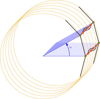
Figure 4. Example of a $3$-regular graphing that is not a strong local global limit.

Assume $\mathbf{G}$ is the strong local-global limit of a sequence $\boldsymbol{\mathsf{G}}=(G_{n})_{n\in\mathbb{N}}$ of graphs. Almost all neighborhoods in $G_{n}$ (for $n$ large) look the same: color red all vertices with two adjacent neighbors and color green all the vertices having exactly two non red neighbors.

Then, apart from a negligible set of vertices all the vertices are colored red and green. Moreover, almost all green vertices belong either to a long green cycle or a long green path. Recolor the green vertices in blue, green, and purple by dividing all these paths and cycles in almost equal parts (and taking care of globally balancing these colors). Now consider a local convergent subsequence of the colored $G_{n}$. By definition this local subsequence can be extended into a local convergent sequence $\boldsymbol{\mathsf{G^{+}}}$ of colorings of the graphs in $\boldsymbol{\mathsf{G}}$. By local convergence, every connected component of the sub-graphing induced by green, blue, and violet vertices are monochromatic (apart from a $0$ measure set), and these components are invariant by the transformation $(x,y)\mapsto(x+\alpha\bmod 1,y)$ (hence $y\in\{1,6\}$. However, this sub-graphing has two ergodic components, each of measure $1/6$ although each of the blue, green, and violet color contain asymptotically $1/9$ of the vertices, a contradiction.

4. Applications

4.1. Clustering

Monadic lifts (i.e. lifts by unary relations) were considered in [24] in the context of continuous clustering of the structures in an ${\rm FO}^{\rm local}$-convergent sequence. One of the main results (see Theorem 4.1.1 bellow) expresses that every ${\rm FO}^{\rm local}$-convergent sequence has monadic lift tracing components while preserving ${\rm FO}^{\rm local}$-convergence. This will be refined in this section under the stronger assumption of $\mathsf{Sh}_{*}({\rm FO}^{\rm local})$-convergence (see Theorem 4.1.6).

Figure 5. Typical shape of a structure continuously segmented by a clustering: dense spots correspond to globular clusters, and the background to the residual cluster. Biggest globular clusters appear first and then move apart from each other, while new (smaller) globular clusters appear and residual cluster becomes sparser and sparser.

The analysis in [24] leads to interesting notions: globular cluster (corresponding to a limit non-zero measure connected component), residual cluster (corresponding to all the zero-measure connected components taken as a whole), and negligible cluster (corresponding to the stretched part connecting the other clusters, which eventually disappears at the limit).

Negligible sets intuitively correspond to parts of the graph one can remove, without a great modification of the statistics of the graph: A sequence $\mathsf{X}\subseteq\mathsf{A}$ is negligible in a local-convergent sequence $\boldsymbol{\mathsf{A}}$ if

$$\forall d\in\mathbb{N}:\quad\limsup_{n\rightarrow\infty}\nu_{\mathbf{A}_{n}}({\rm N}_{\mathbf{A}_{n}}^{d}(X_{n}))=0.$$

This we simply formulate as $\forall d\in\mathbb{N}:\ \limsup\nu_{\boldsymbol{\mathsf{A}}}({\rm N}_{\boldsymbol{\mathsf{A}}}^{d}(\mathsf{X}))=0$.

Two sequences $\mathsf{X}$ and $\mathsf{Y}$ of subsets are equivalent in $\boldsymbol{\mathsf{A}}$ if the sequence $\mathsf{X}\,\Delta\,\mathsf{Y}=(X_{n}\,\Delta\,Y_{n})_{n\in\mathbb{N}}$ is negligible in $\boldsymbol{\mathsf{A}}$. This will be denoted by $\mathsf{X}\approx\mathsf{Y}$. We denote by $\mathsf{0}$ the sequence of empty subsets. Hence $\mathsf{X}\approx\mathsf{0}$ is equivalent to the property that $\mathsf{X}$ is negligible. We further define a partial order on sequences of subsets by $\mathsf{X}\preceq\mathsf{Y}$ if the sequence $\mathsf{X}\setminus\mathsf{Y}=(X_{n}\setminus Y_{n})_{n\in\mathbb{N}}$ is negligible in $\boldsymbol{\mathsf{A}}$. Hence $\preceq$ has $\mathsf{0}$ for its minimum and $\mathsf{X}\approx\mathsf{Y}$ iff $\mathsf{X}\preceq\mathsf{Y}$ and $\mathsf{Y}\preceq\mathsf{X}$.

The notion of cluster of a local-convergent sequence is a weak analog of the notion of union of connected components, or more precisely of the topological notion of “clopen subset”: A sequence $\mathsf{X}$ of subsets of a local-convergent sequence $\boldsymbol{\mathsf{A}}$ is a cluster of $\boldsymbol{\mathsf{A}}$ if the following conditions hold:

1. the lifted sequence ${\rm L}_{\mathsf{X}}(\boldsymbol{\mathsf{A}})$ obtained by marking set $X_{n}$ in $\mathbf{A}_{n}$ by a new unary relation $M_{\mathsf{X}}$ is local-convergent;

2. the sequence $\partial_{\boldsymbol{\mathsf{A}}}\mathsf{X}$ is negligible in $\boldsymbol{\mathsf{A}}$.

Condition (1) can be seen as a continuity requirement for the subset selection. Condition (2) is stronger than the usual requirement that there are not too many connections leaving the cluster. We intuitively require that the (asymptotically arbitrarily large) ring around a cluster is a very sparse zone.

A cluster $\mathsf{X}$ is atomic if, for every cluster $\mathsf{Y}$ of $\boldsymbol{\mathsf{A}}$ such that $\mathsf{Y}\preceq\mathsf{X}$ either $\mathsf{Y}\approx\mathsf{0}$ or $\mathsf{Y}\approx\mathsf{X}$; the cluster $\mathsf{X}$ is strongly atomic if $\mathsf{X}_{f}$ is an atomic cluster of $\boldsymbol{\mathsf{A}}_{f}$ for every increasing function $f:\mathbb{N}\rightarrow\mathbb{N}$. To the opposite, the cluster $\mathsf{X}$ is a nebula if, for every increasing function $f:\mathbb{N}\rightarrow\mathbb{N}$, every atomic cluster $\mathsf{Y}_{f}$ of $\boldsymbol{\mathsf{A}}_{f}$ with $\mathsf{Y}_{f}\subseteq\mathsf{X}_{f}$ is trivial (i.e. $\mathsf{Y}_{f}\approx\mathsf{0}$). Finally, a cluster $\mathsf{X}$ is universal for $\boldsymbol{\mathsf{A}}$ if $\mathsf{X}$ is a cluster of every conservative lift of $\boldsymbol{\mathsf{A}}$.

Two clusters $\mathsf{X}$ and $\mathsf{Y}$ of a local-convergent sequence $\boldsymbol{\mathsf{A}}$ are interweaving, and we note $\mathsf{X}\between\mathsf{Y}$ if every sequence $\mathsf{Z}$ with $Z_{n}\in\{X_{n},Y_{n}\}$ is a cluster of $\boldsymbol{\mathsf{A}}$.

We say that two clusters $\mathsf{C_{1}}$ and $\mathsf{C_{2}}$ are

• weakly disjoint if $\mathsf{C_{1}}\cap\mathsf{C_{2}}\approx\mathsf{0}$;

• disjoint if $\mathsf{C_{1}}\cap\mathsf{C_{2}}=\mathsf{0}$;

• strongly disjoint if $({\rm N}_{\boldsymbol{\mathsf{A}}}(\mathsf{C_{1}})\cap\mathsf{C_{2}})\cup(\mathsf{C_{1}}\cap{\rm N}_{\boldsymbol{\mathsf{A}}}(\mathsf{C_{2}}))=\mathsf{0}$.

A cluster $\mathsf{C}$ of a local-convergent sequence $\boldsymbol{\mathsf{A}}$ is globular if, for every $\epsilon>0$ there exists $d\in\mathbb{N}$ such that

$$\adjustlimits{\liminf}_{n\rightarrow\infty}{\sup}_{v_{n}\in C_{n}}\nu_{\mathbf{A}_{n}}({\rm N}_{\mathbf{A}_{n}}^{d}(v_{n}))>(1-\epsilon)\lim_{n\rightarrow\infty}\nu_{\mathbf{A}_{n}}(C_{n}).$$

In other words, a cluster $\mathsf{C}$ is globular if, for every $\epsilon>0$ and sufficiently large $n$, $\epsilon$-almost all elements of $C_{n}$ are included in some ball of radius at most $d$ in $C_{n}$, for some fixed $d$. (Note that for a cluster $\mathsf{C}$ and $v_{n}\in C_{n}$, considering $\nu_{\mathbf{A}_{n}}({\rm N}_{\mathbf{A}_{n}}^{d}(v_{n}))$ or $\nu_{\mathbf{A}_{n}}({\rm N}_{\mathbf{A}_{n}[C_{n}]}^{d}(v_{n}))$ makes asymptotically no difference.) Every globular cluster is clearly strongly atomic, but the converse does not hold as witnessed, for instance, by sequence of expanders. The strongly atomic clusters that are not globular are called open clusters. Opposite to globular clusters are residual clusters: A cluster $\mathsf{X}$ of $\boldsymbol{\mathsf{A}}$ is residual if for every $d\in\mathbb{N}$ it holds

$$\adjustlimits{\limsup}_{n\rightarrow\infty}{\sup}_{v_{n}\in A_{n}}\nu_{\mathbf{A}_{n}}({\rm N}_{\mathbf{A}_{n}}^{d}(v_{n}))=0.$$

Theorem 4.1.1 ([24]).

Let $\boldsymbol{\mathsf{A}}$ be a local convergent sequence of $\sigma$-structures. Then there exists a signature $\sigma^{+}$ obtained from $\sigma$ by the addition of countably many unary symbols $M_{R}$ and $M_{i,j}$ ($i\in\mathbb{N}$, $1\leq j\leq N_{i}$) and a clustering $\boldsymbol{\mathsf{A}}^{+}$ of $\boldsymbol{\mathsf{A}}$ with the following properties:

• For every $i\in\mathbb{N}$, $\bigcup_{j=1}^{N_{i}}M_{i,j}(\boldsymbol{\mathsf{A}})$ is a universal cluster;

• For every $i\in\mathbb{N}$ and every $1\leq j\leq N_{i}$, $M_{i,j}(\boldsymbol{\mathsf{A}})$ is a globular cluster;

• Two clusters $M_{i,j}(\boldsymbol{\mathsf{A}})$ and $M_{i^{\prime},j^{\prime}}(\boldsymbol{\mathsf{A}})$ are interweaving if and only if $i=i^{\prime}$;

• $M_{R}(\boldsymbol{\mathsf{A}})$ is a residual cluster.

This structural theorem is assuming the local convergence of the sequence. If we assume local-global convergence we get stronger results (Theorem 4.1.6 bellow) involving expanding properties which we will define now. This is pleasing as the decomposition into expanders was one of the motivating examples [6] and [12].

The following is a sequential version of expansion property: A structure $\mathbf{A}$ is $(d,\epsilon,\delta)$-expanding if, for every $X\subset A$ it holds

$$\epsilon<\nu_{\mathbf{A}}(X)<1-\epsilon\quad\Longrightarrow\quad\nu_{\mathbf{A}}({\rm N}_{\mathbf{A}}^{d}(X))>(1+\delta)\nu_{\mathbf{A}}(X).$$

This condition may be reformulated as:

$$\inf\biggl{\{}\frac{\nu_{\mathbf{A}}({\rm N}_{\mathbf{A}}^{d}(X)\setminus X)}{\nu_{\mathbf{A}}(X)}:\quad\epsilon<\nu_{\mathbf{A}}(X)<1-\epsilon\biggr{\}}>\delta.$$

Note that the left hand size of the above inequality is similar to the magnification introduced in [3], which is the isoperimetric constant $h_{\rm out}$ defined by

$$h_{\rm out}=\inf\left\{\frac{|{\rm N}_{\mathbf{A}}(X)\setminus X|}{|X|}:\quad 0<\frac{|X|}{|A|}<1/2\right\}.$$

A local-convergent sequence $\boldsymbol{\mathsf{A}}$ is expanding if, for every $\epsilon>0$ there exist $d,t\in\mathbb{N}$ and $\delta>0$ such that every $\mathbf{A}_{n}$ with $n\geq t$ is $(d,\epsilon,\delta)$-expanding. A non-trivial cluster $\mathsf{X}$ of $\boldsymbol{\mathsf{A}}$ is expanding of $\boldsymbol{\mathsf{A}}$ if $\boldsymbol{\mathsf{A}}[\mathsf{X}]$ is expanding. We have the following equivalent formulations of this concept:

Lemma 4.1.2 ([24]).

Let $\mathsf{X}\not\approx\mathsf{0}$ be a cluster of a local convergent sequence $\boldsymbol{\mathsf{A}}$. The following conditions are equivalent:

1. $\mathsf{X}$ is an expanding cluster of $\boldsymbol{\mathsf{A}}$;

2. for every $\epsilon>0$ there exists $d,t\in\mathbb{N}$ such that for every $\mathsf{Z}\subseteq\mathsf{X}$ with $\nu_{\boldsymbol{\mathsf{A}}}(\mathsf{Z})>\epsilon\nu_{\boldsymbol{\mathsf{A}}}(\mathsf{X})$ it holds

   $$\nu_{\boldsymbol{\mathsf{A}}}({\rm N}_{\boldsymbol{\mathsf{A}}}^{d}(\mathsf{Z}))>(1-\epsilon)\nu_{\boldsymbol{\mathsf{A}}}(\mathsf{X});$$

3. the sequence $\mathsf{X}$ is a strongly atomic cluster of $\boldsymbol{\mathsf{A}}$;

4. for every $\epsilon>0$ there exists no $\mathsf{Y}\subseteq\mathsf{X}$ such that $\partial_{\boldsymbol{\mathsf{A}}}\mathsf{Y}\approx\mathsf{0}$ and

   $$\epsilon<\liminf\nu_{\boldsymbol{\mathsf{A}}}(\mathsf{Y})<\lim\nu_{\boldsymbol{\mathsf{A}}}(\mathsf{X})-\epsilon.$$

Note that for local-global convergent sequences, the notions of atomic, strongly atomic, and expanding clusters are equivalent.

The case of bounded degree graphs is particularly interesting and our definitions capture this as well. Recall that a sequence $\boldsymbol{\mathsf{G}}$ of graphs is a vertex expander if there exists $\alpha>0$ such that $\liminf h_{\rm out}(G_{n})\geq\alpha$. (For more information on expanders we refer the reader to [15].)

Lemma 4.1.3 ([24]).

Let $\boldsymbol{\mathsf{G}}$ be a sequence of graphs with maximum degree at most $\Delta$ and let $\mathsf{C}\not\approx\mathsf{0}$ be a cluster of $\boldsymbol{\mathsf{G}}$. The following are equivalent:

• $\mathsf{C}$ is an expanding cluster;

• for every $\epsilon>0$ there exists $\mathsf{X}\subseteq\mathsf{C}$ such that for every $n\in\mathbb{N}$ it holds $|X_{n}|<\epsilon|C_{n}|$ and $\boldsymbol{\mathsf{G}}[\mathsf{C}\setminus\mathsf{X}]$ is a vertex expander.

We consider a fixed enumeration $\phi_{1},\phi_{2},\dots$ of ${\rm FO}^{\rm local}$. The profile ${\rm Prof}(\mathsf{C})$ of a cluster $\mathsf{C}$ is the sequence formed by $\lim\nu_{\boldsymbol{\mathsf{A}}}(\mathsf{C})$ followed by the values $\lim\langle\phi_{i},\boldsymbol{\mathsf{A}}[\mathsf{C}]\rangle$ for $i\in\mathbb{N}$. The lexicographic order on the profiles is denoted by $\leq$.

In [24] it was proved that two expanding clusters are either weakly disjoint or interweaving. We now prove a lemma with similar flavor.

Lemma 4.1.4.

Let $\mathsf{C}_{1}$ be an expanding cluster of a local-convergent sequence $\boldsymbol{\mathsf{A}}$ and let $\mathsf{C}_{2}$ be a cluster of $\boldsymbol{\mathsf{A}}$.

Then the limit set of $\nu_{\boldsymbol{\mathsf{A}}}(\mathsf{C}_{1}\cap\mathsf{C}_{2})$ is included in $\{0,\lim\nu_{\boldsymbol{\mathsf{A}}}(\mathsf{C}_{1})\}$.

Proof.

Let $\mathsf{X}=\mathsf{C_{1}}\cap\mathsf{C_{2}}$. Assume for contradiction that there exists $0<\alpha<\lim\nu_{\boldsymbol{\mathsf{A}}}(\mathsf{C}_{1})$ and a subsequence $\boldsymbol{\mathsf{A}}_{f}$ such that ${\rm L}_{\mathsf{X}_{f}}(\boldsymbol{\mathsf{A}}_{f})$ is local convergent and $\lim\nu_{\boldsymbol{\mathsf{A}}_{f}}(\mathsf{X}_{f})=\alpha$. As $\delta_{\boldsymbol{\mathsf{A}}}\mathsf{X}\subseteq\delta_{\boldsymbol{\mathsf{A}}}\mathsf{C}_{1}\cup\delta_{\boldsymbol{\mathsf{A}}}\mathsf{C}_{2}$ we deduce that $\mathsf{X}_{f}$ is a cluster of $\boldsymbol{\mathsf{A}}_{f}$. But $\mathsf{X}_{f}\subseteq(\mathsf{C}_{1})_{f}$, $\mathsf{X}_{f}\not\approx\mathsf{0}$, and $\mathsf{X}_{f}\not\approx\mathsf{C}_{1}$ (as $\lim\nu_{\boldsymbol{\mathsf{A}}_{f}}(\mathsf{X}_{f})\notin\{0,\lim\nu_{\boldsymbol{\mathsf{A}}}(\mathsf{C}_{1})\}$), what contradicts the hypothesis that $\mathsf{C}_{1}$ is expanding hence strongly atomic (see Lemma 4.1.2). ∎

The following lemma is a restated version of a Lemma proved in [24].

Lemma 4.1.5.

Two non-negligible clusters $\mathsf{C_{1}}$ and $\mathsf{C_{2}}$ are interweaving if and only if ${\rm Profile}(\mathsf{C_{1}})={\rm Profile}(\mathsf{C_{2}})$.∎

Our main result in this section reveals the expanding structure of local-global convergent sequences.

Theorem 4.1.6.

Let $\sigma$ be a countable relational signature, let $\sigma^{+}$ be the extension of $\sigma$ by countably many unary symbols $N$ and $U_{i}$ ($i\in\mathbb{N}$), and let $\sigma^{*}$ be the extension of $\sigma$ by countably many unary symbols $N$ and $M_{i,j}$. Let $\mathsf{I}:\sigma^{*}\rightarrow\sigma^{+}$ be the basic interpretation defined by $\rho_{U_{i}}(x):=\bigvee M_{i,j}(x)$ (and all other relations unchanged), and let $\mathsf{Sh}^{*}:\sigma^{*}\rightarrow\sigma$ and $\mathsf{Sh}^{+}:\sigma^{+}\rightarrow\sigma$ be the natural forgetful interpretations.

Then for every local-global convergent sequence $\boldsymbol{\mathsf{A}}$ of $\sigma$-structure there exists a local-convergent sequence $\boldsymbol{\mathsf{A}}^{*}$ such that

• $P(\mathsf{Sh}^{*})(\boldsymbol{\mathsf{A}}^{*})=\boldsymbol{\mathsf{A}}$,

• for every $i,j\in\mathbb{N}$, $M_{i,j}(\boldsymbol{\mathsf{A}}^{*})$ is either null or an atomic cluster of $\boldsymbol{\mathsf{A}}^{*}$, which is interweaving with $M_{i^{\prime},j^{\prime}}(\boldsymbol{\mathsf{A}}^{*})$ if and only if $i=i^{\prime}$,

• $N(\boldsymbol{\mathsf{A}}^{*})$ is a nebula cluster of $\boldsymbol{\mathsf{A}}^{*}$,

and such that $\boldsymbol{\mathsf{A}}^{+}=P(\mathsf{I})(\boldsymbol{\mathsf{A}}^{*})$ has the following properties:

• $\boldsymbol{\mathsf{A}}^{+}$ is a local-global convergent sequence such that $P(\mathsf{Sh}^{+})(\boldsymbol{\mathsf{A}}^{+})=\boldsymbol{\mathsf{A}}$,

• for every $i\in\mathbb{N}$, $U_{i}(\boldsymbol{\mathsf{A}}^{+})$ is either null or a cluster of $\boldsymbol{\mathsf{A}}^{+}$, which can be covered by (finitely many) interweaving atomic clusters,

• $N(\boldsymbol{\mathsf{A}}^{+})$ is a nebula cluster of $\boldsymbol{\mathsf{A}}^{+}$.

Note that this result is in agreement with the intuition: The $\sigma^{*}$-lift is “finer” than the $\sigma^{+}$-lift and thus less likely to be local-global convergent. For instance, we can refer to the subsequence extension property stated in the definition of lift-Hausdorff convergence (Definition 3.3.1).

Proof.

Let $\boldsymbol{\mathsf{A}}$ be a local-global convergent sequence. We select inductively clusters expanding clusters $\mathsf{C}^{i,j}$ of $\boldsymbol{\mathsf{A}}$ as follows: We start with $\mathsf{Z}=\mathsf{0}$, $i=1$, $j=1$ and let $P$ be the maximum profile of an expanding cluster of $\boldsymbol{\mathsf{A}}$. Then we repeat the following procedure as long as there exists an expanding cluster of $\boldsymbol{\mathsf{A}}$ that is weakly disjoint from $\mathsf{Z}$

• If there exists an expanding cluster in $\boldsymbol{\mathsf{A}}$ with profile $P$ that is weakly disjoint from $\mathsf{Z}$ we select one as $\mathsf{C}^{i,j}$, we let $\mathsf{Z}\leftarrow\mathsf{Z}\cup\mathsf{C}^{i,j}$, and we increase $j$ by $1$.

• Otherwise, we select one with maximum profile as $\mathsf{C}^{i+1,1}$, e let $\mathsf{Z}\leftarrow\mathsf{Z}\cup\mathsf{C}^{i+1,1}$, we let $P$ be the profile of $\mathsf{C}^{i+1,1}$, we increase $i$ by $1$, and let $j=1$.

It is easily checked that by modifying marginally the clusters $\mathsf{C}^{i,j}$ we can make them disjoint and such that $\mathsf{N}=\mathsf{A}\setminus\bigcup_{i,j}\mathsf{C}^{i,j}$ is a nebula cluster. Then by [24, Corollary 5] lifting $\boldsymbol{\mathsf{A}}$ by marking $M_{i,j}$ the cluster $\mathsf{C}^{i,j}$ and $N$ the cluster $\mathsf{N}$ we get a local-convergent sequence $\boldsymbol{\mathsf{A}}^{*}$, which obviously satisfies the conditions stated in the Theorem.

Let $\boldsymbol{\mathsf{A}}^{+}=P(\mathsf{I})(\boldsymbol{\mathsf{A}}^{*})$. The only property we still have to prove is that $\boldsymbol{\mathsf{A}}^{+}$ is local-global convergent. According to Definition 3.3.1 this boils down to proving that every local-convergent subsequence $\boldsymbol{\mathsf{B}}^{+}_{f}$ of lifts of $\boldsymbol{\mathsf{A}}^{+}$ can be extended into a full local-convergent sequence of lifts of $\boldsymbol{\mathsf{A}}^{+}$. We can transfer the relations $M_{i,j}$ from $\boldsymbol{\mathsf{A}}^{*}$ to $\boldsymbol{\mathsf{B}}^{+}_{f}$. This way we obtain a subsequence $\boldsymbol{\mathsf{B}}^{*}_{f}$ of lifts of $\boldsymbol{\mathsf{A}}^{*}$ (which does not need to be local convergent), such that $P(\mathsf{I})(\boldsymbol{\mathsf{B}}^{*}_{f})=\boldsymbol{\mathsf{B}}^{+}_{f}$. Let $\boldsymbol{\mathsf{B}}^{*}_{g\circ f}$ be a local-convergent subsequence of $\boldsymbol{\mathsf{B}}^{*}_{f}$. As $P(\mathsf{Sh}^{*})(\boldsymbol{\mathsf{B}}^{*}_{g\circ f})=\boldsymbol{\mathsf{A}}_{g\circ f}$ and $\boldsymbol{\mathsf{A}}$ is local-global convergent there exists a local-convergent sequence $\boldsymbol{\mathsf{D}}^{*}$ of lifts of $\boldsymbol{\mathsf{A}}$ extending $\boldsymbol{\mathsf{B}}^{*}_{g\circ f}$, that is: $P(\mathsf{Sh}^{*})(\boldsymbol{\mathsf{D}}^{*})=\boldsymbol{\mathsf{A}}$ and $\boldsymbol{\mathsf{D}}^{*}_{g\circ f}=\boldsymbol{\mathsf{B}}^{*}_{g\circ f}$. Let $\hat{\mathsf{C}}^{i,j}=M_{i,j}(\boldsymbol{\mathsf{D}}^{*})$. As $(\hat{\mathsf{C}}^{i,j})_{g\circ f}=(\mathsf{C}^{i,j})_{g\circ f}$ we get that $\hat{\mathsf{C}}^{i,j}$ is a cluster of $\boldsymbol{\mathsf{A}}$ with same profile as $\mathsf{C}^{i,j}$. According to Lemma 4.1.4, the limit set of $\nu_{\boldsymbol{\mathsf{A}}}(\hat{\mathsf{C}}^{i,j}\cap\mathsf{C}^{i,j^{\prime}})$ is included in $\{0,m\}$, where $m=\lim\nu_{\boldsymbol{\mathsf{A}}}(\hat{\mathsf{C}}^{i,j})=\lim\nu_{\boldsymbol{\mathsf{A}}}(\mathsf{C}^{i,j^{\prime}})$. It follows that either $\hat{\mathsf{C}}^{i,j}\preceq\bigcup_{j^{\prime}}\mathsf{C}^{i,j^{\prime}}$ or there exists a subsequence $\boldsymbol{\mathsf{A}}_{h}$ of $\boldsymbol{\mathsf{A}}$ such that $(\hat{\mathsf{C}}^{i,j})_{h}$ is weakly disjoint from the cluster $(\bigcup_{j^{\prime}}\mathsf{C}^{i,j^{\prime}})_{g}$. Marking all the clusters $\mathsf{C}^{i,j}$ and $\hat{\mathsf{C}}^{i,j}$ in $\boldsymbol{\mathsf{A}}_{h}$ we get a local-convergent subsequence of lifts, which can be extended into full local-convergent sequence of lifts of $\boldsymbol{\mathsf{A}}$. In this sequence, the marks corresponding to the extension of $(\hat{\mathsf{C}}^{i,j})_{g}$ will correspond to a cluster of $\boldsymbol{\mathsf{A}}$ disjoint from all the clusters $\mathsf{C}^{i,j^{\prime}}$ but with the same profile, which contradicts the construction procedure of the clusters $\mathsf{C}^{i,j}$. Thus $\hat{\mathsf{C}}^{i,j}\preceq\bigcup_{j^{\prime}}\mathsf{C}^{i,j^{\prime}}$, and $\bigcup_{j}\hat{\mathsf{C}}^{i,j}\preceq\bigcup_{j^{\prime}}\mathsf{C}^{i,j^{\prime}}$. As these two clusters have same limit measure we have $\bigcup_{j}\hat{\mathsf{C}}^{i,j}\approx\bigcup_{j^{\prime}}\mathsf{C}^{i,j^{\prime}}$. This means that $P(\mathsf{I})(\boldsymbol{\mathsf{D}}^{*})$ and $P(\mathsf{I})(\boldsymbol{\mathsf{B}}^{*})$ are sufficiently close, so that if we consider the lifts of $\boldsymbol{\mathsf{A}}^{+}$ defined by $\boldsymbol{\mathsf{B}}^{+}$ for indices of the form $f(n)$ for some $n\in\mathbb{N}$ and by $P(\mathsf{I})(\boldsymbol{\mathsf{D}}^{*})$ for the other indices, we get a local-convergent sequence of lifts of $\boldsymbol{\mathsf{A}}^{+}$ which extends $\boldsymbol{\mathsf{B}}^{+}_{f}$. It follows that $\boldsymbol{\mathsf{A}}^{+}$ is local-global convergent, what concludes our proof. ∎

4.2. Local Global Quasi-Limits

Let us finish this paper in an ambitious way. In [25, 22] we defined the notion of modeling as a limit object from structural convergence.

Modeling limits generalize graphing limits and thus it follows from [20] that ${\rm FO}$-convergent sequences of graphs with bounded degrees have modeling limits. In [25] we constructed modeling limits for ${\rm FO}$-convergent sequences of graphs with bounded tree-depth, and extended the construction to ${\rm FO}$-convergent sequences of trees in [22]. Then existence of modelings for ${\rm FO}$-convergent sequences has been proved for graphs with bounded path-width [11] and eventually for sequences of graphs in an arbitrary nowhere dense class [26], which is best possible when considering monotone classes of graphs [22]. In fact this provides us with a high level analytic characterization of nowhere dense classes.

Definition 4.2.1.

Let $\boldsymbol{\mathsf{A}}$ be a local-global convergent sequence. A modeling $\mathbf{L}$ is a local-global quasi-limit of $\boldsymbol{\mathsf{A}}$ if for every local convergent sequence $\boldsymbol{\mathsf{A^{+}}}$ of lifts of $\boldsymbol{\mathsf{A}}$ and every $\epsilon>0$ there exists an admissible lift $\mathbf{L}^{+}$ of $\mathbf{L}$ (that is a lift $\mathbf{L}^{+}$ of $\mathbf{L}$ that is a modeling), such that for every local formula $\phi$ we have

$$\bigl{|}\langle\phi,\mathbf{L}^{+}\rangle-\lim_{n\rightarrow\infty}\langle\phi,\mathbf{A}_{n}^{+}\rangle\bigr{|}<c_{\phi}\epsilon,$$

where $c_{\phi}$ is a positive constant, which depends only on $\phi$.

In other words, the closure of the measures associated to admissible lifts of $\mathbf{L}$ includes the limit Hausdorff limit of the sets of measures associated to lifts of the sequence.

For local-global convergence, it was proved in [12] that graphings still suffice as limit objects. We don’t know, however, if every local-global convergent sequence of graphs in a nowhere dense class has a modeling local-global limit. We close this paper by proving that this is almost the case, in the sense that every local-global convergent sequence of graphs in a nowhere dense class has a modeling local-global quasi-limit.

We consider a fixed countable signature $\sigma$ and the signature $\tau$ obtained by adding countably many unary symbols $M_{1},M_{2},\dots,M_{n},\dots$ to $\sigma$, and the forgetful interpretation $\mathsf{Sh}:\tau\rightarrow\sigma$. As before we understand local-global convergence as $\mathsf{Sh}_{*}({\rm FO}^{\rm local})$-convergence. We fix a chain covering $\mathfrak{X}$ of ${\rm FO}^{\rm local}(\tau)$ (see Section 2.5), from which we derive metrics and pseudo-metrics as in Sections 3.2 and 3.3. We also fix a bijection $\beta:\mathbb{N}\times\mathbb{N}\rightarrow\mathbb{N}$ (for Hilbert hotel argument) and let $Z_{c}$ be the renaming interpretation which renames $M_{\beta(c,i)}$ as $M_{i}$ and forget all the marks not being renamed.

Lemma 4.2.2.

There exists a function $h:(0,1)\rightarrow\mathbb{N}$ with the following property:

For every local-global convergent sequence $\boldsymbol{\mathsf{A}}$ of $\sigma$-structures there exists a local convergent sequence $\boldsymbol{\mathsf{B}}$ of $\tau$-structures with $P(\mathsf{Sh})(\boldsymbol{\mathsf{B}})=\boldsymbol{\mathsf{A}}$, such that for every $\epsilon>0$ there exists some integer $n_{0}$ such that

for every $n\geq n_{0}$ and every $\mathbf{C}\in P(\mathsf{Sh})^{-1}(\mathbf{A}_{n})$ there exists $1\leq c\leq h(\epsilon)$ with

$${\rm dist}_{\mathfrak{X}}(\mathbf{C},P(\mathsf{Z}_{c})(\mathbf{B}_{n}))<\epsilon.$$

Proof.

As the space $({\rm Rel}(\tau),{\rm dist}_{\mathfrak{X}})$ is totally bounded there exists a mapping $g:(0,1)\rightarrow\mathbb{N}$ such that for each $\epsilon>0$ and each $\sigma$-structure $\mathbf{A}$ there is a subset $\mathcal{B}_{\mathbf{A},\epsilon}$ of $P(\mathsf{Sh})^{-1}(\mathbf{A})$ of cardinality at most $g(\epsilon)$ with the property that every $\mathbf{C}\in P(\mathsf{Sh})^{-1}(\mathbf{A})$ is at ${\rm dist}_{\mathfrak{X}}$-distance at most $\epsilon$ from a $\tau$-structure in $\mathcal{B}_{\mathbf{A},\epsilon}$. (Such a set may be called an $\epsilon$-covering.) We construct an infinite sequence $(\mathbf{A}^{(i)})_{i\in\mathbb{N}}$ of $\tau$-structures by listing all the structures in $\mathcal{B}_{\mathbf{A},1/2}$ then all the structures in $\mathcal{B}_{\mathbf{A},1/4}$, etc.

We now construct a $\tau$-structure $\mathbf{A}^{+}\in P(\mathsf{Sh})^{-1}(\mathbf{A})$ by letting $M_{\beta(i,j)}(\mathbf{A}^{+})=M_{j}(\mathbf{A}^{(i)})$. Hence $\mathbf{A}^{(i)}=P(\mathsf{Z}_{i})(\mathbf{A}^{+})$. We say that $\mathbf{A}^{+}$ is a universal lift of $\mathbf{A}$.

Define the function $h:(0,1)\rightarrow\mathbb{N}$ by

$$h(x)=\sum_{i=1}^{\lceil-\log x\rceil+1}g(2^{-i}).$$

Then for every $\epsilon>0$ and every $\mathbf{B}\in P(\mathsf{Sh})^{-1}(\mathbf{A})$ there is an index $c\leq h(\epsilon)$ such that ${\rm dist}_{\mathfrak{X}}(\mathbf{C},\mathbf{A}^{(c)})<\epsilon/2$, that is such that ${\rm dist}_{\mathfrak{X}}(\mathbf{C},P(\mathsf{Z}_{c})(\mathbf{A}^{+}))<\epsilon/2$.

Now consider the local-global convergent sequence $\boldsymbol{\mathsf{A}}$ and a sequence $\boldsymbol{\mathsf{A}}^{+}$ where $\mathbf{A}_{n}^{+}$ is a universal lift of $\mathbf{A}_{n}$. This last sequence has a local convergent subsequence $\boldsymbol{\mathsf{A}}^{+}_{f}$, which we extend into a sequence $\boldsymbol{\mathsf{B}}$ lifting $\boldsymbol{\mathsf{A}}$.

Let $\epsilon>0$. According to local-global convergence of $\boldsymbol{\mathsf{A}}$ and local convergence of $\boldsymbol{\mathsf{B}}$ there exists $n_{0}$ such that for every $n,m\geq n_{0}$ we have ${\rm dist}_{\mathfrak{X},\mathsf{Sh}}^{\rm H}(\mathbf{A}_{n},\mathbf{A}_{m})<\epsilon/4$ and ${\rm dist}_{\mathfrak{X}}(\mathbf{B}_{n},\mathbf{B}_{m})<\alpha$, where $\alpha$ is such that for every $i\leq h(\epsilon/2)$ we have

$${\rm dist}_{\mathfrak{X}}(\mathbf{X},\mathbf{Y})<\alpha\Rightarrow{\rm dist}_{\mathfrak{X}}(P(\mathsf{Z}_{i})(\mathbf{X}),P(\mathsf{Z}_{i})(\mathbf{Y}))<\epsilon/4.$$

Let $n\geq n_{0}$ (hence $f(n)\geq n_{0}$). Let $\mathbf{C}\in P(\mathsf{Sh})^{-1}(\mathbf{A}_{n})$. Then there exists $\mathbf{C}^{\prime}\in P(\mathsf{Sh})^{-1}(\mathbf{A}_{f(n)})$ such that ${\rm dist}_{\mathfrak{X}}(\mathbf{C},\mathbf{C}^{\prime})<\epsilon/4$. As $\mathbf{B}_{f(n)}=\mathbf{A}_{f(n)}^{+}$ is a universal lift of $\mathbf{A}_{f(n)}$ there exists $c\leq h(\epsilon)$ such that ${\rm dist}_{\mathfrak{X}}(P(\mathsf{Z}_{c})(\mathbf{B}_{f(n)}),\mathbf{C}^{\prime})<\epsilon/2$. As ${\rm dist}_{\mathfrak{X}}(\mathbf{B}_{n},\mathbf{B}_{f(n)})<\alpha$ we have ${\rm dist}_{\mathfrak{X}}(P(\mathsf{Z}_{c})(\mathbf{B}_{f(n)}),P(\mathsf{Z}_{c})(\mathbf{B}_{n})<\epsilon/4$. Altogether, we get ${\rm dist}_{\mathfrak{X}}(P(\mathsf{Z}_{c})(\mathbf{B}_{n}),\mathbf{C})<\epsilon$ as wanted. ∎

Definition 4.2.3.

A $\sigma$-modeling $\mathbf{L}$ is a quasi-limits of a local global convergent sequence $\boldsymbol{\mathsf{A}}$ of $\sigma$-structures if, for every local convergent sequence $\boldsymbol{\mathsf{A}}^{+}$ of $\tau$-structures with $P(\mathsf{Sh})(\boldsymbol{\mathsf{A}}^{+})=\boldsymbol{\mathsf{A}}$ and for every $\epsilon>0$ there exists a $\tau$-modeling $\mathbf{L}^{+}$ with $P(\mathsf{Sh})(\mathbf{L}^{+})=\mathbf{L}$ such that $\limsup{\rm dist}_{\mathfrak{X}}(\mathbf{L}^{+},\boldsymbol{\mathsf{A}}^{+})<\epsilon$.

In other words, for every local-global convergent sequence $\boldsymbol{\mathsf{A}}$ there is a modeling $\mathbf{L}$ such that any local convergent sequence lifting $\boldsymbol{\mathsf{A}}$ has a limit which is $\epsilon$-close to an admissible lifting of $\mathbf{L}$. (By admissible, we mean that the lift of $\mathbf{L}$ is itself a modeling.)

Theorem 4.2.4.

Every local-global convergent sequence of graphs in a nowhere dense class has a modeling quasi-limit.

Proof.

Let $\boldsymbol{\mathsf{A}}$ be a local-global convergent of graphs in a nowhere dense class. According to Lemma 4.2.2 there exists a local convergent sequence $\boldsymbol{\mathsf{B}}$ of marked graphs with $P(\mathsf{Sh})(\boldsymbol{\mathsf{B}})=\boldsymbol{\mathsf{A}}$, such that for every $\epsilon>0$ there exists some integer $n_{0}$ such that for every $n\geq n_{0}$ and every $\mathbf{C}\in P(\mathsf{Sh})^{-1}(\mathbf{A}_{n})$ there exists $1\leq c\leq h(\epsilon)$ with

$${\rm dist}_{\mathfrak{X}}(\mathbf{C},P(\mathsf{Z}_{c})(\mathbf{B}_{n}))<\epsilon.$$

According to [26] the sequence $\boldsymbol{\mathsf{B}}$ has a modeling limit $\mathbf{L}^{+}$. Then $\mathbf{L}=P(\mathsf{Sh}(\mathbf{L}^{+})$ is a modeling quasi-limit of $\boldsymbol{\mathsf{A}}$. ∎

We conjecture that it is possible to refine the notion of admissible lift and get the reverse direction.

Conjecture 4.2.5.

Every local-global convergent sequence of graphs in a nowhere dense class has a modeling limit.

References

• [1] H. Adler and I. Adler, Interpreting nowhere dense graph classes as a classical notion of model theory, European Journal of Combinatorics 36 (2014), 322–330.
• [2] D. Aldous, Representations for partially exchangeable arrays of random variables, Journal of Multivariate Analysis 11 (1981), 581–598.
• [3] N. Alon, Eigenvalues and expanders, Combinatorica 6 (1986), no. 2, 83–96.
• [4] B. Balcar, T. Jech, and T. Pazák, Complete CCC Boolean algebras, the order sequential topology, and a problem of Von Neumann, Bulletin of the London Mathematical Society 37 (2005), no. 6, 885–898.
• [5] I. Benjamini and O. Schramm, Recurrence of distributional limits of finite planar graphs, Electronic Journal of Probability 6 (2001), no. 23, 13pp.
• [6] B. Bollobás and O. Riordan, Sparse graphs: metrics and random models, Random Structures & Algorithms 39 (2011), no. 1, 1–38.
• [7] C. Borgs, J.T. Chayes, and L Lovász, Moments of two-variable functions and the uniqueness of graph limits, Geometric And Functional Analysis 19 (2012), no. 6, 1597–1619.
• [8] C. Borgs, J.T. Chayes, L. Lovász, V.T. Sós, B. Szegedy, and K. Vesztergombi, Graph limits and parameter testing, STOC’06. Proceedings of the 38th Annual ACM Symposium on Theory of Computing, 2006, pp. 261–270.
• [9] C. Borgs, J.T. Chayes, L. Lovász, V.T. Sós, and K. Vesztergombi, Convergent sequences of dense graphs I: Subgraph frequencies, metric properties and testing, Advances in Mathematics 219 (2008), no. 6, 1801–1851.
• [10] by same author, Convergent sequences of dense graphs II: Multiway cuts and statistical physics, Annals of Mathematics 176 (2012), 151–219.
• [11] J. Gajarský, P. Hliněný, T. Kaiser, D. Kráľ, M. Kupec, J Obdržálek, S. Ordyniak, and V. Tůma, First order limits of sparse graphs: plane trees and path-width, Random Structures and Algorithms (2016).
• [12] H. Hatami, L. Lovász, and B. Szegedy, Limits of locally–globally convergent graph sequences, Geometric and Functional Analysis 24 (2014), no. 1, 269–296.
• [13] F. Hausdorff, Set theory, vol. 119, American Mathematical Soc., 1962.
• [14] W. Hodges, A shorter model theory, Cambridge University Press, 1997.
• [15] S. Hoory, N. Linial, and A. Wigderson, Expander graphs and their applications, Bulletin of the American Mathematical Society 43 (2006), no. 4, 439–561.
• [16] D. Hoover, Relations on probability spaces and arrays of random variables, Tech. report, Institute for Advanced Study, Princeton, NJ, 1979.
• [17] G. Kun and A. Thom, Almost automorphisms of sofic approximations, Borel combinatorics and ergodic theory conference (EPFL, CIB), 2018.
• [18] D. Lascar, La théorie des modèles en peu de maux, Cassini, 2009.
• [19] L. Lovász and B. Szegedy, Limits of dense graph sequences, Journal of Combinatorial Theory, Series B 96 (2006), 933–957.
• [20] J. Nešetřil and P. Ossona de Mendez, A model theory approach to structural limits, Commentationes Mathematicæ Universitatis Carolinæ 53 (2012), no. 4, 581–603.
• [21] by same author, First-order limits, an analytical perspective, European Journal of Combinatorics 52 Part B (2016), 368–388, Recent Advances in Graphs and Analysis (special issue).
• [22] by same author, Modeling limits in hereditary classes: Reduction and application to trees, Electronic Journal of Combinatorics 23 (2016), no. 2, #P2.52.
• [23] by same author, Structural sparsity, Uspekhi Matematicheskikh Nauk 71 (2016), no. 1, 85–116, (Russian Math. Surveys 71:1 79-107).
• [24] by same author, Cluster analysis of local convergent sequences of structures, Random Structures & Algorithms 51 (2017), no. 4, 674–728.
• [25] by same author, A unified approach to structural limits (with application to the study of limits of graphs with bounded tree-depth), Memoirs of the American Mathematical Society (2017), 117 pages; to appear.
• [26] by same author, Existence of modeling limits for sequences of sparse structures, The Journal of Symbolic Logic (2018), accepted.
• [27] P. Urysohn, Works on topology and other areas of mathematics 1, 2, State Publ. of Technical and Theoretical Literature, Moscow (1951).