Signatures of few-body resonances in finite volume

Abstract

We study systems of bosons and fermions in finite periodic boxes and show how the existence and properties of few-body resonances can be extracted from studying the volume dependence of the calculated energy spectra. We use and briefly review a plane-wave-based discrete variable representation, which allows a convenient implementation of periodic boundary conditions. With these calculations we establish that avoided level crossings occur in the spectra of up to four particles and can be linked to the existence of multibody resonances. To benchmark our method we use two-body calculations, where resonance properties can be determined with other methods, as well as a three-boson model interaction known to generate a three-boson resonance state. Finding good agreement for these cases, we then predict three-body and four-body resonances for models using a shifted Gaussian potential. Our results establish few-body finite-volume calculations as a new tool to study few-body resonances. In particular, the approach can be used to study few-neutron systems, where such states have been conjectured to exist.

I Introduction

The study of resonances, i.e., of short-lived, unstable states, constitutes a very interesting and challenging aspect of few-body physics. To explore such systems theoretically, we discuss here the extraction of few-body-resonance properties from the volume dependence of energy levels in finite boxes with periodic boundary conditions. Our study is motivated by recent efforts to observe Kisamori et al. (2016); Paschalis et al. ; Kisamori et al. ; Shimoura et al. and calculate Witała and Glöckle (1999); Lazauskas and Carbonell (2005a, b); Hiyama et al. (2016); Klos et al. (2016); Shirokov et al. (2016); Gandolfi et al. (2017); Fossez et al. (2017); Deltuva few-neutron resonances in nuclear physics, but the scope is more general.

For two-body systems, it was shown by Lüscher Lüscher (1986, 1991) that the infinite-volume properties of interacting particles are encoded in the volume dependence of their (discrete) energy levels in the box. These methods are commonly used in the field of lattice QCD Beane et al. (2011); Briceno et al. (2018), but also in effective field theories (EFT) with nucleon degrees of freedom Beane et al. (2004); Klos et al. (2016). The details of extending the formalism from the two-body sector to few-body systems is a topic of very active current research (see, e.g., Refs. Kreuzer and Hammer (2011); Polejaeva and Rusetsky (2012); Hansen and Sharpe (2015); Briceno and Davoudi (2013); Hammer et al. (2017); König and Lee (2018); Mai and Döring (2017)). In the two-particle sector, it was shown that a resonance leads to an avoided crossing of energy levels as the size $L$ of the box is varied Wiese (1989). This technique was used successfully to extract hadron resonances (see Ref. Briceno et al. (2018) for a recent review). The same framework also applies to resonances in few-body systems which couple to an asymptotic two-body channel.

In the present work, we study the extension of this method to few-body resonances. In particular, we are interested in resonances that couple only to asymptotic three- or higher-body channels. The properties of such systems, which one could refer to as “genuine” few-body resonances, cannot be obtained by calculating a standard two-body scattering phase shift. Because to date there are no formal derivations for this case, we explore here whether such states again show up as avoided crossings in the finite-volume few-body energy spectrum, and how the properties of the resonance state can be inferred from the position and shape of these avoided crossings. Beyond establishing this method as a tool for identifying resonance states, our results are relevant to test and help extend the ongoing formal work mentioned above, in particular regarding the derivation of three-body finite-volume quantization conditions Polejaeva and Rusetsky (2012); Hansen and Sharpe (2015); Briceno and Davoudi (2013); Hammer et al. (2017); Mai and Döring (2017). We note that in a similar approach resonances can be studied in spherical boxes; see, for example, Refs. Maier et al. (1980); Fedorov et al. (2009).

Our studies require the calculation of several few-body energy levels in the finite box. An important consequence of the finite volume is that for any given box size $L$ the spectrum is discrete, but it is still possible to distinguish few-body bound states, which have an exponential volume dependence König and Lee (2018); Meißner et al. (2015). In contrast, continuum scattering states have a power-law volume dependence. Resonances are then identified as avoided crossings between these discrete “scattering” states as $L$ is varied (although we emphasize already here that in general this signature is expected to be necessary, but not sufficient, for the existence of resonance states).

Naturally, such calculations are numerically challenging, in particular when the number of particles, the number of desired energy levels, or the size of the volume increases. As numerical method we use a discrete variable representation (DVR) based on an underlying basis of plane-wave eigenstates of the box, which was previously applied to study few-nucleon systems in Ref. Bulgac and Forbes (2013). The latter allow one to conveniently implement periodic boundary conditions and naturally describe scattering states, and the use of the DVR promises significant advantages in computational efficiency over other methods Groenenboom (2001); Bulgac and Forbes (2013). We have developed a DVR framework that solves the finite-volume problem for both few-fermion and few-boson systems, supporting both small-scale (running on standard computers) as well as efficient large-scale (running on high-performance computing clusters) calculations. An important challenge is to extend the reach of our method to the very large box sizes that are required to unambiguously identify the existence of proposed three- and four-neutron resonances at very low energies. Postponing studies of few-neutron systems using EFT-based interactions to future work, we investigate here systems of three and four bosons and fermions using different model interactions.

This paper is organized as follows. In Sec. II we present the DVR method applied to finite periodic boxes for both bosons and fermions, discussing in some detail our numerical implementation. This also addresses the fact that in the periodic box one has to account for the breaking of rotational symmetry to the cubic group, some details of which are given in the appendix. After discussing signatures of two-body resonances in Sec. III, we proceed to the multibody case in Sec. IV, establishing first the validity of our approach using a known three-body test case before we study bosonic and fermionic multibody resonances using shifted Gaussian potentials. We conclude in Sec. V with a brief summary and outlook.

II Numerical method

II.1 Discrete variable representation

To avoid contributions from the center-of-mass motion to the energy of the system, we consider the $n$-body system in $n{-}1$ relative coordinates, $\mathbf{x}_{i}=\mathbf{r}_{n}-\mathbf{r}_{i}$ for $i=1,\ldots,n{-}1$, where $\mathbf{r}_{i}$ denotes the position of the $i$th particle. These are not Jacobi coordinates, so the kinetic energy operator $T_{\text{rel}}$ contains mixed derivatives in the position representation. Because such terms are straightforward to deal with in the DVR representation, our choice of coordinates is convenient as it keeps the boundary conditions simple. While the three-dimensional case is physically the most relevant one, the construction here is completely general. In $d$ spatial dimensions, the only difference is that all vectors have $d$ components.

II.1.1 One-dimensional case

The basic discussion of the DVR method given here follows that of Ref. Groenenboom (2001), to which we also refer for more details. To explain the DVR method, we first consider two particles (with equal mass $m$ and reduced mass $\mu=m/2$) in one spatial dimension, setting $x=\mathbf{x}_{1}$. Confined to an interval of length $L$, periodic boundary conditions are imposed by choosing a basis of plane waves,

$$\phi_{j}(x)=\langle x|\phi_{j}\rangle=\frac{1}{\sqrt{L}}\exp(\mathrm{i}p_{j}x)\,,\ \ \text{with}\ \ p_{j}=\frac{2\pi j}{L}\,,$$ (3)

and $i={-}N/2,\ldots,N/2-1$ with a truncation parameter $N$ (even) determining the basis size. It is clear that any periodic solution of the Schrödinger equation,

$$\left[T_{\text{rel}}+V\right]|\psi\rangle=E|\psi\rangle\,,$$ (4)

can be expanded in the basis (3), and this representation becomes exact for $N\to\infty$.

Following the DVR construction laid out in Ref. Groenenboom (2001), we consider now pairs $(x_{k},w_{k})$ of grid points $x_{k}$ and associated weights $w_{k}$ such that

$$\sum\limits_{k={-}N/2}^{N/2-1}w_{k}\,\phi_{i}^{*}(x_{k})\phi_{j}(x_{k})=\delta_{ij}\,.$$ (5)

For the plane-wave basis (3), this is obviously satisfied by

$$x_{k}=\frac{L}{N}k\ \ \text{and}\ \ w_{k}=\frac{L}{N}\,.$$ (6)

If we now define matrices

$$\mathcal{U}_{ki}=\sqrt{w_{k}}\phi_{i}(x_{k})\,,$$ (7)

then these are unitary according to Eq. (5), and we obtain the DVR basis functions $\psi_{k}(x)$ by rotating the original plane-wave states:

$$\psi_{k}(x)=\sum\limits_{i={-}N/2}^{N/2-1}\mathcal{U}^{*}_{ki}\phi_{i}(x)$$ (8)

for $k={-}N/2,\ldots,N/2-1$. The range of indices is the same as for the original plane-wave states, but whereas in Eq. (3) they specify a momentum mode, $\psi_{k}(x)$ is peaked at position $x_{k}\in[{-}L/2,L/2)$.

It follows directly from Eqs. (6) and (7) as well as the transpose $\mathcal{U}^{T}$ also being unitary that the DVR states have the property

$$\psi_{k}(x_{j})=\frac{1}{\sqrt{w_{k}}}\delta_{kj}\,.$$ (9)

This greatly simplifies the evaluation of the potential matrix elements: ⟨ψ_k—V—ψ_l⟩ &= ∫dx ψ_k^*(x) V(x) ψ_l(x) ,
≈∑_m=-N/2^N/2-1 w_m ψ_k^*(x_m) V(x_m) ψ_l(x_m) ,
= V(x_k) δ_kl  , so that the potential operator is (approximately) diagonal in the DVR representation. The approximation here lies in the second step in Eq. (9), replacing the integral by a sum, which is possible because the $(x_{k},w_{k})$ defined in Eq. (6) constitute the mesh points and weights of a trapezoidal quadrature rule. Note that for this identification it is important that the points ${-}L/2$ and $L/2$ are identified through the periodic boundary condition because otherwise the weight $w_{{-}N/2}$ would be incorrect.

The kinetic energy, given in configuration space by the differential operator

$$T_{\text{rel}}={-}\frac{1}{2\mu}\frac{\mathrm{d}^{2}}{\mathrm{d}x^{2}}\,,$$ (10)

is not diagonal in the DVR representation (note that we set here $\hbar=1$). However, its matrix elements can be written in closed form Bulgac and Forbes (2013):

$$\langle\psi_{k}|T_{\text{rel}}|\psi_{l}\rangle=\begin{cases}\dfrac{\pi^{2}N^{2}}{6\mu L^{2}}\left(1+\dfrac{2}{N^{2}}\right)\,,&\text{for}\quad k=l\,,\\[10.0pt] \dfrac{({-}1)^{k-l}\pi^{2}}{\mu L^{2}\sin^{2}\big{(}\pi(k-l)/N\big{)}}\,,&\text{otherwise}\,.\end{cases}$$ (11)

While this matrix is dense here, we will see below that it becomes sparse for $d>1$. Alternatively, as pointed out in Ref. Bulgac and Forbes (2013), one can use a discrete fast Fourier transform to evaluate the kinetic energy in momentum space. This operation switches from the DVR to the original plane-wave basis (3), where we have

$$T_{\text{rel}}|\phi_{i}\rangle=\frac{p_{i}^{2}}{2\mu}|\phi_{i}\rangle\,,$$ (12)

and back.

II.1.2 General construction

The construction is straightforward to generalize to the case of an arbitrary number of particles $n$ and spatial dimensions $d$: The starting point simply becomes a product of $(n-1)\times d$ plane waves, one for each relative-coordinate component. The transformation matrices and DVR basis functions are defined via tensor products. Eventually, while a single index suffices to label the one-dimensional DVR states, a collection of $(n-1)\times d$ indices defines the general case. For these states we introduce the notation (generalizing the 1D short-hand form $|\psi_{k}\rangle=|k\rangle$)

$$|s\rangle=|(k_{{1,1}},\cdots,k_{{1,d}}),\cdots,(k_{{n-1,1}},\cdots);(\sigma_{1},\cdots,\sigma_{n})\rangle\,.$$ (13)

Here we have also included additional indices to account for spin degrees of freedom. If the particles have spin $S$, then each $\sigma_{i}$, labeling the projections, takes values from ${-}S$ to $S$. Additional internal degrees of freedom, such as isospin, can be included in the same way. The collection of all these states $|s\rangle$ is denoted by $B$, which is our DVR basis with dimension $\dim B=(2S+1)^{n}\times N^{(n-1)d}$.

We take the interaction $V$ in Eq. (4) to be a sum of central, local $A$-body potentials (with $A=2,\ldots,n$ for an $n$-body system). Each contribution to this sum depends only on the relative distances between pairs of particles. This means that matrix elements of $V$ between $n$-particle states depend on $n{-}1$ relative coordinates, and for each of these there is a delta function in the matrix element,

$$\langle\mathbf{x}_{1},\cdots,\mathbf{x}_{n-1}|V|\mathbf{x}_{1}^{\prime},\cdots,\mathbf{x}_{n-1}^{\prime}\rangle\\ =V(\{\left|\mathbf{x}_{i}\right|\},\{\left|\mathbf{x}_{i}-\mathbf{x}_{j}\right|\}_{i<j})\prod_{i}\delta^{(d)}(\mathbf{x}_{i}^{\prime}-\mathbf{x}_{i})\,,$$ (14)

so that the interaction remains diagonal in the general DVR basis. For the evaluation between DVR states $|s\rangle$, each modulus $\left|\mathbf{x}_{i}\right|$ in Eq. (14) gets replaced with

$$\left|s_{i}\right|\equiv\frac{L}{N}\left(\sum\limits_{c=1}^{d}k_{i,c}^{2}\right)^{1/2}\,.$$ (15)

If the potential depends on the spin degrees of freedom, the potential matrix in our DVR representation acquires nondiagonal terms, but these are determined solely by overlaps in the spin sector, and overall this matrix remains very sparse.

As already pointed out, the kinetic energy matrix is also sparse in $d>1$. To see this, first note that the 1D matrix elements (11) enter for each component $k_{i,c}$, multiplied by Kronecker deltas for each $c^{\prime}\neq c$ and summed for all relative coordinates $i=1,\ldots,n-1$. The only additional complication, stemming from our choice of simple relative coordinates, is that the general kinetic energy operator,

$$T_{\text{rel}}^{\text{$n$-body}}={-}\frac{1}{2\mu}\sum\limits_{i=1}^{n-1}\sum\limits_{j=1}^{i}\frac{\partial}{\partial x_{i}}\frac{\partial}{\partial x_{j}}\,,$$ (16)

contains mixed (non-diagonal) terms. As an example to illustrate this, consider the kinetic-energy operator for three particles in one dimension,

$$T_{\text{rel}}^{\text{3-body}}=-\frac{1}{2\mu}\biggl{(}\frac{\partial^{2}}{\partial x_{1}^{2}}+\frac{\partial^{2}}{\partial x_{2}^{2}}+\frac{\partial}{\partial x_{1}}\frac{\partial}{\partial x_{2}}\biggr{)}\,.$$ (17)

For this the kinetic-energy matrix elements are given by

$$\langle k_{1}k_{2}|T_{\text{rel}}^{\text{3-body}}|l_{1}l_{2}\rangle=\langle k_{1}|T_{\text{rel};1}|l_{1}\rangle\delta_{k_{2}l_{2}}\\ +\langle k_{2}|T_{\text{rel};2}|l_{2}\rangle\delta_{k_{1}l_{1}}+\langle k_{1}k_{2}|T_{\text{rel};12}|l_{1}l_{2}\rangle\,,$$ (18)

where the first two matrix elements on the right-hand side are given in Eq. (11) and the last term is a special case of the general mixed-derivative operator

$$T_{\text{rel};ij}={-}\frac{1}{2\mu}\frac{\partial}{\partial x_{i}}\frac{\partial}{\partial x_{j}}\,.$$ (19)

The DVR matrix elements for this are given by

$$\langle k_{i}k_{j}|T_{\text{rel};ij}|l_{i}l_{j}\rangle={-}\frac{1}{2\mu}\big{[}\langle k_{i}|\partial_{i}|l_{i}\rangle\langle k_{j}|\partial_{j}|l_{j}\rangle\big{]}$$ (20)

with Bilaj (2017)

$$\langle k|\partial|l\rangle=\begin{cases}{-}\mathrm{i}\dfrac{\pi}{L}\,,&\text{for}\quad k=l\,,\\ \dfrac{\pi}{L}\dfrac{({-}1)^{k-l}\exp\!\left({-}\mathrm{i}\dfrac{\pi(k-l)}{N}\right)}{\sin\!\left(\dfrac{\pi(k-l)}{N}\right)}\,,&\text{otherwise}\,.\end{cases}$$ (21)

As for the diagonal terms, for a general state $|s\rangle$ these terms are summed over for all pairs of relative coordinates and spatial components $c$, including Kronecker deltas for $c^{\prime}\neq c$.

Analogous to the one-dimensional case the kinetic energy can alternatively be implemented by switching to momentum space with a fast Fourier transform, applying a diagonal matrix with entries

$$T_{\text{rel}}^{\text{$n$-body}}|s\rangle=\frac{1}{2\mu L^{2}}\sum\limits_{i=1}^{n-1}\sum\limits_{j=1}^{i}\sum_{c=1}^{d}k_{i,c}k_{j,c}|s\rangle\,,$$ (22)

and then transforming back with the inverse transform.

II.1.3 (Anti-)symmetrization and parity

To study systems of identical bosons (fermions), we want to consider (anti-)symmetrized DVR states. The construction of these can be achieved with the method described, e.g., in Ref. Varga and Suzuki (1997) (for the stochastic variational model in Jacobi coordinates):

1. The transformation from single-particle to relative coordinates is written in matrix form as

   $$\mathbf{x}_{i}=\sum\limits_{j=1}^{n}U_{ij}\mathbf{r}_{j}\,,$$ (23)

   where

   $$U_{ij}=\begin{cases}\delta_{ij}\,,&\text{for}\quad i,j<n\,,\\ {-1}\,,&\text{for}\quad i<n,\,j=n\,,\\ 1/n\,,&\text{for}\quad i=n\,.\end{cases}$$ (24)

   Note that for $i=n$ this definition includes the center-of-mass coordinate.

2. For the $n$-particle system there are $n!$ permutations, constituting the symmetric group $S_{n}$. A permutation $p\in S_{n}$ can be represented as a matrix $C(p)$ with

   $$C(p)_{ij}=\begin{cases}1\,,&\text{for}\quad j=p(i)\,,\\ 0\,,&\text{otherwise}\,,\end{cases}$$ (25)

   acting on the single-particle coordinates $\mathbf{r}_{i}$.

3. The operation of $p\in S_{n}$ on the relative coordinates is then given by the matrix

   $$C_{\text{rel}}(p)=U\,C(p)\,U^{{-1}}\,,$$ (26)

   with the row and column of the left-hand side discarded, so that $C_{\text{rel}}(p)$ is an $(n{-}1)\times(n{-}1)$ matrix.

Because the indices $k_{i,c}$ correspond directly to positions on the spatial grid via Eq. (9), acting with $C_{\text{rel}}(p)$ on a state $|s\rangle$ is now straightforward: The $k_{i,c}$ are transformed according to the entries $C_{\text{rel}}(p)_{ij}$, where for each $i$ one considers all $c=1,\ldots,d$ at once. In other words, $C_{\text{rel}}(p)$ is expanded (by replication for each $c$) to a matrix acting in the space of individual coordinate components. As a final step, to maintain periodic boundary conditions, any transformed indices that may fall outside the original range ${-}N/2,\ldots,N/2-1$ are wrapped back into this interval by adding appropriate multiples of $N$. Applying the permutation to the spin indices $(\sigma_{1},\ldots,\sigma_{n})$ is trivial because they are given directly as an $n$-tuple. The final result of this process for a given state $|s\rangle\in B$ and permutation $p$ is a transformed state,

$$|s^{\prime}\rangle=\mathcal{C}(p)|s\rangle\in B\,,$$ (27)

where

$$\mathcal{C}(p)=C_{\text{rel}}(p)\,C_{\text{spin}}(p)$$ (28)

denotes the total permutation operator in the space of DVR states. The statement of Eq. (27) is that each $p\in S_{n}$ acts on $B$ as a whole by permuting the order of elements.

With this, we can now define the symmetrization and antisymmetrization operators as

$$\mathcal{S}=\frac{1}{n!}\sum_{p\in S_{n}}\mathcal{C}(p)\ \ \text{and}\ \ \mathcal{A}=\frac{1}{n!}\sum_{p\in S_{n}}\mathrm{sgn}(p)\,\mathcal{C}(p)\,,$$ (29)

where $\mathrm{sgn}(p)=\pm 1$ denotes the parity of the permutation $p$. Because both of these operators are projections ($\mathcal{S}^{2}=\mathcal{S}$, $\mathcal{A}^{2}=\mathcal{A}$), they map our original basis $B$ onto bases $B_{\mathcal{S/A}}$ of, respectively, symmetrized or antisymmetrized states, each consisting of linear combinations of states in $B$. An important feature of these mappings is that each $|s\rangle\in B$ appears in at most one state in $B_{\mathcal{S}}$ (for symmetrization) or $B_{\mathcal{A}}$ (for antisymmetrization). Thus, to determine $B_{\mathcal{S}}$ we can simply apply $\mathcal{S}$ to all $|s\rangle\in B$, dropping duplicates, and analogously for the construction of $B_{\mathcal{A}}$. Moreover, for the practical numerical implementation of this procedure (discussed in more detail in Sec. II.2) it suffices to store a single term for each linear combination because the full state can be reconstructed from that through an application of the (anti-)symmetrization operator.

Parity can be dealt with in much the same way: The parity operator $\mathcal{P}$ merely changes the sign of each relative coordinate, so it can be applied to the DVR states defined in Eq. (13) by mapping $k_{i,c}\to{-}k_{i,c}$ for all $i,c$, and, if necessary, wrapping the result back into the range ${-}N/2,\ldots,N/2-1$. The spin part remains unaffected by this operation. Projectors onto positive and negative parity states are given as

$$\mathcal{P}_{\pm}=\mathbbm{1}\pm\mathcal{P}\,.$$ (30)

They have the same properties as $\mathcal{S}$ and $\mathcal{A}$ (each $|s\rangle\in B$ appears in at most one linear combination forming a state with definite parity), and, importantly, the same is true for the combined operations $\mathcal{P}_{\pm}\mathcal{S}$ and $\mathcal{P}_{\pm}\mathcal{A}$. In practice this means that it is possible to efficiently construct bases of (anti-)symmetrized states with definite parity, where for each element it suffices to know a single generating element $|s\rangle\in B$.

II.1.4 Cubic symmetry projection

While permutation symmetry and parity remain unaffected by the finite periodic geometry, rotational symmetry is lost. In particular, in $d=3$ dimensions (to which the remaining discussion in this subsection will be limited), angular momentum $l$ is no longer a good quantum number for the $n$-body system in the periodic cubic box. Specifically, the spherical $SO(3)$ symmetry of the infinite-volume system is broken down to a cubic subgroup $\mathcal{O}\subset SO(3)$.

This group has 24 elements and five irreducible representations $\Gamma$, conventionally labeled $A_{1}$, $A_{2}$, $E$, $T_{1}$, and $T_{2}$. Their dimensionalities are $1$, $1$, $2$, $3$, and $3$, respectively, and irreducible representations $D^{l}$ of $SO(3)$, determining angular-momentum multiplets in the infinite volume, are reducible with respect to $\mathcal{O}$. As a result, a given (infinite-volume) angular momentum state can contribute to several $\Gamma$. In the cubic finite volume, one finds the spectrum decomposed into multiplets with definite $\Gamma$, where an index $\alpha=1,\ldots,\dim\Gamma$ further labels the states within a given multiplet.

For our calculations, it is desirable to select spectra by their cubic transformation properties. To that end, we construct projection operators Johnson (1982),

$$\mathcal{P}_{\Gamma}=\frac{\dim\Gamma}{24}\sum_{R\in\mathcal{O}}\,\chi_{\Gamma}(R)D_{n}(R)\,,$$ (31)

where $\chi_{\Gamma}(R)$ denotes the character (tabulated in Ref. Johnson (1982)) of the cubic rotation $R$ for the irreducible representation $\Gamma$ and $D_{n}(R)$ is the realization of the cubic rotation in our DVR space of periodic $n$-body states. For example, for the one-dimensional representation $\Gamma=A_{1}$, $\chi_{A_{1}}(R)=1$ for all cubic rotations $R$, so in this case Eq. (31) reduces to an average over all rotated states. In Appendix A we provide some further discussion of the cubic group and the construction of the $D_{n}(R)$.

II.2 Implementation details

We use a numerical implementation of the method described above written predominantly in C++, with some smaller parts (dealing with permutations) conveniently implemented in Haskell. For optimal performance, parallelism via threading is used wherever possible. Our design choice to use modern C++11 allows us to achieve this by means of the TBB library Intel® (a), which provides high-level constructs for nested parallelism as well as convenient concurrent data structures. To support large-scale applications, we also split calculations across multiple nodes using MPI, so that overall we have a hybrid parallel framework.

For a fixed setup (given physical system, box size $L$, DVR truncation parameter $N$), the calculation is divided into three phases:

1. Basis setup

2. Hamiltonian setup

3. Diagonalization

The last step is the simplest one conceptually, so we start the discussion from that end. To calculate a given number of lowest energy eigenvalues we use the parallel ARPACK package Maschhoff and Sorensen , implementing Arnoldi/Lanczos iterations distributed via MPI. This method requires the calculation of a number of matrix-vector products,

$$\psi_{\text{out}}=H\psi_{\text{in}}\,,$$ (32)

applying the DVR Hamiltonian $H$ to state vectors $\psi_{\text{in}}$ (provided by the algorithm) until convergence is reached. These are potentially very large (see Sec. II.1.2) and thus are distributed across multiple nodes. Explicit synchronization is only required for $\psi_{\text{in}}$ to evaluate the right-hand side of Eq. (32). Each node only calculates its local contribution to $\psi_{\text{out}}$.

We note here that while (anti-)symmetrization and parity are directly realized by considering appropriate basis states, the simplifications discussed in Sec. II.1.3 are not possible for the cubic-symmetry projectors $\mathcal{P}_{\Gamma}$ introduced in Sec. II.1.4. Instead, the latter are accounted for via the substitution,

$$H\to H+\lambda(\mathbbm{1}-\mathcal{P}_{\Gamma})\,,$$ (33)

where $\lambda$ is an energy scale chosen much larger than the energy of the states of interest. This construction applies a shift to all states which do not possess the desired symmetry, leaving only those of interest in the low-energy spectrum obtained with the Lanczos algorithm.

The operator $\mathcal{P}_{\Gamma}$ is constructed as a large sparse matrix, which we implement using Intel MKL Intel® (b), if available, and via librsb Martone otherwise. The same holds for the kinetic-energy matrix when operating in a mode where this matrix is constructed explicitly (as described in Sec. II.1.2) in step 2.

While this mode of operation has good scaling properties with increasing number of compute nodes, we find it to be overall more efficient (in particular with respect to the amount of required memory) to use the Fourier-transform-based kinetic-energy application, which we implement using FFTW Frigo and Johnson (2005). Because the transform is defined for the full (not symmetry-reduced) basis, this method involves transforming the vectors $\psi_{\text{in}}$ to the large space, and transforming back after applying the kinetic-energy operator. These transformations are again implemented via sparse-matrix multiplications, where the matrix $X$ that expands from the reduced space to the full space has entries given by eigenvectors of (appropriate combinations of) the operators $\mathcal{S}$, $\mathcal{A}$, and $\mathcal{P}_{\pm}$ described in Sec. II.1.3. Reducing back at the end is performed with the transpose matrix $X^{T}$. For calculations on multiple nodes using MPI, individual ranks need only calculate local slices of these matrices.

In Fourier-transform mode, step 2 consists only of calculating diagonal matrices for the kinetic energy and the potential parts of the Hamiltonian, and possibly of setting up the sparse cubic projection matrix $\mathcal{P}_{\Gamma}$. These calculations are based on determining the symmetry-reduced basis states in step $1$, which can be efficiently parallelized across multiple nodes. In addition, this requires calculating $X$ and $X^{T}$.

III Resonance signatures

In the two-particle sector it has been shown that a resonance state manifests itself as avoided level crossings when studying the volume dependence of the discrete energy levels in a periodic box Wiese (1989). Before we move on to establish the same kind of signature for more than two particles in the following section, we compare here the finite-volume resonance determination to other methods. As a test case, we consider two particles interacting via a shifted Gaussian potential,

$$V(r)=V_{0}\exp\biggl{(}-\Bigl{(}\frac{r-a}{R_{0}}\Bigr{)}^{2}\biggr{)}\,.$$ (34)

This kind of repulsive barrier is very well suited to produce narrow resonance features without much need for fine tuning. To illustrate this we show in Fig. 1 $S$-wave scattering phase shifts for $a=3$, $R_{0}=1.5$ and two different values of $V_{0}$ (all in natural units, which besides using $\hbar=c=1$ also set $m=1$). For $V_{0}=6.0$ the phase shift exhibits a very sharp jump of approximately $180^{\circ}$. From the location of the inflection point of the phase shift we extract the resonance energy $E_{R}$, while the width $\Gamma$ is given by the value of the derivative at the resonance energy,

$$\biggl{[}\frac{\mathrm{d}\delta(E)}{\mathrm{d}E}\biggr{]}_{E=E_{R}}=\frac{2}{\Gamma}\,.$$ (35)

We find a very narrow two-body resonance with energy $E_{R}=2.983$ and width $\Gamma=0.001$. When the height of the barrier is lowered to $V_{0}=2.0$, the jump is much less pronounced, implying that the width of this resonance is broadened. Indeed, we find resonance parameters of $E_{R}=1.606$, $\Gamma=0.097$ for this case.

To further check these parameters, we consider Eq. (34) Fourier transformed to momentum space and look for poles in the $S$-wave projected $S$-matrix on the second energy sheet, using the technique described in Ref. Glöckle (1983). For $V_{0}=6.0$ we find a resonance pole at $E_{R}-\mathrm{i}\Gamma/2=2.9821(3)-\mathrm{i}0.00035(5)$, where the uncertainty is estimated by comparing calculations with $300$ and $256$ points for a discretized momentum grid with cutoff $8$ (in natural inverse length units). In the same way, we extract $E_{R}-\mathrm{i}\Gamma/2=1.606(1)-\mathrm{i}0.047(2)$ for $V_{0}=2.0$. Noting that there is no completely unambiguous way to relate the parameters extracted from the phase shifts (except in the limit of vanishing background and poles infinitesimally close to the real axis), we conclude that these pole positions are in very good agreement with the behavior seen in the phase shifts.

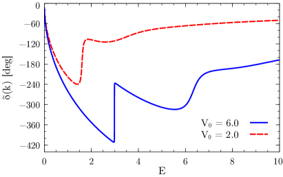
Figure 1: $S$-wave phase shift of two particles interacting via the potential given in Eq. (34) as a function of the (dimensionless) relative kinetic energy $E$ for $V_{0}=6.0$ (blue solid curve) and $V_{0}=2.0$ (red dashed curve).

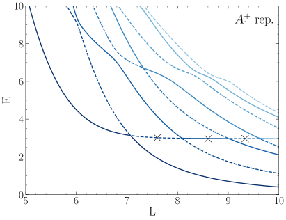
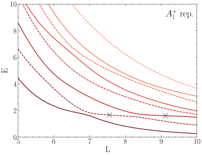
Figure 2: Energy spectrum of two particles interacting via the potential given in Eq. (34) in finite volume for different box sizes $L$. The left panel shows results for $V_{0}=6.0$ in the $A_{1}^{+}$ representation, whereas for the right panel a weaker barrier $V_{0}=2.0$ was used. All crossings are avoided because the spectrum is fully projected on states with the same quantum numbers. The crosses mark the inflection points used to extract the resonance energy (see text).

We now perform finite-volume calculations of two particles in a three-dimensional box with periodic boundary conditions using the DVR method discussed in Sec. II. As avoided level crossings corresponding to a resonance are only expected for states with the same quantum numbers, we project onto states that belong to a single irreducible representation $\Gamma$ of the cubic group (see Sec. II.1.4) and definite parity. Specifically, we consider here only $A_{1}^{+}$ states, which to a good approximation correspond to $S$-wave states in the infinite volume. As shown in Table 2, the next higher angular momentum contributing to $A_{1}^{+}$ is $l=4$, which can be safely neglected for low-energy states.

Our results are shown in Fig. 2. In the spectrum for $V_{0}=6.0$ (left panel of Fig. 2), a series of extremely sharp avoided level crossings, forming an essentially horizontal plateau, is observed at approximately $E\approx 3.0$. According to Ref. Wiese (1989) the width of the resonance is related to the spacing of the different levels at the avoided crossing. Therefore, we conclude that the resonance is very narrow, and find good qualitative agreement with the parameters extracted from the phase shift. For the weaker potential ($V_{0}=2.0$, right panel of Fig. 2), on the other hand, the avoided level crossings are less sharp, pointing to a larger resonance width. Along with the observed sequence of plateaus at approximately $E=1.6$, we again find good qualitative agreement with the phase-shift calculation.

For a more definite analysis, we determine the inflection points of the level curves with a plateau shape and interpret these as an estimate for the resonance energy. For this extraction, we fit the coefficients $\{c_{i}\}$ of a polynomial,

$$E(L)=\sum_{i=0}^{i_{\text{max}}}c_{i}L^{i}\,,$$ (36)

to the plateau region of each curve in Fig. 2 and take the position of the plateau inflection point as the resonance energy. In the plots, we indicate these points with crosses. We vary the number of data points taken into account for the fit by adjusting the lower and upper boundary of the fit interval. Furthermore, we vary $i_{\text{max}}$ in Eq. (36) until we find the extracted resonance energy to be independent of the order of the polynomial. For $V_{0}=6.0$ and $V_{0}=2.0$ we obtain, respectively, $E_{R}=2.98(3)$ and $E_{R}=1.63(3)$, where the quoted errors correspond to the spread of the extracted inflection points from different plateau curves. This means that with the inflection-point method we obtain very good agreement with the resonance positions from the phase-shift determination, which justifies the use of this method for the resonance-energy extraction.

At higher energies the spectra for both $V_{0}=6.0$ and $V_{0}=2.0$ exhibit less pronounced avoided level crossings. These structures, however, do not show clear plateaus, instead varying strongly as a function of the box size. Most likely these finite-volume features correspond to the resonancelike jumps of the phase shift at $E\sim 6-10$ for $V_{0}=6.0$ and $E\sim 3-7$ for $V_{0}=2.0$, respectively, which may correspond to broader resonances.

Altogether, we have demonstrated here that the positions of narrow two-body resonances can be extracted from finite-volume calculations with very good quantitative agreement compared to other methods.

IV Applications to three and four particles

We now proceed to explore the method in the three- and four-body sector, starting with bosonic (spin-0) particles. Because these lack a spin degree of freedom, we can quite easily achieve large DVR basis dimensions for these systems, whereas fermionic systems are more computationally demanding.

IV.1 Three-body benchmark

To verify our hypothesis that, analogously to the two-body case, three-particle resonances appear as avoided level crossings in finite-volume spectra, we start with three identical spin-0 bosons with mass $m=939.0\leavevmode\nobreak\ \mathrm{MeV}$ (mimicking nucleons) interacting via the two-body potential,

$$V(r)=V_{0}\exp\biggl{(}-\Bigl{(}\frac{r}{R_{0}}\Bigr{)}^{2}\biggr{)}+V_{1}\exp\biggl{(}-\Bigl{(}\frac{r-a}{R_{1}}\Bigr{)}^{2}\biggr{)}\,,$$ (37)

where $V_{0}=-55\leavevmode\nobreak\ \mathrm{MeV}$, $V_{1}=1.5\leavevmode\nobreak\ \mathrm{MeV}$, $R_{0}=\sqrt{5}\leavevmode\nobreak\ \mathrm{fm}$, $R_{1}=10\leavevmode\nobreak\ \mathrm{fm}$, and $a=5\leavevmode\nobreak\ \mathrm{fm}$. This setup was studied in Ref. Fedorov et al. (2003), where Faddeev equations with complex scaling were used to calculate resonances, as well as in Ref. Blandon et al. (2007), which used slow-variable discretization to extract three-body resonance parameters. The potential given in Eq. (37) supports a two-body bound state (dimer) at $E=-6.76\leavevmode\nobreak\ \mathrm{MeV}$ Fedorov et al. (2003) and a three-boson bound state at $E=-37.35\leavevmode\nobreak\ \mathrm{MeV}$ Blandon et al. (2007) (Ref. Fedorov et al. (2003) obtained $E=-37.22\leavevmode\nobreak\ \mathrm{MeV}$ for this state). In addition, it was found that there is a three-boson resonance at $E_{R}=-5.31\leavevmode\nobreak\ \mathrm{MeV}$ with a half width of $0.12\leavevmode\nobreak\ \mathrm{MeV}$ Blandon et al. (2007) ($E_{R}=-5.96\leavevmode\nobreak\ \mathrm{MeV}$ and $\Gamma/2=0.40\leavevmode\nobreak\ \mathrm{MeV}$ according to Ref. Fedorov et al. (2003)), which decays into a dimer-particle state that is overall lower in energy.

Using Eq. (37) with our DVR method, we find $E=-6.756(1)$ and $E=-37.30(5)$ for two and three bosons, respectively, in good agreement with the results of Refs. Blandon et al. (2007); Fedorov et al. (2003). Note that bound-state energies converge exponentially to the physical infinite-volume values as we increase the box size $L$ (see, e.g., Refs. König and Lee (2018); Meißner et al. (2015)). In order to look for the three-boson resonance, we study the positive-parity three-body spectrum as a function of $L$. For small box sizes around $L\sim 20\leavevmode\nobreak\ \mathrm{fm}$, we find that $N=26$ DVR points is sufficient to obtain converged results. For large box size ($L\sim 40\leavevmode\nobreak\ \mathrm{fm}$), on the other hand, we performed calculations using $N=30$. The terms “small” and “large” here refer to the scale set by the range of the interaction, which is quite sizable for the parameters given below Eq. (37).

Our combined results are shown in Fig. 3, where we also indicate the irreducible representations of the energy levels shown. These assignments were determined by running a set of cubic-projected calculations at small volumes. The levels corresponding to $A_{1}^{+}$ clearly show an avoided crossing at about the expected resonance energy from Ref. Blandon et al. (2007), which is indicated in Fig. 3 as a shaded horizontal band, the width of which corresponds to $E_{R}\pm\Gamma/2$. For the other states (with quantum numbers $E^{+}$ and $T_{2}^{+}$) shown in the figure we do not observe avoided crossings or plateaus. At $L\sim 38\leavevmode\nobreak\ \mathrm{fm}$ there is an actual crossing between $A_{1}^{+}$ and an $E^{+}$ levels. This is not a very sharp avoided crossing because the participating levels belong to different cubic representations.

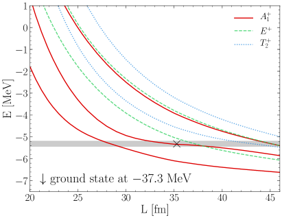
Figure 3: Energy spectrum of three bosons in finite volume for different box sizes $L$ interacting via the potential given in Eq. (37). States corresponding to the irreducible representation $A_{1}$ of the cubic symmetry group are shown as solid lines, whereas $E^{+}$ and $T_{2}^{+}$ states are indicated as dashed and dotted lines, respectively. The shaded area indicates the resonance position and width as calculated in Ref. Blandon et al. (2007), whereas the cross marks the inflection point used here to extract the resonance energy (see text).

To extract the resonance energy from the spectrum shown in Fig. 3 we proceed as described in Sec. III and extract the inflection points of the curves corresponding to the $A_{1}^{+}$ states by fitting polynomials. For the first excited state we find the fit to be quite sensitive to the number of data points included in the fit, which reflects the fact that this level does not exhibit a pronounced plateau. For the second excited state, however, there is a clearly visible plateau. Applying our fit method to this state, we extract a resonance energy $E_{R}=-5.32(1)\leavevmode\nobreak\ \mathrm{MeV}$. This means that within the quoted uncertainty, determined by varying the number of data points included in the fit as well as the order of the fit polynomial, we obtain good agreement with the resonance energy obtained in Ref. Blandon et al. (2007). While a determination of the resonance width is left for future work, we conclude from this result that indeed finite-volume spectra can be used to reliably determine the existence and energy of few-body resonances.

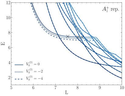
Figure 4: Energy spectrum of three bosons in finite volume for different box sizes $L$. The solid lines shows the spectrum for three bosons interacting purely via the shifted Gaussian potential given in Eq. (34) with $V_{0}=6.0$ while the dashed and dotted lines show results with an additional attractive three-body force as in Eq. (38). With increasing three-body force, the avoided level crossing is shifted to lower energy, while the rest of the spectrum remains unaffected. For each choice of the three-body force, all crossings are avoided because the spectrum is fully projected on states with the same quantum numbers. The crosses mark the inflection points used to extract the resonance energy (see text).

IV.2 Shifted Gaussian potentials

IV.2.1 Three bosons

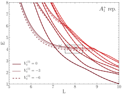
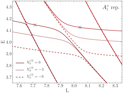
Figure 5: Energy spectrum of three bosons in finite volume for different box sizes $L$. The solid line shows the spectrum for three bosons interacting purely via the shifted Gaussian potential given in Eq. (34) with $V_{0}=2.0$ while the dashed and dotted lines show results with an additional attractive three-body force as in Eq. (38). With increasing three-body force the avoided level crossing is shifted to lower energy, while the rest of the spectrum remains unaffected. The dashed rectangle in the left panel indicates the zoomed region shown in the right panel. For each choice of the three-body force, all crossings are avoided because the spectrum is fully projected on states with the same quantum numbers. The crosses mark the inflection points used to extract the resonance energy (see text).

Having established the validity of the finite-volume method to extract three-body resonances, we now go back to the shifted Gaussian potential given in Eq. (34) which was used in Sec. III to study two-body resonances. Starting again with the stronger barrier, ($V_{0}=6.0$), we consider the $A_{1}^{+}$ spectrum for three bosons, calculated with $N=10$ DVR points and shown in Fig. 4 as solid lines. We observe a large number of avoided crossings at $E\sim 7.4$ as the box size $L$ is varied, producing together an almost horizontal plateau region. Using the same inflection-point method as discussed above, we extract $E=7.42(6)$ as a potential resonance energy. In addition to this, there are several avoided crossings at lower energies that have a significant slope with respect to changes in the box size, which we interpret as two-body resonances (known from Sec. III to exist at $E_{R}\sim 3.0$ for this potential) embedded into the three-body spectrum. To test this hypothesis we repeat the calculation with an added short-range three-body force,

$$V_{3}(x_{1},x_{2},x_{12})=V_{0}^{(3)}\exp\Biggl{(}{-}\biggl{(}\frac{x_{1}}{R_{0}^{(3)}}\biggr{)}^{2}\Biggr{)}\\ \hbox{}\times\exp\Biggl{(}-\biggl{(}\frac{x_{2}}{R_{0}^{(3)}}\biggr{)}^{2}\Biggr{)}\exp\Biggl{(}{-}\biggl{(}\frac{x_{12}}{R_{0}^{(3)}}\biggr{)}^{2}\Biggr{)}\,,$$ (38)

where $x_{12}=|\mathbf{x}_{1}-\mathbf{x}_{2}|$ and $R_{0}^{(3)}=1.0$ and varying strength $V_{0}^{(3)}$. Choosing a set of negative values for $V_{0}^{(3)}$ we find in Fig. 4 that the lower avoided crossings (and in fact most of the $L$-dependent spectrum) remain unaffected, whereas the upper plateau set is moved downwards as $V_{0}^{(3)}$ is made more negative.

Since the range $R_{0}^{(3)}=1.0$ was chosen small (compared to the box sizes considered), we expect it to primarily affect states that are localized in the sense that their wave function is confined to a relatively small region in the finite volume. Interpreting a resonance as a nearly bound state, its wave function should satisfy this criterion in the finite volume. On the other hand, scattering states or states where only two particles are bound or resonant are expected to have a large spatial extent. Based on this intuitive picture, we interpret the action of the three-body force as confirmation that indeed we have a genuine (because the potential we used does not support any bound states) three-boson resonance state at $E=7.42(6)$.

Similar to the two-body spectrum shown in the left panel of Fig. 2 we find that Eq. (34) with $V_{0}=6.0$ generates very sharp features in the three-boson spectrum so that even though we used a fine $L$ grid to generate Fig. 4 it is difficult to exclude that some crossings might not actually be avoided crossings. However, we observe the exact same qualitative behavior for the potential given in Eq. (34) with $V_{0}=2.0$, only that in this case the avoided crossings are broader and easily identified. From the spectrum, shown in Fig. 5, we extract $E=4.18(8)$ as the three-boson resonance energy for this case.

IV.2.2 Four bosons

Looking next at four bosons, we find a very similar picture. As shown in Fig. 6 for the shifted Gaussian potential given in Eq. (34) with $V_{0}=2.0$, the $L$-dependent $A_{1}^{+}$ four-boson spectrum (calculated with $N=8$ DVR points in this case) shows a large number of avoided level crossings that give rise to plateaus with different slopes. Interpreting the nearly horizontal set of avoided crossings as a possible four-boson resonance, we extract its energy as $E=7.26(2)$ with the inflection-point method. The more tilted sets of avoided crossings at lower energies most likely correspond to two- and three-boson resonance states embedded in the four-boson spectrum.

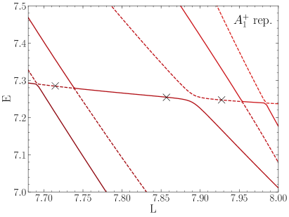
Figure 6: Energy spectrum of four bosons in finite volume for different box sizes $L$ interacting via the shifted Gaussian potential given in Eq. (34) with $V_{0}=2.0$. The dashed rectangle in the left panel indicates the zoomed region shown in the right panel. All crossings are avoided because the spectrum is fully projected on states with the same quantum numbers. The crosses mark the inflection points used to extract the resonance energy (see text).

IV.2.3 Three fermions

To conclude our survey, we now turn to fermionic systems. As the additional spin degree of freedom (we consider here identical spin-$1/2$ particles) increases the DVR basis size [see discussion below Eq. (13)], these calculations are more computationally demanding, but we can still achieve well-converged results for the shifted Gaussian potential given in Eq. (34). Before we turn to the three-body sector, we note that the results of Sec. III remain correct when we assume the two fermions to be in the channel with total spin $S=0$. In this case, the spin part of the wave function is antisymmetric and the spatial part has to be even under exchange. Because the latter corresponds to the bosonic case with positive parity, we conclude that for two spin-$1/2$ fermions the two-body potential given in Eq. (34) has a resonance state at $E_{R}\sim 1.6$ for $V_{0}=2.0$.

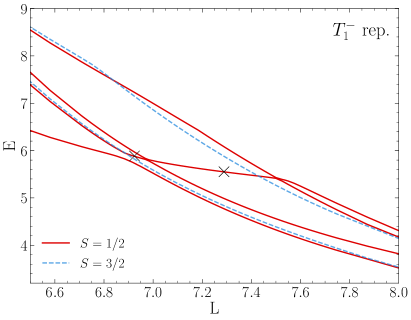
Figure 7: Negative-parity energy spectrum of three fermions in finite volume for different box sizes $L$ interacting via the shifted Gaussian potential given in Eq. (34) with $V_{0}=2.0$. All levels shown in the plot were found to belong to the $T_{1}^{-}$ cubic representation by performing fully projected calculations at selected volumes. Results are shown in the spin $S=1/2$ and $S=3/2$ channels. The crosses mark the inflection points used to extract the resonance energy (see text).

For three fermions, on the other hand, the situation is more involved because the overall antisymmetry of the wave function can be realized via different combinations of spin and spatial parts. Indeed, we find the finite-volume spectrum to look different from the bosonic case. For negative parity, we find the six lowest levels, shown in Fig. 7, to all belong to the $T_{1}^{-}$ cubic representation, which in this case we determined by running calculations with full cubic projections at selected volumes while otherwise only restricting the overall parity. Because the interaction we consider here is spin independent, total angular momentum $l$ and spin $S$ are separately good quantum numbers in infinite volume, and in the finite volume we likewise have $\Gamma$ and $S$ as good quantum numbers. The latter, which can be $S=1/2$ or $S=3/2$ for three spin-$1/2$ fermions, we determine by running calculations with fixed spin $z$-component at selected volumes, which can be realized by restricting the set of DVR basis states. Because $S=3/2$ states show up with both $S_{z}=3/2$ and $S_{z}=1/2$, whereas $S=1/2$ states are absent for $S_{z}=3/2$, we infer that four of the six levels shown in Fig. 7 have $S=1/2$, whereas the other two (given by the dashed lines in Fig. 7) have $S=3/2$.

For $S=1/2$ we observe a sequence of three avoided level crossings. Within this sequence there is a drift towards lower energies as $L$ increases, the magnitude of which is comparable to what we observe also for the three-boson spectra analyzed in Sec. IV.2.1 for the state that we concluded to correspond to an actual three-body resonance (based on varying the three-body force). We thus conclude that this effect is likely a residual volume dependence of an actual resonance state also in this case. With this interpretation, we extract a resonance energy $E_{R}=5.7(2)$ from the spectrum shown in Fig. 7 with our inflection-point method.

V Summary and outlook

We established the method of analyzing few-body energy spectra in finite periodic boxes to extract three- and four-particle resonance energies. Our approach relies on the observation of avoided level crossings and/or plateaus in the spectra considered as a function of the box size. Observing such features in few-body spectra and showing that they can be used to find and analyze resonance states, thus generalizing the method introduced in Ref. Wiese (1989) for two-body systems, is the central result of this work.

To calculate the finite-volume spectra, which were then used for the resonance identification, we used a DVR basis based on plane-wave states in relative coordinates. Resonance features are expected for finite-volume energies corresponding to scattering states in infinite volume. Unlike bound states, the energies of which converge exponentially with the box size $L$, finite-volume scattering states have a power-law dependence on $L$ (away from regions with avoided crossing). Looking at low-energy resonances therefore requires going to volumes that are sufficiently large for the relevant levels to come down to the energy range of interest. Because calculations in this regime typically require large DVR basis sizes and become computationally very demanding, we have developed a numerical framework to run the calculations on high-performance computing clusters when necessary. We have furthermore extended the formalism to include the symmetrization (antisymmetrization) to study bosonic (fermionic) systems, as well as for projecting onto the subspaces belonging to parity eigenstates and to the different irreducible representations of the cubic symmetry group. The latter allows us to determine the finite-volume quantum numbers of the resonance states that we find.

After testing our method in the two-body sector, where we verified the existence of resonances by looking at characteristic jumps in the scattering phase shifts as well as by looking for $S$-matrix poles on the second energy sheet, we studied three- and four-body systems with different potentials. First, we used a model potential known to generate a three-boson resonance that decays into a lower lying two-body bound state and a free particle. For this system, the resonance parameters were extracted previously based on different methods Blandon et al. (2007); Fedorov et al. (2003). Our results clearly show an avoided level crossing in the corresponding finite-volume spectrum and we find good agreement with the resonance energy of Ref. Blandon et al. (2007), which we extracted from the inflection points of the volume-dependent energy levels.

Taking this agreement as confirmation that our method works both qualitatively and quantitatively, we used shifted Gaussian potentials (with the same parameters known to generate two-body resonances) in the three- and four-body sector. Studying the three-boson finite-volume spectrum, we showed that an additional short-range three-body force can be used to move avoided crossings forming a plateau region whereas other avoided crossings remain unchanged. We interpret this as confirmation that the observed plateau region indeed corresponds to a three-body resonance (with a spatially localized wave function so that it “feels” the three-body forces), whereas the other levels likely correspond to two-body resonances plus a third particle. For the same shifted Gaussian potential we were also able to observe avoided crossings for three fermions and four bosons, from which we extracted resonance energies via the inflection-point method. Based on these findings, we conclude that our method can be used to search for possible three- and four-neutron resonances in future work.

Appendix A Cubic symmetry group

In this section, we briefly discuss how the projector on the irreducible representations of the cubic symmetry group in Eq. (31) is constructed. For each element of the cubic group $R\in\mathcal{O}$, the realization $D_{n}(R)$ used in Eq. (31) is given by a permutation and/or inversion of the components $c=1,2,3$ of each relative coordinate $\mathbf{x}_{i}$ (simultaneously for all $i=1,\ldots,n-1$).

Index	Class	$D_{n}(R)$			Index	Class	$D_{n}(R)$
1	$I$	$1$	$2$	$3$	13	$6C_{4}$	$2$	${-}1$	3
2	$3C_{2}$	${-}1$	${-}2$	$3$	14		${-}2$	1	3
3		${-}1$	$2$	${-}3$	15		$3$	$2$	${-}1$
4		$1$	${-}2$	${-}3$	16		${-}3$	$2$	$1$
5	$8C_{3}$	$3$	$1$	$2$	17		$1$	${-}3$	$2$
6		$2$	$3$	$1$	18		$1$	$3$	${-}2$
7		${-}2$	$3$	${-}1$	19	$6C_{2}^{\prime}$	$2$	$1$	${-}3$
8		${-}3$	${-}1$	$2$	20		${-}2$	${-}1$	${-}3$
9		$2$	${-}3$	${-}1$	21		$3$	${-}2$	$1$
10		${-}3$	$1$	${-}2$	22		${-}3$	${-}2$	${-}1$
11		${-}2$	${-}3$	$1$	23		${-}1$	${-}3$	${-}2$
12		$3$	${-}1$	${-}2$	24		${-}1$	$3$	$2$

Table 1: Realization of the 24 cubic rotations acting on a coordinate tuple in symbolic notation (see text). The second column indicates the conjugacy class of the rotation.

$l$	$A^{+}_{1}$	$A^{+}_{2}$	$E^{+}$	$T^{+}_{1}$	$T^{+}_{2}$	$A^{-}_{1}$	$A^{-}_{2}$	$E^{-}$	$T^{-}_{1}$	$T^{-}_{2}$
$0$	1
$1$									1
$2$			1		1
$3$							1		1	1
$4$	1		1	1	1
$5$								1	2	1
$6$	1	1	1	1	2
$7$							1	1	2	2
$8$	1		2	2	2
$9$						1	1	1	3	2
$10$	1	1	2	2	3

Table 2: Decomposition of the irreducible representations of the rotational symmetry group $SO(3)$ into irreducible representations of the cubic symmetry group $\mathcal{O}$; reproduced in part from Ref. Dresselhaus (2002).

In Table 1 we show these operations, where the notation gives the result of operating on a tuple $(k_{i,1},k_{i,2},k_{i,3})$ in a short-hand form, e.g., the rotation with index 7 transforms a tuple to $(-k_{i,2},k_{i,3},-k_{i,1})$. It is understood that, as discussed in Sec. II.1.3, each transformed index $k_{i,c}$ is wrapped back into the interval ${-}N/2,\ldots,N/2-1$, if necessary.

Cubic symmetry commutes with parity as well as permutation symmetry, so for both bosonic and fermionic systems we end up with multiplets of the irreducible representations $\Gamma=A_{1}^{\pm}$, $A_{2}^{\pm}$, $E^{\pm}$, $T_{1}^{\pm}$, and $T_{2}^{\pm}$, where the superscript indicates the parity. As already mentioned above, the irreducible representation of the full rotational group $SO(3)$ is reducible with respect to the cubic group. A basis for the irreducible representation of $SO(3)$ is given by the angular momentum multiplets, i.e., spherical harmonics $Y_{lm}$, labeled by the angular momentum quantum number $l$ and its projection $m$. The numerical values in Table 2 yield the multiplicity of the cubic irreducible representations in the decomposition of a given angular momentum multiplet. $l=0$ and $l=1$ contribute only to $A^{+}_{1}$ and $T^{-}_{1}$, respectively, meaning that an $S$-wave state is mapped solely onto the single $A_{1}^{+}$ state, while a $P$-wave state maps onto the three $T^{-}_{1}$ states in finite volume. A $D$-wave state with its five projections $m=0,\pm 1,\pm 2$ is decomposed into the two $E^{+}$ and three $T_{2}^{+}$ states.

To conclude this section, we note that in the case of spin-dependent interactions, total angular momentum $J$ instead of $l$ is the relevant good quantum number in the infinite volume. For example, in the case of spin-$1/2$ fermions, one has to consider $SU(2)$ broken down to the double cover ${}^{2}\mathcal{O}$ of the cubic group, giving three additional irreducible representations that receive contributions from half-integer $J$ states. For details, see Ref. Johnson (1982).

References

- Kisamori et al. (2016) K. Kisamori, S. Shimoura, H. Miya, S. Michimasa, S. Ota, M. Assie, H. Baba, T. Baba, D. Beaumel, M. Dozono, et al., Phys. Rev. Lett. 116, 052501 (2016).
- (2) S. Paschalis et al., Report No. NP1406-SAMURAI19 .
- (3) K. Kisamori et al., Report No. NP1512-SAMURAI34 .
- (4) S. Shimoura et al., Report No. NP1512-SHARAQ10 .
- Witała and Glöckle (1999) H. Witała and W. Glöckle, Phys. Rev. C 60, 024002 (1999).
- Lazauskas and Carbonell (2005a) R. Lazauskas and J. Carbonell, Phys. Rev. C 71, 044004 (2005a).
- Lazauskas and Carbonell (2005b) R. Lazauskas and J. Carbonell, Phys. Rev. C 72, 034003 (2005b).
- Hiyama et al. (2016) E. Hiyama, R. Lazauskas, J. Carbonell, and M. Kamimura, Phys. Rev. C 93, 044004 (2016).
- Klos et al. (2016) P. Klos, J. E. Lynn, I. Tews, S. Gandolfi, A. Gezerlis, H. W. Hammer, M. Hoferichter, and A. Schwenk, Phys. Rev. C 94, 054005 (2016).
- Shirokov et al. (2016) A. M. Shirokov, G. Papadimitriou, A. I. Mazur, I. A. Mazur, R. Roth, and J. P. Vary, Phys. Rev. Lett. 117, 182502 (2016).
- Gandolfi et al. (2017) S. Gandolfi, H.-W. Hammer, P. Klos, J. E. Lynn, and A. Schwenk, Phys. Rev. Lett. 118, 232501 (2017).
- Fossez et al. (2017) K. Fossez, J. Rotureau, N. Michel, and M. Płoszajczak, Phys. Rev. Lett. 119, 032501 (2017).
- (13) A. Deltuva, Phys. Rev. C 97, 034001 (2018).
- Lüscher (1986) M. Lüscher, Commun. Math. Phys. 105, 153 (1986).
- Lüscher (1991) M. Lüscher, Nucl. Phys. B 354, 531 (1991).
- Beane et al. (2011) S. R. Beane, W. Detmold, K. Orginos, and M. J. Savage, Prog. Part. Nucl. Phys. 66, 1 (2011).
- Briceno et al. (2018) R. A. Briceno, J. J. Dudek, and R. D. Young, Rev. Mod. Phys. 90, 025001 (2018).
- Beane et al. (2004) S. R. Beane, P. F. Bedaque, A. Parreño, and M. J. Savage, Phys. Lett. B 585, 106 (2004).
- Kreuzer and Hammer (2011) S. Kreuzer and H.-W. Hammer, Phys. Lett. B 694, 424 (2011).
- Polejaeva and Rusetsky (2012) K. Polejaeva and A. Rusetsky, Eur. Phys. J. A 48, 67 (2012).
- Hansen and Sharpe (2015) M. T. Hansen and S. R. Sharpe, Phys. Rev. D 92, 114509 (2015).
- Briceno and Davoudi (2013) R. A. Briceno and Z. Davoudi, Phys. Rev. D 87, 094507 (2013).
- Hammer et al. (2017) H.-W. Hammer, J.-Y. Pang, and A. Rusetsky, JHEP 09 (2017), 109.
- König and Lee (2018) S. König and D. Lee, Phys. Lett. B 779, 9 (2018).
- Mai and Döring (2017) M. Mai and M. Döring, Eur. Phys. J. A 53, 240 (2017).
- Wiese (1989) U. J. Wiese, Nucl. Phys. Proc. Suppl. 9, 609 (1989).
- Maier et al. (1980) C. H. Maier, L. S. Cederbaum, and W. Domcke, J. Phys. B 13, L119 (1980).
- Fedorov et al. (2009) D. V. Fedorov, A. S. Jensen, M. Thogersen, E. Garrido, and R. de Diego, Few Body Syst. 45, 191 (2009).
- Meißner et al. (2015) Ulf-G. Meißner, G. Ríos, and A. Rusetsky, Phys. Rev. Lett. 114, 091602 (2015).
- Bulgac and Forbes (2013) A. Bulgac and M. McNeil Forbes, Phys. Rev. C 87, 051301 (2013).
- Groenenboom (2001) G. C. Groenenboom, www.theochem.kun.nl/~gerritg.
- Bilaj (2017) S. Bilaj, Bachelor’s thesis, TU Darmstadt, 2017.
- Varga and Suzuki (1997) K. Varga and Y. Suzuki, Comput. Phys. Commun. 106, 157 (1997).
- Johnson (1982) R. C. Johnson, Phys. Lett. B 114, 147 (1982).
- Intel® (a) Computer code TBB, Threading Building Blocks, www.threadingbuildingblocks.org (Intel, Santa Clara, 2017) .
- (36) K. J. Maschhoff and D. C. Sorensen, P_ARPACK: An Efficient Portable Large Scale Eigenvalue Package for Distributed Memory Parallel Architectures, www.caam.rice.edu/software/ARPACK/, https://github.com/opencollab/arpack-ng.
- Intel® (b) Computer code MKL, Math Kernel Library, https://software.intel.com/mkl (Intel, Santa Clara, 2017).
- (38) M. Martone, librsb: A shared memory parallel sparse matrix computations library for the Recursive Sparse Blocks format, www.librsb.sourceforge.net.
- Frigo and Johnson (2005) M. Frigo and S. G. Johnson, Proc. IEEE 93, 216 (2005).
- Glöckle (1983) W. Glöckle, The Quantum Mechanical Few-Body Problem (Springer-Verlag, Berlin, 1983).
- Fedorov et al. (2003) D. V. Fedorov, E. Garrido, and A. S. Jensen, Few-Body Syst. 33, 153 (2003).
- Blandon et al. (2007) J. Blandon, V. Kokoouline, and F. Masnou-Seeuws, Phys. Rev. A 75, 042508 (2007).
- Dresselhaus (2002) M. S. Dresselhaus, Application of Group Theory to Physics of Solids, http://web.mit.edu/course/6/6.734j/www/group-full02.pdf (Massachusetts Institute of Technology, Cambridge, 2002).