Understanding doped perovskite ferroelectrics with defective dipole model

Abstract

While doping is widely used for tuning physical properties of perovskites in experiments, it remains a challenge to exactly know how doping achieves the desired effects. Here, we propose an empirical and computationally tractable model to understand the effects of doping with Fe-doped BaTiO₃ as an example. This model assumes that the lattice sites occupied by Fe ion and its nearest six neighbors lose their ability to polarize, giving rise to a small cluster of defective dipoles. Employing this model in Monte-Carlo simulations, many important features like reduced polarization and the convergence of phase transition temperatures, which have been observed experimentally in acceptor doped systems, are successfully obtained. Based on microscopic information of dipole configurations, we provide insights into the driving forces behind doping effects and propose that active dipoles, which exist in proximity to the defective dipoles, can account for experimentally observed phenomena. Close attention to these dipoles are necessary to understand and predict doping effects.

I Introduction

For perovskite ferroelectrics, doping chemical elements is an important way to improve or modify their properties and performances (Jung, ; Yang, ; Shi, ; Limpichaipanit, ). In many cases, it appears that minuscule doping already have strong effects on the resulting materials. While there is a large amount of literature on exploiting doping effects experimentally, the nature and cause of the observed effects are not fully understood, and several possible factors are proposed to explain experimental results. The effects of doping induced oxygen vacancies and ferroelectric domains, among others, are often believed to play important roles (Ang, ; Renxb, ; Deng, ; Zhang_Mn, ; Hong, ; Jin, ; Jin_2, ; Gao, ; Chapman, ; Liu, ). In fact, the exact mechanism of doping effects is hard to identify by working backward (i.e., to deduce directly from experimental results), thus a lot of theoretical modeling is needed in this process. Usually, the most reliable method to calculating doping effect is the first principle calculation. However, this method has practical difficulty for minisacle doping where too many atoms are needed in the simulations, which causes heavy computational burden. Here we focus on the iron doping BaTiO₃ and consider this problem in an opposite direction (generative, ). In other words, we first propose a computationally tractable model regarding how doping works, and then with the effective Hamiltonian approach (Zhong, ; Wang_2014, ; Al-Barakaty, ; Wang-1, ), we explore the consequences of the proposed model. Comparing the simulated results for samples with and without doping to experimental results, one will gain better understanding of the nature of doping effects.

Barium titanate (BaTiO₃), a typical ferroelectric oxide with perovskite ABO₃ structure (with Ba on the A site and Ti on the B site), has been widely investigated due to its high dielectric permittivity, excellent electrical properties, and environmental friendliness(Senn2016, ; Qi, ). Doping of BaTiO₃-based materials with different chemical elements has been an attractive topic of research (Yu_z, ; West, ; Xu, ; Hennings1982, ; Jin2016, ; Yasmm, ), with the goal to improve material performance. One important line of research is to dope rare earth elements in BaTiO₃. For instance, Yasmin et al. found that the Ce-doped BaTiO₃ has a dielectric permittivity as high as 2050 and a decreased Curie temperature, $T_{C}=313$ K(Yasmm, ). Ganguly et al. reported that at 10 kHz, the dielectric permittivity for (Ba_1-xLa_2x/3)TiO₃ ($x=0.1$) can reach 10400 at $T_{C}\simeq 168$ K (Ganguly, ). Ba(Zr_xTi_1-x)O₃ ceramics, where the B-site Ti is substituted with Zr, shows enhanced remnant polarization and field piezoelectric strain coefficient $d_{33}$(Yu_z, ), as well as interesting dielectric properties on the subterahertz frequency range (Wang-1, ). La and Zr co-doped BaTiO₃ can obtain a dielectric permittivity as high as 36000 (West, ). In addition, doping transitional metal ions could also achieve novel ferromagnetic properties with a saturation magnetization value as large as 0.012 emu/g (Xu, ; Chakraborty, ).

In experimental investigations of doped systems, three phenomena are often observed as the consequences of doping: (i) Strong change of the hysteresis loop; (ii) Diffused and/or smeared dielectric permittivity with respect to temperature; (iii) Variations of phase transition temperatures (Xu, ; Hennings1982, ; Weber, ; Baskaran, ; Wang, ; Nanakorn, ; Kundu, ; Leontsev, ; Guo, ; Huang_0.8, ). Moreover, it is also known from experiments that doping Fe or Mn into BaTiO₃ in general makes ferroelectric materials easier to reverse (Haertling_1999, ; Chen, ; Tangsritrakul, ; Khirade, ). Since the doping effects can be significant even with minuscule doping, the origin of such effects naturally attracts great scientific attention. Different explanations have been proposed to understand the mechanism of doping effects, including (i) Oxygen vacancies and free charges on the doped lattice point(Jin, ; Gao, ; Chapman, ; Liu, ; Tangsritrakul, ; Shuai, ; scott, ); (ii) Local strains (Choi, ; Wu, ; Xu_AFM, ); (iii) Domains induced by dopants (Hong, ; Jin, ; Jin_2, ; Wada, ). In the present work, we propose a computationally tractable model where the dipoles associated with Fe-doped lattice sites and their nearest neighbors are suppressed. We apply this model to mimic Fe-doped BaTiO₃ and perform first-principles-based Monte-Carlo (MC) simulations, showing that the simulated results can account for many experimentally observed phenomena. Through the aforementioned approach, we hope to better understand the most important factors that determine properties of BaTiO₃ doped with iron.

This paper is organized as follows. In Sec. II, we introduce the defective dipole model and the effective Hamiltonian method for numerical simulation. In Sec. III and Sec. IV, we apply this model to samples mimicking Fe-doped BaTiO₃ and numerically obtain the results of doping. In Sec. V, we propose the concept of active dipoles and use it (along with dipole distributions) to explain doping effects. Finally, in Sec. VI, we present a brief conclusion.

II Method

The transition metal ions we are concerned with, including Fe, Mn and Co, have one or more vacant orbitals (e.g., d-orbitals) that may host extra electrons. Their electronic properties need a large on-site energy $U$ to be properly understood (Leontsev, ; Chen, ; Anderson, ; Hubbard, ). When extra charge carriers are (temporarily) captured by these ions, the localized charges can: (i) distort local electronic band structure and (ii) introduce extra Coulomb interaction between neighboring sites. For instance, it was estimated that the interaction energy between two localized electrons on nearest neighbors can be as large as 2-3 eV (Hubbard, ). Therefore, it is conceivable that around the dopants, this type of interaction may strongly affect the dipoles (arising from displacements of ions) that exist on each unit cell of ferroelectric materials.

In addition, depending on the impurity energy $\varepsilon_{d}$ (relative to the Fermi level), the local conductivity could be changed [related to the aforementioned effect (i)] (Patino, ). If the local conductivity is high, local dipoles cannot exist because the electric field associated with dipoles will lead to the redistribution of charge carriers and eventually neutralize the bound charges induced by displacements of ions, which are responsible for forming the dipoles in the first place.

Based on the above arguments we propose that dipoles on and around the Fe sites are suppressed and remain constant. Thus, the number of suppressed dipole should be equals to 7 times of the doped iron. The precise number could be calculated by the equation $n_{\textrm{dipole}}=7\times n_{\textrm{Fe}}$, which is is always satisfied, until two or more defective dipoles contact with each other. In addition, while we aim at Fe doped BaTiO₃, it is likely that similar arguments can be used for other transitional metal (Zhang_Mn, ; Chen, ; Ihrig, ; Ihrig_valence, ). However, the exact number of defective dipoles induced by one dopant should be determined empirically.

We use effective Hamiltonian based MC simulations to obtain finite temperature properties. A pseudo-cubic supercell of size $\mathrm{12\times 12\times 12}$ (i.e., 1728 unit cells, 8640 atoms) with periodic boundary conditions is employed in simulations. Among all the unit cells, we randomly select a certain number of them to represent Fe ion doped cells. The dipole moments on these selected sites are set to null in MC simulations. In addition, due to the influence of the Fe dopants, all its six first nearest neighbors are set to be defective too. The total energy is given by the effective Hamiltonian developed in Ref. [Zhong, ]:

$$E^{\textrm{tot}} =E^{\textrm{self}}\left(\left\{\boldsymbol{u}\right\}\right)+E^{\textrm{dpl}}\left(\left\{\boldsymbol{u}\right\}\right)+E^{\textrm{short}}\left(\left\{\boldsymbol{u}\right\}\right)$$

$$+E^{\textrm{elas}}\left(\left\{\eta_{l}\right\},\eta_{H}\right)+E^{\textrm{int}}\left(\left\{\boldsymbol{u}\right\},\left\{\eta_{l}\right\},\eta_{H}\right)$$ (1)

which consists of five parts: (i) the local-mode self-energy, $E^{\textrm{self}}\left(\left\{\boldsymbol{u}\right\}\right)$; (ii) the long-range dipole-dipole interaction, $E^{\textrm{dpl}}\left(\left\{\boldsymbol{u}\right\}\right)$; (iii) the short-range interaction between soft modes, $E^{\textrm{short}}\left(\left\{\boldsymbol{u}\right\}\right)$; (iv) the elastic energy, $E^{\textrm{elas}}\left(\left\{\eta_{l}\right\}\right)$; (v) the interaction between the local modes and local strain, $E^{\textrm{int}}\left(\left\{\boldsymbol{u}\right\},\left\{\eta_{l}\right\}\right)$, where $\boldsymbol{u}$ is the local soft-mode amplitude vector (directly proportional to the local polarization) and $\eta_{H}$ ($\eta_{l}$) is the six-component homogeneous (inhomogeneous) strain tensor in Voigt notation (Zhong, ). The parameters appearing in the effective Hamiltonian have been reported in Ref. [Nishimatsu, ].

In order to understand the doping effects, we build samples of different dopant concentrations from $0\,\%$ to $2\,\%$, with an increasing step of 0.2 %. For each of the doped samples, we gradually cool down the system from high (typically 550 K) down to low (typically 30 K) temperatures with a step of 10 K. For each temperature, we typically carry out 320,000 steps of MC. The first 160,000 steps are used to equilibrate the system, and the remaining steps to obtain averaged quantities, e.g., supercell average of local mode. For doped BaTiO₃, with increasing dopant concentration, fluctuations close to phase transitions become so larger that more MC steps (e.g., 640,000) and/or large supercells (e.g., $18\times 18\times 18$) are used to obtain satisfactory results.

To analyze dipole distributions, we have also obtained snapshots of all the dipoles in the supercell, which are typically captured at the ending stage of MC simulations when dipoles do not change much. In addition, averaged dipole configurations are obtained by storing a snapshot of dipoles every 400 MC steps after the equilibration stage. We then use all the stored snapshots to calculate the averaged local dipole in each unit cell and perform statistics on theses dipoles.

Understanding the mechanism of doping has attracted much attention. Given the variety of doping, fully understanding how doping works is an immense task and, not surprisingly, different models had been proposed. In general, depending on the valence state of the dopant ions, acceptor doping can induce oxygen vacancies, while donor doping will induce A-site vacancy or conduction electrons (Deng, ; Ganguly, ). Understanding such complex systems from numerical simulation often requires a priori assumption and modeling about doping. Proposed mechanisms include: (i) Defective dipoles can be caused by dopants (which is the mechanism we employ in this work); (ii) Local strain can be induced due to the different ionic radius of the dopants (Chakraborty, ); (iii) As a result of oxygen vacancies and localized charges created by doping, new dipoles (defect dipoles) can be induced (Liu, ; XuBx, ; Shuai, ; scott, ); (iv) Dopants can affect the grain size and/or induce new domains in the matrix material (Hong, ; Jin, ; Jin_2, ; Wada, ; Murugaraj, ). Recently, Xu et al. show that antiparallel defect dipoles could induce a negative electrocaloric effect and double-peak behaviors for acceptor doped BaTiO₃(XuBx, ). Cohen and co-workers successfully simulated the pinched and shifted hysteresis loop and the large recoverable electromechanical response using defect dipoles (Chapman, ; Liu, ). However, due to the long range interaction of dipoles, the fixed dipoles seem to increase the phase temperature, which is not consistent with experimental results and verified by our simulations. Therefore, further refined models or other factors, such as the one discussed here, are needed.

III Doping effects

Having described our approach, we now use MC simulations to calculate basic properties of BaTiO₃ with different dopant concentration. We first obtain and show their hysteresis loops, polarizations, as well as phase transition temperatures, which are summarized to illustrate the trend of changes with respect to dopant concentration. With all simulation results, we are also able to obtain the phase diagram of Fe-doped BaTiO₃ with respect to temperature and dopant concentration. In this way, we show that the model can indeed generate important features of Fe-doped BaTiO₃ that are observed in experiments.

III.1 Hysteresis loop

Figure 1: (a)–(d) Electric hysteresis loops of doped BaTiO₃ are shown for various dopant concentration at 300 K.

Figure 1 shows the hysteresis loops of the doped BaTiO₃ at selected dopant concentrations ($p=0\,\%,$ $0.6\,\%$, $1.2\,\%$, and $1.8\,\%$) at 300 K. The motion of oxygen vacancies is not included, therefore we are not able to observe the aging phenomenon(Renxb, ; Zhang_Mn, ; Gao, ; Chapman, ; Liu, ; Huang_0.8, ). Figure 1(a) demonstrates a typical hysteresis loop of ferroelectric materials, with large coercive electric field $E_{c}$ (the electric field when polarization changes sign) and large remnant polarization $P_{r}$ (the remaining polarization when the electric field $E=0$ V/m), as well as large saturation polarization $P_{s}$ (the polarization at very large $E$). As $p$ increases, both $E_{c}$ and $P_{s}$ decrease. For $p\geq 1.2\,\%$, the hysteresis loop disappears completely [see Fig. 1 (c) and (d)], indicating some critical changes that will be further discussed in Sec. V.2. Such changes with respect to dopant concentration is perhaps the most notable phenomenon observed and reported in experimental work (Yu_z, ; Tangsritrakul, ; Khirade, ; Qiu, ; Dutta, ).

To quantitatively check the doping effects, in Fig. 2 we plot $P_{s}$ (polarization obtained at $E=6\times 10^{7}\,\textrm{V/m}$), $P_{r}$, and $E_{c}$ as functions of $p$, the dopant concentration. It can be seen that $P_{s}$ depends linearly on the concentration. According to our assumption, introducing a dopant ion will bring in seven dead dipoles near the defect sites. Therefore, at the dopant concentration $p$, the estimated saturation polarization should not exceed

$$P_{s}\left(p\right)\simeq P_{s}\left(0\right)\times\left(1-7p\right),$$ (2)

which is shown as the gray dashed line in Fig. 2. As a matter of fact, $P_{s}$ declines faster than this estimation, which indicates the importance of dipole correlations in ferroelectric materials. Figure 2 also shows that both $P_{r}$ and $E_{c}$ have a sudden change at some critical values of $p$ ($p\simeq 0.8\,\%$ and $p\simeq 1.2\,\%$), beyond which they become zero.

In order to compare to experimental results, we plot the simulation results of $P_{r}$ to that of Fe-doped 0.5Ba(Zr_0.2Ti_0.8)O₃-0.5(Ba_0.7Ca_0.3)TiO₃ (Jin2016, ) obtained experimentally in Fig. 2. The change of $P_{r}$ obtained from our simulations shows some interesting agreement with experiments (BCZT, ). We note that to the experimental data is normalized to compare with our simulation results. In this process, we use the polarization of the 0.25 % doped sample as unit (and set this value to that obtained from our simulation) to scale the values of others.

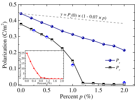
Figure 2: The saturation polarization, $P_{s}$, the remnant polarization $P_{r}$, and the coercive field, $E_{c}$ (inset) change with dopant concentration. (Normalized experimental data from Refs. [Jin2016, ] are shown as blue and white diamonds; see the text)

III.2 Phase transition

To reveal how doped BaTiO₃ evolves with temperature, we show the averaged components of the polarization$\left\langle\boldsymbol{P}\right\rangle$ in Fig. 3. For pure BaTiO₃ shown in Fig. 3(a), there exist four regions:

1. For $T>390$ K, no polarization exists in any direction (i.e., $\left\langle P_{x}\right\rangle=\left\langle P_{y}\right\rangle=\left\langle P_{z}\right\rangle=0$), showing a paraelectric phase (P);

2. For $200\,\textrm{K}<T<390$ K, $\left\langle P_{z}\right\rangle$ becomes nonzero ($0.3-0.42$ C/$m^{2}$), showing a tetragonal phase (T, space group $P4mm$);

3. For $90\,\textrm{K}<T<200$ K, $\left\langle P_{y}\right\rangle$ and and $\left\langle P_{z}\right\rangle$ equal to each other ($\sim 0.35$ C/$m^{2}$) while $\left\langle P_{x}\right\rangle$ is still zero, showing an orthorhombic phase (O, space group $Amm2$);

4. For $T<90$ K, the system reaches the rhombohedral phase (R, space group $R3m$) with $\left\langle P_{x}\right\rangle=\left\langle P_{y}\right\rangle=\left\langle P_{z}\right\rangle\simeq 0.3\thinspace\textrm{C/$m^{2}$}$.

We note that the above calculated results are consistent with previous experimental(Huang_0.8, ; Qiu, ) and theoretical results (Qi, ; Vielma, ; Nishimatsu, ), where the polarization being 0.33 (R), 0.36 (O), and 0.27 C/$m^{2}$ (T) (Qi, ) and the phase transition temperatures are $T_{2}\simeq 90$ K (O to R), $T_{1}\simeq 200$ K, (T to O) $T_{C}\simeq 390$ K (P to T)(Nishimatsu, ).

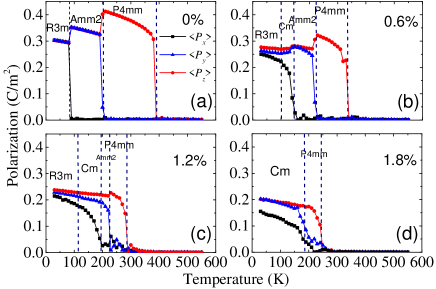
Figure 3: The polarization versus temperature are shown for selected dopant concentration. The dashed vertical lines show the separation between different phases.

For doped BaTiO₃, Fig. 3(b-d) show their phase transition temperatures and phase transition sequences. At $p=0.6\,\%$, all the phases appearing in pure BaTiO₃ can still be seen while the phase transition temperatures are different. On the other hand, when $p=1.2\,\%$, the P-T phase change happens at $T_{C}\simeq 285\,\textrm{K}$ and the T-O at $T_{1}\simeq 240\,\textrm{K}$, leaving a narrower region for the T phase. Finally, at $T_{2}=180\,\textrm{K}$, the system changes from the $Amm2$ phase (orthorhombic) to the $Cm$ phase (monoclinic, M). At $p=1.8\,\%$, the phase transitions become completely different with the $Cm$ phase appearing at the lowest temperatures. In general, it can be seen from Fig. 3 that $\left\langle\boldsymbol{P}\right\rangle$ decreases with $p$. In addition, for large $p$, we have to endure some ambiguity in determining the phase transition temperatures as the phase transition become diffused.

Figure 4: Phase transition temperatures are plotted against dopant concentration.

Doping effects on phase transitions can be summarized in the phase diagram shown in Fig. 4, which reveals that for Fe-doped BaTiO₃ with $p\leq 2.0\,\%$, four phases exist: (i) Between $T_{C}$ and $T_{1}$, the $P4mm$ phase; (ii) Between $T_{1}$ and $T_{2}$, the $Amm2$ phase; (iii) Below $T_{2}$, the $R3m$ or $Cm$ phase. The existence of the $R3m$ and the $Cm$ phase indicates a possible morphotropic boundary that is interesting for potential performance enhancement (boundary, ). We can also see, as $p$ increases, $T_{C}$ decreases quickly from 375 K (at $p=0.0\,\%$) to ~250 K (at $p=2.0\,\%$), resulting in a decreasing rate of 57 K/(1% doping). Such decreasing rate is much smaller for Mn (with experimental results being ~15 K/(1% doping) (Chen, ), and other similar elements (Ihrig, ; Ihrig_valence, ). On the other hand, $T_{2}$ increases from 85 K (at $p=0\,\%$) to ~250 K (at $p=2.0\,\%$). Moreover, the shift of $T_{1}$ is relatively small comparing to the other two. The convergence of $T_{C}$, $T_{1}$ and $T_{2}$ around $p\simeq 2.0\,\%$ agree very well with experimental results with doped BaTiO₃ (Ihrig, ) , which also slightly resembles what happens with Ba(Zr,Ti)O₃ when Zr concentration increases(Yu_z, ; Yu_BZT, ; Kuang_BZT, ). Both the variation trend and speed of character temperature will be further discussed in Sec. V.3.

IV Dipole distribution

In order to understand doping effects on macroscopic properties of BaTiO₃, we need to know how microscopic dipole configuration responds to doping. To this end, in this section we focus on orientation and magnitude distributions of dipoles in pure and doped BaTiO₃ to gain insights into how doping works.

IV.1 Orientation

Figure 5: Dipole orientation distribution calculated from dipole snapshot at 450 K, 300 K, 170 K, and 30 K. (a-d) Pure BaTiO₃; (e-h) Doped BaTiO₃ with $p=0.6\,\%$; (i) Dipole orientation distribution on a unit sphere.

In Fig. 5, the orientation distribution of dipoles for pure and $0.6\,\%$ doped BaTiO₃ are shown for selected temperatures (450, 300, 170, and 30 K). At each temperature, we categorize dipoles as $\left\langle 100\right\rangle$, $\left\langle 110\right\rangle$, or $\left\langle 111\right\rangle$ type dipoles, depending on their orientations. Figure 5(i) shows a schematic drawing of how the categorization is performed and Fig. 5 (a-h) show the number of dipoles in each category for pure BaTiO₃ at the selected temperatures.

Figure 5(a) shows that, at $T=450$ K (paraelectric phase), owing to the large thermal fluctuation, all three types have significant number of dipoles, with 20.2 % for $\left\langle 100\right\rangle$, 46.6 % for $\left\langle 110\right\rangle$, and $33.2\,\%$ for $\left\langle 111\right\rangle$. The 0.6 % doped BaTiO₃ [Fig. 5(e)] almost has the same distribution. Given such a distribution, at this temperature the averaged values (e.g. $\left\langle\boldsymbol{P}\right\rangle$) are very small (see Fig. 3), producing a paraelectric phase.

At $T=300$ K (macroscopic $P4mm$ phase), Fig. 5(b) shows that the number of $\left\langle 100\right\rangle$ dipoles have significantly increased, while the number in the other two categories decreased. Besides, snapshots of dipole configurations reveal that most dipoles ($>95\,\%$) has positive $z$ component for both pure and 0.6% doped BaTiO₃. This means that a preferred direction ($\left[001\right]$ here) has established at $300$ K in the system, likely due to the longe-range dipole-dipole interaction. At $T=170$ K [$Amm2$, see Fig. 5(c) and (g)], the averaged polarization $\left\langle\boldsymbol{P}\right\rangle$ is along the $\left[011\right]$ direction, consistent with experimental results. However, for a single snapshot, a large portion (~27 %) of dipoles belongs to the $\left\langle 111\right\rangle$ category. In addition, doping gives rise to more “disobedient” dipoles that do not follow the overall orientation. For instance, in pure BaTiO₃ 70.5 % of the dipoles belong to the $\left\langle 110\right\rangle$ category, while in the 0.6 % doped BaTiO₃ the number of dipoles is smaller (57.8 %). At $T=30$ K ($R3m$ phase), Fig. 5 (d) shows that all the dipoles in BaTiO₃ belong to the $\left\langle 111\right\rangle$ category. In fact, all the dipoles point to a particular one of the $\left\langle 111\right\rangle$ directions, making the system the $R3m$ phase. In contrast, the 0.6 % doped BaTiO₃ again have some “disobedient” dipoles belonging to the other two types [Fig. 5 (h)]. In general, Fig. 5 shows that the number of dominant dipoles decreases with doping.

Below $T_{C}$, the system includes three phases, $R3m$ ($Cm$), $Amm2$, and $P4mm$, with the average polarization ($\left\langle\boldsymbol{P}\right\rangle$) pointing along $\left\langle 111\right\rangle$, $\left\langle 110\right\rangle$, and $\left\langle 100\right\rangle$, respectively. The local dipole structure information associated with Fig. 5 provides some insights about the phase transitions shown in Figs. 3 and 4. It can be deduced that: (i) The P to T phase transition is mostly an order-disorder phase transition since the local dipole orientation distribution remain similar (i.e., no major dipole rotation happens) while a ferroelectric phase establishes when the temperature drops from 450 K to 300 K. Therefore the macroscopic phase transition happens mostly due to the correlation length increase of local dipoles; (ii) The T to O and O to R phase transition are mixtures of displacive and order-disorder type. The complementary changes of the $\left\langle 100\right\rangle$ and $\left\langle 110\right\rangle$ dipoles mark the orientation conversion from the $\left\langle 100\right\rangle$ type to the $\left\langle 110\right\rangle$ type dipoles (for O to R, it is the $\left\langle 110\right\rangle$ to $\left\langle 111\right\rangle$ conversion). At the same time, the presence of the $\left\langle 111\right\rangle$ dipoles in all four temperatures indicates the existence of uncorrelated local rhombohedral regions, which eventually become correlated (via order-disorder phase transition) at low temperature to form the long-range rhombohedral phase [see Fig. 5(c,d) and (g,h)]. Such observations are critical to understand how $T_{C}$, $T_{1}$, and $T_{2}$ change with respect to doping.

IV.2 Magnitude

Since the distribution of dipole components ($u_{x}$,$u_{y}$ and $u_{z}$) can shed more light on how doping works, we will also analyze the distributions of dipole magnitudes at different temperatures and pay particular attention to their evolution with dopant concentration.

Figure 6: (a) The distributions of dipoles for pure BaTiO₃ (first row) and 0.4% doped BaTiO₃ (second row) at selected temperatures; (b) $u_{z}$ distribution for different doping concentration at 300 K; (c) $u_{x}$ distribution for different doping concentration at 170 K. All dipole distributions are normalized.

Figure 6(a) compares the distributions of pure BaTiO₃ to that of the 0.4 % doped one. At 450 K, both samples have nearly symmetric distribution for $u_{x,y,z}$ with respect to $\mathbf{u}=0$, which results in the paraelectric phase ($\left\langle\mathbf{u}\right\rangle=0$) when averaging is performed. At 300 K, for both samples, $u_{z}$ deviates from the symmetric distribution around zero and centers around $0.038$. Owing to this deviation, the averaged local mode $\left\langle u_{z}\right\rangle$ is no longer zero and the sample displays a $[001]$ polarization (T phase). Careful inspection shows that $u_{z}$ of the $0.4\,\%$ doped BaTiO₃ has a slightly broader peak, which is shifted toward 0 (centering around $0.032$). Similar phenomena are also observed at 170 K and 30 K. In general, comparing to pure BaTiO₃, the $0.4\,\%$ sample has its characteristic peak slightly modified, becoming broader and lower, and its center moving towards zero. It can be concluded that a small amount of “disobedient” dipoles must exist that have slightly changed these distributions. These “disobedient” dipoles can also be used to account for the increased number of minority dipoles seen in Fig. 5 (e-h). Such dipoles will be further discussed in Sec. V.1. Moreover, we note that the results for pure BaTiO₃ presented here are consistent with Ref. [Qi, ].

More details are shown in Figs. 6 (b) and (c). At 300 K [Fig. 6 (b)], the distribution of $u_{z}$ changes strongly with doping, following the aforementioned trend. At $p=1.0\,\%$, the peak is already lower by ~50 % than the initial peak, and the center of the peak has changed from $\sim 0.038$ to $\sim 0.02$. When $p=1.2\,\%$, the distribution almost becomes symmetric around zero, giving rise to a paraelectric phase, which is consistent with Fig. 3(c). At 170 K [Fig. 6 (c)], while $u_{x,y}$ have peaks of nonzero values, $u_{z}$ starts from a symmetric distribution around zero and develops a peak centering around 0.018 at $p=0.8\,\%$ (which changes the system from the $Amm2$ to the $Cm$ phase), but the peak shifts toward zero upon further increase of doping concentration. This feature is reflected by the $Amm2$ and $Cm$ phase boundary shown in Fig. 4.

V Understanding doping effects

In order to identify the mechanism of doping, we also examine how dipole configurations evolve during MC simulations. Our results reveal that, in doped BaTiO₃, some dipoles become more active and tend to change a lot during simulations even far away from phase transition temperature. In this section, we will first introduce the concept of “active dipole”, and then use it along with dipole distributions to understand doping effects shown in Sec. III.

V.1 Active dipoles

Active dipoles are those dipoles that can substantially change its states during MC simulations. Unlike the majority of dipoles, which often fluctuate around their equilibrium position and determine the macroscopic polarization, active dipoles can easily rotate their direction and change their magnitudes, while such rotations are forbidden for most dipoles. In other words, the most important quality of active dipoles is that they are much more active than other dipoles even at temperatures much lower than the phase transition temperature.

Practically, we identify active dipoles with the following procedure: (i) We find the average polarization ($\left\langle\boldsymbol{P}\right\rangle$) at a given temperature; (ii) Choose a snapshot from the MC simulation and find dipoles pointing along directions that are different from $\left\langle\boldsymbol{P}\right\rangle$. According to our simulation, these dipoles are special in that: (i) They have relatively fixed locations; (ii) Their quantity is very small (less than $3.3\,\%$ for Fe-doping BaTiO₃ at $p=2.0\,\%$); (iii) Their directions change from time to time, making experimental detection hard.

Figure 7: (a) The evolution of active dipoles for 0.6% BaTiO₃ and (b) The locations and numbers of active dipoles (red arrow) and defective dipoles (blue balls) at 300K for $p=0.2\%,\,0.4\%,\,0.6\%$. The three curves in (a) indicate the number of active dipoles that have opposite direction either to $\left\langle P_{x}\right\rangle$, $\left\langle P_{y}\right\rangle$, or $\left\langle P_{z}\right\rangle$. $N_{(AD)}$ means the number of Active dipoles. The circled points indicate notable bridging temperature between different phases which are caused by doping.

Figure 7 (a) shows the number of active dipoles as a function of temperature, which shows that even below the phase transition temperature the number of active dipoles are not exactly zero. For instance, at 100 K, the BTO has the macroscopic $R3m$ phase with most of the dipoles pointing along, e.g., the $\left[111\right]$ direction. However, there are a few of the dipoles [see the results labeled as $u_{x}$-active at 100 K in Fig. 7 (a)] that are determined to point to the $\left[\bar{1}11\right]$ direction – those dipoles are the active dipoles. As the temperature reaches 200 K, half of the dipoles become $u_{x}$-active, making the system an $Amm2$ phase ($\left\langle P_{x}\right\rangle\simeq 0$, $\left\langle P_{y}\right\rangle=\left\langle P_{z}\right\rangle\neq 0$). In such a case, while most dipoles are along the $\left[111\right]$ and $\left[\bar{1}11\right]$ directions. However, there are dipoles pointing along, e.g., $\left[1\bar{1}1\right]$, which are the active dipoles [see the results labeled as $u_{y}$-active at 200 K in Fig. 7 (a)]. At 300 K, both the $u_{x}$-active and $u_{y}$-active dipoles occupy half of the dipole population, making the system an $P4mm$ phase with only $\left\langle P_{z}\right\rangle$ being nonzero. While most dipoles belong to the set of four directions ($\left[111\right]$, $\left[\bar{1}11\right]$, $\left[1\bar{1}1\right]$, and $\left[\bar{1}\bar{1}1\right]$), the active dipoles have different directions (e.g., $\left[11\bar{1}\right]$) [see the results labeled as $u_{x}$-active at 200 K in Fig. 7 (a)]

When the temperature increases, the number of active dipoles initially increases slowly at low temperatures, then at certain temperatures it suddenly increases, finally reaching half of the whole dipole population. Comparing to Fig. 3(b), it is important to note the large jumps can be associated with the phase change temperatures $T_{2}$, $T_{1}$ and $T_{C}$. We also find that doped BaTiO₃ have bridging points [circled points in Fig. 7(a)] that are hard to find in pure BaTiO₃. The existence of such points moderate the phase transition, causing more diffusive transition peaks observed in experiments(Jin2016, ; Murugaraj, ).

It is also critical to know how the number of active dipoles depends on the dopant concentration. Figure 7(b) reveals that the number of active dipoles (red arrows) increases with dopant concentration. More importantly, this figure shows the proximity of active dipoles to defective dipoles, indicating a close relation between them.

Figure 8: Schematic drawing for the origin of active dipoles.

The origin of active dipoles can be understood in terms of local chemistry and the dipole vacuum associated with defective dipoles since (i) Fe ions can be taken as negative when surrounded by Ti⁴⁺ ions (see Fig. 8) from valence bond theory (hu_NM, ; defect_chemistry, ) and (ii) the dipole vacuum can induce bound charges (Kasap2006, ). These two factors inevitably affect the local electric field, making it different from the overall spontaneous internal electric field, which in turn creates active dipoles around doping sites and distorts dipole distributions.

V.2 Hysteresis loop

Figure 2 has shown that the saturation polarization, $P_{s}$, decreases with dopant concentration, which can be understood with the following considerations: (i) Dopant ions decrease the total number of dipoles; (ii) Dopant ions also give rise to active dipoles that modify the dipole distribution of pure BaTiO₃ (see Sec. IV and Fig. 6); (iii) The long-range dipole-dipole interaction is disrupted by the defective dipoles and the induced active dipoles, so that dipoles are not aligned as well as in pure BaTiO₃. Owing to these factors, $P_{s}$ decreases with dopant concentration.

The remnant polarization, $P_{r}$, also shows the decreasing tendency with doping. As a matter of fact, doping induces more active dipoles, causing distribution variation as shown in Fig. 6(b). Such more symmetric distribution reduces the internal electric field and, not surprisingly, causing $P_{r}$ to decrease. The demise of $P_{r}$ at $p\simeq 1.2\,\%$ (Fig. 2) are consistent with the distribution variation shown in Fig. 6(b), where doping makes the distribution peak shifts toward $u_{z}=0$, eventually becoming a symmetric distribution at $p\simeq 1.2\,\%$ where no net internal electric field is present to support $P_{r}$.

The change of the coercive field $E_{c}$ can be understood in a similar way. As the dipole distribution becomes increasingly symmetric, the internal electric field (associated with dipoles) becomes weaker. Therefore a smaller external electric field can reverse the polarization, starting from the active dipoles and eventually causing an avalanche change of dipole direction.

Moreover, circled points in Fig. 7(b) indicate that doped BaTiO₃ can have gradual changes of polarization with temperature due to the increased number of active dipoles, which effectively reduce the sharpness of phase transitions (see Fig. 3), causing the gradual disappearance of first-order transitions (in favor of second order phase transitions).

V.3 Phase transition temperature

In order to understand the variation of $T_{C}$, $T_{1}$, and $T_{2}$ with doping, we first note that there are two types of phase transitions for pure and doped BaTiO₃: order-disorder and displacive. The order-disorder phase transition happens when the correlation length between local dipoles becomes significantly large. On the other hand, the displacive phase transition is related to rotations of long-range ordered dipoles. These two types of phase transitions have been discussed in Sec. IV.1. In addition, it is important to note that doping in BaTiO₃ favors the $\left\langle 111\right\rangle$ and $\left\langle 110\right\rangle$ dipoles when the internal electric field becomes weaker (gamma, ), which can be seen by comparing Fig. 5(f) to (b), which also shows that, with 0.6 % doping, the number of $\left\langle 111\right\rangle$ dipoles has risen to more than $31\,\%$ of all dipoles, much higher than the pure BaTiO₃.

Since doping introduces defective dipoles and active dipoles that hinder the establishment of long range correlation in doped BaTiO₃, lower $T_{C}$ is thus necessary to overcome such perturbation to enable the order-disorder phase transition from the paraelectric phase to the ferroelectric T phase. In addition, in the T phase, doping makes the $u_{z}$ distribution broader and more symmetric [see Fig. 6(b)], which shows that the P to T phase transition can be less dramatic, explaining the diffused phase transition and diffusive dielectric peak seen in experiments (Jin2016, ; Chakraborty, ; Hennings1982, ; Murugaraj, ).

On the other hand, $T_{2}$ and $T_{1}$ do not decrease with doping (in fact $T_{2}$ increases) because (i) The associated phase transitions (e.g., the O to R phase transition) is mostly a displacive phase transition (long range order has already been established), i.e., dipoles need to rotate to change from the $Amm2$ phase to the $R3m$ (or $Cm$) phase [see Fig. 5(c,d) and (g,h)] and (ii) Doping favors the $\left\langle 111\right\rangle$ dipoles that are building blocks of the $R3m$ or the $Cm$ phases. Therefore, in this phase transition, the influence of doping on the formation of long-range ordering is less relevant, while the favored $\left\langle 111\right\rangle$ dipoles help the displacive phase transition to happen, making $T_{2}$ increase with doping. The fate of $T_{1}$ can be similarly understood by considering the relative importance of the two types of phase transitions.

From our simulations, we know that the number of defective dipoles caused by doping plays an important role in the variation of the phase transition temperature with dopant concentration Interestingly, different dopants have different abilities to induce defective dipoles, largely depending on their $3d$ electrons. For instance, Mn-doped BaTiO₃have less defective dipoles (comparing to Fe doping) since both Mn⁴⁺ and Mn³⁺ can exist in the system and Mn⁴⁺ is compatible with Ti⁴⁺ in terms of charge state (Chen, ; Ihrig, ). Therefore, Mn-doped BaTiO₃shows less dramatic variation in the phase transition temperature, which is consistent with experimental results (Chen, ; Ihrig, ).

VI Conclusion

In this work, we have developed a computationally tractable model, which resolves around defective dipoles, to help understanding experimental results with doped ferroelectrics. This empirical model can successfully reproduce many important experimental results, including the ferroelectric hysteresis loop, the phase transition temperature, and their variation with doping. Based on the simulation results, we propose the existence of active dipoles and show their influence on the dipole distributions, which in turn can account for the experimentally observed phenomena. With this approach, we are also able to correlate microscopic dipole structural features with macroscopic phenomena. In addition, we believe that other interpretations (e.g., defect dipole, oxygen vacancy and local strain) also need to invoke defective dipoles before they can explain macroscopic ferroelectric properties. Therefore, the creation of defective dipoles (as well as active dipoles) may be seen as a universal mechanism to account for effects associated with minuscule doping. We thus hope that this study will help understanding and designing novel doped perovskites to achieve desired material performance.

- (1) Y. S. Jung, E. S. Na , U. Paik, J. Lee, and J. Kim, Mater. Res. Bull. 37, 1633 (2002).
- (2) C. H. Yang, J. Seidel , S. Y. Kim, P. B. Rossen, P. Yu, M. Gajek, Y. H. Chu, L. W. Martin, M. B. Holcomb, Q. He, P. Maksymovych, N. Balke, S. V. Kalinin, A. P. Baddorf, S. R. Basu, M. L. Scullin, and R. Ramesh, Nat. Mater. 8, 485 (2009).
- (3) T. Shi, G. Li, and J. Zhu, Ceram. Int. 43, 2910 (2017).
- (4) A. Limpichaipanit and A. Ngamjarurojana, Ceram. Int. 43, 4450 (2017).
- (5) C. Ang, Z. Yu, and L. E. Cross, Phys. Rev. B 62, 228 (2000).
- (6) X. B. Ren, Nature Mater. 3, 91 (2004).
- (7) G. C. Deng, G. R. Li, A. Ding, and Q. R. Yin, Appl. Phys. Lett. 87, 192905 (2005).
- (8) L. Zhang and X. Ren, Phys. Rev. B 73, 094121 (2006).
- (9) L. Hong, A. K. Soh, Q. G. Du, and J. Y. Li,Phys. Rev. B 77, 094104 (2008).
- (10) L. Jin, Z. B. He, and D. Damjanovic, Appl. Phys. Lett. 95, 012905 (2009).
- (11) L. Jin, V. Porokhonskyy, and D. Damjanovic, Appl. Phys. Lett. 96, 242902 (2010).
- (12) P. Gao, C. T. Nelson, and J. R. Jokisaari, Nat. Commun. 2, 591 (2011).
- (13) J. B. J. Chapman, R. E. Cohen, A. V. Kimmel, and D. M. Duffy, Phys. Rev. Lett. 119, 177602 (2017).
- (14) S. Liu, and R. E. Cohen, Appl. Phys. Lett. 111, 082903 (2017).
- (15) One goal of experimental work often is to find the origin or cause, , given the phenomena or evidence, , observed in an experiment. If there are several candidates as possible causes ( where ), we often implicitly evaluate the function where is the conditional probability that provides the likelihood of given , in order to suggest the most likely cause of observed experimental phenomena. The calculation of usually is a difficult task. One way to address this problem is to use Bayes’ theorem, which states that . Therefore the aforementioned equation can be converted to where in the denominator is removed since only argmax is needed. The above two expressions sometimes are called discriminative and generative approaches in machine learning. In this work, we show, among other things, that is very large where represents one particular cause, i.e., doping can induce defective dipoles.
- (16) W. Zhong, D. Vanderbilt, and K. M. Rabe, Phys. Rev. B 52, 6301 (1995).
- (17) D. Wang, J. Hlinka, A. A. Bokov, Z. G. Ye, P. Ondrejkovic, J. Petzelt, and L. Bellaiche, 5, 5100 (2014).
- (18) A. R. Akbarzadeh, S. Prosandeev, Eric J. Walter, A. Al-Barakaty, and L. Bellaiche, Phys. Rev. B 91, 214117 (2015).
- (19) D. Wang, A. A. Bokov, Z. G. Ye, J. Hlinka, and L. Bellaiche, Nat. Commun. 7, 11014 (2016).
- (20) M. S. Senn, D. A. Keen, T. C. A. Lucas, J. A. Hriljac, and A. L. Goodwin, Phys. Rev. Lett. 116, 207602 (2016).
- (21) Y. Qi, S. Liu, I. Grinberg, and A. M. Rappe, Phys. Rev. B 94, 134308 (2016).
- (22) Z. Yu, C. Ang, R. Y. Guo, and A. S. Bhalla, J. Appl. Phys. 92, 1489 (2002).
- (23) A. R. West, T. B. Adams, F. D. Morrison, and D. C. Sinclair, J. Eur. Ceram. Soc. 24, 1439 (2004).
- (24) B. Xu, K. B. Yin, J. Lin, Y. D. Xia, X. G. Wan, J. Yin, X. J. Bai, J. Du, and Z. G. Liu, Phys. Rev. B 79, 134109 (2009).
- (25) D. Hennings, A. Schnell, and G. Simon, J. Am. Ceram. Soc. 65, 539 (1982).
- (26) L. Jin, R. J. Huo, R. Guo, F. Li, D. Wang, Y. Tian, Q. Hu, X. Y. Wei, Z. He, Y. Yan, and G. Liu, ACS Appl. Mater. Interfaces 8, 31109 (2016).
- (27) S. Yasmin, S. Choudhury, M. A. Hakim, A. H. Bhuiyan, and M. J. Rahman, J. Mater. Sci. Technol. 27, 759 (2011).
- (28) M.Ganguly, S. K. Rout, T. P. Sinha, S. K. Sharma, H. Y. Park, C. W. Ahn, and I. W. Kim, J. Alloys Compd. 579, 473 (2013).
- (29) T. Chakraborty and S. Ray, J. Alloy. Compd. 610, 271 (2014).
- (30) U. Weber, G. Greuel, U. Boettger, S. Weber, D. Hennings, and R. Waser, J. Am. Ceram. Soc. 84, 759 (2001).
- (31) N. Baskaran and H. Chang, J. Mater. Sci.: Mater. Electron. 12, 527 (2001).
- (32) Y. Wang and C. W. Nan, Appl. Phys. Lett. 89, 052903 (2006).
- (33) N. Nanakorn, P. Jalupoom, N. Vaneesorn, and A. Thanaboonsombut, Ceram. Int. 34, 779 (2008).
- (34) T. Kundu, A. Jana, and P. Barik, Bull. Mater. Sci. 31, 501 (2008).
- (35) S. O. Leontsev and R. E. Eitel, J. Am. Ceram. Soc. 92, 2957 (2009).
- (36) Z. Guo, L. Yang, H. Qiu, X. Zhan, J. Yin, and L. Cao, Mod. Phys. Lett. B 26, 1250056 (2012).
- (37) F. Huang, Z. Jiang, X. Lu, R. Ti, H. Wu, Y. Kan, and J. S. Zhu, Appl. Phys. Lett. 105, 022904 (2014).
- (38) G. H. Haertling, J. Am. Ceram. Soc. 82, 797 (1999).
- (39) W. Chen, X. Zhao, J. Sun, L. Zhang, and L. Zhong, J. Alloys Compd. 670, 48 (2016).
- (40) P. P. Khirade, S. D. Birajdar, A. V. Raut, and K. M. Jadhav, Ceram. Int. 42, 12441 (2016).
- (41) J. Tangsritrakul, M. Unruan, P. Ketsuwan, N. Triamnak, S. Rujirawat, T. Dechakupt, S. Anata, and R. Yimnirunet, Ferroelectrics 383, 166 (2009).
- (42) Y. Shuai, S. Zhou, D. Bürger, H. Reuther, I. Skorupa, V. John, M. Helm, and H. Schmidt, J. Appl. Phys. 109, 084105 (2011).
- (43) J. F. Scott and M. Dawber, Appl. Phys. Lett. 76, 3801 (2000).
- (44) K. J. Choi, M. Biegalski, Y. L. Li, A. Sharan, J. Schubert, R. Uecker, P. Reiche, Y. B. Chen, X. Q. Pan, V. Gopalan, L.Q. Chen, D. G. Schlom, and C. B. Eom, Science 306, 1005 (2004).
- (45) X. F. Wu, D. Vanderbilt, and D. R. Hamann, Phys. Rev. B 72, 035105 (2005).
- (46) B. Xu, D. Wang, J. Íñiguez, and L. Bellaiche, Adv. Funct. Mater. 25, 552 (2015).
- (47) S. Wada, S. Suzuki, T. Noma, Takeyuki Suzuki, M. Osada, M. Kakihana, S.-E. Park, L. E. Cross, and T. R. Shrout, Jpn. J. Appl. Phys. 38, 5505 (1999).
- (48) P. W. Anderson, Phys. Rev. 124, 41 (1961).
- (49) J. Hubbard, Proc. Roy. Soc. (London), Ser. A 276, 238 (1963).
- (50) E. Patino and A. Stashans, Ferroelectrics 256, 189 (2001).
- (51) H. Ihrig, J. Phys. C: Solid State Phys. 11, 819 (1978).
- (52) H. J. Hagemann and H. Ihrig, Phys. Rev. B 20, 3871 (1979).
- (53) Y. B. Ma, A. Grünebohm, K. C. Meyer, K. Albe, and B. X. Xu, Phys. Rev. B 94, 094113 (2016).
- (54) P. Murugaraj, T. R. N. Kutty, M. S. Rao, J. Mater. Sci. 21, 3521 (1986).
- (55) S. Y. Qiu, L. Wang, Y. Liu, Y. Q. Wu, and N. Chen, Trans. Nonferrous Met. Soc. China 20, 1911 (2010).
- (56) D. P. Dutta, M. Roy, N. Maiti, and A. K. Tyagi, Phys. Chem. Chem. Phys. 18, 9758 (2016).
- (57) The main component of 0.5Ba(Zr0.2Ti0.8)O3-0.5(Ba0.7Ca0.3)TiO3is BaTiO3, which explains why we have compatible results.
- (58) J. M. Vielma and G. Schneider, J. Appl. Phys. 114, 174108 (2013).
- (59) T. Nishimatsu, M. Iwamoto, Y. Kawazoe, and U. V. Waghmare, Phys. Rev. B 82, 134106 (2010).
- (60) Additional tuning will be necessary to shift this potential morphortropic boundary to room temperature for practical applications.
- (61) Z. Yu, R. Guo, and A. S. Bhalla, J. Appl. Phys. 88, 410 (2000).
- (62) S. J. Kuang, X. G. Tang, L. Y. Li, Y. P. Jiang, and Q. X. Liu, Scripta Mater. 61, 68 (2009).
- (63) W. Hu, Y. Liu, R. L. Withers, T. J. Frankcombe, L. Norén, A. Snashall, M. Kitchin, P. Smith, B. Gong, H. Chen, J. Schiemer, F. Brink, and J. W. Leung, Nature Mater. 12, 821 (2013).
- (64) D. M. Smyth, The Defect Chemistry of Metal Oxides (Oxford University Press, 2000).
- (65) S. O. Kasap, Principles of Electronic Materials and Devices, 3rd ed (McGraw-Hill, New York, 2006).
- (66) The parameter, , of the effective Hamiltonian is negative (Nishimatsu, ). It indicates that the energy terms , , and are energetically favored, which implies that and type of dipoles are more likely than the type when only self-energy is considered.