A Numerical Study of Steklov Eigenvalue Problem via Conformal Mapping

Abstract

In this paper, a spectral method based on conformal mappings is proposed to solve Steklov eigenvalue problems and their related shape optimization problems in two dimensions. To apply spectral methods, we first reformulate the Steklov eigenvalue problem in the complex domain via conformal mappings. The eigenfunctions are expanded in Fourier series so the discretization leads to an eigenvalue problem for coefficients of Fourier series. For shape optimization problem, we use the gradient ascent approach to find the optimal domain which maximizes $k-$th Steklov eigenvalue with a fixed area for a given $k$. The coefficients of Fourier series of mapping functions from a unit circle to optimal domains are obtained for several different $k$.

1 Introduction

The second order Steklov eigenvalue problem satisfies

$$\left\{\begin{array}[]{ccc}\triangle u(\mathbf{x})=0&\text{in}&\Omega,\\ \partial_{n}u=\lambda u&\text{on}&\partial\Omega,\end{array}\right.$$ (1)

where $\triangle$ is the Laplace operator acting on the function $u(\mathbf{x})$ defined on $\Omega\subset\mathbb{R}^{N}$, $\lambda$ is the corresponding eigenvalue, and $\partial_{n}$ is the outward normal derivative along the boundary $\partial\Omega.$ This problem is a simplified version of the mixed Steklov problem which was used to obtain the sloshing modes and frequencies. The spectral geometry of the Steklov problem has been studied for a long time. See a recent review article on American Mathematical Society (AMS) notice [1] and the references therein. In 2012, Krechetnikov and Mayer were awarded the Ig Noble prize for fluid dynamics for their work on the dynamic of liquid sloshing. In [2], they studied the conditions under which coffee spills for various walking speeds based on sloshing modes [3].

The Steklov problem (1) has a countable infinite set of eigenvalues which are greater than or equal to zero. We arrange them as $0=\lambda_{0}(\Omega)<\lambda_{1}(\Omega)\leq\lambda_{2}(\Omega)\leq\cdots\leq\lambda_{k}(\Omega)\leq\cdots\rightarrow\infty$ and denote $u_{k}\in H^{1}(\Omega)$ as the corresponding eigenfunction. The Weyl’s law for Steklov eigenvalues states that $\lambda_{k}\sim 2\pi\left(\frac{k}{\mid\mathbb{B}^{N-1}\mid\mid\partial\Omega\mid}\right)^{\frac{1}{N-1}}$ where $\mathbb{B}^{N-1}$ is the unit ball in $\mathbb{R}^{N-1}$. The variational characterization of the eigenvalues is given by

$$\lambda_{k}(\Omega)=\underset{v\in H^{1}}{\min}\left\{\frac{\int_{\Omega}\left|\nabla v\right|^{2}dx}{\int_{\partial\Omega}v^{2}ds}:\int_{\partial\Omega}vu_{i}=0,\;i=0,\ldots,k-1\right\}.$$ (2)

In 1954, Weinstock proved that the disk maximizes the first non-trivial Steklov eigenvalue $\lambda_{1}$ among simply-connected planar domains with a fixed perimeter [4, 5]. Furthermore, the $k$-th eigenvalue $\lambda_{k}$ for a simply-connected domain with a fixed perimeter is maximized in the limit by a sequence of simply-connected domains degenerating to the disjoint union of $k$ identical disks for any $k\geq 1$ [6]. It remains an open question for non-simply-connected bounded planar domains [7]. Furthermore, the existence of the optimal shapes that maximized the Steklov eigenvalues was proved in [8] recently.

Several different numerical approaches were proposed to solve Steklov eigenvalue problem [9, 10] and Wentzell eigenvalue problem [9] which has slightly different boundary conditions. The methods of fundamental solutions were used in [9] to compute Steklov spectrum and a theoretical error bound were derived. In [10], the authors used a boundary integral method with a single layer potential representation of eigenfunction. Both methods can possibly achieve spectral convergence. Furthermore, they both studied maximization of $\lambda_{k}$ among star-shaped domains with a fixed area [10, 9].

Mixed boundary problems were solved in [11] and [12] via isoparametric finite element method and the virtual element method, respectively. The error estimates for eigenvalues and eigenfunctions were derived. Another type of Steklov problem which is formulated as

$$\left\{\begin{array}[]{ccc}-\triangle u(\mathbf{x})+u(\mathbf{x})=0&\text{in}&\Omega,\\ \partial_{n}u=\lambda u&\text{on}&\partial\Omega,\end{array}\right.$$

was studied numerically in [13, 14, 15, 16]. In [17], the authors look for a subset $A\subset\Omega$ that minimizes the first Steklov-like problem

$$\left\{\begin{array}[]{ccc}-\triangle u(\mathbf{x})+u(\mathbf{x})=0&\text{in}&\Omega\backslash\bar{A},\\ \partial_{n}u=\lambda u&\text{on}&\partial\Omega,\\ u=0&\text{on}&\partial A,\end{array}\right.$$

by using an algorithm based on finite element methods and shape derivatives. Furthermore, finite element methods have been also applied to the nonlinear Steklov eigenvalue problems [18] and methods of fundamental solutions were proposed lately to find a convex shape that has the least biharmonic Steklov eigenvalue [19].

The aim of this paper is two-fold. First, we develop numerical approaches to solve the forward problem of Steklov eigenvalue problem by using spectral methods for complex formulations via conformal mapping approaches [20, 21] for any given simply-connected planar domain. Second, we aim to find the maximum value of $\lambda_{k}$ with a fixed area among simply-connected domains via the gradient ascent approach. To find optimal domains, we start with a chosen initial domain of any shape and deform the domain with the velocity which is obtained by calculating the shape derivative of $\lambda_{k}\sqrt{|\Omega|}$ and choose the ascent direction. In the complex formulation, the deforming domain is mapped to a fixed unit circle which allows spectral methods to solve the problem efficiently.

In Section 2, we briefly review the derivation of Steklov eigenvalue problem. The formulations of Steklov eigenvalue problem in $\mathbb{R}^{2}$ and $\mathbb{C}$ are described in Sections 3 and 4, respectively. Some known analytical solutions are provided and optimization of $k-$th Steklov eigenvalue $\lambda_{k}$ is formulated. In Section 5, computational methods are described and numerical experiments are presented. The summary and discussion are given in Section 6.

2 The derivation of Steklov problem

Let us briefly review the derivation of Steklov eigenvalue problem coming from the sloshing model which neglects the surface tension [3]. Consider the sloshing problem in a three-dimensional simply-connected container filled with inviscid, irrotational, and incompressible fluid. Choose Cartesian coordinates $(x,y,z)$ so that the mean free surface lies in the $(x,y)$-plane and the $z$-axis is directed upwards. Denote $\tilde{F}$ as the free fluid surface and $B$ as the rigid bottom of the container. The governing equations in $\tilde{\Omega}$ of the sloshing model are

$$\begin{array}[]{rrcl}\text{Navier-Stokes equation:}&\frac{\partial\mathbf{V}}{\partial t}+(\mathbf{\boldsymbol{V}}\cdot\nabla)\mathbf{V}&=&-\frac{1}{\rho}\nabla p-\nabla(gz)\\ \text{irrotational flow:}&\nabla\times\mathbf{V}&=&0\\ \text{incompressible fluid:}&\nabla\cdot\boldsymbol{V}&=&0\\ \text{velocity potential:}&\boldsymbol{V}&=&\nabla\tilde{\Phi}\end{array}$$

where $\boldsymbol{V}(x,y,z,t)$ is the fluid velocity, $\rho$ is the density, $p$ is the pressure, $g$ is the gravity, and $\tilde{\Phi}(x,y,z,t)$ is the velocity potential. The last two equations lead to Laplace’s equation

$$\begin{array}[]{ccc}\triangle\tilde{\Phi}=0&\text{in}&\tilde{\Omega}.\end{array}$$

The no penetration boundary condition at the rigid bottom of the container is

$$\begin{array}[]{ccc}\nabla\tilde{\Phi}\cdot\hat{n}_{B}=0&\text{on}&B\end{array}$$ (3)

where $\hat{n}_{B}$ is the outward unit normal to the boundary $B$ and the dynamic boundary condition at the free surface $z=\tilde{\gamma}(x,y,t)$ is

$$\tilde{\gamma}_{t}+\nabla\tilde{\Phi}\cdot\nabla(\tilde{\gamma}-z)=0.$$ (4)

Rewriting the Navier-Stokes equation in terms of $\tilde{\Phi}$ and using

$$(\mathbf{\boldsymbol{V}}\cdot\nabla)\mathbf{V}=\frac{1}{2}\nabla\left|\mathbf{\boldsymbol{V}}\right|^{2}-\mathbf{V}\times(\nabla\times\mathbf{V})=\frac{1}{2}\nabla\left|\mathbf{\boldsymbol{V}}\right|^{2},$$

we obtain the Bernoulli’s equation

$$\nabla\left(\tilde{\Phi}_{t}+\frac{p}{\rho}+\frac{1}{2}\left|\mathbf{\nabla}\tilde{\Phi}\right|^{2}+gz\right)=0.$$ (5)

Thus

$$\tilde{\Phi}_{t}+\frac{p}{\rho}+\frac{1}{2}\left|\mathbf{\nabla}\tilde{\Phi}\right|^{2}+gz=A(t)$$ (6)

where $A(t)$ is an arbitrary function of $t$. By using the condition that the pressure $p$ at the free surface equals to the ambient pressure $p_{atm}$ and choosing $A(t)=\frac{p_{atm}}{\rho},$ we then have

$$\tilde{\Phi}_{t}+\frac{1}{2}\left|\mathbf{\nabla}\tilde{\Phi}\right|^{2}+gz=0.$$

Therefore, we obtain the following partial differential equations

$$\begin{array}[]{rclccc}\triangle\tilde{\Phi}&=&0&&\text{in}&\tilde{\Omega},\\ \nabla\tilde{\Phi}\cdot\hat{n_{B}}&=&0&&\text{on}&B,\\ \tilde{\gamma}_{t}+\nabla\tilde{\Phi}\cdot\nabla(\tilde{\gamma}-z)&=&0&&\text{on}&\tilde{F},\\ \tilde{\Phi}_{t}+\frac{1}{2}\left|\nabla\tilde{\Phi}\right|^{2}+gz&=&0&&\text{on}&\tilde{F}.\end{array}$$ (7)

Assuming the liquid motion is of small amplitude $z=\tilde{\gamma}(x,y,t)$ from the undisturbed free surface $z=0$, we consider the following asymptotic expansion:

$$\begin{array}[]{rcl}\tilde{\Phi}(x,y,z,t)&=&\Phi_{0}+\epsilon\hat{\Phi}(x,y,z,t),\\ \tilde{\gamma}(x,y,t)&=&\gamma_{0}+\epsilon\hat{\gamma}(x,y,t),\end{array}$$

where $\Phi_{0}$ is a constant velocity potential, $\gamma_{0}=0$, $\hat{\Phi}(x,y,z,t)$ and $\hat{\gamma}(x,y,t)$ represent perturbations, and $\epsilon>0$ is a small parameter. Substituting these expansions in (7) gives

$$\begin{array}[]{rclccc}\triangle\hat{\Phi}&=&0&&\text{in}&\tilde{\Omega},\\ \nabla\hat{\Phi}\cdot\hat{n_{B}}&=&0&&\text{on}&B,\\ \hat{\gamma}_{t}+\nabla\hat{\Phi}\cdot\nabla(\epsilon\hat{\gamma}-z)&=&0&&\text{on}&\tilde{F},\\ \hat{\Phi}_{t}+\epsilon\frac{1}{2}\left|\mathbf{\nabla}\hat{\Phi}\right|^{2}+g\hat{\gamma}&=&0&&\text{on}&\tilde{F}.\end{array}$$ (8)

It is well known that the time harmonic solutions of (8) with angular frequency $\alpha$ and phase shift $\sigma$ are given by

$$\hat{\Phi}(x,y,z,t)=U(x,y,z)\text{cos$(\alpha t+\sigma),$}$$

$$\hat{\gamma}(x,y,t)=\mu(x,y)\text{sin$(\alpha t+\sigma).$}$$

where $U(x,y,z)$ is the sloshing velocity potential and $\mu(x,y)$ is the sloshing height. Substitute these expansions into (8), transform the boundary conditions on $\tilde{F}$ to $F$ and the domain $\tilde{\Omega}$ to $\Omega$ by using Taylor expansion about $z=0$, and ignore high order terms. We then obtain

$$\begin{array}[]{rclccc}\triangle U&=&0&&\text{in}&\Omega,\\ \nabla U\cdot\hat{n_{B}}&=&0&&\text{on}&B,\\ U_{Z}&=&\alpha\mu&&\text{on}&F,\\ \mu&=&\alpha\frac{U}{g}&&\text{on}&F.\end{array}$$

Thus, we obtain the mixed Steklov eigenvalue problem

$$\begin{array}[]{rclccc}\triangle U&=&0&&\text{in}&\Omega,\\ \nabla U\cdot\hat{n_{B}}&=&0&&\text{on}&B,\\ U_{Z}&=&\lambda U&&\text{on}&F,\end{array}$$

where $\lambda=\alpha^{2}/g.$

When $B$ is an empty set, the mixed Steklov eigenvalue problem is reduced to the classical Steklov eigenvalue problem (1). The Steklov spectrum satisfying (1) is also of fundamental interest as it coincides with the spectrum of the Dirichlet-to-Neumann operator $\Gamma:H^{\frac{1}{2}}(\partial\Omega)\rightarrow H^{-\frac{1}{2}}(\partial\Omega)$, given by the formula $\Gamma u=\partial_{n}(\mathbb{H}u)$, where $\mathbb{H}u$ denotes the unique harmonic extension of $u\in H^{\frac{1}{2}}(\partial\Omega)$ to $\Omega.$

3 Steklov Eigenvalue Problems on $\Omega\subset\mathbb{R}^{2}$

In this section, we discuss some known analytical solutions of Steklov eigenvalue problems on simple geometric shapes and formulate the maximization of Steklov eigenvalue with a fixed area constraint.

3.1 Some Known Analytical Solutions

3.1.1 On a Circular Domain

By using the method of separation of variables, it is well known that the Steklov eigenvalues of a unit circle $\Omega$ are given by

$$0,1,1,2,2,\cdots,k,k,\cdots$$

where $\lambda_{2k}=\lambda_{2k-1}=k$ has multiplicity 2 and their corresponding eigenfunctions are

$$u_{2k}=r^{k}\cos(k\theta),\;u_{2k-1}=r^{k}\sin(k\theta).$$

The first nine eigenfunctions are shown in Figure 1.

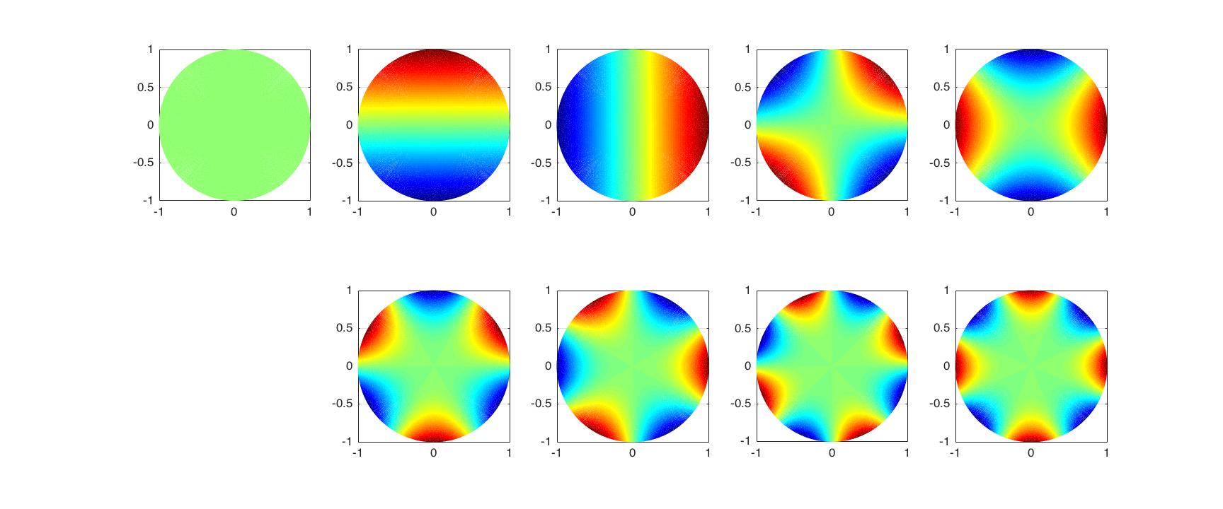
Figure 1: The first nine Steklov eigenfunctions on a unit circle.

3.2 On an Annulus

When $\Omega=B(0,1)\setminus B(0,\epsilon)$, the Steklov eigenvalues can be found via the method of separation of variables [7]. The only eigenfunction which is radial independent satisfies

$$u(r)=(\frac{-(1+\epsilon)}{\epsilon\ln\epsilon})\ln(r)+1,$$

and the corresponding eigenvalue is

$$\lambda=\frac{1+\epsilon}{\epsilon}\ln(1/\varepsilon).$$

The rest of the eigenfunctions are of the form

$$u_{k}(r,\theta)=(Ar^{k}+Br^{-k})H(k\theta),\quad k\in\mathbb{N}$$ (9)

where $A$ and $B$ are constants and $H(k\theta)=\cos(k\theta)$ or $H(k\theta)=\sin(k\theta)$. The boundary conditions become

$$\frac{\partial}{\partial_{r}}u_{k}(1,\theta) = \lambda\,u_{k}(1,\theta),$$

$$\frac{\partial}{\partial_{r}}u_{k}(\epsilon,\theta) = -\lambda\,u_{k}(\epsilon,\theta),$$ (10)

which can be simplified to the following system

$$\left[\begin{array}[]{cc}\lambda\epsilon^{k}+k\epsilon^{k-1}&\lambda\epsilon^{-k}-k\epsilon^{-k-1}\\ \lambda-k&\lambda+k\end{array}\right]\left[\begin{array}[]{c}A\\ B\end{array}\right]=\left[\begin{array}[]{c}0\\ 0\end{array}\right].$$

To obtain nontrivial solutions, the determinant of the matrix needs to be zero. Thus Steklov eigenvalues are determined by the roots of the following polynomial

$$p_{k}(\lambda)=\lambda^{2}-\lambda k\left(\frac{\epsilon+1}{\epsilon}\right)\left(\frac{1+\epsilon^{2k}}{1-\epsilon^{2k}}\right)+\frac{1}{\epsilon}k^{2},\quad k\in\mathbb{N}.$$ (11)

Note that every root corresponds to a double eigenvalue. If $\epsilon>0$ is smaller enough, for $k=1$, we get the smallest eigenvalue

$$\lambda_{1}(\Omega)=\frac{1}{2\epsilon}\frac{1+\epsilon^{2}}{1-\epsilon}\left(1-\sqrt{1-4\epsilon\left(\frac{1-\epsilon}{1+\epsilon^{2}}\right)^{2}}\right).$$

3.3 Shape Optimization

It follows from (2) that the Steklov eigenvalues satisfy the homothety property $\lambda_{k}(t\Omega)=t^{-1}\lambda_{k}(\Omega).$ Instead of fixing the perimeter or the area, one can consider the following shape optimization problems

$$\lambda_{k}^{L\star}=\underset{\Omega\subset\mathbb{R}^{2}}{\text{max}}\lambda_{k}^{L}(\Omega)\qquad\text{where $\lambda_{k}^{L}(\Omega)$=$\lambda_{k}(\Omega)\left|\partial\Omega\right|$}$$ (12)

and

$$\lambda_{k}^{A\star}=\underset{\Omega\subset\mathbb{R}^{2}}{\text{max}}\lambda_{k}^{A}(\Omega)\qquad\text{where $\lambda_{k}^{A}(\Omega)$=$\lambda_{k}(\Omega)\sqrt{\left|\Omega\right|}$}.$$ (13)

As mentioned in the Introduction section, the perimeter eigenvalue problem (12) is known analytically for simply-connected domains. Thus, we focus only on normalized eigenvalue with respect to the area as described in (13).

3.3.1 On an Annulus

In Section 3.2 we get $\lambda_{1}(\Omega)$ on an annulus $\Omega=B(0,1)\setminus B(0,\epsilon)$. Thus, $\lambda_{1}^{L}=\lambda_{1}[2\pi(1+\epsilon)]$ is the normalized first eigenvalue with respect to the perimeter of the domain $\Omega$. The perimeter normalized eigenvalue is not a monotone function in $\epsilon$ and it reaches the maximum value $6.8064$ when $\epsilon=\epsilon^{*}\approx 0.1467$ [7] as shown in Figure 2. On the other hand $\lambda_{1}^{A}=\lambda_{1}[\sqrt{\pi(1-\epsilon^{2})}]$ is the normalized first eigenvalue with respect to the area of the domain $\Omega$ which turns out to be a monotone decreasing function in $\epsilon$ and it reaches the maximum value $\sqrt{\pi}$ when $\epsilon=0$ as shown in Figure 2.

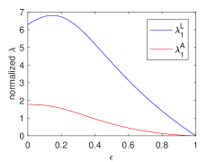
Figure 2: The perimeter- and area-normalized eigenvalue, $\lambda_{1}^{L}$ and $\lambda_{1}^{A}$, on an annulus, respectively.

3.3.2 Shape derivative

Here we review the concept of the shape derivative. For more details, we refer the readers to [22].

Definition: Let $\Omega\subset\mathbb{R}^{N}$ and $J$ be a functional on $\Omega\mapsto J(\Omega)$. Consider the perturbation $x\in\Omega\rightarrow x+tV\in\Omega_{t}$ where $V$ is a vector field. Then the shape derivative of the functional $J$ at $\Omega$ in the direction of a vector field $V$ is given by

$$dJ(\Omega;V)=\underset{t\downarrow 0}{lim}\frac{J(\Omega_{t})-J(\Omega)}{t}.$$ (14)

In [10], the shape derivative of Steklov eigenvalue is given by the following proposition.

Proposition: Consider the perturbation $x\mapsto x+tV$ and denote $c=V\cdot\hat{n}$ where $\hat{n}$ is the outward unit normal vector. Then a simple (unit-normalized) Steklov eigenpair $\left(\lambda,u\right)$ satisfies the perturbation formula

$$\lambda(\Omega)^{\prime}=\int_{\partial\Omega}(\left|\nabla u\right|^{2}-2\lambda^{2}u^{2}-\lambda\kappa u^{2})c\,ds$$ (15)

where $\kappa$ is the mean curvature.

Proof. By using the variational formulation (2) of eigenvalue and normalizing the eigenfunction by

$$\int_{\partial\varOmega}u^{2}ds=1,$$ (16)

we have

$$\lambda(\Omega)=\int_{\Omega}\left|\nabla u\right|dx.$$

Now denote the shape derivative by the prime, thus

$$\begin{array}[]{rclcc}\lambda^{\prime}(\Omega)&=&\left(\int_{\Omega}\left|\nabla u\right|^{2}dx\right)^{\prime}&&(\text{shape derivative)}\\ \\ &=&\int_{\Omega}(\left|\nabla u\right|^{2})^{\prime}dx+\int_{\partial\Omega}\left|\nabla u\right|^{2}V\cdot n\,ds\\ \\ &=&\int_{\Omega}(\nabla u\cdot\nabla u)^{\prime}dx+\int_{\partial\Omega}\left|\nabla u\right|^{2}V\cdot n\,ds\\ \\ &=&2\int_{\Omega}\nabla u\cdot(\nabla u)^{\prime}dx+\int_{\partial\Omega}\left|\nabla u\right|^{2}c\,ds\\ \\ &=&-2\int_{\Omega}(\triangle u)u^{\prime}dx+2\int_{\partial\Omega}u_{n}u^{\prime}ds+\int_{\partial\Omega}\left|\nabla u\right|^{2}c\,ds&&(\text{Green's identity)}\\ \\ &=&2\lambda\int_{\partial\Omega}uu{}^{\prime}ds+\int_{\partial\Omega}\left|\nabla u\right|^{2}c\,ds&&\text{( Equation (\ref{eq:Steklov eigenvalue}) )}\end{array}$$

Now applying the shape derivative to (16), we get

$$\int_{\partial\Omega}uu^{\prime}\,ds=-\int_{\partial\Omega}\left(uu_{n}+\frac{\kappa}{2}\right)u^{2}c\,ds=-\int_{\partial\Omega}\left(\lambda+\frac{\kappa}{2}\right)u^{2}c\,ds$$

Therefore, we get (15) where $\kappa$ is the mean curvature.

Now consider the optimization problem (13) and use the shape derivative of $\lambda$, we get

$$\begin{array}[]{rl}\left(\lambda_{k}^{A}(\Omega)\right)^{\prime}&=\left(\lambda_{k}(\Omega)\cdot\sqrt{\left|\Omega\right|}\right)^{\prime}\\ \\ &=\lambda_{k}^{\prime}(\Omega)\sqrt{\left|\Omega\right|}+\lambda_{k}(\Omega)\frac{1}{2\sqrt{\left|\Omega\right|}}\Omega^{\prime}\\ \\ &=\sqrt{\left|\Omega\right|}\int_{\partial\Omega}\left(\left|\nabla u\right|^{2}-2\lambda^{2}u^{2}-\lambda\kappa u^{2}\right)c\,ds+\lambda_{k}(\Omega)\frac{1}{2\left|\Omega\right|}\int_{\partial\Omega}c\,ds\\ \\ &=\sqrt{\left|\Omega\right|}\int_{\partial\Omega}\left(\left(\left|\nabla u\right|^{2}-2\lambda^{2}u^{2}-\lambda\kappa u^{2}\right)+\lambda_{k}(\Omega)\frac{1}{2\left|\Omega\right|}\right)c\,ds.\end{array}$$ (17)

Thus the normalized velocity for the ascent direction can be chosen as

$$c=V_{n}=\left(\left|\nabla u\right|^{2}-2\lambda^{2}u^{2}-\lambda\kappa u^{2}\right)+\lambda_{k}(\Omega)\frac{1}{2\left|\Omega\right|}.$$ (18)

Later we will show how to use this velocity $V_{n}$ to find the optimal domain which maximizes normalized $k-$th Steklov eigenvalue with respect to the area for a given $k.$

4 Steklov Eigenvalue Problems on the Complex Plane

4.1 On a Simply-Connected Domain

In this section, we formulate the Steklov eigenvalue problem on the complex plane $\mathbb{C}$ instead of $\mathbb{\mathbb{R}}^{2}.$ Consider the Steklov eigenvalue problem (1) on a simply-connected domain $\Omega\subset\mathbb{C}.$ Due to the Riemann Mapping Theorem that guarantees the existence of a unique conformal mapping between any two simply-connected domains, we denote $f=f(\omega)$ as the mapping function that maps the interior of a unit circle $|\omega|=1$ where $w=re^{i\theta}=\xi+i\eta$ to the interior of $\Omega$. Furthermore, every harmonic function is the real part of an analytic function, $u=\Re\{\Psi\}$ where $\Psi$ is the complex potential and $\Re\{\Psi\}$ denotes the real part of the argument $\Psi$. The advantage of this formulation is that we no longer need to solve the equation on $\Omega$ as $u$ satisfies the Laplace’s equation automatically. We only need to find the solution satisfies the boundary condition.

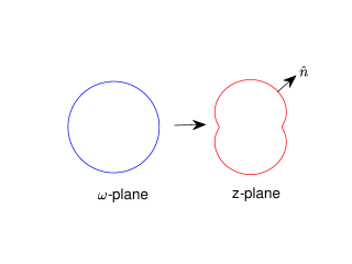
Figure 3: The mapping from a unit circle on $\omega-$plane to a simply-connected domain on $z-$plane.

Parametrizing the boundary of the original domain $\Omega$ with $z(\theta)=x(\theta)+iy(\theta)=f(\omega)$, $\mid\omega\mid=1$ as shown in Figure 3. The outward unit normal is

$$\hat{n}=(\frac{\dot{y}}{\sqrt{\dot{y}^{2}+\dot{x}^{2}}},\frac{-\dot{x}}{\sqrt{\dot{y}^{2}+\dot{x}^{2}}})$$

where $\dot{x}=\frac{dx}{d\theta}$, $\dot{y}=\frac{dy}{d\theta}$ and the gradient of $u$ is

$$\nabla_{z}u=u_{x}+iu_{y}.$$

Thus the derivative in the normal direction is given by

$$\hat{n}\cdot\nabla_{z}u=\Im\left\{(\frac{\dot{x}+i\dot{y}}{\sqrt{\dot{x}^{2}+\dot{y}^{2}}})(u_{x}-iu_{y})\right\}=\Im\left\{\frac{\dot{z}}{\left|f_{\omega}\right|}\overline{\nabla_{z}u}\right\}$$ (19)

where $\Im(\cdot)$ denotes the imaginary part of the argument. Since, $z=f(w)$, we have $\dot{z}=f_{\omega}\dot{\omega}=if_{\omega}\omega$ and $\overline{\nabla_{z}u}=\Psi_{z}=\Psi_{\omega}/f_{\omega}.$ Thus, we get

$$\hat{n}\cdot\nabla_{z}u=\Im\left\{\frac{if_{\omega}\omega}{\left|f_{\omega}\right|}\frac{\Psi_{\omega}}{f_{\omega}}\right\}=\Re\left\{\frac{\omega}{\left|f_{\omega}\right|}\Psi_{\omega}\right\}\quad\text{on$\,\left|\omega\right|=1$}.$$

The boundary condition $\frac{\partial u}{\partial n}=\lambda u$ in (1) thus becomes

$$\Re\left\{\omega\Psi_{\omega}\right\}=\lambda\left|f_{\omega}\right|\Re\left\{\Psi\right\}\qquad\text{on}\left|\omega\right|=1.$$ (20)

Note that $\lambda=0$ is an eigenvalue and its corresponding eigenfunction $u=\Re\{\Psi\}$ is a constant function. In this formulation, it is not necessary to solve the harmonic equation as the real part of an analytic function is always harmonic. However, it is required to know the mapping function $f(\omega)$ and solve the equation (20) on the unit circle. In some cases, it is not easy to find a conformal mapping between an arbitrary simply-connected domain and the unit circle. When this happens, the Schwarz–Christoffel transformation [23] can be used to estimate the mapping.

4.2 Steklov Eigenvalues of an Annulus

In Section 3.2, we find Steklov eigenvalues on an annulus $\Omega=B(0,1)\setminus B(0,\epsilon)$ in $\mathbb{R}^{2}$. Here we reformulate the same problem in $\mathbb{C}$ and show that the same equation is obtained for determining the eigenvalues. The boundary conditions (10) in the complex formula are

$$\Re(\omega\Psi_{\omega}) = \,\,\,\lambda\Re(\Psi),\;\text{on $\left|\omega\right|=1$,}$$

$$\Re(\omega\Psi_{\omega}) = -\lambda\Re(\Psi),\;\text{on}\left|\omega\right|=\epsilon.$$ (21)

where $\omega=re^{i\theta}$. Plugging $\Psi=\underset{k}{\sum}a_{k}\omega^{k}$ into (21) leads to

$$\sum_{k}k(a_{k}-\overline{a_{-k}})e^{ik\theta}=\lambda\sum_{k}(a_{k}+\overline{a_{-k}})e^{ik\theta},$$

$$\sum_{k}k(a_{k}\epsilon^{k-1}-\overline{a_{-k}}\epsilon^{-k-1})e^{ik\theta}=-\lambda\sum_{k}(a_{k}\epsilon^{k}+\overline{a_{-k}}\epsilon^{-k})e^{ik\theta},$$

which implies that

$$\left[\begin{array}[]{cc}\lambda\epsilon^{k}+k\epsilon^{k-1}&\lambda\epsilon^{-k}-k\epsilon^{-k-1}\\ \lambda-k&\lambda+k\end{array}\right]\left[\begin{array}[]{c}a_{k}\\ \overline{a_{-k}}\end{array}\right]=\left[\begin{array}[]{c}0\\ 0\end{array}\right].$$

As shown in Section 3.2, the Steklov eigenvalues are determined by the roots of the polynomial (11).

4.3 Shape Optimization Problem

Here we formulate the velocity (18) in the complex plane $\mathbb{C}.$ By using the fact that $\left|\omega\right|^{2}=\bar{\omega}\omega=1$, we obtain

$$\frac{d}{dt}\left(\bar{\omega}\omega\right)=\bar{\omega}_{t}\omega+\bar{\omega}\omega_{t}=2\Re\{\bar{\omega}_{t}\omega\}=0.$$

Since the mapping function is $z=f(\omega,t)$, we have $\frac{dz}{dt}=f_{t}+f_{\omega}\omega_{t}.$ The normal component of the velocity is given by

$$V_{n} =\hat{n}\cdot V=\Im\left\{\frac{if_{\omega}\omega}{|f_{\omega}|}\overline{\left(f_{\omega}\omega_{t}+f_{t}\right)}\right\}=\Re\left\{\frac{f_{\omega}\omega}{|f_{\omega}|}\overline{\left(f_{\omega}\omega_{t}+f_{t}\right)}\right\}$$

$$=\Re\left\{\frac{\overline{f_{\omega}\omega}}{|f_{\omega}|}\left(f_{\omega}\omega_{t}+f_{t}\right)\right\}=\Re\left\{|f_{\omega}|\overline{\omega}\omega_{t}+\frac{f_{t}\left|f_{\omega}\right|}{\omega f_{\omega}}\right\}$$

$$=\Re\left\{\frac{f_{t}\left|f_{\omega}\right|}{\omega f_{\omega}}\right\}.$$

Therefore, the velocity (18) becomes

$$\Re\left\{\frac{f_{t}\mid f_{w}\mid}{wf_{w}}\right\}=\mid\nabla u\mid^{2}-2\lambda^{2}u^{2}-\lambda\kappa u^{2}+\frac{\lambda}{2|\Omega|}$$

where $u$ is the normalized eigenfunction satisfying

$$\int_{\partial\varOmega}u^{2}ds=\int_{|\omega|=1}\left(\Re\left\{\Psi\right\}\right)^{2}|f_{\omega}|d\omega=1.$$ (22)

Thus

$$\Re\left\{\frac{f_{t}}{wf_{w}}\right\}=R(f,\Psi)$$ (23)

where the right hand side function $R(f,\Psi)$ is

$$R(f,\Psi)=\frac{1}{\left|f_{\omega}\right|}\left(\mid\Psi_{\omega}\mid^{2}\frac{1}{\left|f_{\omega}\right|^{2}}-2\lambda^{2}\Re(\Psi)^{2}-\lambda\kappa\Re(\Psi)^{2}+\frac{\lambda}{2|\Omega|}\right),$$

$|\Omega|$ is the area of the given domain and the curvature is

$$\kappa=\frac{\Re\left\{\overline{\omega f_{\omega}}\left(\omega\left(\omega f_{\omega}\right)_{\omega}\right)\right\}}{\left|\omega f_{\omega}\right|^{3}}.$$ (24)

Now, since $f$ is analytic in $\mid\omega\mid<1$ ,

$$\frac{f_{t}}{\omega f_{\omega}}\text{ is analytic in}\left|\omega\right|<1.$$

By using the Poisson integral formula, the value of an analytic function in the domain $\mid\omega\mid<1$ can be obtained in term of its real part evaluated on the unit circle. The equation (23) implies that

$$\frac{f_{t}}{\omega f_{\omega}} =\frac{1}{2\pi i}\oint_{\mid\omega^{\prime}\mid=1}\frac{1}{\omega^{\prime}}\frac{\omega^{\prime}+\omega}{\omega\prime-\omega}\Re\left\{R\left(f\left(\omega^{\prime}\right),\Psi\left(\omega^{\prime}\right)\right)\right\}d\omega^{\prime}$$

$$=\Re\left\{R\left(f\left(\omega\right),\Psi\left(\omega\right)\right)\right\}+i\text{$\mathcal{H}$}\left\{R\left(f\left(\omega\right),\Psi\left(\omega\right)\right)\right\}$$

where

$$\text{$\mathcal{H}$}[R\left(f\left(e^{i\theta}\right),\Psi\left(e^{i\theta}\right)\right)]=\frac{1}{2\pi}\int_{-\pi}^{\pi}\cot(\frac{\theta^{\prime}-\theta}{2})\Re\left\{R\left(f\left(e^{i\theta^{\prime}}\right),\Psi\left(e^{i\theta^{\prime}}\right)\right)\right\}d\theta^{\prime}$$

is the Hilbert transform. Thus we have

$$f_{t}=\omega f_{\omega}(\Re(R\left(f\left(\omega\right),\Psi\left(\omega\right)\right))+i\text{$\mathcal{H}$}[R\left(f\left(\omega\right),\Psi\left(\omega\right)\right)])$$ (25)

which provides the deformation of the domain via the changes of the conformal mapping.

5 Numerical Approaches for Solving Steklov Eigenvalue Problems

In this section, we discuss the details of numerical discretization. Assume $f$ and $\psi$ are represented as series expansions, i.e.

$$f(w)=\sum_{-\infty}^{\infty}a_{k}\omega^{k}\text{ and }\Psi=\sum_{-\infty}^{\infty}c_{k}\omega^{k},$$

respectively. In Section 5.1, we discuss how to find Steklov eigenvalues and eigenfunctions on a given domain which is represented by $z=f(\omega)$, $|\omega|\leq 1$. This requires to find eigenvalues $\lambda$ and analytic functions $\Psi$ whose real part are eigenfunctions in Equation (20) for a given $f.$ In Section 5.2, we discuss how to discretize Equation (23) on a unit circle to obtain a system of ordinary differential equations (ODEs) of the coefficients $a_{k}(t)$ of $f(\omega,t)$ with a given initial guess of $a_{k}(0)$ of $f(\omega,0)$. The stationary state of this system of ODEs gives the optimal area-normalized Steklov eigenvalue.

5.1 Forward Solvers

Given $f(w)=\sum_{-\infty}^{\infty}a_{k}w^{k}$, we solve (20) numerically on $|\omega|=1$ by parametrizing the unit circle by using the angle $\theta$

$$\omega=e^{i\theta},\>\theta=[0,2\pi).$$

Note that $a_{k}=0$ for $k<0$ as the domain is mapping to the interior of the unit circle, i.e. $|\omega|\leq 1.$ The derivative of $f$ can be obtained as

$$f_{\omega}=\sum_{-\infty}^{\infty}ka_{k}\omega^{k-1}$$

and the magnitude of $|f_{\omega}|=\left(f_{\omega}\overline{f_{\omega}}\right)^{\frac{1}{2}}$ can be obtained in a series expansion again. Assume that the series expansion of $|f_{\omega}|$ is

$$|f_{\omega}|=\sum_{-\infty}^{\infty}d_{l}\omega^{l}.$$

Since $|f_{\omega}|$ is real, we must have $d_{l}=\overline{d_{-l}}$. Denote the expansion of $\Psi$ as

$$\Psi=\sum_{-\infty}^{\infty}c_{k}\omega^{k}$$

where $c_{k}=0$ for $k<0$ too. Plugging these series expansions into (20), we have

$$\sum_{-\infty}^{\infty}k(c_{k}-\overline{c_{-k}})\omega^{k}=\lambda\sum_{m=-\infty}^{\infty}\sum_{l=-\infty}^{\infty}(c_{m}+\overline{c_{-m}})d_{l}\omega^{m+l}.$$

We can then use the identity

$$\sum_{m=-\infty}^{\infty}\sum_{l=-\infty}^{\infty}(c_{m}+\overline{c_{-m}})d_{l}\omega^{m+l}=\sum_{k=-\infty}^{\infty}\sum_{m=-\infty}^{\infty}(c_{m}+\overline{c_{-m}})d_{k-m}\omega^{k}.$$

By matching the coefficients of $\omega^{k}$, we have

$$\lambda\sum_{m=-\infty}^{\infty}(c_{m}+\overline{c_{-m}})d_{k-m}=k(c_{k}-\overline{c_{-k}}).$$ (26)

Denote the real and complex part of $c_{n}$, $d_{n}$ by $c_{n}^{r}$, $d_{n}^{r}$ and $c_{n}^{i}$, $d_{n}^{i}$, respectively, we then have

$$\lambda\sum_{m=-\infty}^{\infty}(c_{m}^{r}+ic_{m}^{i}+c_{-m}^{r}-ic_{-m}^{i})(d_{k-m}^{r}+id_{k-m}^{i})=k(c_{k}^{r}+ic_{k}^{i}-c_{-k}^{r}+ic_{-k}^{i}).$$

By comparing real and imaginary parts, we have

$$\left\{\begin{array}[]{ccc}\lambda\sum_{m=-\infty}^{\infty}c_{m}^{r}(d_{k-m}^{r}+d_{k+m}^{r})+c_{m}^{i}(d_{k+m}^{i}-d_{k-m}^{i})&=&kc_{k}^{r},\\ \lambda\sum_{m=-\infty}^{\infty}c_{m}^{r}(d_{k-m}^{i}+d_{k+m}^{i})+c_{m}^{i}(d_{k-m}^{r}-d_{k+m}^{r})&=&kc_{k}^{i}.\end{array}\right.$$ (27)

In numerical computation, the series expansion is carried out numerically by truncating the series expansion at $k=\frac{N}{2}$ and Fast Fourier Transform (FFT) is used to efficiently compute quantities in $\omega-$plane and $z-$plane. Denote $\frac{N}{2}$ as $N_{2}$. Thus

$$f(\omega)\approx\sum_{k=-N_{2}}^{N_{2}}a_{k}\omega^{k}=\sum_{k=-N_{2}}^{N_{2}}a_{k}e^{ik\theta}$$

and

$$f_{\omega}=\sum_{k=-N_{2}}^{N_{2}}ka_{k}\omega^{k-1}.$$

Denote

$$|f_{\omega}|=\sum_{l=-N}^{N}d_{l}\omega^{l}$$

where $d_{l}$, $-N\leq l\leq N$, are obtained by using the pseudo-spectral method. We use inverse Fourier transform (IFFT) to obtain $f_{\omega}$ in physical space and compute $|f_{\omega}|$ in physical space, then use FFT to get $d_{l}$ in Fourier space. The aliasing of a nonlinear product is avoided by adopting the zero-padding.

The system of infinite equations (27) is approximated by the system of finite equations for 0:$N_{2}$-modes which gives

$$\lambda AC=BC$$ (28)

where

$$A_{k+1,m+1} =d_{k-m}^{r}+d_{k+m}^{r},\quad\text{for}\quad 0\leq k\leq N_{2},0\leq m\leq N_{2},$$

$$A_{k+1,m+N_{2}+1} =-d_{k-m}^{i}+d_{k+m}^{i},\quad\text{for}\quad 0\leq k\leq N_{2},1\leq m\leq N_{2},$$

$$A_{k+N_{2}+1,m+1} =d_{k-m}^{i}+d_{k+m}^{i},\quad\text{for}\quad 1\leq k\leq N_{2},0\leq m\leq N_{2},$$

$$A_{k+N_{2}+1,m+N_{2}+1} =d_{k-m}^{r}-d_{k+m}^{r},\quad\text{for}\quad 1\leq k\leq N_{2},1\leq m\leq N_{2},$$

and

$$B_{k+1,m+1} =k\delta_{k,m},\quad\text{for}\quad 0\leq k\leq N_{2},0\leq m\leq N_{2},$$

$$B_{k+1,m+N_{2}+1} =0,\quad\text{for}\quad 0\leq k\leq N_{2},1\leq m\leq N_{2},$$

$$B_{k+N_{2}+1,m+1} =0,\quad\text{for}\quad 1\leq k\leq N_{2},0\leq m\leq N_{2},$$

$$B_{k+N_{2}+1,m+N_{2}+1} =k\delta_{k,m},\quad\text{for}\quad 1\leq k\leq N_{2},1\leq m\leq N_{2},$$

and

$$C=\left[\begin{array}[]{c}C^{r}\\ C^{i}\end{array}\right]$$

where

$$C^{r}=\left[\begin{array}[]{c}c_{0}^{r}\\ c_{1}^{r}\\ c_{2}^{r}\\ \vdots\\ c_{N_{2}}^{r}\end{array}\right],\quad C^{i}=\left[\begin{array}[]{c}c_{0}^{i}\\ c_{1}^{i}\\ c_{2}^{i}\\ \vdots\\ c_{N_{2}}^{i}\end{array}\right].$$

By solving the linear system (28) we could find the coefficient vector $C$ and its corresponding eigenvalue $\lambda$. We assign zero values for $c_{k}^{r}$ and $c_{k}^{i}$ for $k>N_{2}.$ Thus the corresponding eigenfunction will be given by $u=\Re\{\Psi\}=\Re\{\sum_{-N_{2}}^{N_{2}}c_{k}\omega^{k}\}.$

Now, if we assume that the coefficients $d_{n}$ are real we will be able to reduce the matrix size and solve the problem even more efficiently. In this case, we have

$$\left\{\begin{array}[]{ccc}\lambda\sum_{m=0}^{N_{2}}c_{m}^{r}(d_{k-m}+d_{k+m})&=&kc_{k}^{r},\\ \lambda\sum_{m=1}^{N_{2}}c_{m}^{i}(d_{k-m}-d_{k+m})&=&kc_{k}^{i}.\end{array}\right.$$ (29)

The 0:$N_{2}$-modes approximation gives

$$\lambda A^{r}C^{r}=B^{r}C^{r},\lambda A^{i}C^{i}=B^{i}C^{i},$$

where

$$A_{k+1,m+1}^{r}=d_{k-m}+d_{k+m},\quad B_{k+1,m+1}^{r}=k\delta_{k,m}\quad\text{for}\quad 0\leq k\leq N_{2},0\leq m\leq N_{2},$$

$$A_{k,m}^{i}=d_{k-m}-d_{k+m},\quad B_{k,m}^{i}=k\delta_{k,m},\quad\text{for}\quad 0\leq k\leq N_{2},0\leq m\leq N_{2},$$

and

$$C^{r}=\left[\begin{array}[]{c}c_{0}^{r}\\ c_{1}^{r}\\ c_{2}^{r}\\ \vdots\\ c_{N_{2}}^{r}\end{array}\right],\quad C^{i}=\left[\begin{array}[]{c}c_{0}^{i}\\ c_{1}^{i}\\ c_{2}^{i}\\ \vdots\\ c_{N_{2}}^{i}\end{array}\right].$$

5.2 Optimization Solvers

In this section, we discuss how to solve the dynamic equation (25) by method of lines and spectral method in the variable $\omega$. Given a conformal mapping $f(\omega,t)=\sum_{-N_{2}}^{N_{2}}a_{k}(t)\omega^{k}$, we use the method discussed in 5.1 to obtain $k$th eigenvalue $\lambda_{k}$, its corresponding eigenfunction $u_{k}=\Re\{\Psi\}$ where $\Psi(w,t)=\sum_{-N_{2}}^{N_{2}}c_{k}(t)\omega^{k}$. Notice that this eigenfunction is not normalized. To find the normalization constant, we compute the Fourier coefficient representation of

$$\left(\Re\left\{\Psi\right\}\right)^{2}|f_{\omega}|=\sum_{-N_{2}}^{N_{2}}b_{k}(t)\omega^{k}$$

via a pseudo-spectral method and then the normalization condition (22) is approximated by

$$\int_{|\omega|=1}\left(\Re\left\{\Psi\right\}\right)^{2}|f_{\omega}|d\omega\approx 2\pi b_{0}(t).$$

The normalized eigenfunction $u=\Re\left\{\tilde{\Psi}\right\}$ where

$$\tilde{\Psi}(w,t)=\sum_{-N_{2}}^{N_{2}}\frac{1}{\sqrt{2\pi b_{0}}}c_{k}(t)\omega^{k}=\sum_{-N_{2}}^{N_{2}}\tilde{c}_{k}(t)\omega^{k}.$$

The curvature term can be computed via the formula (24) by using the following expansions

$$\omega f_{\omega}=\sum_{-N_{2}}^{N_{2}}ka_{k}(t)\omega^{k}$$

$$\omega\left(\omega f_{\omega}\right)_{\omega}=\sum_{-N_{2}}^{N_{2}}k^{2}a_{k}(t)\omega^{k}.$$

The area term is obtained by

$$|\Omega|=\sum_{-N_{2}}^{N_{2}}\pi k|a_{k}|^{2}.$$

Plugging

$$|f_{\omega}|=\sum_{-N}^{N}d_{l}\omega^{l},\quad\tilde{\Psi}_{\omega}=\sum_{-N_{2}}^{N_{2}}k\tilde{c}_{k}(t)\omega^{k},$$

the eigenvalue, the curvature, and the area into the right hand side of (23), we obtain $R(f,\tilde{\Psi})$ in terms of Fourier series. All the nonlinear term is obtained by using pseudo-spectral method. We then use discrete Hilbert transform to find the complex conjugate of $R(f,\tilde{\Psi})$ and then compute the right hand side of (25). Denote the series expansion of the right hand side as

$$wf_{w}(\Re\left\{R\left(f(\omega),\tilde{\Psi}(\omega\right)\right\})+i\text{$\mathcal{H}$}[R\left(f(\omega),\tilde{\Psi}(\omega\right)])=\sum_{-N_{2}}^{N_{2}}r_{k}(t)\omega^{k}.$$

Note that $r_{k}$ depends on time and $a_{k}$, $-N_{2}\leq k\leq N_{2}$. Since $f_{t}(\omega,t)=\sum_{-\infty}^{\infty}a_{k}^{\prime}(t)\omega^{k}$, the dynamic equation (25) becomes a system of $N+1$ nonlinear ODEs in Fourier Coefficients

$$a_{k}^{\prime}(t)=r_{k}(t),-N_{2}\leq k\leq N_{2}.$$ (30)

6 Numerical Results

6.1 Forward Solvers

Here we first test our forward solvers on various domains to demonstrate the spectral convergence of the numerical approaches described in Section 5.1. We verify the accuracy of the code by testing the first $12$ eigenvalues on smooth shapes.

6.1.1 Steklov Eigenvalues on a Unit Disk

When we consider the unit circle, the mapping function is $f(\omega)=\omega$ which gives $|f_{\omega}|=1.$ Thus $d_{0}=1$ and $d_{l}=0$ for all $l\neq 0.$ The system of equations (29) becomes

$$\left\{\begin{array}[]{ccc}\lambda c_{k}^{r}=kc_{k}^{r},&&k=0,1,2,3,...\\ \lambda c_{k}^{i}=kc_{k}^{i},&&k=1,2,3,....\end{array}\right.$$ (31)

If $\lambda=0$, $c_{k}^{r}=c_{k}^{i}=0$ for all positive integer and $c_{0}^{r}$ is an arbitrary constant. If $\lambda$ is a particular integer $k_{1}$, i.e., $\lambda=k_{1},$ we must have

$$c_{k}^{r}=c_{k}^{i}=0\quad\text{for}\quad k\neq k_{1},$$

and $c_{k_{1}}^{r}$ and $c_{k_{1}}^{i}$ are arbitrary constants. Thus, Steklov eigenvalue for the unit circle are

$$0,1,1,2,2,3,3,\cdots,k_{1},k_{1},\cdots.$$

The normalized eigenvalues $\lambda_{k}^{A}(\Omega)=\lambda\sqrt{\mid\Omega\mid}$ are listed in Table 1. It is clear that spectral accuracy is observed from the numerical results and the errors only contain round off errors $O(10^{-16})$ on double-precision arithmetic.

$N$	24	25	212	Exact
$\lambda_{0}$	0	0	0	$0$
$\lambda_{1}$	1.772453850905515	1.772453850905515	1.772453850905515	1.772453850905516
$\lambda_{2}$	1.772453850905515	1.772453850905515	1.772453850905515	1.772453850905516
$\lambda_{3}$	3.544907701811031	3.544907701811031	3.544907701811031	3.544907701811032
$\lambda_{4}$	3.544907701811031	3.544907701811031	3.544907701811031	3.544907701811032
$\lambda_{5}$	5.317361552716547	5.317361552716547	5.317361552716547	5.317361552716548
$\lambda_{6}$	5.317361552716547	5.317361552716547	5.317361552716547	5.317361552716548
$\lambda_{7}$	7.089815403622062	7.089815403622062	7.089815403622062	7.089815403622064
$\lambda_{8}$	7.089815403622062	7.089815403622062	7.089815403622062	7.089815403622064
$\lambda_{\text{9}}$	8.862269254527577	8.862269254527577	8.862269254527577	8.862269254527579
$\lambda_{10}$	8.862269254527577	8.862269254527577	8.862269254527577	8.862269254527579
$\lambda_{11}$	10.634723105433094	10.634723105433094	10.634723105433094	10.634723105433096

Table 1: The first 12 eigenvalues $\lambda_{k},k=0,\ldots,11$ for different numbers of grid points $N=2^{n},n=4,5,12$ on a unit circle.

6.1.2 Steklov Eigenvalues on a Shape with 2-Fold Rotational Symmetry

We use the mapping $f(w)=w+0.05w^{3}$ to generate a shape with 2-fold rotational symmetry as shown in Figure 4(a). In Table 2 we summarize the numerical results of Steklov eigenvalues. We use the eigenvalues computed by using $2^{12}$ grids as true eigenvalues and show the log-log plot of errors of the first 12 eigenvalues, i.e.

$$\text{error=}|\lambda_{k}^{N}-\lambda_{k}^{2^{12}}|,k=0,\ldots,11,$$

versus number of grid points $N=2^{4},2^{5},...2^{11}$ in Figure 4(b). It is clear that the spectral accuracy is achieved.

(a)

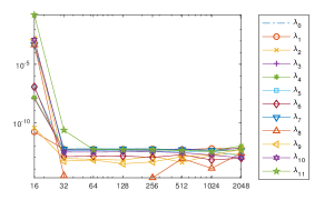
(b)

Figure 4: (a) The 2-fold rotational symmetry shape with $f(w)=w+0.05w^{3}$,$|\omega|\leq 1.$ (b) The log-log plot of errors for the first 11 non-zero eigenvalues versus number of grid points $N=2^{n},n=4,\ldots,11.$

$N$	24	25	26	27
$\lambda_{0}$	0	0	0	$0$
$\lambda_{1}$	1.643146123296456	1.643146123280263	1.643146123280263	1.643146123280268
$\lambda_{2}$	1.904409864808107	1.904409864772927	1.904409864772939	1.904409864772950
$\lambda_{3}$	3.509482564053473	3.509482552385534	3.509482552385528	3.509482552385548
$\lambda_{4}$	3.567218990382545	3.567218976359059	3.567218976359065	3.567218976359050
$\lambda_{5}$	5.298764914769874	5.298764805372437	5.298764805372433	5.298764805372439
$\lambda_{6}$	5.316931803045312	5.316931688027542	5.316931688027550	5.316931688027557
$\lambda_{7}$	7.074710761837761	7.074238491011210	7.074238491011200	7.074238491011197
$\lambda_{8}$	7.079268312074488	7.078792636301956	7.078792636301953	7.078792636301953
$\lambda_{\text{9}}$	8.846269410836159	8.844970458352126	8.844970458352138	8.844970458352106
$\lambda_{10}$	8.847598359495487	8.846297249970153	8.846297249970146	8.846297249970162
$\lambda_{11}$	10.793832137331764	10.614565359904542	10.614565359883139	10.614565359883118

$N$	28	29	210	212
$\lambda_{0}$	0	0	0	0
$\lambda_{1}$	1.643146123296456	1.643146123280306	1.643146123280187	1.643146123280772
$\lambda_{2}$	1.904409864772878	1.904409864772972	1.904409864773167	1.904409864773008
$\lambda_{3}$	3.509482552385497	3.509482552385653	3.509482552385503	3.509482552385095
$\lambda_{4}$	3.567218976359074	3.567218976358907	3.567218976358941	3.567218976358544
$\lambda_{5}$	5.298764805372470	5.298764805372484	5.298764805372494	5.298764805372812
$\lambda_{6}$	5.316931688027525	5.316931688027596	5.316931688027485	5.316931688027425
$\lambda_{7}$	7.074238491011203	7.074238491011272	7.074238491011313	7.074238491011736
$\lambda_{8}$	7.078792636301955	7.078792636302032	7.078792636301965	7.078792636301953
$\lambda_{\text{9}}$	8.844970458352119	8.844970458352195	8.844970458352252	8.844970458352078
$\lambda_{10}$	8.846297249970174	8.846297249970114	8.846297249970023	8.846297249969862
$\lambda_{11}$	10.614565359883121	10.614565359883064	10.614565359882992	10.614565359882672

Table 2: The first 12 eigenvalues $\lambda_{k},k=0,\ldots,11$ for different numbers of grid points $N=2^{n},n=4,\ldots,10,12$ on $f(w)=w+0.05w^{3}$, $|\omega|\leq 1.$

6.1.3 Steklov Eigenvalues on a Shape with 5-Fold Rotational Symmetry

We use the mapping $f(w)=8+5w+0.5w^{6}$ to generate a shape with 5-fold rotational symmetry as shown in Figure 5(a). In Table 3, we use the eigenvalues computed by using $2^{12}$ grids as true eigenvalues and show the log-log plot of errors of the first 12 eigenvalues, i.e.

$$\text{error=}|\lambda_{k}^{N}-\lambda_{k}^{2^{12}}|,k=0,\ldots,11,$$

versus number of grid points $N=2^{4},2^{5},...2^{11}$ in Figure 5(b). It is clear that the spectral accuracy is achieved.

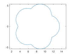
(a)

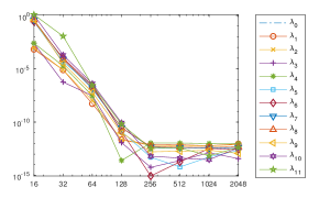
(b)

Figure 5: (a) The 5-fold rotational symmetry shape with $f(w)=8+5w+0.5w^{6}$,$|\omega|\leq 1.$ (b) The log-log plot of errors for the first 11 non-zero eigenvalues versus number of grid points $N=2^{n},n=4,\ldots,11.$

$N$	24	25	26	27
$\lambda_{0}$	0	0	0	$0$
$\lambda_{1}$	1.613981749710263	1.614659735134658	1.614651857980075	1.614651852652450
$\lambda_{2}$	1.615586942999712	1.614659740601958	1.614651863407194	1.614651852652469
$\lambda_{3}$	2.979901447266664	2.977376794062662	2.977377396867629	2.977377367030917
$\lambda_{4}$	2.979920850098075	2.977396410343160	2.977377396867634	2.977377367030926
$\lambda_{5}$	5.757902735512396	5.483423114699104	5.483379266795433	5.483378986137383
$\lambda_{6}$	5.757963817902539	5.483478476088597	5.483379266795448	5.483378986137454
$\lambda_{7}$	7.091240897150815	6.707817046860952	6.707738934321966	6.707738797445765
$\lambda_{8}$	7.092066936388594	6.707817092425547	6.707738981978962	6.707738797445767
$\lambda_{\text{9}}$	8.053537400023426	7.657772022224528	7.657739872866688	7.657739809188358
$\lambda_{10}$	10.114031561463605	9.019776832943990	9.019583333936978	9.019582922824695
$\lambda_{11}$	11.339690354808871	10.150431507211664	10.138974110712084	10.138973824292398

$N$	28	29	210	212
$\lambda_{0}$	0	0	0	0
$\lambda_{1}$	1.614651852650946	1.614651852650901	1.614651852650762	1.614651852650156
$\lambda_{2}$	1.614651852650962	1.614651852650941	1.614651852650909	1.614651852650308
$\lambda_{3}$	2.977377367029736	2.977377367029755	2.977377367029867	2.977377367029730
$\lambda_{4}$	2.977377367029792	2.977377367029804	2.977377367029905	2.977377367030901
$\lambda_{5}$	5.483378986124044	5.483378986123986	5.483378986124047	5.483378986123992
$\lambda_{6}$	5.483378986124095	5.483378986124115	5.483378986124439	5.483378986124096
$\lambda_{7}$	6.707738797416523	6.707738797416477	6.707738797416426	6.707738797416075
$\lambda_{8}$	6.707738797416656	6.707738797416588	6.707738797416567	6.707738797416147
$\lambda_{\text{9}}$	7.657739809178596	7.657739809178618	7.657739809178663	7.657739809178431
$\lambda_{10}$	9.019582922738280	9.019582922738174	9.019582922738246	9.019582922738216
$\lambda_{11}$	10.138973824227390	10.138973824227429	10.138973824227113	10.138973824227044

Table 3: The first 12 eigenvalues $\lambda_{k},k=0,\ldots,11$ for different numbers of grid points $N=2^{n},n=4,\ldots,10,12.$

6.1.4 Steklov Eigenvalues on a Cassini Oval.

All of aforementioned examples have finite terms expansion in $\omega$. Here we show an example with infinite terms expansion in $\omega.$ The mapping $f(w)=\alpha w(\frac{2}{1+\alpha^{2}-(1-\alpha^{2})w^{2}})^{\frac{1}{2}}$ , where $\alpha=0.4$ is used to generate a Cassini Oval shape which is shown in Figure 6(a). In Table 4 we use the eigenvalues computed by using $2^{12}$ grids as true eigenvalues and show the log-log plot of errors of the first 12 eigenvalues, i.e.

$$\text{error=}|\lambda_{k}^{N}-\lambda_{k}^{2^{12}}|,k=0,\ldots,11,$$

versus number of grid points $N=2^{4},2^{5},...2^{10}$ in Figure 6(b). It is also clear that the spectral accuracy is achieved.

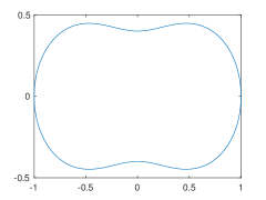
(a)

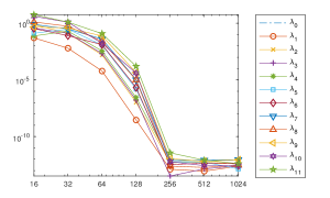
(b)

Figure 6: (a) Cassini oval shape with $f(w)=\alpha w(\frac{2}{1+\alpha^{2}-(1-\alpha^{2})w^{2}})^{\frac{1}{2}}$ ,$|\omega|\leq 1$, and $\alpha=0.4$. (b) The log-log plot of errors for the first 11 non-zero eigenvalues versus number of grid points $N=2^{n},n=4,\ldots,10.$

$N$	24	25	26	27
$\lambda_{0}$	0	0	0	$0$
$\lambda_{1}$	0.872759997500228	0.827902995301854	0.821644770560566	0.821583902061334
$\lambda_{2}$	2.124401456784662	2.756054635303737	2.886951802792420	2.888537681079042
$\lambda_{3}$	2.571449696110635	3.077030643209814	2.946970106404462	2.944846781799040
$\lambda_{4}$	3.265821414464841	3.136596486946471	3.338218243465505	3.341726009279193
$\lambda_{5}$	4.418763601488365	4.854880686612021	4.562691155962767	4.550749526079698
$\lambda_{6}$	5.378320687602239	4.955570564610835	5.023787664833372	5.036737477441735
$\lambda_{7}$	7.025574559110670	6.548839953593787	6.273463980936640	6.233063933209499
$\lambda_{8}$	7.626882523375537	6.870625350063478	6.299773422917886	6.325481073833819
$\lambda_{\text{9}}$	8.263730860061949	8.196071839036918	7.881197306312033	7.805852388999546
$\lambda_{10}$	12.070450297339713	9.144520167848396	7.891680915128140	7.908376668589532
$\lambda_{11}$	15.149068049247919	10.668830636509751	9.526157620343742	9.404387869498899

$N$	28	29	210	212
$\lambda_{0}$	0	0	0	0
$\lambda_{1}$	0.821583899177118	0.821583899177077	0.821583899177230	0.821583899176988
$\lambda_{2}$	2.888537785769291	2.888537785769243	2.888537785769405	2.888537785769792
$\lambda_{3}$	2.944846615497959	2.944846615497851	2.944846615498256	2.977377367029730
$\lambda_{4}$	3.341726289664183	3.341726289664230	3.341726289664046	3.341726289664970
$\lambda_{5}$	4.550747949109708	4.550747949109686	4.550747949110111	4.550747949110250
$\lambda_{6}$	5.036739639826136	5.036739639826031	5.036739639826076	5.036739639826476
$\lambda_{7}$	6.233053526961343	6.233053526961285	6.233053526961188	6.233053526962100
$\lambda_{8}$	6.325490988924451	6.325490988924394	6.325490988924508	6.325490988924206
$\lambda_{\text{9}}$	7.805807719443767	7.805807719443299	7.805807719443544	7.805807719442640
$\lambda_{10}$	7.908416105951900	7.908416105952249	7.908416105952258	7.908416105952520
$\lambda_{11}$	9.404227647278619	9.404227647275778	9.404227647275357	9.404227647274947

Table 4: The first 12 eigenvalues $\lambda_{k},k=0,\ldots,11$ for different numbers of grid points $N=2^{n},n=4,\ldots,10,12.$

6.2 Optimization Solvers

We solve the nonlinear system of ODEs (30) in Section 5.2 by using the forward Euler method with the time step $h$ to obtain the solution at $t+h.$ We can then repeat this procedure iteratively until it finds the optimal shape. To prevent the spurious growth of the high-frequency modes generated by round-off error, we use 25th-order Fourier filtering and also filter out the coefficients which is below $10^{-14}$ as used in [24] after each iteration.

In Figure 7(a), we show the evolution of optimization of $\lambda_{2}^{A}$ with number of grid points $N=256$. We start with a shape with a two-fold symmetry $f(w)=w+0.5w^{3}$ whose $\lambda_{2}^{A}=1.7791$. The algorithm was able to deform the shape and increase the eigenvalue $\lambda_{2}^{A}$ up to 2.1503. After that, the shape starts to generate kinks. Due to so-called crowding phenomenon [25], the accuracy of the conformal mapping will be effected and the shape will lose its smoothness. Thus, we avoid this problem by smoothing the curvature term $\kappa$ in the $z-$plane based on the moving average method with span $5$. Using this smoothing technique at each iteration helps us to achieve better results as shown in Figure 7(b). In addition to smoothing, we also refine our time steps. We start with an initial time step $h=0.1$ and halve the time step for every time period $T=100$ and compute up to $5T.$ The optimal eigenvalues $\lambda_{k}^{A},k=1,\cdots,7$ are summarized in Table 5 and the optimal shapes which have $k$-fold symmetry are shown in Figure 8. As observed in [10], the domain maximizing the $k-$th Steklov eigenvalue has $k$-fold symmetry, and has at least one axis of symmetry. The $k-$th Steklov eigenvalue has multiplicity 2 if $k$ is even and multiplicity 3 if $k$ $\geq$ 3 is odd. The first few nonzero coefficients of the mapping function $f(w)$ of the optimal shapes are summarized in Table 6 for $\lambda_{2}^{A}-\lambda_{7}^{A}$. When optimizing $\lambda_{k}^{A}$, the optimal coefficients have nonzero values for $a_{1+nk}$ where $n\in\mathbb{N}$.

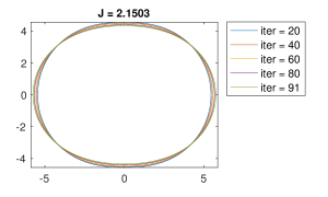
(a)

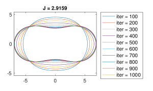
(b)

Figure 7: Optimization of $\lambda_{2}^{A}(\Omega)$ without and with smoothing $k$ are shown on (a) and (b), respectively.

7 Summary and Discussion

We have developed a spectral method based on conformal mappings to a unit circle to solve Steklov eigenvalue problem on general simply-connected domains efficiently. Unlike techniques based on finite difference methods or finite elements methods which requires discretization on the general domains with boundary treatments, the method that we proposed only requires discretization of the boundary of a unit circle. We use a series expansion to represent eigenfunctions so that the discretization leads to an eigenvalue problem for Fourier coefficients. In addition, we study the maximization of area-normalized Steklov eigenvalue $\lambda_{k}^{A}$ based on shape derivatives and formulate this shape evolution in the complex plane via the gradient ascent approach. With smoothing technique and choices of time steps, we were able to find the optimal area-normalized eigenvalues $\lambda_{k}^{A}$ for a given $k$.

As aforementioned, the optimization of Steklov eigenvalue problems on general non-simply-connected domains is a challenge open question. This will require robust and efficient forward solvers of Steklov eigenvalues and numerical techniques to perform shape optimizations which may involve topological changes. In the near future, we plan to explore the possibility in this direction by using Level Set approaches.

$\lambda_{2}^{A}$	$\lambda_{3}^{A}$	$\lambda_{4}^{A}$
0	0	0
0.776986933500041	1.079861668314576	1.171320134341248
2.916071256633050	1.079861668314618	1.171320134341342
2.916071256753514	4.145300664720734	1.611279604736676
3.277492771330297	4.145300664720919	5.284432268416950
4.498623058633566	4.145300672478222	5.284433071016992
5.041166283776032	4.914601402877488	5.448244774262810
6.118061463397883	6.024394262148678	5.448244774262829
6.272697585592614	6.024394262148718	6.489865254319582
7.693637484890079	7.628170417847103	7.335382999100261
7.809873534891437	7.628170417847109	7.335382999100267
9.262237946100434	8.953916828143468	8.636733197287754

$\lambda_{5}^{A}$	$\lambda_{6}^{A}$	$\lambda_{7}^{A}$
0	0	0
1.239226322386241	1.265308570439713	1.291290525113730
1.239226322386290	1.265308570450229	1.291290525113829
1.945145428557867	2.117586845334797	2.250312782549877
1.945145428557917	2.117586845350534	2.250312782549968
6.496444238784153	2.427189796272854	2.777589136940805
6.496444238784278	7.644759577423688	2.777589137507856
6.496444784959914	7.644765127633966	8.846228548846659
6.732142619373287	7.771465908528654	8.846229141938371
6.732142619373318	7.771465908584982	8.846229145378315
8.128106267565293	7.979288943927369	9.050146643762274
8.803176067403113	7.979288943929372	9.050146643762337

Table 5: The optimization of $\lambda_{n}^{A},n=2,\ldots,7$ for the first 12 eigenvalues.

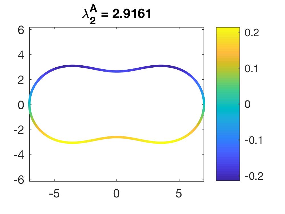
(a)

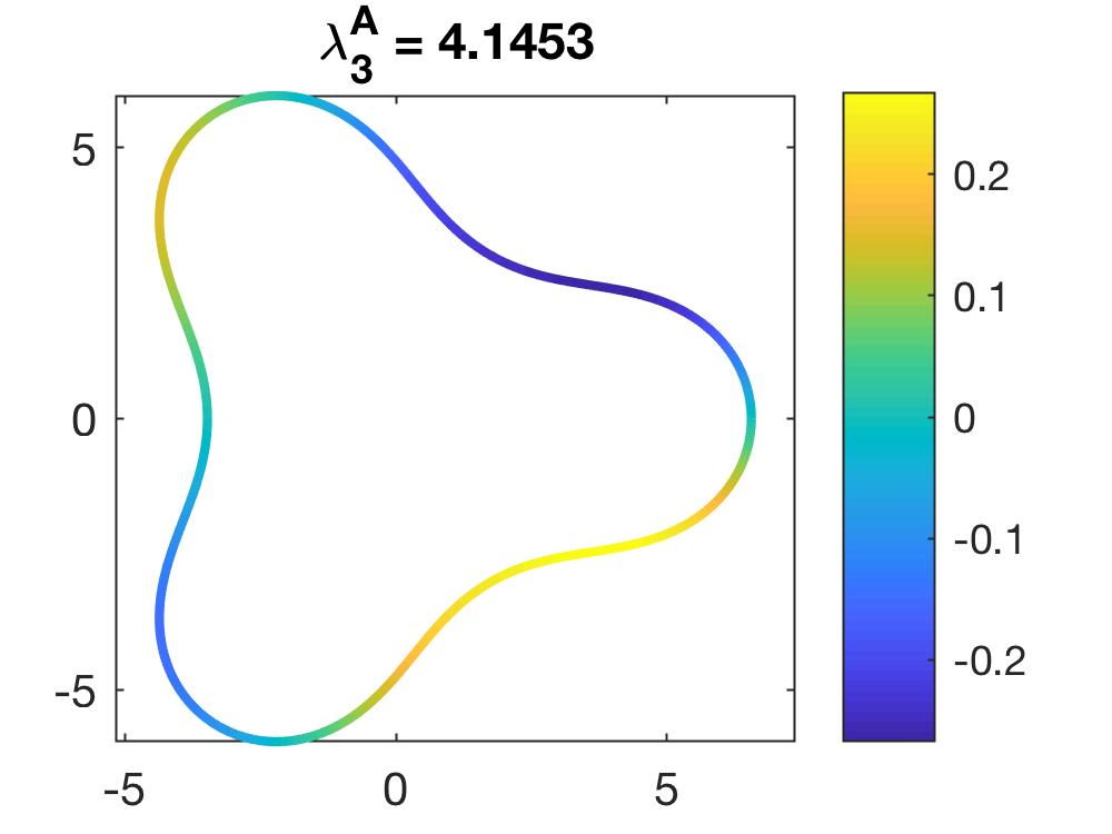
(b)

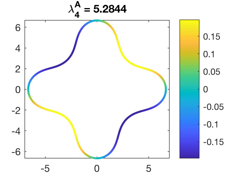
(c)

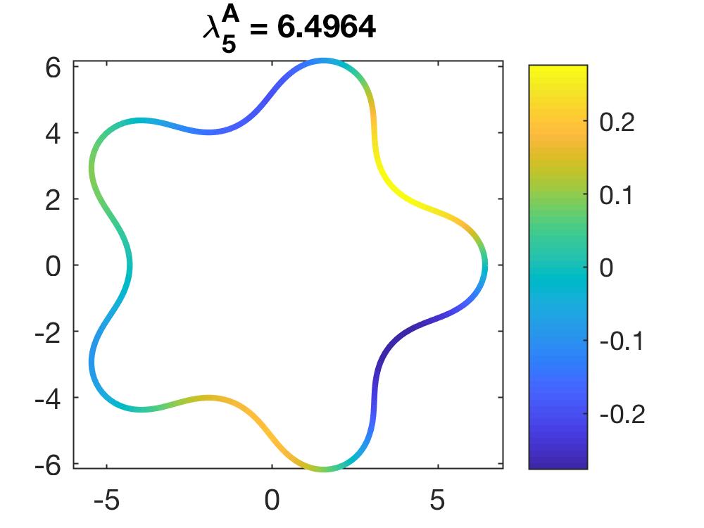
(d)

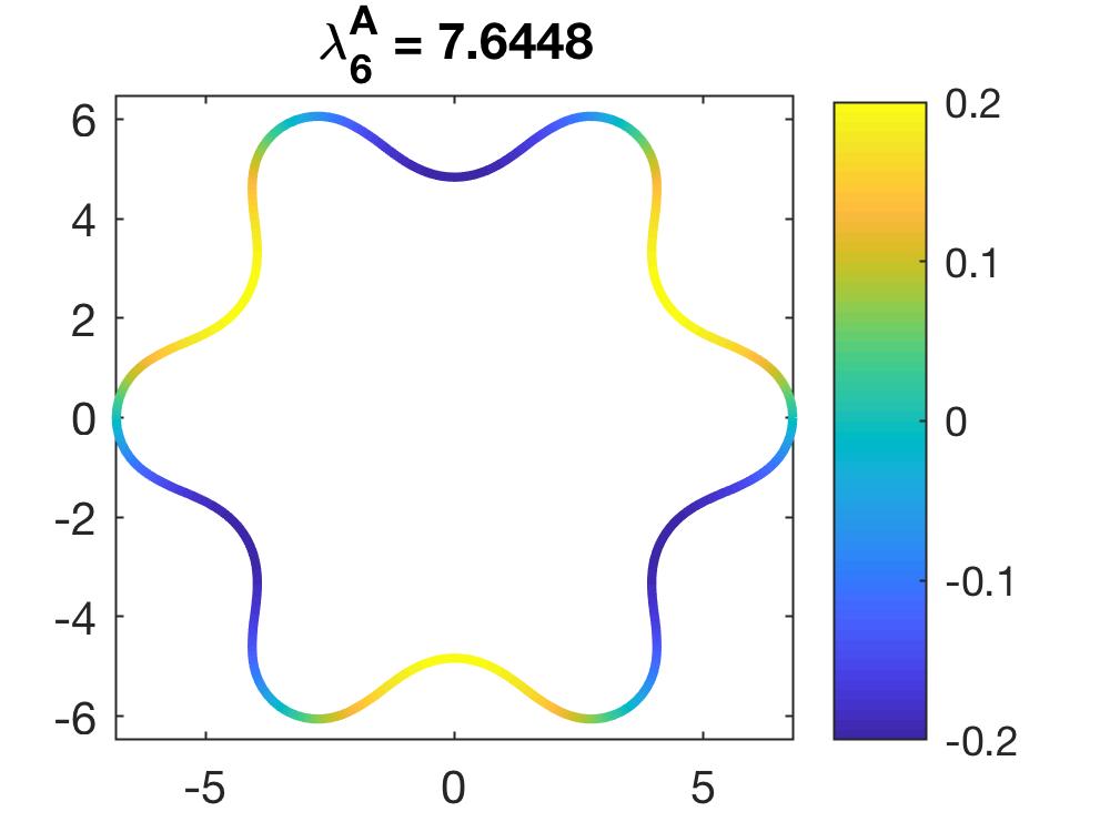
(e)

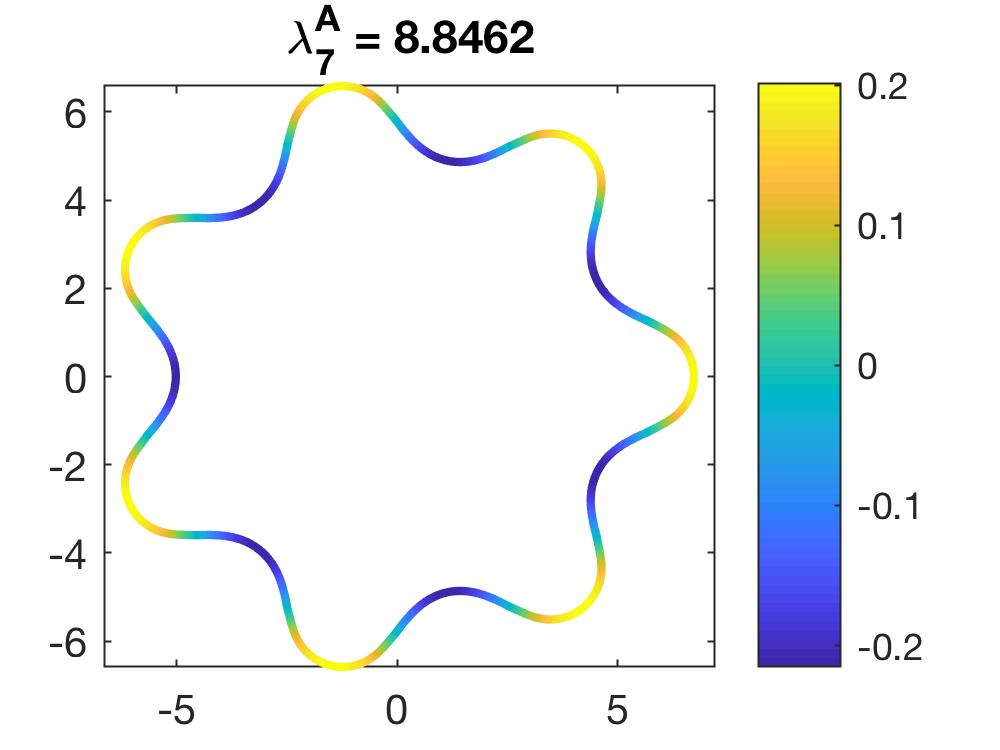
(f)

Figure 8: The optimal shape of maximizing $\lambda_{n}^{A},n=2,\ldots,7.$ The colors on the curve indicate the values of eigenfunctions.

$\lambda_{2}^{A}$		$\lambda_{3}^{A}$		$\lambda_{4}^{A}$
$a_{1}$	3.482625488377397	$a_{1}$	4.172312832330094	$a_{1}$	4.646184610628929
$a_{3}$	1.316760069380197	$a_{4}$	1.018987204748702	$a_{5}$	0.871201920168631
$a_{5}$	0.754288548863893	$a_{7}$	0.514733681728398	$a_{9}$	0.426363809028874
$a_{7}$	0.476336868618610	$a_{12}$	0.301544250312563	$a_{13}$	0.248913034789274
$a_{9}$	0.313178226238119	$a_{15}$	0.187629804532372	$a_{17}$	0.156013896896941
$a_{11}$	0.210225589908090	$a_{18}$	0.120456778256507	$a_{21}$	0.101460942653213
$a_{13}$	0.142829963279173	$a_{21}$	0.078773331531670	$a_{25}$	0.067443016703592
$a_{15}$	0.097776540001909	$a_{24}$	0.052126631797892	$a_{29}$	0.045465744838959

$\lambda_{5}^{A}$		$\lambda_{6}^{A}$		$\lambda_{7}^{A}$
$a_{1}$	4.807404499929070	$a_{1}$	5.298095057399003	$a_{1}$	5.434176832482816
$a_{6}$	0.718033397997455	$a_{7}$	0.665755972200186	$a_{8}$	0.583992686042936
$a_{11}$	0.339254189743543	$a_{13}$	0.310395425069731	$a_{15}$	0.267954925737438
$a_{16}$	0.195019993266578	$a_{19}$	0.178491217642749	$a_{22}$	0.153351975823925
$a_{21}$	0.121279950688959	$a_{25}$	0.111622289351001	$a_{29}$	0.095872749417195
$a_{26}$	0.078576438618779	$a_{31}$	0.072927620185693	$a_{36}$	0.062767599076665
$a_{31}$	0.052167793728917	$a_{37}$	0.048905352581595	$a_{43}$	0.042229353541252
$a_{36}$	0.035185234307276	$a_{43}$	0.033346733965258	$a_{50}$	0.028892884585296

Table 6: The first few nonzero coefficients of the mapping function $f(w)$ of the optimal shapes for $\lambda_{2}^{A}-\lambda_{7}^{A}$.

References

- [1] N. Kuznetsov, T. Kulczycki, M. Kwaśnicki, A. Nazarov, S. Poborchi, I. Polterovich, B. Siudeja, The legacy of Vladimir Andreevich Steklov, Notices of the AMS 61 (1).
- [2] H. C. Mayer, R. Krechetnikov, Walking with coffee: Why does it spill?, Physical Review E 85 (4) (2012) 046117.
- [3] R. A. Ibrahim, Liquid sloshing dynamics: theory and applications, Cambridge University Press, 2005.
- [4] R. Weinstock, Inequalities for a classical eigenvalue problem, Journal of Rational Mechanics and Analysis 3 (6) (1954) 745–753.
- [5] A. Girouard, I. Polterovich, Shape optimization for low Neumann and Steklov eigenvalues, Mathematical Methods in the Applied Sciences 33 (4) (2010) 501–516.
- [6] A. Girouard, I. Polterovich, On the Hersch-Payne-Schiffer estimates for the eigenvalues of the Steklov problem, Funktsional. Anal. i Prilozhen 44 (2) (2010) 33–47.
- [7] A. Girouard, I. Polterovich, Spectral geometry of the Steklov problem, J. Spectr. Theory 7 (2) (2017) 321–359.
- [8] B. Bogosel, The Steklov spectrum on moving domains, Applied Mathematics & Optimization 75 (1) (2017) 1–25.
- [9] B. Bogosel, The method of fundamental solutions applied to boundary eigenvalue problems, Journal of Computational and Applied Mathematics 306 (2016) 265–285.
- [10] E. Akhmetgaliyev, C.-Y. Kao, B. Osting, Computational methods for extremal Steklov problems, SIAM Journal on Control and Optimization 55 (2) (2017) 1226–1240.
- [11] A. B. Andreev, T. D. Todorov, Isoparametric finite-element approximation of a Steklov eigenvalue problem, IMA journal of numerical analysis 24 (2) (2004) 309–322.
- [12] D. Mora, G. Rivera, R. Rodríguez, A virtual element method for the Steklov eigenvalue problem, Mathematical Models and Methods in Applied Sciences 25 (08) (2015) 1421–1445.
- [13] H. Bi, H. Li, Y. Yang, An adaptive algorithm based on the shifted inverse iteration for the Steklov eigenvalue problem, Applied Numerical Mathematics 105 (2016) 64–81.
- [14] H. Xie, A type of multilevel method for the Steklov eigenvalue problem, IMA Journal of Numerical Analysis 34 (2) (2013) 592–608.
- [15] H. Bi, Y. Yang, A two-grid method of the non-conforming Crouzeix–Raviart element for the Steklov eigenvalue problem, Applied Mathematics and Computation 217 (23) (2011) 9669–9678.
- [16] Q. Li, Y. Yang, A two-grid discretization scheme for the Steklov eigenvalue problem, Journal of Applied Mathematics and Computing 36 (1) (2011) 129–139.
- [17] J. F. Bonder, P. Groisman, J. D. Rossi, Optimization of the first Steklov eigenvalue in domains with holes: a shape derivative approach, Annali di Matematica Pura ed Applicata 186 (2) (2007) 341–358.
- [18] P. Kumar, M. Kumar, Simulation of a nonlinear Steklov eigenvalue problem using finite-element approximation, Computational Mathematics and Modeling 21 (1) (2010) 109–116.
- [19] P. R. S. Antunes, F. Gazzola, Convex shape optimization for the least biharmonic steklov eigenvalue, ESAIM: Control, Optimisation and Calculus of Variations 19 (2) (2013) 385–403.
- [20] J. W. Brown, R. V. Churchill, M. Lapidus, Complex variables and applications, Vol. 7, McGraw-Hill New York, 1996.
- [21] C.-Y. Kao, F. Brau, U. Ebert, L. Schäfer, S. Tanveer, A moving boundary model motivated by electric breakdown: Ii. initial value problem, Physica D: Nonlinear Phenomena 239 (16) (2010) 1542–1559.
- [22] J. Sokolowski, J.-P. Zolesio, Introduction to shape optimization, Springer, 1992.
- [23] T. A. Driscoll, Schwarz-Christoffel toolbox user’s guide, Tech. rep., Cornell University (1994).
- [24] Q. Nie, S. Tanveer, The stability of a two-dimensional rising bubble, Physics of Fluids 7 (6) (1995) 1292–1306.
- [25] T. K. Delillo, The accuracy of numerical conformal mapping methods: a survey of examples and results, SIAM journal on numerical analysis 31 (3) (1994) 788–812.