A gap in the planetesimal disc around HD 107146 and asymmetric warm dust emission revealed by ALMA
Abstract
While detecting low mass exoplanets at tens of au is beyond current instrumentation, debris discs provide a unique opportunity to study the outer regions of planetary systems. Here we report new ALMA observations of the 80-200 Myr old Solar analogue HD 107146 that reveal the radial structure of its exo-Kuiper belt at wavelengths of 1.1 and 0.86 mm. We find that the planetesimal disc is broad, extending from 40 to 140 au, and it is characterised by a circular gap extending from 60 to 100 au in which the continuum emission drops by about 50%. We also report the non-detection of the CO J=3-2 emission line, confirming that there is not enough gas to affect the dust distribution. To date, HD 107146 is the only gas-poor system showing multiple rings in the distribution of millimeter sized particles. These rings suggest a similar distribution of the planetesimals producing small dust grains that could be explained invoking the presence of one or more perturbing planets. Because the disk appears axisymmetric, such planets should be on circular orbits. By comparing N-body simulations with the observed visibilities we find that to explain the radial extent and depth of the gap, it would require the presence of multiple low mass planets or a single planet that migrated through the disc. Interior to HD 107146’s exo-Kuiper belt we find extended emission with a peak at au and consistent with the inner warm belt that was previously predicted based on 22m excess as in many other systems. This warm belt is the first to be imaged, although unexpectedly suggesting that it is asymmetric. This could be due to a large belt eccentricity or due to clumpy structure produced by resonant trapping with an additional inner planet.
keywords:
circumstellar matter - planetary systems - planets and satellites: dynamical evolution and stability - techniques: interferometric - methods: numerical - stars: individual: HD 107146.1 Introduction
While exoplanet campaigns have discovered thousands of close in planets in the last decade, at separations greater than 10 au it has only been possible to detect a few gas giants, mainly through direct imaging 111http://exoplanet.eu/ (Marois et al., 2008; Lagrange et al., 2009; Rameau et al., 2013). Protoplanetary disc observations, on the other hand, have shown that enough mass in both dust and gas to form massive planets resides at large stellocentric distances (see review by Andrews, 2015). In addition, the detection of cold dusty debris discs at tens of au shows that planetesimals can and do form at tens and hundreds of au in extrasolar systems (e.g. Su et al., 2006; Hillenbrand et al., 2008; Wyatt, 2008; Carpenter et al., 2009; Eiroa et al., 2013; Absil et al., 2013; Matthews et al., 2014a; Thureau et al., 2014; Montesinos et al., 2016; Hughes et al., 2018), although the exact planetesimal belt formation mechanism is a matter of debate (e.g. Matrà et al., 2018a).
It is natural then to wonder how far out can planets form? In situ formation of the imaged distant gas giants is challenging as the growth timescale of their cores can easily take longer than the protoplanetary gas-rich phase (Pollack et al., 1996; Rafikov, 2004; Levison et al., 2010). Gravitational instability was thought to be the only potential pathway towards in-situ formation at tens of au (Boss, 1997; Boley, 2009), but the revisited growth timescale of embryos through pebble accretion could be fast enough to form ice giants or the core of gas giants during the disc lifetime (Johansen & Lacerda, 2010; Ormel & Klahr, 2010; Lambrechts & Johansen, 2012; Morbidelli & Nesvorny, 2012; Bitsch et al., 2015; Johansen & Lambrechts, 2017). Alternatively, the observed giant planets at tens of au may have formed closer in and evolved to their current orbits by migrating outward (Crida et al., 2009), as could be the case for HR 8799 with four gas giants in mean motion resonances (Marois et al., 2008; Marois et al., 2010) surrounded by an outer debris disc (Su et al., 2009; Matthews et al., 2014b; Booth et al., 2016), or may have been scattered from closer in onto a highly eccentric orbit (Ford & Rasio, 2008; Chatterjee et al., 2008; Jurić & Tremaine, 2008), as has been suggested for Fomalhaut b (Kalas et al., 2008; Kalas et al., 2013; Faramaz et al., 2015). On the other hand, after the dispersal of gas and dust, planetesimals could continue growing to form icy planets at tens of au over 100 Myr timescales; however, numerical studies show that once a Pluto size object is formed at 30-150 au within a disc of planetesimals, these are inevitably stirred, stopping growth and the formation of higher mass planets through oligarchic growth (Kenyon & Bromley, 2002, 2008, 2010). Thus, it is not yet clear how far from their stars planets can form. Moreover, the discovery of vast amounts of gas (possibly primordial) in systems with low, debris-like levels of dust (so-called “hybrid discs”, e.g. Moór et al., 2017) has opened the possibility for long lived gaseous discs that could facilitate the formation of both ice and gas giant planets at tens of au.
Broad debris discs provide a unique tool to investigate planet formation at tens of au. Planets formed at large radii or evolved onto a wide orbit should leave an imprint in the parent planetesimal belt, and thus in the dust distribution around the system. Gaps have been tentatively identified in a few young debris discs using scattered light observations suggesting the presence of planets at large orbital radii clearing their orbits from debris, e.g. HD 92945 (Golimowski et al., 2011) and HD 131835 (Feldt et al., 2017). However, alternative scenarios without planets that could also reproduce the observed structure have not been ruled out yet in these systems. For example, multiple ring structures can arise from gas-dust interactions if gas and dust densities are similar (Lyra & Kuchner, 2013; Richert et al., 2017), which might explain HD 131835’s rings since large amounts of CO gas (likely primordial origin) have been found in this system (Moór et al., 2017). Moreover, the double ring structure around HD 92945 and HD 131835 has only been identified in scattered light images, tracing small dust grains whose distribution can be highly affected by radiation forces (Burns et al., 1979), therefore not necessarily tracing the distribution of planetesimals (e.g. Wyatt, 2006).
Only HD 107146, an Myr old G2V star (Williams et al., 2004, and references therein) at a distance of pc (Gaia Collaboration et al., 2016a, b), has a double debris ring structure tentatively identified at longer wavelengths thanks to the Atacama Large Millimeter/submillimeter Array (ALMA, Ricci et al., 2015a). At these wavelengths observations trace mm-sized dust for which radiation forces are negligible, therefore indicating that the double ring structure is imprinted in the planetesimal distribution as well. Moreover, these observations ruled out the presence of gas at densities high enough to be responsible for such structure. The debris disc surrounding HD 107146 was first discovered by its infrared (IR) excess using IRAS data (Silverstone, 2000), but it was not until recently that the disc was resolved by the Hubble Space Telescope (HST) in scattered light, revealing a nearly face on disc with a surface brightness peak at 120 au and extending out to au (Ardila et al., 2004; Ertel et al., 2011; Schneider et al., 2014). Despite HST’s high resolution, limitations in subtracting the stellar emission or a smooth distribution of small dust likely kept the double ring structure hidden. Using ALMA’s unprecedented sensitivity and resolution, Ricci et al. (2015a) showed that this broad disc extended from about 30 to 150 au, but that it had a decrease in the dust density at intermediate radii, which could correspond to a gap produced by a planet of a few Earth masses clearing its orbit at 80 au through scattering. Finally, analysis of Spitzer spectroscopic and photometric data revealed the presence of an extra unresolved warm dust component in the system, at a temperature of 120 K and thus inferred to be located between 5-15 au from the star (Morales et al., 2011; Kennedy & Wyatt, 2014).
Observation Dates tsci Image rms beam size (PA) Min and max baselines [m] Flux calibrator Bandpass calibrator Phase calibrator [min] [Jy] (5th and 95th percentiles) Band 6 - 12m 24, 27-30 Apr 2017 236.4 6.8 () 41 and 312 J1229+0203 J1229+0203 J1215+1654 Band 7 - 12m 11 Dec 2016 48.8 30.0 () 48 and 410 J1229+0203 J1229+0203 J1215+1654 Band 7 - ACA 20 Oct and 2 Nov 2016 135.1 245 () 9 and 44 Titan J1256+0547 J1224+2122 22 Mar and 13 Apr 2017 Band 7 - 12m+ACA - - 31.1 () - - - -
Despite the tentative evidence of planets producing these gaps around their orbits, neither the HD 107146 ALMA observations, nor the scattered light observations of HD 92945 and HD 131835, ruled out alternative scenarios in which planets are not orbiting within these gaps, but similar structure is created in the dust distribution through different mechanisms. These different scenarios have important implications for the inferred dynamical history of the system and planet formation. While a planet formed in situ could explain the data reasonably well, questions arise regarding how a planet of a few Earth masses could have formed at such large separations, where coagulation and planetesimal growth timescales are significantly longer. Alternative scenarios such as the one suggested by Pearce & Wyatt (2015) to explain HD 107146’s gap, could avoid these issues. In that scenario a broad gap is produced by secular interactions between a planetesimal disc and a similar mass planet on an eccentric orbit, which formed closer in and was scattered out by an additional massive planet. That scenario also predicts that the planet’s orbit should become nearly circular and the planet would be located at the inner edge of the disc at the current epoch. The model also predicts the presence of asymmetries in the disc such as spiral features that would be detectable in deeper ALMA observations.
A second alternative scenario was proposed by Golimowski et al. (2011) to explain the double-ring structure around HD 92945 seen in scattered light. As shown by Wyatt (2003), planet migration can trap planetesimals in mean motion resonances; resulting in overdensities that are stationary in the reference frame co-rotating with the planet. Small dust released from these trapped planetesimals can exit the resonances due to radiation pressure, forming a double-ring structure that could be observable in scattered light (Wyatt, 2006). On the other hand, in this planet migration scenario the distribution of mm-sized dust should match the planetesimal distribution, with prominent clumps that could be seen in millimetre observations.
Finally, secular resonances produced by a single eccentric planet in a massive gaseous disc (Zheng et al., 2017) or by two planets formed interior to the disc could also explain some of the wide gaps (Yelverton et al., in prep), but possibly also leaving asymmetric features. Hence debris disc observations at multiple wavelengths can disentangle these different scenarios, and provide insights into the dynamical history of the outer regions of planetary systems, testing the existence and origin of planets at tens of au, which otherwise would remain invisible. Since radiation forces acting on the smallest dust grains have a significant effect on their distribution, the planetary perturbations discussed above can be best studied using ALMA observations which trace the distribution of large (0.1-10mm) grains for which radiation forces are negligible, and thus follow the distribution of their parent planetesimals.
In this paper we present new ALMA observations of HD 107146 in both band 6 and 7 (1.1 and 0.86 mm). These observations resolve the broad debris disc around this system at higher sensitivity and resolution than the data presented by Ricci et al. (2015a), which showed tentative evidence of a gap as commented above. This paper is outlined as follows. In §2 we present the new ALMA observations of the dust continuum and line emission of HD 107146. Then in §3 we model the data using both parametric models and the output of N-body simulations to quantify the disc structure and assess whether a single planet could explain the observations. In §4 we discuss our results, the origin of the gap and implications for planet formation; the total mass of HD 107146’s outer disc; the detection of an inner component that could be warm dust; and our gas non-detection. Finally the main conclusions of this paper are summarised in §5.
2 Observations
HD 107146 was observed both in band 7 (0.86mm, project 2016.1.00104.S, PI: S. Marino) and band 6 (1.1mm, project 2016.1.00195.S, PI: J. Carpenter). Band 7 observations were carried out between October and December 2016 (see Table 1) both using the 12m array and the Atacama Compact Array (ACA) to recover small and large scale structures. The total number of antennas for the 12m array was 42, with baselines ranging from 48 to 410 m (5th and 95th percentiles), and between 9 to 11 ACA 7m antennas with baselines ranging from 9 to 44 m. The correlator was set up with two spectral windows centered at 343.13 and 357.04 GHz with 2 GHz bandwidths and 15.625 MHz spectral resolution, and the other two centered at 345.03 and 355.14 GHz with 1.875 GHz bandwidths and 0.976 MHz spectral resolution. The four windows are used together to study the dust continuum emission, while the latter two are also used specifically to search for line emission from CO and HCN molecules in the disc (see §2.2). The weather varied between the multiple ACA band 7 observations, with average PWV values of 0.38, 0.72, 0.89 and 1.2 mm. The average PWV during the single 12m observation was 0.56 mm.
Band 6 observations were carried out in April 2017 (see Table 1) using the 12m array only. We requested observations using two different 12m antenna configurations to recover well the large scale structure and, at the same time, achieve high spatial resolution, but due to time constraints the compact configuration observations were never carried out. We find however that the observations with the extended configuration have baselines short enough to recover the large scale structure (see §2.1 below). The total number of 12m antennas varied between 41 and 42, with baselines ranging from 41 to 312 m (5th and 95th percentiles). The correlator was set up with four spectral windows centered at 253.60, 255.60, 269.61 and 271.61 GHz with 2 GHz bandwidths and 15.625 MHz spectral resolution. The four are used together to study the dust continuum emission only. The weather also varied between the multiple band 6 observations, with PWV values of 0.89, 0.33, 0.30, 0.82 and 1.56 mm. Despite these variations we decided to use all the data sets to obtain the highest possible S/N. Calibrations were applied using the pipeline provided by ALMA and CASA 4.7. The total time on source for band 6 was 236 min, and 184 min for band 7 (49 and 135 min for the 12m array and ACA, respectively). Below we present the image analysis of continuum and line observations.
2.1 Continuum
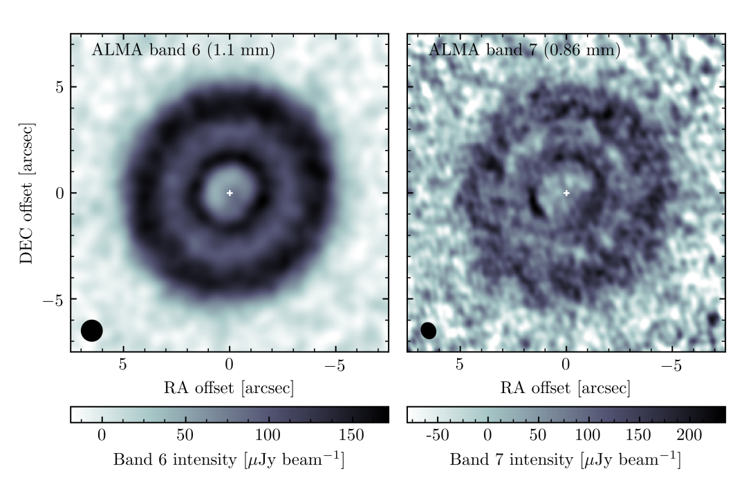
Continuum maps at band 6 and 7 are created using the clean task in CASA 4.7 (McMullin et al., 2007) and are presented in Figure 1. We adopt natural weighting for band 6 and 7 (12m+ACA combined) for a higher signal to noise. These maps have a rms of 6.3 and 27 Jy beam-1 at the center, which increases towards the edges as the maps are corrected by the primary beam, reaching values of 7.0 and 34 Jy beam-1 at (140 au) for band 6 and 7, respectively. The band 6 and band 7 synthesised beams have dimensions of and 222Note that the rms and beam sizes are different to the one reported in Table 1 as the imaging is done with natural weights to increase the S/N, respectively, reaching an approximate resolution of 22 au for band 6 and 15 au for band 7. The higher resolution and sensitivity of these new data reveal a nearly axisymmetric broad disc with a large decrease or gap in the surface brightness centered at a radius of au as suggested by Ricci et al. (2015a). The disc extends from nearly to 180 au, being one of the widest discs resolved at millimetre wavelengths (Matrà et al., 2018a). We compute the total flux by integrating the disc emission inside an elliptical mask with a 180 au semi-major axis and the same aspect ratio as the disc (see §3.1). We find a total flux of and mJy at 1.1 and 0.86 mm (including 10% absolute flux uncertainties), leading to a spatially unresolved millimetre spectral index of , consistent with results from Ricci et al. (2015b) which combined ALMA and ATCA observations. The total flux in band 6 is consistent with that measured by Ricci et al. (2015a) at similar wavelengths and using a more compact ALMA configuration, thus proving that our band 6 observations do not suffer from flux loss or miss large scale structure.
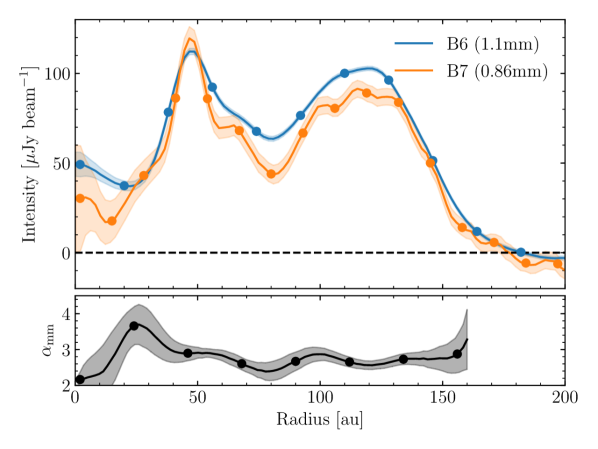
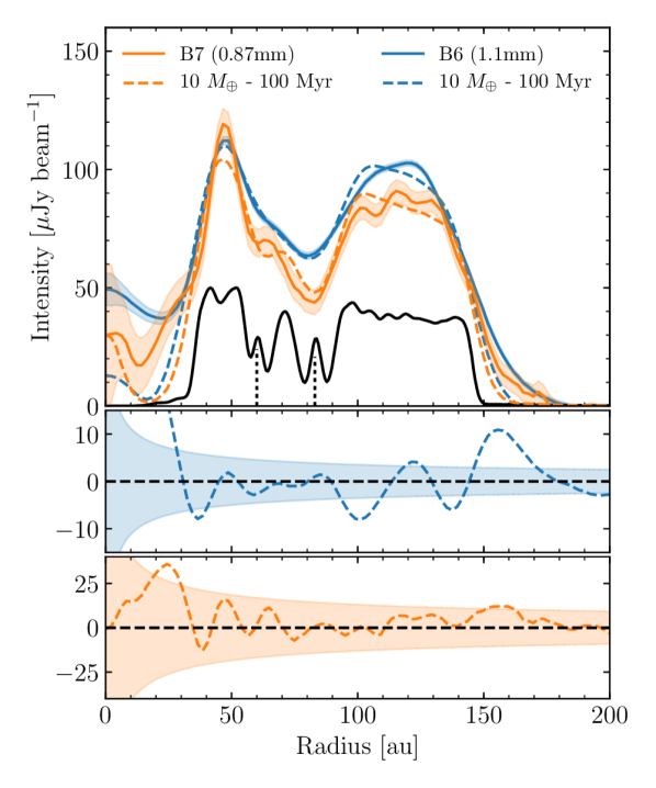
In order to study in more detail the disc radial structure, the top panel of Figure 2 shows the radial intensity profile, computed by azimuthally averaging the disc emission over ellipses as in Marino et al. (2016, 2017a, 2017b). Both in band 6 and 7, we find that the disc surface brightness peaks near the disc inner edge at au, from which it decreases reaching a minimum at 80 au that is deeper in the band 7 profile likely due to the higher resolution. Beyond this minimum, the surface brightness increases until 120 au where it peaks and then decreases steeply with radius. No significant positive emission is recovered beyond 180 au. Within the gap, we find that the radial profile is not symmetric with respect to the minimum, with the outer section (80-100 au) having a steeper slope than the inner part (60-80 au), a feature that is present both in band 6 and 7 data. This is also visible in Figure 1 and is an important feature that could shed light on the origin of this gap. We also compute a spectral index map using multi-frequency clean (nterms=2) and natural weights. The bottom panel of Figure 2 shows the azimuthally averaged radial profile of the spectral index (). From 40 to 150 au the disc has spectral index of roughly (assuming is constant over radii), consistent with the overall spectral index estimated above. Note that uncertainties on do not include the 10% absolute flux uncertainties as we are only interested in relative differences as a function of radius.
In addition to the outer disc, we detect emission from within 30 au that peaks near the stellar position in the azimuthally averaged profile. However, it has a much higher level than the photospheric emission if we extrapolate this from available photometry at wavelengths shorter than 10m using a Rayleigh-Jeans spectral index ( and Jy at 0.86 and 1.1 mm, respectively). Moreover, between 20 and 30 au we also find that has a peak of , although still within from the average spectral index. In §3.1 we recover this inner component in more detail after subtracting the disc emission using a parametric model and we find that it is inconsistent with point source emission, it is significantly offset from the stellar position, and unlikely to be a background sub-millimetre galaxy.
The fact that the disc emission is consistent with being axisymmetric disfavours the scenario in which a planet is scattered out from the inner regions opening a gap through secular interactions with the disc (Pearce & Wyatt, 2015, see their figure 6). In their model, spiral density features are present in the planetesimal disc for hundreds of Myr, which should be imprinted in the mm-sized dust distribution as well, thus being detectable by our observations. In §3.1 we fit parametric models to the data to study with more detail the level of axisymmetry of HD 107146’s disc. Moreover, in §3.2 we compare our observations with N-body simulations of a planet on a circular orbit clearing a gap in a planetesimal disc.
2.2 CO J=3-2 and HCN J=4-3
Despite the increasing number of CO gas detections in nearby debris discs (e.g. Dent et al., 2014; Moór et al., 2015; Marino et al., 2016, 2017a; Lieman-Sifry et al., 2016; Matrà et al., 2017b; Moór et al., 2017), no CO v=0 J=3-2 emission is detected around HD 107146 in the dirty continuum-subtracted data cube. This non detection is, however, not surprising since HD 107146 is significantly older and fainter than the other systems in which primordial gas has been found (i.e. the hybrid discs). Furthermore, the sensitivity of these observations is expected to be insufficient to detect CO gas if being released through collisions of volatile-rich planetesimals (Kral et al., 2017). We search more carefully for CO emission by applying a matched filter technique (Matrà et al., 2015; Marino et al., 2016, 2017a; Matrà et al., 2017b) in which we integrate the emission over an elliptic mask with the same orientation as the disc on the sky (see §3), but in each spatial pixel we integrate only over those frequencies (i.e. radial velocities) where line emission is expected taking into account the Doppler shift due to Keplerian rotation. For this, we assume a stellar mass of 1 , inclination of , PA of , and deprojected minimum and maximum radii of 40 and 150 au, respectively. Using this method we obtain an integrated line flux upper limit of 74 mJy km s-1. Note that we consider the two possible directions of the rotation, obtaining similar limits. We also search for emission that could be present at a specific radius by integrating the emission azimuthally, however no significant emission is found. In §4.5, we use this total flux upper limit to estimate an upper limit on the CO gas mass that could be present in the disc.
Similarly, we search for HCN emission, finding no significant emission. Based on this non detection we place a upper limit of 91 mJy km s-1, which we also use in §4.5 to constrain its abundance in planetesimals in this system. HCN is of particular interest for exocometary studies as, besides being abundant in Solar System comets (Mumma & Charnley, 2011), it has recently been suggested that it could play a key role for prebiotic chemistry in habitable planets (Patel et al., 2015; Sutherland, 2017).
3 Modelling
In this section we model the data using parametric models to constrain the density distribution of solids in the system (§3.1), and N-body simulations of a planet embedded in a planetesimal disc tailored to HD 107146 to constrain the mass and orbit of a putative planet carving the observed gap (§3.2). In both approaches we model the central star as a G2V type star with a mass of 1 , an effective temperature of 5750 K and a radius of 1 .
3.1 Parametric model
We first use a set of parametric models to study the underlying density distribution of mm-sized dust in the system, which we fit directly to the observed visibilities as in Marino et al. (2016, 2017a, 2017b). Inspired by the radial profile of the dust emission (Figure 2), we first choose as a disc model an axisymmetric disc with a surface density that is parametrized as a triple power law that divides the disc into an inner edge, an intermediate section (where the bulk of the dust mass is) and an outer edge. On top of this, the triple power law surface density distribution has a gap, which we parametrise with a Gaussian profile, to reproduce the depression seen in the ALMA data. This parametrization introduces a total of 9 parameters that define the surface density as follows,
| (1) | |||||
| (2) |
where and are the inner and outer radii of the disc, determine how the surface density varies interior to the disc inner radius, within the disc and beyond the disc outer radius. The gap is parametrized with a fractional depth , a center and a full width half maximum (FWHM) . We leave as a free parameter the total dust mass , which is the surface integral of . Although the disc is close to face on, we still model the dust distribution in three dimensions adding the scale height as an extra parameter (i.e. vertical standard deviation of ), and imposing a prior of .
We solve for the dust equilibrium temperature and compute images at 0.86 and 1.13 mm using RADMC-3D333http://www.ita.uni-heidelberg.de/ dullemond/software/radmc-3d/. We assume a weighted mean dust opacity corresponding to dust grains made of a mix of astrosilicates (Draine, 2003), amorphous carbon and water ice (Li & Greenberg, 1998), with mass fractions of 70%, 15% and 15%, respectively, and assuming a size distribution with an exponent of -3.5 and minimum and maximum sizes of 1m and 1cm. This translates to a dust opacity of 1.5 cm2 g-1 at 1.1 mm. We note that these choices in dust composition and size distribution have no significant effect on our modeling apart from the derived total dust mass. We then use these images to compute model visibilities at the same uv points as the 12m band 6, 12m band 7 and ACA band 7 observations by taking the Fast Fourier Transform after multiplying the images by the corresponding primary beam. Additionally, we leave as free parameters the disc inclination (), position angle (PA), RA and Dec offsets for the three observation sets, and a disc spectral index () that sets the flux at 0.86 mm given the dust mass and opacity at 1.1 mm, i.e. the size distribution is assumed to be the same throughout the disc. In total, our model has 19 parameters, 10 for the density distribution and 9 for the disc centre, orientation, and spectral index.
To find the best fit parameters we sample the parameter space using the PYTHON module emcee, which implements Goodman & Weare’s Affine Invariant MCMC Ensemble sampler (Goodman & Weare, 2010; Foreman-Mackey et al., 2013). The posterior probability distribution is defined as the product of the likelihood function (proportional to ) and prior distributions which we assume uniform, although we impose a lower limit for of 0.03 due to model resolution constraints. In computing the over the three visibility sets we applied three constant re-weighting factors for band 6, 12m band 7 and for ACA band 7 that ensures that the final reduced of each of the three sets is approximately 1 without affecting the relative weights within each of these data sets that are provided by ALMA. The re-scaling is necessary as the absolute uncertainty of ALMA visibilities can be offset by a factor of a few, even after re-weighting the visibilities with the task statwt in CASA 4.7. These factors could be alternatively left as free parameters by adding an extra term to the likelihood function, however we find no differences in our results compared to leaving them fixed during multiple tries. Therefore we opt for leaving them fixed.
| Parameter | best fit value | description |
| 3-power law + Gaussian gap | ||
| [] | total dust mass | |
| [au] | disc inner radius | |
| [au] | disc outer radius | |
| inner edge’s slope | ||
| disc slope | ||
| outer edge’s slope | ||
| [au] | radius of the gap | |
| [au] | FWHM of the gap | |
| fractional depth of the gap | ||
| scale height | ||
| PA [] | disc PA | |
| [] | disc inclination from face-on | |
| millimetre spectral index | ||
| Step gap | ||
| [au] | radius of the gap | |
| [au] | width of the gap | |
| depth of the gap | ||
| Eccentric disc | ||
| <0.03 | disc global eccentricity | |
| Inner component | ||
| [au] | disc inner radius | |
| inner edge’s slope | ||
| disc slope | ||
| [au] | radius of the gap | |
| [au] | FWHM of the gap | |
| fractional depth of the gap | ||
| [] | dust mass inner component | |
| [au] | radius of inner component | |
| [au] | radial width of inner component | |
| [] | PA of inner component south of disc PA, | |
| and in the disc plane | ||
| [] | azimuthal width of inner component | |
In Table 2 we present the best fit parameters of our 3-power law model with a Gaussian gap. We find a disc inner radius of 47 au that is significantly larger than the inner edge of au derived by Ricci et al. (2015a). This is because in their model they considered a sharp inner edge, while in ours we allow for the presence of dust within this inner radius, but decreasing towards smaller radii. We find that matches well the radius at which the surface density peaks as seen in Figure 2. Similarly, our estimate of the outer radius (136 au) is significantly smaller than their outer edge (150 au). We find that the disc inner edge has a power law index (slope hereafter) of , while the outer edge is much steeper with a slope of . The intermediate component has a very flat slope of , flatter than the previous estimate (0.59), although the difference could be simply due to different parametrizations, i.e. considering a three vs a single power law parametrization or leaving the gap’s depth as a free parameter vs fixed to 1. Note that the slope derived from the intermediate component does not imply that the mass surface density of planetesimals is flat. In fact, from collisional evolution models we expect the surface density of mm-sized dust and optical depth to have a lower slope than the total mass surface density in regions of the disc where the largest planetesimals are not yet in collisional equilibrium (i.e. have a lifetime longer than the age of the system, Schüppler et al., 2016; Marino et al., 2017b; Geiler & Krivov, 2017). Moreover, we also expect that in the inner regions where the largest planetesimals are in collisional equilibrium, the surface density of material should have a slope close to (Wyatt et al., 2007; Kennedy & Wyatt, 2010), as we find interior to . This suggests that the regions interior to 47 au might be relatively depleted of solids simply due to collisional evolution rather than clearing by planets or inefficient planetesimal formation. We compare the derived inner radius and surface density of millimetre grains ( M⊕ au-2 at 50 au) with collisional evolution models by Marino et al. (2017b), which include how the size distribution evolves at different radii, to estimate the maximum planetesimal size and initial total surface density of solids. We find that the best match has a maximum planetesimal size of km and an initial disc surface density of 0.015 M⊕ au-2 at 50 au, i.e. 5 times the surface density of the Minimum Mass Solar Nebula (Weidenschilling, 1977; Hayashi, 1981) extrapolated to large radii, or a total solid disc mass of 300 M⊕. This implies a very massive initial disc and efficient planetesimal formation at large radii. These conclusions assume, however, that the observed structure in the surface brightness profile arise from collisional evolution neglecting alternative origins. Finally, regarding the disc orientation, we find values that are consistent with previous estimates, but with tighter constraints (see Table 2).
Our results show that the gap is centered at au, consistent with the previous estimate. However, we find a FWHM of 40 au that is much larger than the previous estimate of 9 au, likely due to Ricci et al. (2015a) assuming a gap depth of 100%. Instead, we fit the depth of the gap finding a best fit value of 0.5. We also fit an alternative model in which the gap is a step function with a constant depth, finding best fit values that are similar to the model with the Gaussian gap (see Table 2). The difference in widths between the previous study and this work is interesting as Ricci et al. (2015a) derived the mass of a putative planet clearing a gap in the disc based on the gap’s width and assuming that it should be roughly equal to the planet’s chaotic zone. A 3-4 times wider gap would imply a much higher planet mass as the width of the chaotic zone scales as (Wisdom, 1980; Duncan et al., 1989). Such planet mass estimates assume that the system is in steady state, that the gap is devoid of material, and that the gap’s width is simply equal to the chaotic zone’s width. However, given the age of the system (80-200 Myr), and that any planet may be younger, it is reasonable to consider that the distribution of particles in the planet’s vicinity could still be evolving. Therefore, instead of using the gap’s width to estimate a planet mass, in §3.2 we estimate this by comparing with N-body simulations tailored to HD 107146.

Using the best fit PA and we deproject the observed visibilities and bin them to compare them with our axisymmetric model in Figure 3 (continuous line). The 12m and ACA band 7 observations are consistent with each other within errors, with some systematic differences due to the different primary beams. We find that our best fit model fits well both the real and imaginary components, with the imaginary part being consistent with zero as expected for an axisymmetric disc. However, we find a significant deviation between the real components of the 12m band 7 data and model at around 50 k (corresponding to an angular scale of ), with the model visibility predicting a slightly lower value than the data. This could be due to large scale variations in the spectral index as the same model fits well those baselines in the band 6 data. This deviation is the same when comparing the model with a step gap, which has an indistinguishable visibility profile for baselines shorter than 200 k. Beyond 150 k we also find deviations between the data and model, expected since as shown in Figure 2 the radial profile seems to have structure that is more complex than a simple Gaussian gap.
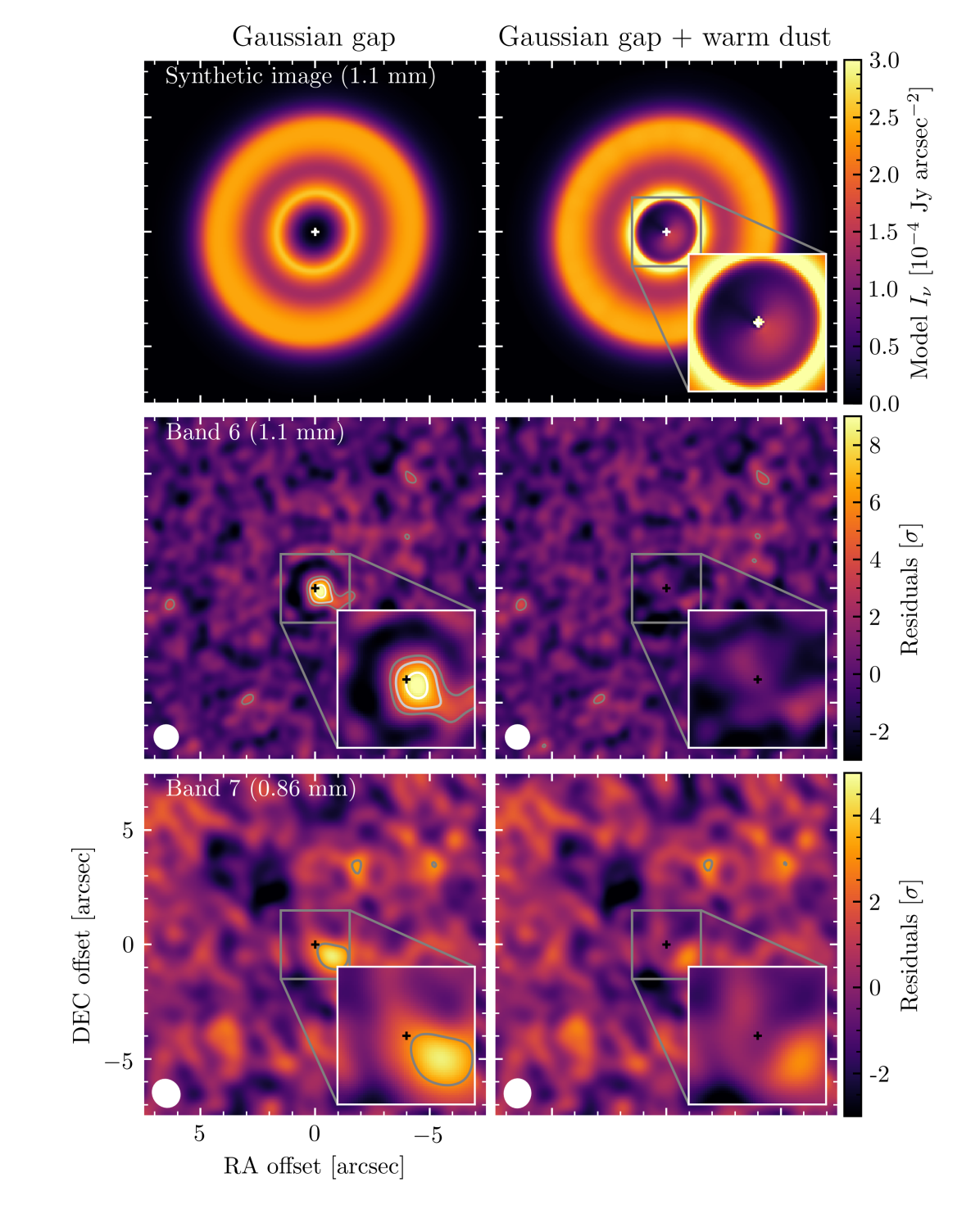
A more intuitive way to study the goodness of fit of our model is to look at the dirty map of the residuals. The left column of Figure 4 shows the dirty maps of the residuals after subtracting our best fit model from the data (in visibility space). These are computed using natural weights, plus an outer taper of for band 7 to obtain a synthesised beam of similar size compared to the band 6 beam. Both band 6 and 7 residual images show significant residuals (with peaks of 9 and 5 times the rms) within the disc inner edge and with a peak that is significantly offset from the stellar position by , corresponding to a projected distance of au. Moreover, the emission is marginally resolved, extending radially by more than a beam (i.e. larger than 10 au) and with an integrated flux significantly higher than the predicted photospheric emission at these wavelengths assuming a Rayleigh-Jeans spectral index (18 and 32 Jy at 1.1 and 0.86 mm). We estimate the flux of these components by integrating the dirty maps over a circular region of diameter, finding an integrated flux of Jy and Jy at 1.1 and 0.86 mm, respectively (without including 10% absolute flux uncertainties). Because this inner emission is resolved, it cannot arise from a compact source such as a planet or circumplanetary material.
We identify two plausible origins for this inner component. It could be the same warm dust that was inferred based on Spitzer data (Morales et al., 2011), as the clump is at a radial distance that is consistent with the inferred black body radius (5-15 au) from its spectral energy distribution (SED), although our detection would imply that the warm component has an asymmetric distribution (see discussion in §4.4). On the other hand, the residual could be also due to a background sub-millimeter galaxy that are often detected incidentally as part of ALMA deep observations (see Simpson et al., 2015; Carniani et al., 2015; Marino et al., 2017b; Su et al., 2017). Sub-millimeter galaxies have typical sizes of the order of 1″ and spectral indices ranging between at mm-wavelengths, thus consistent with the observed clump. We estimate a probability of of finding a sub-millimeter galaxy as bright as 0.3 mJy at 0.86 mm or 0.1 mJy at 1.1 mm, respectively, within the entire band 6 and 7 primary beams (Simpson et al., 2015; Carniani et al., 2015). Hence, the detection of such a bright background object is not a rare event. However, we find that the probability of finding such a bright sub-millimeter galaxy at 0.86 mm and 1.1 mm and co-located with warm dust (i.e within from the star) is only 0.6% and 1%, respectively; therefore favouring the warm dust scenario. In fact, we do not detect any other compact emission above within the band 7 and 6 primary beams, consistent with the number counts of sub-millimeter galaxies. We also discard that this emission could originate from the galaxy detected using HST in 2004, 2005 and 2011 (Ardila et al., 2004; Ertel et al., 2011; Schneider et al., 2014), as its position would only have changed by , and therefore still lie at ( au) from the star in 2017, and is not detected in our observations.
3.1.1 Disc global eccentricity
As shown by Pearce & Wyatt (2014, 2015), a planet on an eccentric orbit can force an eccentricity in a disc of planetesimals through secular interactions. Here we aim to assess if HD 107146’s debris disc could have a global eccentricity and pericentre, using the same parametrization as in Marino et al. (2017a), i.e. taking into account the expected apocentre glow (Pan et al., 2016). We find that the disc is consistent with being axisymmetric, with a 2 upper limit of 0.03 for the forced eccentricity. We find though that the marginalised distribution of peaks at 0.02 with a pericentre that is opposite to the residual inner clump. This peak is likely produced as the residuals are lower when the disc is eccentric and with an apocentre oriented towards the clump’s position angle due to apocentre glow. We therefore conclude that the fit is biased by the inner clump and that the disc is probably not truly eccentric.
3.1.2 Inner component
In order to constrain the geometry or distribution of the inner emission found in the residuals, we add an extra inner component by introducing five additional parameters to our reference parametric model (3-power law surface density with a Gaussian gap). We parametrise its surface density as a 2D Gaussian in polar coordinates, with a total dust mass and centered at a radius and azimuthal angle (measured in the plane of the disc from the disc PA and increasing in an anti-clockwise direction). The width of this Gaussian is parametrized with a radial FWHM and an azimuthal standard deviation . Best fit values are presented in Table 2. We find that this inner component is extended both radially and azimuthally, but concentrated around au and orthogonal to the disc PA (), as we found in the residuals of our axisymmetric model. In the right panel of Figure 4 we present the model image of the best fit model and its residuals, which are below in both band 6 and 7 within the disc inner edge. We also find that the total dust mass of this inner component is M⊕ (1% of the outer disc mass).
When adding this extra inner component we find that the slope of the inner edge is steeper and the inner radius smaller compared with our previous model (symmetric disc model hereafter), as it was probably compensating for the emission within 30 au with a less steep inner edge. We also find a slightly smaller gap radius of 72 au, a larger and deeper gap (51 au wide and 0.58 deep), and a flatter surface density slope of . These differences in the gap’s structure and disc slope are overall consistent within with our previous estimates, but significantly improve the fit at large baselines as Figure 3 shows (dashed blue and orange lines). These improvements in the fit at large baselines are not due to the addition of the clump, but due to the different best fit surface density profile of the outer disc. In fact, the visibilities of the inner component are negligible beyond 200 k. The rest of the parameters are consistent within with the values presented for the symmetric disc model. To have a better estimate of the flux of this inner component, we subtract the new best fit of the outer component (its inner edge is steeper), finding an integrated flux over a circular region of diameter of and mJy at 0.86 and 1.1 mm, respectively (including 10% absolute flux uncertainties)444We also measured the integrated flux of the inner component using the task uvmodelfit in CASA 4.7, obtaining values of and mJy at 1.1 and 0.86 mm, respectively.. Note that this flux is a factor two higher than that estimated from the residuals of the symmetric disc model, as without the inner component the model tries to compensate for the emission interior to 40 au. From these fluxes we estimate a spectral index of , thus still consistent with the typical observed spectral indices of debris discs. Based on this new flux estimate at 0.86 mm, we find an even lower probability of 0.1% and 0.3% of finding a sub-mm galaxy as bright as this inner emission at 0.86 and 1.1 mm, respectively, and within from the star (Simpson et al., 2015; Carniani et al., 2015). These results also confirm that the peak of this inner component is significantly offset from the star and it is incompatible with an axisymmetric inner component. If this emission is produced by warm dust, then it could bring valuable insights into the origin of warm dust emission in general, as it is inconsistent with an axisymmetric asteroid belt (see §4.4).
Because the new estimate of the inner edge slope is too steep to be consistent with being set by collisional evolution, the maximum planetesimal size is only constrained to be km. Despite this, the relative brightness between the inner and outer components can still be explained simply by collisional evolution. This has also been found for other systems with warm dust components, e.g. q1 Eridani (Schüppler et al., 2016), suggesting the presence of planets clearing the material in between (Shannon et al., 2016).
3.2 N-body simulations
In this section we compare the observations with dynamical N-body simulations of a planet embedded in a planetesimal disc. To simulate the gravitational interactions between the planet and particles we use the N-body software package REBOUND (Rein & Liu, 2012), using the hybrid integrator Mercurius555We also used Hermes in several trial runs; however, we decided to use Mercurius instead because with Hermes we obtained results that differ significantly from other integrators such as ias15, whfast and the hybrid integrator within Mercury. We found that some particles outside the chaotic zone were driven to unstable orbits and did not conserve their Tisserand parameter. The possibility of a potential bug in Hermes was confirmed by private communication with Hanno Rein. that switches from a fixed to a variable time-step when a particle is within a given distance from the planet (here chosen to be 8 Hill radii). The fixed time step is chosen to be 4% of the planet’s period, which is lower than 17% of the orbital period of all particles in the simulation. Although the total mass of the disc could be tens of M⊕, and thus comparable with the mass of the simulated planets, we assume particles have zero or a negligible mass. In §4.3 we discuss the effect of considering a massive planetesimal disc on planet disc interactions.
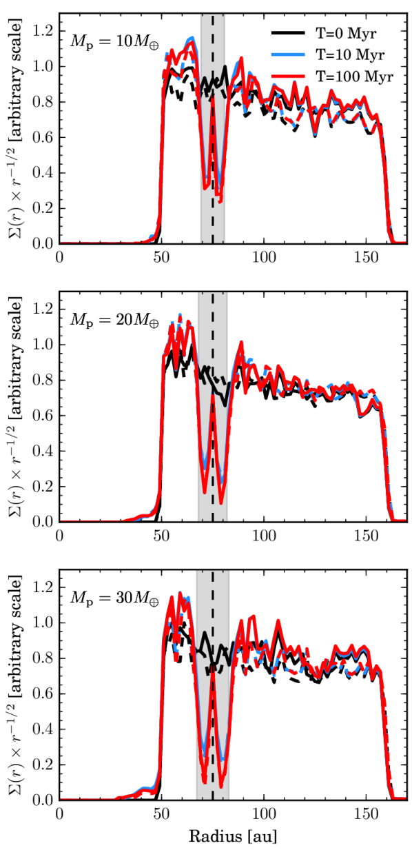
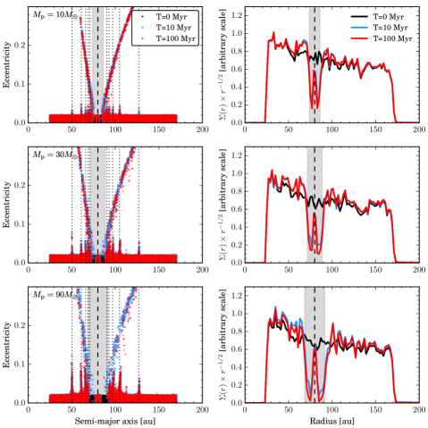
Particles are initially randomly distributed in the system with a uniform distribution in semi-major axis () between 20 and 170 au (i.e. with a surface density proportional to ), with an eccentricity and inclination uniformly distributed between 0-0.02 and 0-0.01 radians, respectively. We use a total number of particles, sufficient to sample the 150 au span in semi-major axes and recover smooth images of the disc density distribution. The planet is placed on a circular orbit at 80 au and assumed to have a bulk density of 1.64 g cm-3 (Neptune’s density). We integrate the evolution of the system up to 200 Myr, roughly the upper limit for the age of the system. We run a set of simulations with planet masses varying from 10 to 100 with a 5 spacing.
In order to translate the outcome of these simulations to density distributions used to produce synthetic images, we populate the orbits of each particle with 200 points randomly distributed uniformly in mean anomaly as in Pearce & Wyatt (2014), but in the frame co-rotating with the planet in order to see if there are resonant structures (e.g. loops or Trojan regions). We find however no significant azimuthal structures due to first or second order resonances in the derived surface density of particles. We weight the mass of each particle based on its initial semi-major axis to impose an initial surface density proportional to between a minimum and maximum semi-major axis (). Finally, because we only run simulations with a fixed planet semi-major axis of 80 au to save computational time, we scale all the distances in the output of the simulation and leave as a free parameter (only varying roughly between 75-80 au). This linear scaling is motivated by the fact that some of the features that we are interested in should scale with semi-major axis (e.g. Hill radius, mean-motion resonances, chaotic zone), although some other important quantities, such as the scattering diffusion timescale (Tremaine, 1993), have a dependency on that is different from linear. In Appendix A we test the validity of the scaling approximation for the narrow range of planet semi-major axis that we explore.
In Figure 5 we present, as an example, the evolution of , and the surface density of particles for planet masses of 10, 30 and 90 M⊕. The width of the chaotic zone is overlayed in grey (note that this is a region in semi-major axis rather than radius), to compare with the gap in the surface density cleared by the planet. Although by 100 Myr the chaotic zone is almost empty of material (except for particles in the co-rotation zone) the surface density is not zero inside the gap as some particles have apocentres or pericentres within this region while being scattered by the planet. Some particles also remain on stable tadpole or Trojan orbits until the end of the simulation, creating an overdensity within the gap at 80 au. Interior and exterior to the planet, a small fraction of particles are in mean motion resonance with the planet and have their eccentricities increased. In agreement with previous work, we find that the gap’s width approximates to the chaotic zone, and its width does not vary after 10 Myr for the planet masses explored.
To compare with observations, we use snapshots of the simulations at 50, 100 and 200 Myr since the age of the system is uncertain and could vary roughly within this range. These ages assume that the putative planet formed (or grew to its current mass) early during the evolution of this system, rather than recently, or that this is the time since the planet formed. For each assumed epoch, we explore the parameter space using the same MCMC technique as in §3.1, varying and , the surface density exponent , the semi-major axis of the planet, and its mass by interpolating the resulting surface density between two neighbouring simulations. We also leave as free parameters the disc orientation, pointing offsets and spectral index, and instead of varying the disc scale height we assume a flat disc. We find a best fit mass of M⊕ and semi-major axis of au, independently of the assumed age since after 10 Myr there is no significant evolution in the orbits of particles near the planet (see Figure 5). We find, however, that our best fit cannot reproduce well the width and depth of the gap. This is illustrated in the top and middle panels in Figure 6, where the model has a narrower gap compared with the band 6 radial profile, and thus overall larger residuals. Although larger planet masses could produce wider gaps, these would also be significantly deeper and thus inconsistent with the observations. Moreover, the planet gap could be even deeper if, for example, we assume a different starting condition with a depleted surface density within the planet’s feeding zone as it accreted a large fraction of that material while growing. To test this, we repeat the fitting procedure, but removing those particles that start the simulation within two Hill radii from the planet’s orbit (planet’s feeding zone). We find a slightly lower best fit planet mass of M⊕, but overall the fit is worse with a difference of in the total , strongly preferring the model with particles starting near the planet. Therefore, we conclude that a single planet on a circular orbit that was born within the outer disc is unable to explain the ALMA observations.

4 Discussion
4.1 The gap’s origin
As discussed in §1, we identify multiple scenarios where a single planet might open a gap in a planetesimal disc. Below we discuss these and how well they could fit the data.
4.1.1 Single planet on a circular orbit
As we showed in §3.2, a single planet on a circular orbit and formed inside the gap could clear its orbit of debris through scattering, opening a gap with a width similar to the chaotic zone. Such a planet, however, needs to be very massive to produce a au wide gap ( MJup), which, on the other hand, results in a gap that is significantly deeper than our observations suggest. Based on these constraints we find that a 30 M⊕ planet is the best trade-of between the gap’s width and depth.
If, however, the planet could migrate (inwards or outwards) then these two observables could become compatible. A low mass planet that migrated through the disc could carve a sufficiently wide gap to explain the au gap’s width. Migration could also explain the relative depth of that is observed as after migrating, the planet would also leave behind debris that was scattered onto excited orbits, but that do no longer cross the planet’s orbit (e.g. Kirsh et al., 2009), therefore the gap would still contain a significant fraction of the original material. Planet migration could be induced by planetesimal scattering, which is discussed in §4.3.
4.1.2 Multiple planets on circular orbits
If we assume planet migration is negligible (e.g. disc mass around the planet’s orbit is much lower than its mass), then multiple planets would need to be present to carve such a wide and shallow gap. Let us assume that the gap was carved by multiple equal mass planets orbiting between 60 and 90 au. As shown by Shannon et al. (2016) and in §3.2, the width of the gap and age of the system place tight constraints on the minimum mass of a planet to clear the region surrounding its orbit, and on the maximum number of planets that could be orbiting within the gap based on a stability criterion. Given HD 107146’s age limits of and 200 Myr, only planets with masses greater than 10 M⊕ would have enough time to clear their orbits via scattering. On the other hand, only planet masses M⊕ can create a gap that is not too deep compared with our observations. Given this range of planet masses, we estimate that a maximum of three 10 M⊕ planets could orbit between 60 and 90 au spaced by 8 mutual Hill radii at the limits of long term stability (Chambers et al., 1996; Smith & Lissauer, 2009). If we require planets to be spaced by more than 8 mutual Hill radii, this multiplicity reduces considerably to two or only one planet if planet masses are slightly higher. We tested this by running new simulations with the same parameters as in §3.2, but instead with a pair of 30 or 10 M⊕ planets and semi-major axes ranging between 60 to 90 au. After a few iterations we found a good fit using two 10 M⊕ planets with semi-major axes of 60 and 83 au (i.e. spaced by 12 Mutual Hill radii). Figure 7 shows the radial profile for this model reproducing the width and depth of the gap. The relative depth of the gap is similar to the one observed as there are still particles on stable orbits at around 70 au and trapped in the co-orbital regions of the two planets — note that there are residuals above at the inner and outer edge of the disc because this model has sharp boundaries in semi-major axis. If we assumed that no particles were present near the planet at the start of the simulation as commented in §3.2, then even lower mass planets creating narrower gaps would be needed in order to achieve an overall gap depth of 50%.
4.1.3 Planet(s) on eccentric orbits
Although a single or multiple low mass planets might explain the observed gap, the formation of an ice giant planet at au encounters significant difficulties compared to within a few tens of au (see §4.2). The scenario proposed by Pearce & Wyatt (2015), where a planet opens a broad gap through secular interactions, circumvents some of these problems as the planet is formed closer in at 10-20 au, and scattered out by a more massive planet onto an eccentric orbit with a larger semi-major axis. This scenario was able to fit the mean radial profile derived by Ricci et al. (2015a) and predicted the presence of asymmetries in the form of spiral features and a small offset between the inner and outer regions of the disc due to secular interactions with the planet. However, no significant offset between the inner and outer regions is present in our observations. By fitting an ellipse to the inner and outer bright arcs in the band 6 image (roughly at 50 and 110 au), we constrain the offset to be , (i.e. consistent with zero and lower than 1.6 au). This translates to a maximum eccentricity of 0.03 if we assume that the outer bright arc is circular while the inner arc is eccentric and thus offset from the star. Moreover, our observations suggest that the disc inner edge is much steeper than predicted by Pearce & Wyatt (2015), thus inconsistent with their model. A last recently proposed scenario involves two interior planets with low but non-zero eccentricity, which open a gap in the outer regions due to secular resonances (see Yelverton et al., in prep). Although this scenario can produce an observable gap, in its simplest form the model produces a gap that is narrower than seen for HD 107146.
4.1.4 Dust-gas interactions
There are other scenarios that might not require the presence of planets to produce a gap or multiple ring structures in the dust distribution. Photoelectric instability (Klahr & Lin, 2005; Besla & Wu, 2007; Lyra & Kuchner, 2013; Richert et al., 2017) is one of those scenarios and has received particular attention lately as the presence of vast amounts of gas around a few debris discs suggests that this mechanism might be common. However, this mechanism is only important when dust-to-gas ratios are comparable and it is not yet clear if relevant for the dust distribution of large millimetre-sized grains that are not well coupled to the gas. Assuming some residual primordial gas could still be present in the disc, we convert our CO gas mass upper limit of M⊕ (see §4.5 below) to a total gas mass upper limit of M⊕ (assuming a CO/H2 ratio of ) or a surface density of g cm-2. This upper limit is comparable to the total dust mass in millimetre grains, thus photoelectric instability could occur. However, using this gas surface density upper limit we estimate a Stokes number of for millimetre grains, thus the stopping time is much longer than the collisional lifetime of millimetre dust and of the order of the age of the system. Therefore, we conclude that photoelectric instability does not play an important role in the formation of the structure observed by ALMA around HD 107146.
4.2 Planet formation at tens of au
Based on these new ALMA observations, if the gap was cleared by a single or multiple planets, these must have a low mass (30 M⊕) and formed between 50 and 100 au. Otherwise, if the planets were formed closer in and scattered out onto an eccentric orbit, the disc would appear asymmetric (Pearce & Wyatt, 2015). Such low planet masses and orbits at tens of au resemble the ice giant planets in the Solar System, but with a semi-major axis 2-3 times larger than Neptune’s. Could such planets have formed in situ as these observations suggest? HD 107146’s broad and massive debris disc indicates that planetesimals efficiently formed at a large range of radii from 40 to 140 au. Moreover, the mass of these putative planets ( M⊕) is consistent with the solid mass available in their feeding zones ( Hill radii wide), based on the dust surface density derived in §3.1 and extrapolating it to the total mass surface density (assuming a size distribution and planetesimals up to sizes of 10 km). Nevertheless, in situ formation encounters the two following problems. First, although a planet at au might grow through pebble accretion fast enough to form an ice giant before gas dispersal (Johansen & Lacerda, 2010; Ormel & Klahr, 2010; Lambrechts & Johansen, 2012; Morbidelli & Nesvorny, 2012; Bitsch et al., 2015), it requires the previous formation of a massive planetesimal (or protoplanet) of M⊕ (so-called transition mass). However, newly born planetesimals through streaming instability (Youdin & Goodman, 2005) have characteristic masses of rather M⊕ (Johansen et al., 2015; Simon et al., 2016). These planetesimals can grow through the accretion of pebbles and smaller planetesimals, but this growth (so-called Bondi accretion) is very slow for low mass bodies at large stellocentric distances (Johansen et al., 2015). A possible solution to this problem is that the protoplanetary disc around HD 107146 was unusually massive and long-lived, which would increase the chances of forming such a protoplanet. Alternatively, the low mass protoplanet could have formed closer in and been scattered out and circularised during the protoplanetary disc phase. The second problem that in-situ formation faces is related to planet migration. A protoplanet growing to form an ice giant is expected to migrate inwards through type-I migration (Tanaka et al., 2002). While this might imply that the single or multiple putative planets might have formed at larger radii, our observations suggest that they would have attained most of their mass within the observed gap, i.e. within 100 au. If pebble accretion is fast enough, the planet could grow fast and migrate only slightly before disc dispersal.
Why would planets form only between 60-90 au within this 100 au wide disc of planetesimals? While no planets might have formed beyond 90 au as planetesimal accretion was too slow for a planetesimal to reach the transition mass and efficiently accrete pebbles, this is not the case for planetesimals formed at smaller radii between the inner edge of the disc and the orbit of the innermost putative planet. Why did only planetesimals form between 40-60 au? Planetesimal growth might have been hindered there if the orbits of large solids were stirred by inner planets, making their accretion rate slower. Alternatively, planetesimal growth between 60-90 au could have been more efficient due to a local enhancement in the available solid mass. As stated before, it is also possible that the low mass protoplanet did not form in situ, but it was scattered out from further in.
4.3 Massive planetesimal disc
Here we discuss the effect that a massive planetesimal disc could have on the conclusions stated above where we assumed a disc of negligible mass ( M⊕). As shown in §3, this debris disc is likely very massive and thus affects the dynamics of this system, e.g. because of the gravitational force on the planet and disc self-gravity. A massive disc can induce planetesimal driven migration where the planet migrates through a planetesimal disc due to the angular momentum exchange in close encounters (e.g. Fernandez & Ip, 1984; Ida et al., 2000; Gomes et al., 2004). This type of migration has been well studied in the context of the outer Solar System, as it could have driven an initially compact orbital configuration to a more extended and current configuration (Hahn & Malhotra, 1999, 2005), or towards an orbital instability (e.g. Tsiganis et al., 2005). In all these models the outer planets scatter material in to Jupiter which ejects most of it, leading to an outward migration of the outer planets and a small inward migration of Jupiter. However, Ida et al. (2000) showed that even in the absence of interior planets self-sustained migration could have led Neptune’s orbit to expand due to the asymmetric planetesimal distribution around it. A more recent work by Kirsh et al. (2009), however, showed that a single planet embedded in a planetesimal disc migrates preferentially inwards due to the timescale difference between the inner and outer feeding zones (see also Ormel et al., 2012). Therefore, we expect that the putative planet at 80 au around HD 107146 is likely migrating or has migrated inwards since it formed.
Simple scaling relations from Ida et al. (2000) predict that the migration rate should be of the order of
| (3) |
which agrees roughly with numerical simulations (e.g. Kirsh et al., 2009). Given the expected surface density of planetesimals at 80 au around HD 107146 ( M⊕ au-2 for a maximum planetesimal size of 10 km), Equation 3 predicts that the migration rate is such that the planet would have crossed the whole disc reaching its inner edge in only a few Myr. Kirsh et al. (2009) found, however, that when the planet mass exceeds that of the planetesimals within a few Hill radii, the migration rate decreases strongly with planet mass. Assuming that the gap is indeed caused by a single or multiple planets between 60-90 au, given the 30 M⊕ upper limit for the planet mass we conclude that the surface density of planetesimals must be much lower than 0.01 M⊕ au-2 to hinder planetesimal driven migration, i.e. a total disc mass M⊕. If not the surface density profile would probably be significantly different without a well defined gap. This dynamical upper limit together with the lower limit derived from collisional models constrain the total disc mass to be between M⊕, which is close to the maximum solid mass available in a protoplanetary disc under standard assumptions (e.g. disc-to-stellar mass ratio of 0.1 and gas-to-dust mass ratio of 100). This particularly high disc mass at the limits of feasibility is not unique, but a confirmation of the so-called “disc mass problem” as many other young and bright discs need similar or even higher masses according to collisional evolution models (see discussion in Krivov et al., 2018).
Although we expect that the gap produced by a migrating planet might look significantly different compared with the no migration scenario (e.g. wider and radially and perhaps azimuthally asymmetric), none of the above studies provided a prediction for the resulting surface density of particles during planetesimal driven migration that we could compare with our observations. In experimental runs with a 10 or 30 M⊕ planet and a similar mass planetesimal disc (using massive test particles) we find that the planet migrates inward 5-40 au in 100 Myr depending on the planet and disc mass, and that the gap has an asymmetric radial profile that is significantly distinct from the no-migration scenario, which could explain why we find a slight asymmetry within the gap (see §2.1). Future comparison with numerical simulations of planetesimal-driven migration could provide evidence for inward or outward migration, and thus set tighter constraints on the disc and planet mass. Dynamical estimates of the disc mass could also shed light on the disc mass problem, confirming the high mass derived from collisional models or rather indicating that these need to be revisited.
4.4 Warm inner dust component
While IR excess detections can be generally explained by a single temperature black body, there is a large number of systems that show evidence for a broad range of temperatures that are hard to explain simply as due to a single dusty narrow belt, even with temperatures varying as a function of grain size (e.g. Backman et al., 2009; Morales et al., 2009; Chen et al., 2009; Ballering et al., 2014; Kennedy & Wyatt, 2014). Although this might be explained by material distributed over a broad range of radii (like in protoplanetary discs), an alternative and very attractive explanation for these systems is the presence of a two-temperature disc, with an inner asteroid belt and an outer exo-Kuiper belt, analogous to the Solar System (e.g. Kennedy & Wyatt, 2014; Schüppler et al., 2016; Geiler & Krivov, 2017). HD 107146 is a good example of this type of system (Ertel et al., 2011; Morales et al., 2011), with a significant excess at 22 m that cannot be reproduced by models of a single outer belt, but rather is indicative of dust located within au produced in an asteroid belt. These type of belts are typically hard to resolve due to the small separation to the star (hindering scattered light observations) where current instruments are not able to resolve and due to their low emissivity that peaks in mid-IR.
Is the detected inner emission related to the m excess? In order to test if the inner emission seen by ALMA is compatible with being warm dust, we use the parametric model developed in §3.1 to see if it can reproduce the available photometry of this system, including the mid-IR excess. We introduce, though, two changes to the model assumptions: first, we modify the size distribution index from -3.5 to -3.36 to be consistent with the derived spectral index in this work and previous studies (Ricci et al., 2015b); and second, we extend the size distribution from 1 to 5 cm. The latter is necessary to reproduce the photometry at 7 mm as the contribution from cm-sized grains is significant at these wavelengths. In Figure 8 we compare the model and observed SED, including the new ALMA photometric points of the inner component. Despite the simplicity of our model, it reproduces successfully both the photometry at 22 m and at millimetre wavelengths, confirming that our detection is consistent with being warm dust emission.

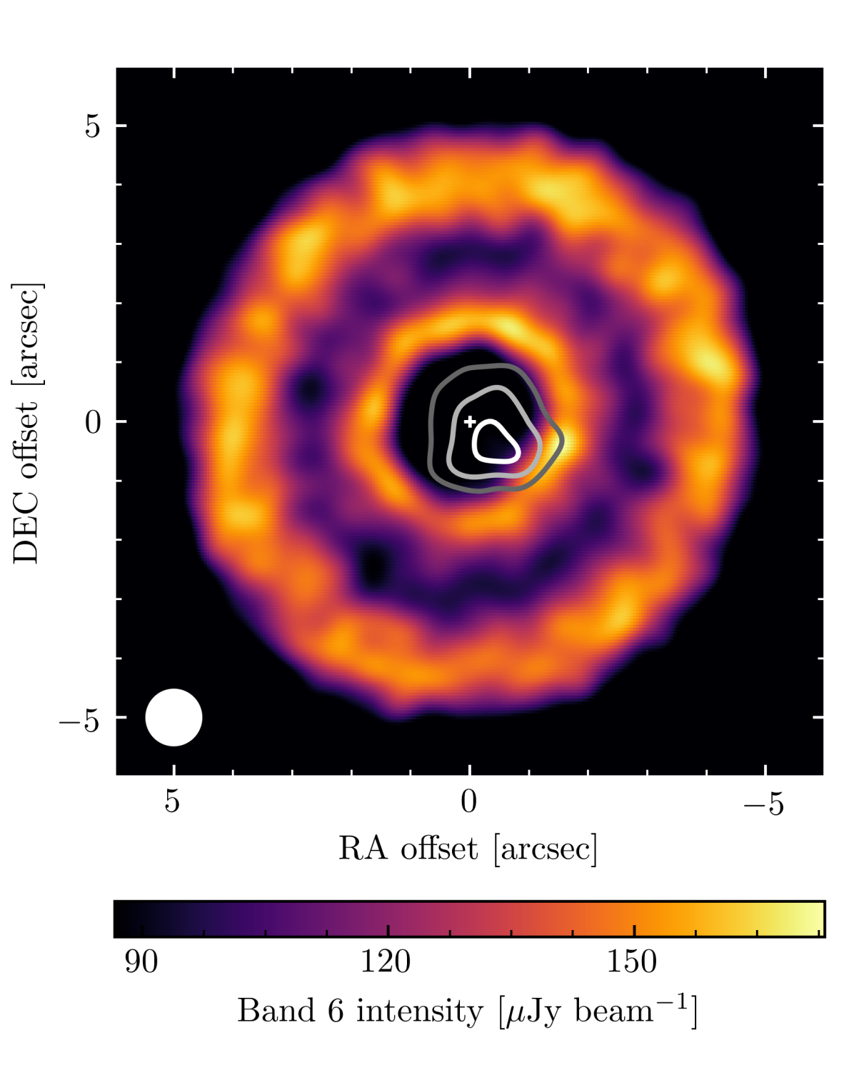
These new ALMA observations provide unique information on the nature of the warm dust emission as it is marginally resolved (see Figure 9). The surface brightness peaks at au, thus roughly in agreement with the predicted location based on SED modelling. The emission, however, is far from originating in an axisymmetric asteroid belt, but is rather asymmetric with a maximum brightness towards the south west side of the disc. What could cause such an asymmetric dust distribution? We identify three scenarios proposed in the literature that could cause long- or short-term brightness asymmetries in a disc or belt.
First, the inner emission could correspond to an eccentric disc, which at millimetre wavelengths would be seen brightest at apocentre. This is known as apocentre glow, which is caused by the increase in dust densities at apocentre for a coherent disc (Wyatt, 2005; Pan et al., 2016). Disc eccentricities can be caused by perturbing planets (e.g. Wyatt et al., 1999; Nesvold et al., 2013; Pearce & Wyatt, 2014), as it has been suggested to explain Fomalhaut’s eccentric debris disc (Quillen, 2006; Chiang et al., 2009; Kalas et al., 2013; Acke et al., 2012; MacGregor et al., 2017) and HD 202628 (Krist et al., 2012; Thilliez & Maddison, 2016; Faramaz et al., in prep). At long wavelengths, the contrast between apocentre and pericentre brightness is expected to be approximately (Pan et al., 2016)
thus to reach a contrast higher than 2 (as observed for HD 107146’s inner disc), the disc eccentricity would need to be higher than 0.5. Assuming the disc eccentricity corresponds to the forced eccentricity (i.e. free eccentricities are much smaller), then the perturbing planet should have a very high eccentricity . One potential problem with this scenario is that the outer disc does not show any hint of being influenced by an eccentric planet. This problem could be circumvented if the true eccentricity of the inner belt is lower than derived based on the image residuals (e.g. ) and the inner planet has a semi-major axis of only a few au, as the forced eccentricity on the outer disc would be much smaller. Alternatively, if the disc or putative outer planet(s) are much more massive than the inner eccentric planet, the disc might remain circular as it is observed.
A second potential scenario relates to a recent collision between planetary embryos, which would release large amounts of dust at the collision point producing an asymmetric dust distribution that could last for orbits or Myr at 20 au (Kral et al., 2013; Jackson et al., 2014). In such a scenario the pinch point would appear brightest since the orbits of the generated debris converge where the impact occurred and more debris is created from collisions. Thus, the pinch point would appear radially narrow. However, both our band 6 and 7 datasets show that the emission is radially broad at its brightest point, spanning au. This could be circumvented if the collision occurred within a broad axisymmetric disc. Higher resolution observations are necessary to discard this scenario or confirm these two inner components.
Finally, a third possible scenario is that the asymmetric structure is caused by planetesimals trapped in mean motion resonances (typically 3:2 and 2:1) with an interior planet that migrated through the planetesimal disc (Wyatt & Dent, 2002; Wyatt, 2003, 2006; Reche et al., 2008). The exact dust spatial distribution depends on the planet mass, migration rate and eccentricity. The single clump inferred from our observations suggests that planetesimals would be trapped predominantly on the 2:1 resonance rather than 3:2 as the latter only creates a two clump symmetric structure. Simulations by Reche et al. (2008) showed that in order to trap planetesimals in the 2:1 resonance, a Saturn mass planet (or higher) with a very low eccentricity was needed, therefore, placing a lower limit on the planet mass if the asymmetry is due to resonant trapping.
Future observations could readily distinguish between scenarios 1-2 and 3, as in the first two scenarios the orientation of the asymmetry should stay constant (precession timescales are orders of magnitude longer than the orbital period), while in the third scenario it should rotate at the same rate as the putative inner planet orbits the star. Moreover, higher resolution and more sensitive observations could reveal if the disc is eccentric, smooth with a radially narrow clump, or smooth with a radially broad clump (scenarios 1 to 3, respectively). Observations at shorter wavelength would also be useful. In the eccentric disc scenario we expect the disc to be eccentric and broader due to radiation pressure on small dust grains, while resonant structure would be completely absent and the disc should look axisymmetric as small grains are not trapped also due to radiation pressure. Finally, future ALMA observations should be able to definitely rule out the possibility of the inner emission arising from a sub-mm galaxy. Given HD 107146’s proper motion (-174 and -148 mas yr-1 in RA and Dec. direction, respectively), we would expect that in 2 years any background object should shift by towards the north east with respect to HD 107146, thus enough to be measured with ALMA observations of similar sensitivity and resolution to the ones presented here.
4.5 Gas non detections
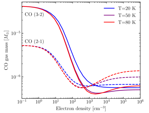
In §2.2 we search for CO and HCN secondary origin gas around HD 107146. Although we did not find any, here we use the flux upper limits, including also the 40 mJy km s-1 upper limit for CO J=2-1 from Ricci et al. (2015a), to derive an exocometary gas mass upper limit in this disc. It has been demonstrated that in the low density environments around debris discs, gas species are not necessarily in local thermal equilibrium (LTE), which typically leads to an underestimation of CO gas masses (Matrà et al., 2015). Here we use the code developed by (Matrà et al., 2018b) to estimate the population of the CO rotational level in non-LTE based on the radiation environment, densities of collisional partners, and also taking into account UV fluorescence. We consider as sources of radiation the star, the CMB and the mean intensity due to dust thermal emission within the disc (calculated using our model and RADMC-3D). We choose 80 au as the representative radius, which is approximately the middle radius of the disc, and left as a free parameter the density of collisional partners (here assumed to be electrons). Based on our model, the dust temperature should roughly vary between 50 to 30 K between the disc inner and outer edge. Figure 10 shows the CO gas mass upper limit as a function of electron density for different kinetic temperatures. We find that for electron densities lower than cm-3, the CO J=2-1 upper limit is more constraining than J=3-2 and vice versa. Overall, the CO gas mass must be lower than M⊕. We then use equation 2 in Matrà et al. (2017b) and the estimated photodissociation timescale of 120 yr to estimate an upper limit on the CO+CO2 mass fraction of planetesimals in the disc, but we find no meaningful constraint because this CO gas mass upper limit is much higher than the predicted M⊕ if gas were released in collisions of comet-like bodies (e.g. Marino et al., 2016; Kral et al., 2017; Matrà et al., 2017a, b).
In the absence of a tool to calculate the population of rotational levels for HCN, we estimate a mass upper limit assuming LTE. For temperatures ranging between 30-50 K, we find an upper limit of M⊕, which translates to an upper limit on the mass fraction of HCN in planetesimals of 3%, an order of magnitude higher than the observed abundance in Solar System comets (Mumma & Charnley, 2011). Note that this HCN upper limit could be much higher due to non-LTE effects, thus this 3% limit must be taken with caution.
5 Conclusions
In this work, we have analysed new ALMA observations of HD 107146’s debris disc at 1.1 and 0.86 mm, to study a possible planet-induced gap suggested by Ricci et al. (2015a) with a higher resolution and sensitivity. These new observations show that HD 107146, a 80-200 Myr old G2V star, is surrounded by a broad disc of planetesimals from 40 to 140 au, that is divided by a gap 40 au wide (FWHM), centered at 80 au and 50% deep, i.e. the gap is not devoid of material. We constrained the disc morphology, mass and spectral index by fitting parametric models to the observed visibilities using an MCMC procedure. We find that the disc is consistent with being axisymmetric, and we constrain the disc eccentricity to be lower than 0.03.
The observed morphology of HD 107146’s debris disc suggests the presence of a planet on a wide circular orbit opening a gap in a planetesimal disc through scattering. We run a set of N-body simulations of a planet embedded in a planetesimal disc that we compare with our observations. We find that the observed morphology is best fit with a planet mass of 30 M⊕, but significant residuals appear after subtracting the best fit model. We conclude that the observed gap cannot be reproduced by the dynamical clearing of such a planet as the gap it creates is significantly deeper and narrower than observed. We discuss that this could be circumvented by allowing the planet to migrate (e.g. due to planetesimal driven migration) or by allowing multiple planets to be present. We discuss how a planet could have formed in situ if the primordial disc was massive and long-lived, and possibly grew to its final mass very quickly and by the end of the disc lifetime (e.g. through pebble accretion), avoiding significant inward migration and runaway gas accretion. Moreover, because the putative planet(s) could undergo very fast planetesimal driven migration, we set an upper limit on the surface density and total mass of the disc.
These ALMA observations also revealed unexpected emission near the star that is best seen when subtracting our best fit parametric model of the outer disc. This inner component has a total flux of 0.8 and 0.3 mJy at 0.86 mm and 1.1 mm, respectively, a peak intensity that is significantly offset from the star by (15 au), and we resolve the emission both radially and azimuthally. Its radial location indicates that it could be the same warm dust that had been inferred to be between 10-15 au to explain HD 107146’s excess at m. Indeed, we fit this emission with an extra inner asymmetric component finding a good match with these ALMA observations and also with HD 107146’s excess at m. We constrain its peak density at 19 au, and a radial width of at least 20 au. We hypothesise that this asymmetric emission could be due to a disc that is eccentric due to interactions with an eccentric inner planet, asymmetric due to a recent giant collision, or clumpy due to resonance trapping with a migrating inner planet. On the other hand, we find that this inner emission is unlikely to be a background sub-mm galaxy, as the probability of finding one as bright as 0.8 mJy at 0.86 mm within the disc inner edge (i.e. co-located with the warm dust) is 0.1%.
Finally, although it had been demonstrated by Ricci et al. (2015a) that no primordial gas is present around HD 107146, we search for CO and HCN gas that could be released from volatile-rich solids throughout the collisional cascade in the outer disc. However, we find no gas, but we place upper limits on the total gas mass and HCN abundance inside planetesimals, being consistent with comet-like composition.
Acknowledgements
We thank Bertram Bitsch for useful discussion on planet formation and pebble accretion. JC and VG acknowledge support from the National Aeronautics and Space Administration under grant No. 15XRP15_20140 issued through the Exoplanets Research Program. MB acknowledges support from the Deutsche Forschungsgemeinschaft (DFG) through project Kr 2164/15-1. VF’s postdoctoral fellowship is supported by the Exoplanet Science Initiative at the Jet Propulsion Laboratory, California Inst. of Technology, under a contract with the National Aeronautics and Space Administration. GMK is supported by the Royal Society as a Royal Society University Research Fellow. LM acknowledges support from the Smithsonian Institution as a Submillimeter Array (SMA) Fellow. This paper makes use of the following ALMA data: ADS/JAO.ALMA#2016.1.00104.S and 2016.1.00195.S. ALMA is a partnership of ESO (representing its member states), NSF (USA) and NINS (Japan), together with NRC (Canada) and NSC and ASIAA (Taiwan) and KASI (Republic of Korea), in cooperation with the Republic of Chile. The Joint ALMA Observatory is operated by ESO, AUI/NRAO and NAOJ. Simulations in this paper made use of the REBOUND code which can be downloaded freely at http://github.com/hannorein/rebound.
References
- Absil et al. (2013) Absil O., et al., 2013, A&A, 555, A104
- Acke et al. (2012) Acke B., et al., 2012, A&A, 540, A125
- Andrews (2015) Andrews S. M., 2015, PASP, 127, 961
- Ardila et al. (2004) Ardila D. R., et al., 2004, ApJ, 617, L147
- Backman et al. (2009) Backman D., et al., 2009, ApJ, 690, 1522
- Ballering et al. (2014) Ballering N. P., Rieke G. H., Gáspár A., 2014, ApJ, 793, 57
- Besla & Wu (2007) Besla G., Wu Y., 2007, ApJ, 655, 528
- Bitsch et al. (2015) Bitsch B., Lambrechts M., Johansen A., 2015, A&A, 582, A112
- Boley (2009) Boley A. C., 2009, ApJ, 695, L53
- Booth et al. (2016) Booth M., et al., 2016, MNRAS, 460, L10
- Boss (1997) Boss A. P., 1997, Science, 276, 1836
- Burns et al. (1979) Burns J. A., Lamy P. L., Soter S., 1979, Icarus, 40, 1
- Carniani et al. (2015) Carniani S., et al., 2015, A&A, 584, A78
- Carpenter et al. (2009) Carpenter J. M., et al., 2009, ApJS, 181, 197
- Chambers et al. (1996) Chambers J. E., Wetherill G. W., Boss A. P., 1996, Icarus, 119, 261
- Chatterjee et al. (2008) Chatterjee S., Ford E. B., Matsumura S., Rasio F. A., 2008, ApJ, 686, 580
- Chen et al. (2009) Chen C. H., Sheehan P., Watson D. M., Manoj P., Najita J. R., 2009, ApJ, 701, 1367
- Chiang et al. (2009) Chiang E., Kite E., Kalas P., Graham J. R., Clampin M., 2009, ApJ, 693, 734
- Crida et al. (2009) Crida A., Masset F., Morbidelli A., 2009, ApJ, 705, L148
- Dent et al. (2014) Dent W. R. F., et al., 2014, Science, 343, 1490
- Draine (2003) Draine B. T., 2003, ApJ, 598, 1017
- Duncan et al. (1989) Duncan M., Quinn T., Tremaine S., 1989, Icarus, 82, 402
- Eiroa et al. (2013) Eiroa C., et al., 2013, A&A, 555, A11
- Ertel et al. (2011) Ertel S., Wolf S., Metchev S., Schneider G., Carpenter J. M., Meyer M. R., Hillenbrand L. A., Silverstone M. D., 2011, A&A, 533, A132
- Faramaz et al. (2015) Faramaz V., Beust H., Augereau J.-C., Kalas P., Graham J. R., 2015, A&A, 573, A87
- Faramaz et al. (in prep) Faramaz V., et al., in prep.
- Feldt et al. (2017) Feldt M., et al., 2017, A&A, 601, A7
- Fernandez & Ip (1984) Fernandez J. A., Ip W.-H., 1984, Icarus, 58, 109
- Ford & Rasio (2008) Ford E. B., Rasio F. A., 2008, ApJ, 686, 621
- Foreman-Mackey et al. (2013) Foreman-Mackey D., Hogg D. W., Lang D., Goodman J., 2013, PASP, 125, 306
- Gaia Collaboration et al. (2016a) Gaia Collaboration et al., 2016a, A&A, 595, A1
- Gaia Collaboration et al. (2016b) Gaia Collaboration et al., 2016b, A&A, 595, A2
- Geiler & Krivov (2017) Geiler F., Krivov A. V., 2017, MNRAS, 468, 959
- Golimowski et al. (2011) Golimowski D. A., et al., 2011, AJ, 142, 30
- Gomes et al. (2004) Gomes R. S., Morbidelli A., Levison H. F., 2004, Icarus, 170, 492
- Goodman & Weare (2010) Goodman J., Weare J., 2010, Commun. Appl. Math. Comput. Sci., 5, 65
- Hahn & Malhotra (1999) Hahn J. M., Malhotra R., 1999, AJ, 117, 3041
- Hahn & Malhotra (2005) Hahn J. M., Malhotra R., 2005, AJ, 130, 2392
- Hayashi (1981) Hayashi C., 1981, Progress of Theoretical Physics Supplement, 70, 35
- Hillenbrand et al. (2008) Hillenbrand L. A., et al., 2008, ApJ, 677, 630
- Hughes et al. (2018) Hughes A. M., Duchene G., Matthews B., 2018, preprint, (arXiv:1802.04313)
- Ida et al. (2000) Ida S., Bryden G., Lin D. N. C., Tanaka H., 2000, ApJ, 534, 428
- Jackson et al. (2014) Jackson A. P., Wyatt M. C., Bonsor A., Veras D., 2014, MNRAS, 440, 3757
- Johansen & Lacerda (2010) Johansen A., Lacerda P., 2010, MNRAS, 404, 475
- Johansen & Lambrechts (2017) Johansen A., Lambrechts M., 2017, Annual Review of Earth and Planetary Sciences, 45, 359
- Johansen et al. (2015) Johansen A., Mac Low M.-M., Lacerda P., Bizzarro M., 2015, Science Advances, 1, 1500109
- Jurić & Tremaine (2008) Jurić M., Tremaine S., 2008, ApJ, 686, 603
- Kalas et al. (2008) Kalas P., et al., 2008, Science, 322, 1345
- Kalas et al. (2013) Kalas P., Graham J. R., Fitzgerald M. P., Clampin M., 2013, ApJ, 775, 56
- Kennedy & Wyatt (2010) Kennedy G. M., Wyatt M. C., 2010, MNRAS, 405, 1253
- Kennedy & Wyatt (2014) Kennedy G. M., Wyatt M. C., 2014, MNRAS, 444, 3164
- Kenyon & Bromley (2002) Kenyon S. J., Bromley B. C., 2002, ApJ, 577, L35
- Kenyon & Bromley (2008) Kenyon S. J., Bromley B. C., 2008, ApJS, 179, 451
- Kenyon & Bromley (2010) Kenyon S. J., Bromley B. C., 2010, ApJS, 188, 242
- Kirsh et al. (2009) Kirsh D. R., Duncan M., Brasser R., Levison H. F., 2009, Icarus, 199, 197
- Klahr & Lin (2005) Klahr H., Lin D. N. C., 2005, ApJ, 632, 1113
- Kral et al. (2013) Kral Q., Thébault P., Charnoz S., 2013, A&A, 558, A121
- Kral et al. (2017) Kral Q., Matrà L., Wyatt M. C., Kennedy G. M., 2017, MNRAS, 469, 521
- Krist et al. (2012) Krist J. E., Stapelfeldt K. R., Bryden G., Plavchan P., 2012, AJ, 144, 45
- Krivov et al. (2018) Krivov A. V., Ide A., Löhne T., Johansen A., Blum J., 2018, MNRAS, 474, 2564
- Lagrange et al. (2009) Lagrange A.-M., et al., 2009, A&A, 493, L21
- Lambrechts & Johansen (2012) Lambrechts M., Johansen A., 2012, A&A, 544, A32
- Levison et al. (2010) Levison H. F., Thommes E., Duncan M. J., 2010, AJ, 139, 1297
- Li & Greenberg (1998) Li A., Greenberg J. M., 1998, A&A, 331, 291
- Lieman-Sifry et al. (2016) Lieman-Sifry J., Hughes A. M., Carpenter J. M., Gorti U., Hales A., Flaherty K. M., 2016, ApJ, 828, 25
- Lyra & Kuchner (2013) Lyra W., Kuchner M., 2013, Nature, 499, 184
- MacGregor et al. (2017) MacGregor M. A., et al., 2017, ApJ, 842, 8
- Marino et al. (2016) Marino S., et al., 2016, MNRAS, 460, 2933
- Marino et al. (2017a) Marino S., et al., 2017a, MNRAS, 465, 2595
- Marino et al. (2017b) Marino S., Wyatt M. C., Kennedy G. M., Holland W., Matrà L., Shannon A., Ivison R. J., 2017b, MNRAS, 469, 3518
- Marois et al. (2008) Marois C., Macintosh B., Barman T., Zuckerman B., Song I., Patience J., Lafrenière D., Doyon R., 2008, Science, 322, 1348
- Marois et al. (2010) Marois C., Zuckerman B., Konopacky Q. M., Macintosh B., Barman T., 2010, Nature, 468, 1080
- Matrà et al. (2015) Matrà L., Panić O., Wyatt M. C., Dent W. R. F., 2015, MNRAS, 447, 3936
- Matrà et al. (2017a) Matrà L., et al., 2017a, MNRAS, 464, 1415
- Matrà et al. (2017b) Matrà L., et al., 2017b, ApJ, 842, 9
- Matrà et al. (2018a) Matrà L., Marino S., Kennedy G. M., Wyatt M. C., Öberg K. I., Wilner D. J., 2018a, preprint, (arXiv:1804.01094)
- Matrà et al. (2018b) Matrà L., Wilner D. J., Öberg K. I., Andrews S. M., Loomis R. A., Wyatt M. C., Dent W. R. F., 2018b, ApJ, 853, 147
- Matthews et al. (2014a) Matthews B. C., Krivov A. V., Wyatt M. C., Bryden G., Eiroa C., 2014a, Protostars and Planets VI, pp 521–544
- Matthews et al. (2014b) Matthews B., Kennedy G., Sibthorpe B., Booth M., Wyatt M., Broekhoven-Fiene H., Macintosh B., Marois C., 2014b, ApJ, 780, 97
- McMullin et al. (2007) McMullin J. P., Waters B., Schiebel D., Young W., Golap K., 2007, in Shaw R. A., Hill F., Bell D. J., eds, Astronomical Society of the Pacific Conference Series Vol. 376, Astronomical Data Analysis Software and Systems XVI. p. 127
- Montesinos et al. (2016) Montesinos B., et al., 2016, A&A, 593, A51
- Moór et al. (2015) Moór A., et al., 2015, ApJ, 814, 42
- Moór et al. (2017) Moór A., et al., 2017, ApJ, 849, 123
- Morales et al. (2009) Morales F. Y., et al., 2009, ApJ, 699, 1067
- Morales et al. (2011) Morales F. Y., Rieke G. H., Werner M. W., Bryden G., Stapelfeldt K. R., Su K. Y. L., 2011, ApJ, 730, L29
- Morbidelli & Nesvorny (2012) Morbidelli A., Nesvorny D., 2012, A&A, 546, A18
- Mumma & Charnley (2011) Mumma M. J., Charnley S. B., 2011, ARA&A, 49, 471
- Nesvold et al. (2013) Nesvold E. R., Kuchner M. J., Rein H., Pan M., 2013, ApJ, 777, 144
- Ormel & Klahr (2010) Ormel C. W., Klahr H. H., 2010, A&A, 520, A43
- Ormel et al. (2012) Ormel C. W., Ida S., Tanaka H., 2012, ApJ, 758, 80
- Pan et al. (2016) Pan M., Nesvold E. R., Kuchner M. J., 2016, ApJ, 832, 81
- Patel et al. (2015) Patel B. H., Percivalle C., Ritson D. J., D. D., Sutherland J. D., 2015, Nat Chem, 7, 301
- Pearce & Wyatt (2014) Pearce T. D., Wyatt M. C., 2014, MNRAS, 443, 2541
- Pearce & Wyatt (2015) Pearce T. D., Wyatt M. C., 2015, MNRAS, 453, 3329
- Pollack et al. (1996) Pollack J. B., Hubickyj O., Bodenheimer P., Lissauer J. J., Podolak M., Greenzweig Y., 1996, Icarus, 124, 62
- Quillen (2006) Quillen A. C., 2006, MNRAS, 372, L14
- Rafikov (2004) Rafikov R. R., 2004, AJ, 128, 1348
- Rameau et al. (2013) Rameau J., et al., 2013, ApJ, 772, L15
- Reche et al. (2008) Reche R., Beust H., Augereau J.-C., Absil O., 2008, A&A, 480, 551
- Rein & Liu (2012) Rein H., Liu S.-F., 2012, A&A, 537, A128
- Ricci et al. (2015a) Ricci L., Carpenter J. M., Fu B., Hughes A. M., Corder S., Isella A., 2015a, ApJ, 798, 124
- Ricci et al. (2015b) Ricci L., Maddison S. T., Wilner D., MacGregor M. A., Ubach C., Carpenter J. M., Testi L., 2015b, ApJ, 813, 138
- Richert et al. (2017) Richert A. J. W., Lyra W., Kuchner M., 2017, preprint, (arXiv:1709.07982)
- Schneider et al. (2014) Schneider G., et al., 2014, AJ, 148, 59
- Schüppler et al. (2016) Schüppler C., Krivov A. V., Löhne T., Booth M., Kirchschlager F., Wolf S., 2016, MNRAS, 461, 2146
- Shannon et al. (2016) Shannon A., Bonsor A., Kral Q., Matthews E., 2016, MNRAS, 462, L116
- Silverstone (2000) Silverstone M. D., 2000, PhD thesis, UNIVERSITY OF CALIFORNIA, LOS ANGELES
- Simon et al. (2016) Simon J. B., Armitage P. J., Li R., Youdin A. N., 2016, ApJ, 822, 55
- Simpson et al. (2015) Simpson J. M., et al., 2015, ApJ, 799, 81
- Smith & Lissauer (2009) Smith A. W., Lissauer J. J., 2009, Icarus, 201, 381
- Su et al. (2006) Su K. Y. L., et al., 2006, ApJ, 653, 675
- Su et al. (2009) Su K. Y. L., et al., 2009, ApJ, 705, 314
- Su et al. (2017) Su K. Y. L., et al., 2017, AJ, 154, 225
- Sutherland (2017) Sutherland J. D., 2017, Nature Reviews Chemistry, 1, 12
- Tanaka et al. (2002) Tanaka H., Takeuchi T., Ward W. R., 2002, ApJ, 565, 1257
- Thilliez & Maddison (2016) Thilliez E., Maddison S. T., 2016, MNRAS, 457, 1690
- Thureau et al. (2014) Thureau N. D., et al., 2014, MNRAS, 445, 2558
- Tremaine (1993) Tremaine S., 1993, in Phillips J. A., Thorsett S. E., Kulkarni S. R., eds, Astronomical Society of the Pacific Conference Series Vol. 36, Planets Around Pulsars. pp 335–344
- Tsiganis et al. (2005) Tsiganis K., Gomes R., Morbidelli A., Levison H. F., 2005, Nature, 435, 459
- Weidenschilling (1977) Weidenschilling S. J., 1977, Ap&SS, 51, 153
- Williams et al. (2004) Williams J. P., Najita J., Liu M. C., Bottinelli S., Carpenter J. M., Hillenbrand L. A., Meyer M. R., Soderblom D. R., 2004, ApJ, 604, 414
- Wisdom (1980) Wisdom J., 1980, AJ, 85, 1122
- Wyatt (2003) Wyatt M. C., 2003, ApJ, 598, 1321
- Wyatt (2005) Wyatt M. C., 2005, A&A, 440, 937
- Wyatt (2006) Wyatt M. C., 2006, ApJ, 639, 1153
- Wyatt (2008) Wyatt M. C., 2008, ARA&A, 46, 339
- Wyatt & Dent (2002) Wyatt M. C., Dent W. R. F., 2002, MNRAS, 334, 589
- Wyatt et al. (1999) Wyatt M. C., Dermott S. F., Telesco C. M., Fisher R. S., Grogan K., Holmes E. K., Piña R. K., 1999, ApJ, 527, 918
- Wyatt et al. (2007) Wyatt M. C., Smith R., Greaves J. S., Beichman C. A., Bryden G., Lisse C. M., 2007, ApJ, 658, 569
- Yelverton et al. (in prep) Yelverton B., et al., in prep.
- Youdin & Goodman (2005) Youdin A. N., Goodman J., 2005, ApJ, 620, 459
- Zheng et al. (2017) Zheng X., Lin D. N. C., Kouwenhoven M. B. N., Mao S., Zhang X., 2017, ApJ, 849, 98
Appendix A Linear scaling of semi-major axis
In §3.2 we assumed that we can approximate the surface density of particles interacting with a planet at a given semi-major axis (between au), by linearly scaling the distances in the output of a N-body simulation of a planet on a fixed semi-major axis of 80 au. In order to check the validity of this, we run three additional simulations with a planet semi-major axis of 75 au and masses of 10, 20 and 30 M⊕. Figure 11 compares the resulting surface density of these new simulations (dashed line) with simulations of a planet at 80 au, but scaled to 75 au. These three new simulations show that the linear scaling is a reasonable approximation, matching very well the structure seen in the simulations with a planet at 75 au. Only minor differences are present, which are of the order of the expected noise due to the random initial semi-major axis of particles in our simulations.