Power Law in Sparsified Deep Neural Networks

Abstract

The power law has been observed in the degree distributions of many biological neural networks. Sparse deep neural networks, which learn an economical representation from the data, resemble biological neural networks in many ways. In this paper, we study if these artificial networks also exhibit properties of the power law. Experimental results on two popular deep learning models, namely, multilayer perceptrons and convolutional neural networks, are affirmative. The power law is also naturally related to preferential attachment. To study the dynamical properties of deep networks in continual learning, we propose an internal preferential attachment model to explain how the network topology evolves. Experimental results show that with the arrival of a new task, the new connections made follow this preferential attachment process.

1 Introduction

The power law distribution has been commonly used to describe the underlying mechanisms of a wide variety of physical, biological and man-made networks [1]. Its probability density function is of the form:

$$f(x)\propto x^{-\alpha},$$ (1)

where $x$ is the measurement, and $\alpha>1$ is the exponent. It is well-known that the power law can originate in an evolving network via preferential attachment [1], in which new connections are preferentially made to the more highly connected nodes. Networks exhibiting a power law degree distribution are also called scale-free.

In the context of biological neural networks, the power law and its variants have been commonly observed. For example, Monteiro et al.[2] showed that the mean learning curves of scale-free networks resemble that of the biological neural network of the worm Caenorhabditis Elegans. Moreover, these learning curves are better than those generated from random and small-world networks. Eguiluz et al.[3] studied the functional networks connecting correlated human brain sites, and showed that the distribution of functional connections also follows the power law.

In practice, few empirical phenomena obey the power law exactly [4]. Often, the degree distribution has a power law regime followed by a fall-off. This may result from the finite size of the data, temporal limitations of the collected data or constraints imposed by the underlying physics [5]. Such networks are sometimes called broad-scale or truncated scale-free networks [6], and have been observed for example in the human brain anatomical network [7]. To model this upper truncation effect, extensions of the power law have been proposed [5, 8]. In this paper, we will focus on the truncated power law (TPL) distribution proposed in [8], which explicitly includes a lower and upper threshold.

Recently, deep neural networks have achieved state-of-the-art performance in various tasks such as speech recognition, visual object recognition, and image classification [9]. However, connectivity of the network, and subsequently its degree distribution, are fixed by design. Moreover, many of its connections are redundant. Recent studies show that these deep networks can often be significantly sparsified. In particular, by pruning unimportant connections and then retraining the remaining connections, the resultant sparse network often suffers no performance degradation [10, 11]. This sparsification process is also analogous to how learning works in the mammalian brain [12]. For example, the pruning (resp. retraining) in artificial neural networks resembles the weakening (resp. strengthening) of functional connections in brain maturity.

Another similarity between biological and deep neural networks can be seen in the context of continual learning, in which the network learns progressively with the arrival of new tasks [13]. Biological neural networks are able to learn continually as they evolve over a lifetime [14]. Continual learning by deep networks mimics this biological learning process in which new connections are made without loss of established functionalities in neural circuits [15]. In both biological and artificial neural networks, sparsity works as a regularizer and allows a more economical representation of the learning experience to be obtained.

In general, a network has both static and dynamical properties [16]. Static properties describe the topology of the network, while dynamical properties describe the dynamics governing network evolution and explain how the topology is formed. In this paper, we study if the sparsified deep neural networks also exhibit properties of the power law as observed in their biological counterparts.

The rest of this paper is organized as follows. Section 2 first reviews the power law and preferential attachment. Section 3 studies the static properties of sparsified deep neural networks. In particular, we examine the degree distributions of two popular deep learning models, namely, multilayer perceptrons and convolutional neural networks, and show that they follow the truncated power law. Section 4 studies the dynamics behind this power law behavior. We propose a preferential attachment model for deep neural networks, and verify that new connections added to the artificial network in a continual learning setting follow this model. Finally, the last section gives some concluding remarks.

2 Related Work

2.1 Truncated Power Law

In practice, few empirical phenomena obey the power law in (1) exactly for the whole range of observations [4]. Often, the power law applies only for values greater than some minimum [4]. There may also be a maximum value above which the power law is no longer valid. Such an upper truncation is often observed in natural systems like forest fire areas, hydrocarbon volumes, fault lengths, and oil and gas field sizes [5]. This may result from the finite size of the data, temporal limitations of the collected data, or constraints imposed by the underlying physics [5]. For example, the size of forest fires is naturally limited by availability of fuel and climate, and the upper-bounded power law fits the data better [17].

The truncated power law (TPL) distribution, with lower threshold $x_{\min}$ and upper threshold $x_{\max}$, captures the above effects [8]. Its probability density function (PDF) and complementary cumulative distribution function (CCDF) are given by:

$$p(x)=\frac{1-\alpha}{x_{\max}^{1-\alpha}-x_{\min}^{1-\alpha}}x^{-\alpha},\quad S(x)=\frac{x^{1-\alpha}-x_{\max}^{1-\alpha}}{x_{\min}^{1-\alpha}-x_{\max}^{1-\alpha}}.$$ (2)

It is well-known that the log-log CCDF plot for the standard power law distribution is a line. However, from (2), the log-log CCDF for a TPL is

$$\log(S(x))=\log(x^{1-\alpha}-x_{\max}^{1-\alpha})-\log(x_{\min}^{1-\alpha}-x_{\max}^{1-\alpha}).$$ (3)

As $\lim_{x\to x_{\max}}\log(S(x))=-\infty$, the log-log CCDF plot for TPL has a fall-off near $x_{\max}$. Moreover, when $x_{\max}$ is large, $\log(S(x))\simeq(1-\alpha)\log(x)-(1-\alpha)\log(x_{\min})$, and the log-log CCDF plot reduces to a line. When $x_{\max}$ gets smaller, the linear region shrinks and the fall-off starts earlier.

When $x$ only takes integer values (instead of a range of continuous values), the probability function of TPL distribution becomes [18]

$$f(x)=\frac{x^{-\alpha}}{\zeta(\alpha,x_{\min},x_{\max})},$$ (4)

where $\zeta(\alpha,x_{\min},x_{\max})=\sum_{k=x_{\min}}^{x_{\max}}k^{-\alpha}$. The corresponding CCDF is: $S(x)=\frac{\zeta(\alpha,x,x_{\max})}{\zeta(\alpha,x_{\min},x_{\max})}$.

2.2 Preferential attachment

The power law distributions can originate from the process of preferential attachment [1], which can be either external or internal [16]. External preferential attachment refers to that when a new node is added to the network, it is more likely to connect to an existing node with high degree; while internal preferential attachment means that existing nodes with high degrees are more likely to connect to each other. In this paper (as will be explained in Section 4), we will focus on internal preferential attachment.

Let $N$ be the number of nodes in the network, and $a$ be the number of new internal connections created in unit time per existing node. For two nodes with degrees $d_{1}$ and $d_{2}$, the expected number of new connections created between them per unit time is:

$$\Delta(d_{1},d_{2})=2Na\frac{d_{1}d_{2}}{\sum_{s,m\neq s}d_{s}d_{m}},$$ (5)

where $s$ and $m$ are the indices to all the nodes in the network.

3 Power Law in Neural Networks

In this section, we study whether the degree distributions in artificial neural networks follow the power law. However, connectivity of the network is often fixed by design and not learned from data. Moreover, many of the network connections are redundant. Hence, we will study networks that have been sparsified, in which only important connections are kept. Specifically, we use sparse networks produced by the state-of-the-art three-step network pruning method in [12], and also pre-trained sparse convolutional neural networks. For the three-step network pruning method, a dense network is first trained. For each layer, a fraction of $s\in(0,1)$ connections with the smallest magnitudes are pruned. The unpruned connections are then retrained. To avoid potential performance degradation, connections to the output layer is always left unpruned, as is common in network pruning [11] and continual learning [15].

Obviously, neural networks are of finite size and the connections each node can make is limited. This suggests upper truncation and the TPL is more appropriate for modeling connectivity. In particular, the discrete TPL is more suitable as the degree is integer-valued. Moreover, as the number of nodes, the maximum number of connections each node can make, and the nature of features extracted at different layers are different, it is more appropriate to study the connectivity in a layer-wise manner.

We follow the method in [4] to estimate $x_{\min}$, $x_{\max}$ and $\alpha$ in (4). Specifically, $x_{\min}$ and $x_{\max}$ are chosen by minimizing the difference between the probability distribution of the observed data and the best-fit power-law model as measured by the Kolmogorov-Smirnov (KS) statistic:

$$D=\text{max}_{x\in\{x_{\min},x_{\min}+1,\dots,x_{\max}-1,x_{\max}\}}|S(x)-P(x)|,$$

where $S(x)$ and $P(x)$ are the CCDF’s of the observed data and fitted power-law model for $x\in\{x_{\min},x_{\min}+1,\dots,x_{\max}-1,x_{\max}\}$. To reduce the search space, we search $x_{\min}$ in the $\left\lfloor(n\times k\%)\right\rfloor$ smallest degree values, where $n$ is the number of nodes in that layer, and $x_{\max}$ in the $\left\lfloor(n\times k\%)\right\rfloor$ largest degree values, respectively. Empirically, $k=30$ is used. For each $(x_{\min},x_{\max})$ pair, we estimate $\alpha$ using the method of maximum likelihood as in  [4].

3.1 Multilayer Perceptron (MLP) on MNIST

In this section, we perform experiment on the MNIST data set, which contains $28\times 28$ gray images from 10 digit classes. $50,000$ images are used for training, another $10,000$ for validation, and the remaining $10,000$ for testing.

Following [12], we first train a dense MLP (with two hidden layers) which uses the cross-entropy loss in the Lasagne package:

$$\text{\em input}-1024\text{\em FC}-1024\text{\em FC}-10\text{\em softmax}.$$

Here, $1024\text{\em FC}$ denotes a fully connected layer with 1024 units and $10\text{\em softmax}$ is a softmax layer for the 10 classes. The optimizer is stochastic gradient descent (SGD) with momentum. All hyperparameters are the same as in the Lasagne package. The maximum number of epochs is $200$. After training, a fraction of $s=0.9$ connections are pruned in each layer. The testing accuracies of the dense and (retrained) pruned networks are comparable ($98.09\%$ and $98.21\%$).

For each node, we obtain its degree by counting the total number of connections (after pruning) to nodes in its upper and lower layers. Figure 1 shows the CCDF plot and TPL fit for each layer in the MLP. As can be seen, the TPL fits the degree distributions well.

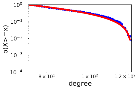
(a) input.

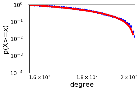
(b) fc1.

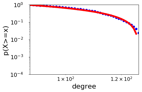
(c) fc2.

Figure 1: Log-log CCDF plot and TPL fit (red) for the MLP layers on MNIST. “fc1” and “fc2” denote the first and second FC layer, respectively. The softmax layer, which is not pruned, is not shown.

3.2 Convolutional Neural Network on MNIST

In this section, we use the convolutional neural network (CNN) in the Lasagne package. It is similar to LeNet-5 [19], and has two convolutional layers followed by 2 fully connected layers:

$$\text{\em input}-32C5-\text{\em MP}2-32C5-\text{\em MP}2-256\text{\em FC}-10\text{\em softmax}$$

Here, $32C5$ denotes a ReLU convolution layer with $32$ $5\times 5$ filters, and $\text{\em MP}2$ is a $2\times 2$ max-pooling layer. We use SGD with momentum as the optimizer. The other hyperparameters are the same as in the Lasagne package. The maximum number of epochs is $200$. The (dense) CNN has a testing accuracy of 98.85%. This is then pruned using the method in [12], with $s=0.7$. After retraining, the sparse CNN has a testing accuracy of 98.78%, and is comparable with the dense network.

For a convolutional layer, we consider each feature map at the convolutional layer as a node. As in Section 3.1, the node degree is obtained by counting the total number of connections (after pruning) to its upper and lower layers. As an example, consider a feature map (node) in the first convolutional layer (conv1). As the input image is of size $28\times 28$, each such feature map is of size $24\times 24$. To illustrate the counting more easily, we consider the unpruned network. We first count its connections to the input layer. Recall that in conv1, (i) the filter size is $5\times 5$; (ii) each filter weight is used $24\times 24=576$ times; and (iii) there is only one channel in the grayscale MNIST image. Thus, each node has $25\times 576\times 1=14,400$ connections to the input layer. Similarly, for connections to the conv2 layer, (i) the conv2 filter size is $5\times 5$; (ii) each filter weight is used $8\times 8=64$ times (size of each conv2 feature map); and (iii) there are 32 feature maps in conv2. Thus, each conv1 node has $25\times 64\times 32=51,200$ connections to the conv2 layer. Hence, the degree of each conv1 node (in an unpruned network) is $14,400+51,200=65,600$. Note that the pooling layers do not have learnable connections. They are never sparsified, and we do not need to study their degree distributions.

Figure 2 shows the CCDF plot and TPL fit for each CNN layer. Again, the TPL fits the distributions well.

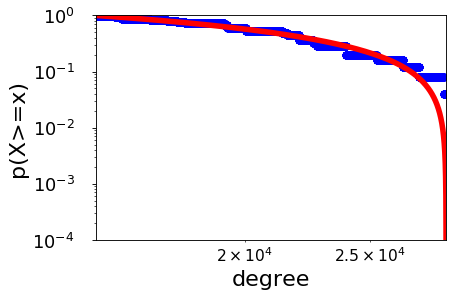
(a) conv1.

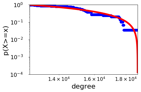
(b) conv2.

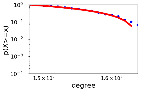
(c) fc3.

Figure 2: Log-log CCDF plot and TPL fit (red) for the CNN layers on MNIST. Here, “conv1” and “conv2” denote the first and second convolutional layers, and “fc3” is the 3rd (FC) layer.

3.3 CNN on CIFAR-10

In this section, we perform experiments on the CIFAR-10 data set, which contains $32\times 32$ color images from ten object classes. We use $45,000$ images for training, another $5,000$ for validation, and the remaining $10,000$ for testing. The following CNN from [20] is used:

$$\text{\em input}-32C3-32C3-\text{\em MP}2-64C3-64C3-\text{\em MP}2$$

$$-512\text{\em FC}-10\text{\em softmax}.$$

We use RMSprop as the optimizer, and the maximum number of epochs is $100$. The (dense) CNN has a testing accuracy of 81.90%. This is then pruned using the method in [12], with $s=0.7$. After retraining, the testing accuracy of the sparse CNN is 80.46%, and is comparable with the original network. Figure 3 shows the CCDF plot and TPL fit for each layer. Again, the TPL fits the distributions well.

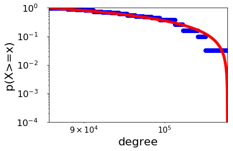
(a) conv1.

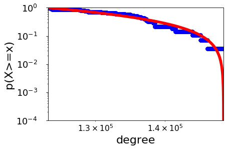
(b) conv2.

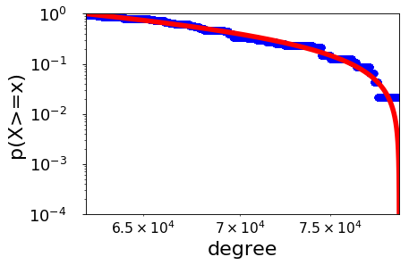
(c) conv3.

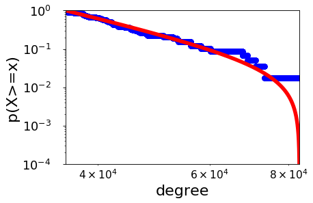
(d) conv4.

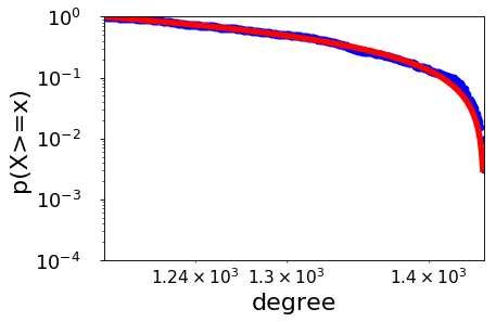
(e) fc5.

Figure 3: Log-log CCDF plot and TPL fit (red) for the CNN layers on CIFAR-10.

3.4 AlexNet on ImageNet

In this section, we perform experiments on the ImageNet data set [21], which has 1,000 categories, over 1.2 million training images, 50,000 validation images, and 100,000 test images. We use the sparsified AlexNet (with 5 convolutional layers and 3 fully connected layers) from [10]. Figure 4 shows the CCDF plot and TPL fit for the various AlexNet layers.

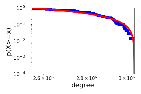
(a) conv1.

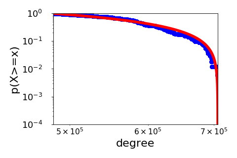
(b) conv2.

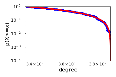
(c) conv3.

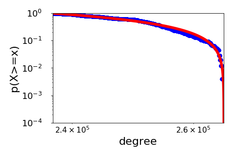
(d) conv4.

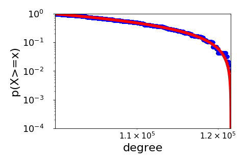
(e) conv5.

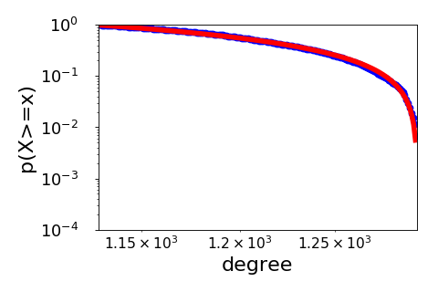
(f) fc6.

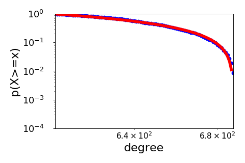
(g) fc7.

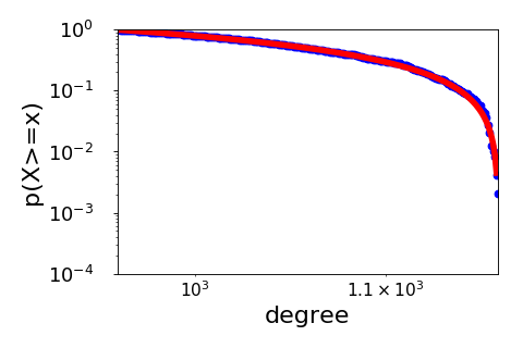
(h) fc8.

Figure 4: Log-log CCDF plot and TPL fit (red) for the sparse AlexNet layers. Naming of the layers follows that defined in Caffe.

3.5 VGG-16 on ImageNet

In this section, we use the (dense) VGG-16 model (with 13 convolutional layers and 3 fully connected layers) obtained by the dense-sparse-dense (DSD) procedure of [22]. We then prune this using the method in [22] with $s=0.3$. The top-1 and top-5 testing accuracies for the original dense CNN are 68.50% and 88.68%, respectively, while those of the sparse CNN are 71.81% and 90.77%. Figure 5 shows the CCDF plot and TPL fit for various layers.

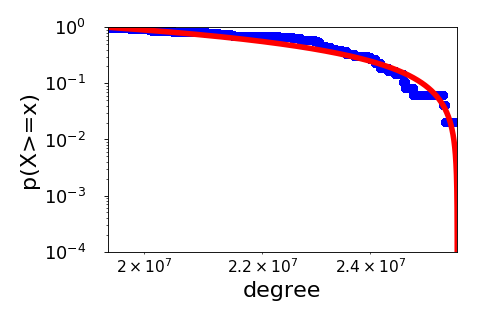
(a) conv1_1.

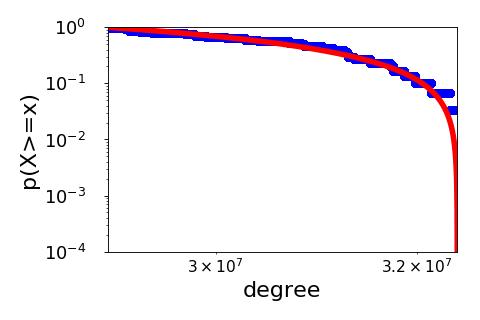
(b) conv1_2.

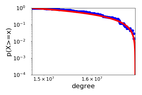
(c) conv2_1.

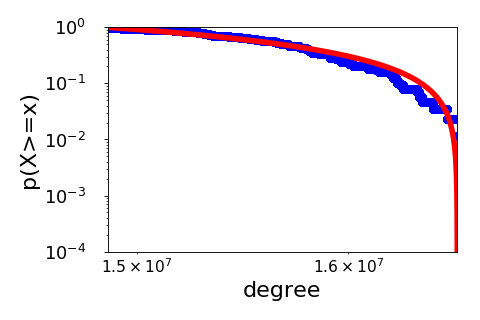
(d) conv2_2.

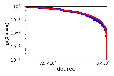
(e) conv3_1.

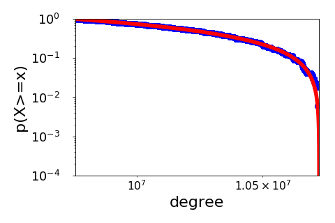
(f) conv3_2.

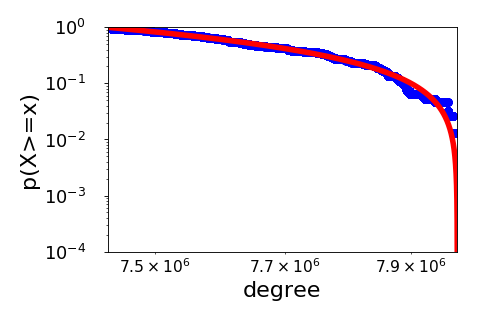
(g) conv3_3.

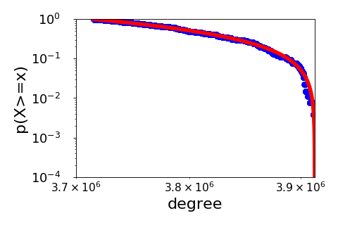
(h) conv4_1.

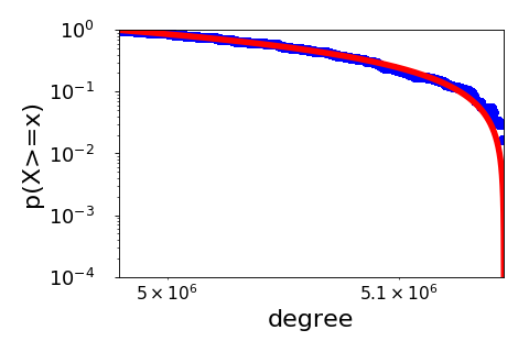
(i) conv4_2.

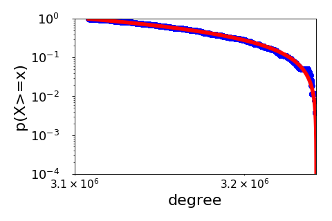
(j) conv4_3.

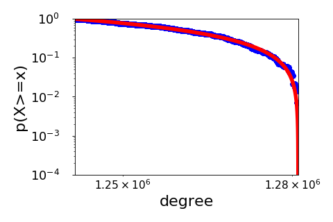
(k) conv5_1.

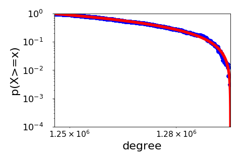
(l) conv5_2.

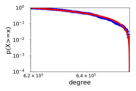
(m) conv5_3.

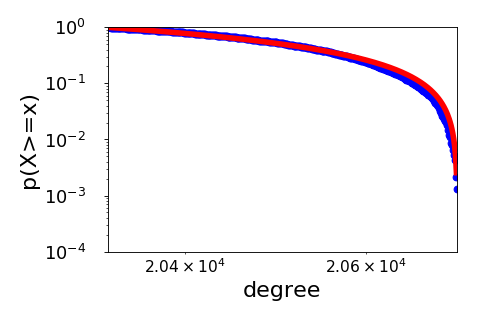
(n) fc6.

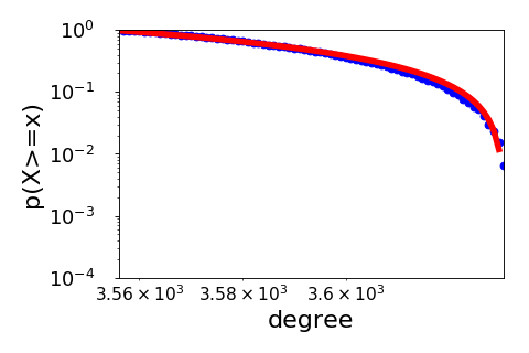
(o) fc7.

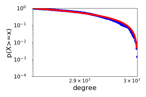
(p) fc8.

Figure 5: Log-log CCDF plot and TPL fit (red) for the VGG-16 layers. Naming of the layers follows that defined in Caffe.

4 Internal Preferential Attachment in NN

To study the dynamical properties of neural network connectivity, we consider the continual learning setting in which consecutive tasks are learned [13]. Specifically, at time $t=0$, an initial sparse network is trained to learn the first task. At each following timestep $t=1,2,\dots$, a new task is encountered, and the network is re-trained on the new task. We assume that only new connections, but not new nodes, can be added. Hence, preferential attachment, if exists, can only be internal but not external.

4.1 Evolution of the Degree Distribution

In this section, we assume that only nodes in adjacent layers can be connected, as is common in feedforward neural networks. Consider a pair of nodes, one from layer $l$ with degree $d_{1}$ and the other from layer $(l+1)$ with degree $d_{2}$. If internal preferential attachment exists, the number of connections between this node pair grows proportional to the product $d_{1}d_{2}$. Analogous to (5), the number of connections created per unit time between this node pair at time $t$ is:

$$\Delta_{t}^{l}(d_{1},d_{2})=N^{l}a^{l}\frac{d_{1}d_{2}}{\sum_{s,m}d_{s}d_{m}},$$ (6)

where $s$ and $m$ are indices to all the nodes in the two layers involved, $N^{l}$ is the number of nodes in layer $l$, and $a^{l}$ is the number of new internal connections created in unit time from a node in layer $l$ to layer $(l+1)$.

Next, we study how the degree of a node evolves. For node $i$ at layer $l$, let $d_{i}(t)$ be its degree at time $t$. Out of these $d_{i}(t)$ connections, let $d_{i}^{\uparrow}(t)$ be connected to the upper layer, and $d_{i}^{\downarrow}(t)$ to the lower layer. Using (6), the increase of its degree due to new connections to the upper layer is:

$$\frac{\mathrm{d}d_{i}^{\uparrow}(t)}{\mathrm{d}t} = \sum_{m}\Delta^{l}_{t}(d_{i}(t),d_{m}(t))$$

$$= N^{l}a^{l}d_{i}(t)\frac{\sum_{m}d_{m}(t)}{(\sum_{s}d_{s}(t))(\sum_{m}d_{m}(t))}$$

$$= \frac{N^{l}a^{l}d_{i}(t)}{\sum_{s}d_{s}(t)},$$

where $m$ and $s$ are indices to all the nodes in layer $(l+1)$ and layer $l$, respectively. Similarly, the increase of degree due to new connections to the lower layer is:

$$\frac{\mathrm{d}d_{i}^{\downarrow}(t)}{\mathrm{d}t}=\sum_{r}\Delta^{l-1}_{t}(d_{r}(t),d_{i}(t))=\frac{N^{l-1}a^{l-1}d_{i}(t)}{\sum_{s}d_{s}(t)},$$

where $r$ and $s$ are indices to all the nodes in layer $(l-1)$ and layer $l$, respectively. The total number of new connections for nodes in layer $l$ can be obtained as:

$$\sum_{s}d_{s}(t) = \sum_{s}d_{s}(0)+\int_{0}^{t}(N^{l}a^{l}+N^{l-1}a^{l-1})dt$$

$$= \sum_{s}d_{s}(0)+(N^{l}a^{l}+N^{l-1}a^{l-1})t.$$

Combining all these, we have

$$\frac{\mathrm{d}d_{i}(t)}{\mathrm{d}t} = \frac{\mathrm{d}d_{i}^{\uparrow}(t)}{\mathrm{d}t}+\frac{\mathrm{d}d_{i}^{\downarrow}(t)}{\mathrm{d}t}$$ (7)

$$= \frac{(N^{l}a^{l}+N^{l-1}a^{l-1})d_{i}(t)}{\sum_{s}d_{s}(0)+(N^{l}a^{l}+N^{l-1}a^{l-1})t}.$$

After integration and simplification, we obtain

$$d_{i}(t)=d_{i}(0)c^{l}(t),$$ (8)

where $c^{l}(t)=1+\frac{(N^{l}a^{l}+N^{l-1}a^{l-1})t}{\sum_{s}d_{s}^{l}(0)}$. Hence, $d_{i}(t)$ is linear w.r.t. the node’s initial degree $d_{i}(0)$. In particular, assume that the degree distribution of layer $l$ at $t=0$ (denoted $p_{0}^{l}$) follows the power law (standard or TPL), i.e., $p_{0}^{l}(d)=Ad^{-\alpha}$ for some $A>0$ and $\alpha>1$. Then, from (8), its degree distribution at time $t$ is:

$$p_{t}^{l}(d)=p_{0}^{l}\left(\frac{d}{c^{l}(t)}\right)=A\left(\frac{d}{c^{l}(t)}\right)^{-\alpha}\!\!\!\!\!\!=\!(c^{l}(t))^{\alpha}Ad^{-\alpha},$$ (9)

which follows the same power law as $p_{0}^{l}$, but scaled by the factor $(c^{l}(t))^{\alpha}$.

Remark 4.1

Note from (8) that as $c^{l}(t)$ increases with $t$, hence $d_{i}(t)$ increases with $t$. However, as we assume that new nodes cannot be added, the degree cannot grow infinitely and (8) will not hold for large $t$.

4.2 Experiments

We consider a simple continual learning setting with only two tasks. Experiments are performed on the MNIST data set, with the same setup in Section 3.1. The two tasks are from [23, 13]. Task A uses the original images, while task B uses images in which pixels inside a central $P\times P$ square are permuted. As in [13]), we use $P=8$ and 26. Note that as the size of MNIST image is $28\times 28$, when $P=26$, the task B (permuted) images are very different from the task A (original) images.

We first train a dense network on task A (Figure 6). A fraction of $s_{1}=0.9$ connections are pruned from each layer as in Section 3. The remaining connections are retrained on task A, and then frozen. Next, we reinitialize the pruned connections and train a dense network on task B. Another fraction of $s_{2}=0.8$ connections from each layer are again pruned and the remaining connections retrained. Recall that connections learned on task A are frozen, and so they will not be pruned or retrained. Table I shows the testing accuracies of the four networks in Figure 6. As can be seen, the sparse network has good performance on both tasks.

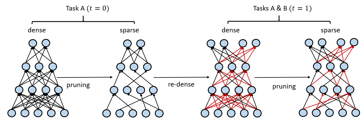
Figure 6: The continual learning setup. Connections learned for task A are in black, and those for task B are in red. Left: A dense network is trained on task A; Middle left: Network pruned and retrained on task A; Middle right: The pruned connections are reinitialized and retrained on task B; Right: Connections are pruned and the remaining connections retrained on task B.

TABLE I: Testing accuracies (%) for networks in the continual learning experiment.

	task A		task B
$P$	dense	sparse	dense	sparse
8	98.09	98.21	98.17	98.09
26	98.09	98.21	98.04	98.16

4.2.1 Existence of Internal Preferential Attachment

Empirically, $\Delta_{t}^{l}(d_{1},d_{2})$ in (6) can be estimated by counting the number of new connections created at time $(t+1)$ between all the involved node pairs (i.e., one from layer $l$ with degree $d_{1}$ and the other from layer $(l+1)$ with degree $d_{2}$ at time $t$), and then divide it by the number of such node pairs. Figure 7 shows this empirical estimate at time $t=0$ (denoted $\hat{\Delta}_{0}^{l}(d_{1},d_{2})$) versus the degrees $d_{1}$ and $d_{2}$. As can be seen, $\hat{\Delta}_{0}^{l}(d_{1}d_{2})$ increases with $d_{1}$ and $d_{2}$, indicating the presence of internal preferential attachment.

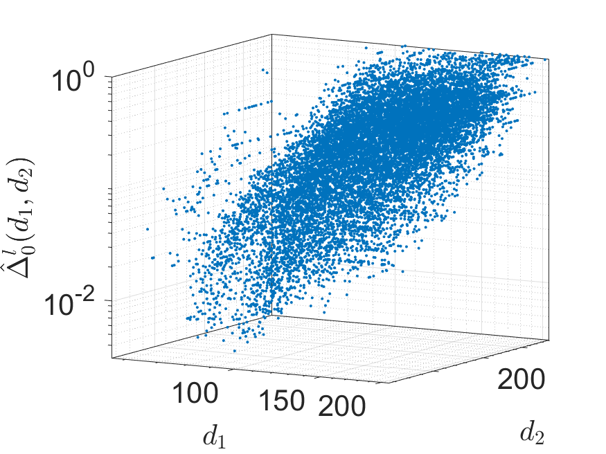
(a) input-to-fc1.

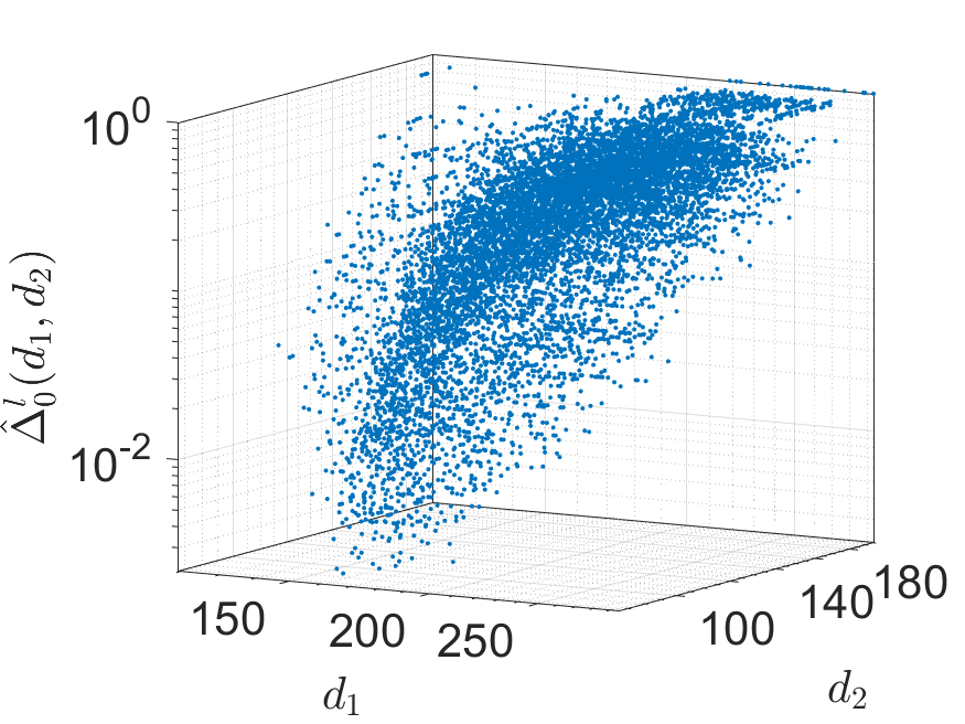
(b) fc1-to-fc2.

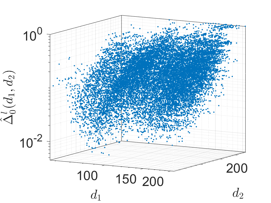
(c) input-to-fc1.

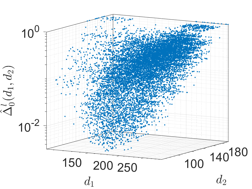
(d) fc1-to-fc2.

Figure 7: $\hat{\Delta}_{0}^{l}(d_{1},d_{2})$ vs $d_{1}$ and $d_{2}$. Top: $P=8$; Bottom: $P=26$.

4.2.2 Number of New Connections versus Degree

From (7), for a node with degree $d_{i}(0)$ at $t=0$, the number of connections added to it at $t=1$ is equal to

$$\left.\frac{\mathrm{d}d_{i}(t)}{\mathrm{d}t}\right|_{t=0}=d_{i}(0)\frac{N^{l}a^{l}+N^{l-1}a^{l-1}}{\sum_{s}d_{s}(0)}.$$ (10)

Let $d_{i}(0)=d$, an empirical estimate of $\left.\frac{\mathrm{d}d_{i}(t)}{\mathrm{d}t}\right|_{t=0}$ (denoted $\hat{\Omega}_{0}^{l}(d)$) can be obtained by counting the number of new connections that all nodes (from layer $l$) with degree $d$ made at time $(t+1)$, and then divide it by the number of degree-$d$ nodes (in layer $l$) at time $t$.

Figure 8 shows $\hat{\Omega}_{0}^{l}(d)$ versus the node degree $d$ at time $t=0$. As can be seen, when the two tasks are similar ($P=8$), the relationship is roughly linear for all layers, which agrees with (10). However, when the tasks are much less similar ($P=26$), the network must learn to associate new collections from pixels to penstrokes, and connections from the input layer to the first hidden layer have to be significantly modified. Hence, preferential attachment is no longer useful. As can be seen, there is no linear relationship for the input layer, and the linear relationship in the fc1 layer is noisier than that for $P=8$. On the other hand, as discussed in [23], once the input layer has established new associations to map from pixels to penstrokes, the higher-level feature extractors (i.e., fc2) are only dependent on these penstroke features (extracted at fc1) and thus less affected by the input permutation. As can be seen, the fc2 layer still shows a linear relationship.

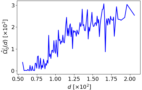
(a) input.

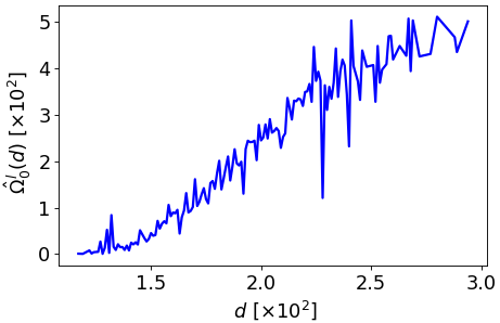
(b) fc1.

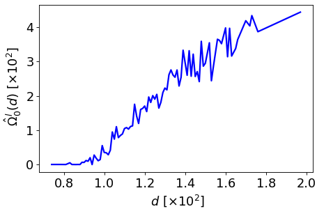
(c) fc2.

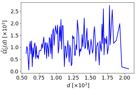
(d) input.

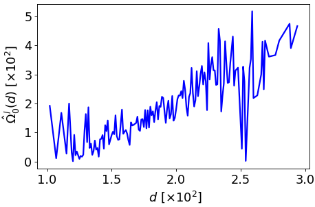
(e) fc1.

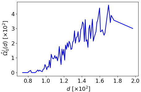
(f) fc2.

Figure 8: Number of new connections $\hat{\Omega}_{0}^{l}(d)$ vs degree $d$. Top: $P=8$; Bottom: $P=26$.

4.2.3 Degree Distribution

Recall from Section 3.1 that the degree distribution of the sparse MLP trained on task A ($t=0$) follows the TPL. From (9), we thus expect that its degree distribution after training on task B ($t=1$) also follows the TPL. Figure 9 shows the CCDF plot and TPL fit for each layer of the sparse network at $t=1$. As can be seen, the $p$-values of the first layer are relatively low. This is because that, due to permutation, the input layer has to establish new associations to map from pixels to penstrokes.

(a) input.

(b) fc1.

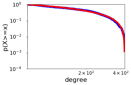
(c) fc2.

(d) input.

(e) fc1.

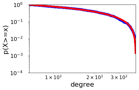
(f) fc2.

Figure 9: Log-log CCDF plot and TPL fit (red) for the MLP layers on MNIST at $t=1$. Top: $P=8$; Bottom: $P=26$.

5 Conclusion

In this paper, we showed that a number of sparse deep learning models exhibit the (truncated) power law behavior. We also proposed an internal preferential attachment model to explain how the network topology evolves, and verify in a continual learning setting that new connections added to the network indeed have this preferential bias.

In biological neural networks with limited capacities, reuse of neural circuits is essential for learning multiple tasks, and scale-free networks can learn faster than random and small-world networks [2]. In the future, we will use the dynamic behavior observed on artificial neural networks to design faster continual learning algorithms. Moreover, this paper only studies feedforward neural networks. We will also study existence of the power law in recurrent neural networks.

References

- [1] A. L. Barabási and R. Albert, “Emergence of scaling in random networks,” Science, vol. 286, no. 5439, pp. 509–512, 1999.
- [2] R. L. S. Monteiro, T. K. G. Carneiro, J. R. A. Fontoura, V. L. da Silva, M. A. Moret, and H. B. de Barros Pereira, “A model for improving the learning curves of artificial neural networks,” PloS One, vol. 11, no. 2, p. e0149874, 2016.
- [3] V. M. Eguiluz, D. R. Chialvo, G. A. Cecchi, M. Baliki, and A. V. Apkarian, “Scale-free brain functional networks,” Physical Review Letters, vol. 94, no. 1, p. 018102, 2005.
- [4] A. Clauset, C. R. Shalizi, and M. E. J. Newman, “Power-law distributions in empirical data,” SIAM Review, vol. 51, no. 4, pp. 661–703, 2009.
- [5] S. M. Burroughs and S. F. Tebbens, “Upper-truncated power laws in natural systems,” Pure and Applied Geophysics, vol. 158, no. 4, pp. 741–757, 2001.
- [6] L. A. N. Amaral, A. Scala, M. Barthelemy, and H. E. Stanley, “Classes of small-world networks,” Proceedings of the National Academy of Sciences, vol. 97, no. 21, pp. 11 149–11 152, 2000.
- [7] Y. Iturria-Medina, R. C. Sotero, E. J. Canales-Rodríguez, Y. Alemán-Gómez, and L. Melie-García, “Studying the human brain anatomical network via diffusion-weighted mri and graph theory,” Neuroimage, vol. 40, no. 3, pp. 1064–1076, 2008.
- [8] D. Kolyukhin and A. Torabi, “Power-law testing for fault attributes distributions,” Pure and Applied Geophysics, vol. 170, no. 12, pp. 2173–2183, 2013.
- [9] Y. LeCun, Y. Bengio, and G. Hinton, “Deep learning,” Nature, vol. 521, no. 7553, pp. 436–444, 2015.
- [10] S. Han, H. Mao, and W. J. Dally, “Deep compression: Compressing deep neural networks with pruning, trained quantization and huffman coding,” in International Conference of Learning Representations, 2016.
- [11] H. Li, A. Kadav, I. Durdanovic, H. Samet, and H. P. Graf, “Pruning filters for efficient convnets,” in International Conference of Learning Representations, 2017.
- [12] S. Han, J. Pool, J. Tran, and W. Dally, “Learning both weights and connections for efficient neural network,” in Advances in Neural Information Processing Systems, 2015, pp. 1135–1143.
- [13] J. Kirkpatrick, R. Pascanu, N. Rabinowitz, J. Veness, G. Desjardins, A. A. Rusu, K. Milan, J. Quan, T. Ramalho, A. Grabska-Barwinska et al., “Overcoming catastrophic forgetting in neural networks,” Proceedings of the National Academy of Sciences, vol. 114, no. 13, pp. 3521–3526, 2017.
- [14] M. L. Anderson, “Neural reuse: A fundamental organizational principle of the brain,” Behavioral and Brain Sciences, vol. 33, no. 4, pp. 245–266, 2010.
- [15] C. Fernando, D. Banarse, C. Blundell, Y. Zwols, D. Ha, A. A. Rusu, A. Pritzel, and D. Wierstra, “Pathnet: Evolution channels gradient descent in super neural networks,” Preprint arXiv:1701.08734, 2017.
- [16] A. Barabâsi, H. Jeong, Z. Néda, E. Ravasz, A. Schubert, and T. Vicsek, “Evolution of the social network of scientific collaborations,” Physica A: Statistical Mechanics and its Applications, vol. 311, no. 3, pp. 590–614, 2002.
- [17] B. D. Malamud, G. Morein, and D. L. Turcotte, “Forest fires: An example of self-organized critical behavior,” Science, vol. 281, no. 5384, pp. 1840–1842, 1998.
- [18] R. Hanel, B. Corominas-Murtra, B. Liu, and S. Thurner, “Fitting power-laws in empirical data with estimators that work for all exponents,” PloS one, vol. 12, no. 2, p. e0170920, 2017.
- [19] Y. LeCun, L. Bottou, Y. Bengio, and P. Haffner, “Gradient-based learning applied to document recognition,” Proceedings of the IEEE, vol. 86, no. 11, pp. 2278–2324, 1998.
- [20] F. Zenke, B. Poole, and S. Ganguli, “Continual learning through synaptic intelligence,” in International Conference on Machine Learning, 2017, pp. 3987–3995.
- [21] O. Russakovsky, J. Deng, H. Su, J. Krause, S. Satheesh, S. Ma, Z. Huang, A. Karpathy, A. Khosla, M. Bernstein, A. Berg, and F.-F. Li, “ImageNet large scale visual recognition challenge,” International Journal of Computer Vision, vol. 115, no. 3, pp. 211–252, 2015.
- [22] S. Han, J. Pool, S. Narang, H. Mao, S. Tang, E. Elsen, B. Catanzaro, J. Tran, and W. J. Dally, “DSD: Regularizing deep neural networks with dense-sparse-dense training flow,” in International Conference of Learning Representations, 2017.
- [23] I. J. Goodfellow, M. Mirza, D. Xiao, A. Courville, and Y. Bengio, “An empirical investigation of catastrophic forgetting in gradient-based neural networks,” Preprint arXiv:1312.6211, 2013.