Scheduling Wireless Links in the Physical Interference Model by Fractional Edge Coloring

Abstract

We consider the problem of scheduling the links of wireless mesh networks for capacity maximization in the physical interference model. We represent such a network by an undirected graph $G$, with vertices standing for network nodes and edges for links. We define network capacity to be $1/\chi^{\prime*}_{\mathrm{phys}}(G)$, where $\chi^{\prime*}_{\mathrm{phys}}(G)$ is a novel edge-chromatic indicator of $G$, one that modifies the notion of $G$’s fractional chromatic index. This index asks that the edges of $G$ be covered by matchings in a certain optimal way. The new indicator does the same, but requires additionally that the matchings used be all feasible in the sense of the physical interference model. Sometimes the resulting optimal covering of $G$’s edge set by feasible matchings is simply a partition of the edge set. In such cases, the index $\chi^{\prime*}_{\mathrm{phys}}(G)$ becomes the particular case that we denote by $\chi^{\prime}_{\mathrm{phys}}(G)$, a similar modification of $G$’s well-known chromatic index. We formulate the exact computation of $\chi^{\prime*}_{\mathrm{phys}}(G)$ as a linear programming problem, which we solve for an extensive collection of random geometric graphs used to instantiate networks in the physical interference model. We have found that, depending on node density (number of nodes per unit deployment area), often $G$ is such that $\chi^{\prime*}_{\mathrm{phys}}(G)<\chi^{\prime}_{\mathrm{phys}}(G)$. This bespeaks the possibility of increased network capacity by virtue of simply defining it so that edges are colored in the fractional, rather than the integer, sense.

Keywords: Wireless mesh networks, Link scheduling, Physical interference model, Edge coloring, Fractional edge coloring.

1 Introduction

We consider a set of nodes operating under the constraints imposed by the physical interference model of wireless communication [1]. These nodes are interconnected by a set $L$ of links, each link $e\in L$ being characterized by a sender node $s_{e}$ and a receiver node $r_{e}$. Any node may in principle act either as sender or as receiver, depending on the links in which it participates. When all links in a set $S\subseteq L$ are concomitantly active, the ability of receiver $r_{e}$ to decode what it receives from sender $s_{e}$ for any given link $e\in S$ is constrained by the signal-to-interference-plus-noise ratio (SINR) that results from the combined activity of the group, given by

$$\mathrm{SINR}(e,S)=\frac{P/d_{s_{e}r_{e}}^{\alpha}}{\gamma+\sum_{f\in S\setminus\{e\}}P/d_{s_{f}r_{e}}^{\alpha}}.$$ (1)

In this expression, $P$ is a node’s transmission power (assumed the same for all nodes), $\gamma$ is the noise floor, $d_{ab}$ is the Euclidean distance between nodes $a$ and $b$, and $\alpha>2$ is used to determine how power decays away from the transmitter with the distance to it.

The way the SINR constraint operates is by affecting the so-called feasibility of set $S$. Specifically, we say that a nonempty $S\subseteq L$ is feasible if no two of its links share a node and, additionally, $\mathrm{SINR}(e,S)\geq\beta$ for all $e\in S$, where $\beta>1$ is a parameter related to a receiver’s decoding capabilities, assumed the same for all receivers. For consistency, we assume that the link set $L$ is such that, for any singleton $\{e\}\subseteq L$, it holds that $P/\gamma d_{s_{e}r_{e}}^{\alpha}\geq\beta$. That is, every link in $L$ is capable of providing effective communication from its sender to its receiver when operating in isolation. Equivalently, set $\{e\}$ is assumed feasible.

The problem of maximizing network capacity, broadly understood as the rate of effective communication among nodes, is closely related to that of scheduling the links in $L$ for operation. This, in turn, is often posed under the so-called physical interference model (in which the SINR constraint is fully taken into account) but sometimes assumes only the constraints imposed by the so-called protocol-based interference model (which depend essentially on graph-based distances). Solving the link-scheduling problem may require computationally hard combinatorial problems to be tackled and has given rise to numerous proposals, some approaching the scheduling problem by itself [2, 3, 4, 5, 6, 7, 8, 9, 10, 11, 12, 13, 14, 15, 16, 17, 18, 19, 20, 21], some in conjunction with others [22, 23, 24, 25, 26, 27, 28, 29, 30, 31].

Many of these proposals are formulated within the framework of spatial time-division multiple access (STDMA), which divides time into slots and reduces the scheduling problem to the selection of which links to activate simultaneously in each one. The type of selection strategy that is by far the most adopted asks that a sequence $\mathcal{S}=\langle S_{1},S_{2},\ldots,S_{T}\rangle$ be determined for some $T>1$. In this sequence, each $S_{i}$ is a subset of the link set $L$ complying with the constraints imposed by the interference model in use and moreover ensuring that each $e\in L$ appears in exactly one of the $T$ subsets. Any approach to maximize network capacity by solving the link-scheduling problem will therefore seek to minimize $T$ (maximize $1/T$) without violating any of these constraints. Once a solution is available, repeating the sequence $\mathcal{S}$ guarantees interference-free communication for as long as needed.

One common abstraction for reasoning about such proposals is that of graph coloring or related notions. Of the proposals mentioned above, some do indeed make explicit reference to such an abstraction [22, 2, 8, 11, 31, 18, 21]. In terms of the formulation outlined above, clearly the links in each set $S_{i}$, to be scheduled for operation in the same time slot, can be regarded as being assigned the same color (the $i$th of the $T$ available colors) if we interpret the conditions for membership in $S_{i}$ in the context of graph coloring. Whether it is vertex coloring or edge coloring that is being considered depends on how the graph in question is set up to represent how the various links relate to each other given the interference model at hand. In either case, once the least possible value of $T$ is found (or approximated), each vertex or edge ends up having exactly one color.

To the best of our knowledge, the decades-long effort to come up with capacity-optimizing strategies for link scheduling has almost completely failed to recognize that such a single-color abstraction is inherently limited and may in many cases fall short of leading to as much network capacity as possible. The exceptions we know of are only three and separated by many years. The earliest one is based on the coloring of a graph’s edges and adopts what would pass for the protocol-based interference model had it existed at the time [22]. The other two are very recent and both based on the coloring of vertices, the earliest one given for the protocol-based interference model as well [31], the latest for the physical interference model [21].

What these three proposals have in common is that they use the fractional variety of graph coloring. In terms of the STDMA scheme explained above, what they do is let each link appear in exactly $q\geq 1$ of the $T$ sets in $\mathcal{S}$, the same value of $q$ for all links, instead of in one single set. Moreover, instead of minimizing $T$ alone, they seek to minimize the ratio $T/q$ while treating $q$ as a variable. If $T^{1}$ is the least number of slots to accommodate all $|L|$ link activations, one per link, in the single-color case, and if the pair $(T^{*},q^{*})$ provides the least possible $T/q$ ratio while accommodating all $q|L|$ link activations, $q$ per link, in the fractional-coloring case, then conceivably it may happen that $T^{*}/q^{*}<T^{1}$. If this does happen, then clearly we have $T^{*}<T^{1}q^{*}$, so the $T^{*}$-slot sequence is shorter than $q^{*}$ repetitions of the $T^{1}$-slot sequence and therefore the former is preferable to the latter, since in the two cases we have the same total number of link activations, viz., $q^{*}|L|$. Readily, in this case the sequence to be repeated in order for interference-free communication to be provided while needed is the one comprising $T^{*}$ sets. Thus, so far as we seek to maximize network capacity via link scheduling, what needs to be done is maximize the ratio $q/T$. This ratio is how we define network capacity henceforth.

Important though the fractional-coloring-based contributions in [22, 31, 21] have been, they have each left relevant problems open as well. As we see these problems, the most relevant one is the search for approaches for the exact determination of optimal fractional colorings in the physical interference model. As we remarked above, this has been attempted neither by the proposals in [22, 31] (both of which target the protocol-based interference model, though the former is exact while the latter is a heuristic) nor by the one in [21] (which is a heuristic, even if one for the physical interference model).

Our aim in this paper is to make some headway toward achieving such an exact method. As will become clear along the way, the difficulty lies not so much in the possibility of obtaining such an exact method of solution, which we do describe in detail, but rather in making its computational hardness scale in such a way that tackling large instances is still possible. The exact method we describe has allowed us to chart the landscape of a class of random networks regarding the possibility of fractional-coloring-based link scheduling that is superior to its single-color counterpart. We have been able to do this for a reasonably wide range of the parameters involved in network generation, which has led us to conclude that, given the uncertainties afforded by the confidence intervals obtained, networks with the potential to benefit from a fractional-coloring approach occur in a non-negligible proportion. These empirical findings, along with the implicit impetus they lend to the search for approaches that are more computationally efficient, constitute one of our contributions. (We also pinpoint possible alternatives that might lead to more scalable approaches, but finding them remains an open issue.) Our main contribution, though, is that by formulating capacity optimization in the framework of fractional coloring, we automatically provide for the fallback solution in which it is integer (single-color) coloring, rather than nontrivial fractional (more-than-one-color) coloring, that yields optimal capacity. Integer coloring, after all, is simply the particular case of fractional coloring in which it is better to use one, rather than more than one, color per link.

Before we proceed, a few remarks are in order about the particular view of network-capacity maximization we have adopted, that is, maximization via link scheduling in the physical interference model. While this view is the same as in [1, 3, 9, 17, 21], there are nevertheless various other issues that are sometimes taken into account. These include node placement [32, 33, 34, 35], frequency assignment [36, 37], as well as taking end-to-end communication demands into consideration [32, 36, 33, 34, 35] or not [37]. Moreover, even though some approaches do resort to vertex coloring that assigns more than one color to the same vertex [36, 3], they have remained oblivious to the fact that the real power of coloring the same vertex or edge by multiple colors lies in the potential to exploit the graph’s fractional-coloring properties (i.e., through the minimization of a rational, not an integer, number), not in color multiplicity per se.

We continue in the following manner. First, in Section 2, we give a detailed mathematical formulation of the fractional-coloring-based approach to link scheduling that we pursue. Then we move to Section 3, where our computational methodology is laid out. Our results are presented in Section 4, with discussion, and we finalize in Section 5 with a summary, concluding remarks, and comments on future prospects.

2 Mathematical formulation

Given the set $L$ of links to be scheduled, and letting $N$ be the set of all nodes acting as sender or receiver in at least one link in $L$, we consider the undirected graph $G=(N,L)$, that is, the graph having $N$ for set of vertices and $L$ for set of undirected edges. Our use of a graph and not a multigraph (which would allow multiple edges joining the same two vertices) is meant to allow us to use the same experimental setting as in [21]. As we discuss in Section 3, in that setting no two links are allowed to interconnect the same two nodes, not even in different directions (i.e., with their roles as sender or receiver reversed). We do make this assumption about $L$ henceforth, but the reader is to note that no further modeling difficulties would arise otherwise (cf. Section 5.1).

We begin with the presentation of a linear programming (LP) problem for the determination of maximum network capacity as defined in Section 1. That is, we aim to formulate the problem of finding the integers $T$ and $q$ that minimize the ratio $T/q$ while allowing every link in $L$ to be active in exactly $q$ of $T$ time slots while respecting the constraints imposed by the physical interference model.

2.1 LP problem

By the definition of a feasible set of links and also the definition of graph $G$ above, clearly every feasible set of links corresponds to a matching in $G$, though the converse may not be true. Henceforth we refer as a feasible matching to any matching whose edges constitute a feasible set of links.

Let $\mathcal{M}$ be the set of all feasible matchings of $G$. For each $M\in\mathcal{M}$, let $x_{M}$ be a real variable and consider the following LP problem.

minimize $$\textstyle w=\sum_{M\in\mathcal{M}}x_{M}$$ (2)

subject to $$x_{M}\geq 0, \forall M\in\mathcal{M}$$ (3)

$$\textstyle\sum_{M\in\mathcal{M}|e\in M}x_{M}=1. \forall e\in L$$ (4)

This problem asks that the sum of all $x_{M}$’s (the objective function $w$ in Eq. (2)) be minimized while respecting the constraints that none of them be allowed to become negative (Eq. (3)) and that, for each edge $e\in L$, those $x_{M}$’s for which $e\in M$ add up to $1$ (Eq. (4)). Because the coefficients of the $x_{M}$’s in Eqs. (2) and (4) are all equal to $1$, hence rational numbers, at least one solution exists minimizing $w$ with every $x_{M}$ a rational number as well. Let $\mathcal{P}$ be the subset of $\mathcal{M}$ such that $M\in\mathcal{P}$ if and only if $x_{M}>0$ in this solution.

For $M\in\mathcal{P}$, let $p_{M}/q_{M}$ be such positive rational value of $x_{M}$ minimizing $w$. If $q^{*}$ denotes the least common multiple of all $q_{M}$’s over $M\in\mathcal{P}$, then the desired minimum value of $w$, call it $w^{*}$, can be written as

$$w^{*}=\frac{\sum_{M\in\mathcal{P}}T_{M}}{q^{*}},$$ (5)

where $T_{M}=q^{*}p_{M}/q_{M}$ is necessarily a positive integer.

Now consider any edge $e\in L$ and let $\mathcal{P}_{e}$ be the subset of $\mathcal{P}$ such that $M\in\mathcal{P}_{e}$ if and only if $e\in M$. That is, $\mathcal{P}_{e}$ is the set of all feasible matchings $M$ of $G$ that contribute to the minimum value of $w$ with a positive $x_{M}$ and moreover include edge $e$. Set $\mathcal{P}_{e}$ is necessarily nonempty, since the matching containing $e$ and no other edge is by assumption feasible. By the constraint in Eq. (4), we have

$$\sum_{M\in\mathcal{P}_{e}}T_{M}=q^{*}\sum_{M\in\mathcal{P}_{e}}\frac{p_{M}}{q_{M}}=q^{*}.$$ (6)

If we view each $T_{M}\geq 1$ as a sort of multiplicity of matching $M$, then this equation is saying that the added multiplicities of all matchings in $\mathcal{P}_{e}$ equals $q^{*}$.

What this means in the context of scheduling the links in $L$ is that, if we let all links in $M$ be concomitantly active for $T_{M}$ time slots and do this for all $M\in\mathcal{P}_{e}$, then after all $\sum_{M\in\mathcal{P}_{e}}T_{M}$ time slots link $e$ will have appeared $q^{*}$ times, regardless of the particular link $e$ under consideration. Thus, ensuring that this happens for every $e\in L$ requires

$$\sum_{M\in\cup_{e\in L}\mathcal{P}_{e}}T_{M}=\sum_{M\in\mathcal{P}}T_{M}$$ (7)

time slots. We denote this overall number of time slots by $T^{*}$ and, by Eq. (5), conclude that $w^{*}=T^{*}/q^{*}$ is the desired minimum value of the ratio $T/q$.

2.2 Edge-coloring interpretation

If we allow $\mathcal{M}$ to include every one of the graph’s matchings, without regard to how any particular matching stands as far as our link-scheduling problem is concerned, then in graph-theoretic terms the preceding development explains why the LP problem given in Eqs. (2)–(4) can be taken as defining the fractional chromatic index of $G$ [38]. This index, which we denote by $\chi^{\prime*}(G)$, reflects the most “efficient” way in which the graph’s set of edges can be covered by $T$ matchings in such a way as to let each edge belong to exactly $q$ of the matchings. The use of efficient here refers to the minimization of the ratio $T/q$, hence the graph-theoretic interpretation in the case of an all-encompassing $\mathcal{M}$. The well-known, alternative definition of $\chi^{\prime*}(G)$ as

$$\chi^{\prime*}(G)=\min_{k\geq 1}\frac{\chi^{\prime k}(G)}{k}$$ (8)

is an easy consequence of the same development. In this expression, $\chi^{\prime k}(G)$ is the minimum number of matchings needed to cover $G$ in such a way that every edge belongs to exactly $k$ matchings. Setting $k=1$ yields the usual chromatic index of $G$, $\chi^{\prime}(G)=\chi^{\prime 1}(G)$, for which it then holds that

$$\chi^{\prime*}(G)\leq\chi^{\prime}(G).$$ (9)

By analogy, restricting $\mathcal{M}$ to include only feasible matchings admits a graph-theoretic interpretation as well. In this interpretation, the edge set $L$ of $G$ has to be covered by $T$ feasible matchings while mandatorily including every edge in exactly $q$ of them and minimizing $T/q$. A problem-specific fractional chromatic index can then be defined for $G$ based on Eqs. (2)–(4), one that takes into account all the specificities of the physical interference model discussed in Section 1 by requiring all members of $\mathcal{M}$ to be feasible. We denote this new index by $\chi^{\prime*}_{\mathrm{phys}}(G)$ and generalize Eqs. (8) and (9) in the obvious way, obtaining

$$\chi^{\prime*}_{\mathrm{phys}}(G)=\min_{k\geq 1}\frac{\chi^{\prime k}_{\mathrm{phys}}(G)}{k}$$ (10)

and

$$\chi^{\prime*}_{\mathrm{phys}}(G)\leq\chi^{\prime}_{\mathrm{phys}}(G),$$ (11)

where each $\chi^{\prime k}_{\mathrm{phys}}(G)$ is defined analogously to $\chi^{\prime k}(G)$ and $\chi^{\prime}_{\mathrm{phys}}(G)=\chi^{\prime 1}_{\mathrm{phys}}(G)$. In Section 5, we discuss how computationally hard it may be to determine $\chi^{\prime*}_{\mathrm{phys}}(G)$, especially vis-à-vis the determination of $\chi^{\prime*}(G)$. Be that as it may, clearly network capacity as defined in Section 1 is given by $1/\chi^{\prime*}_{\mathrm{phys}}(G)$.

2.3 Finding out whether $\chi^{\prime*}_{\mathrm{phys}}(G)<\chi^{\prime}_{\mathrm{phys}}(G)$

One of the core elements of our study in this paper is the determination, for some given $G$, of whether coloring its edges fractionally is more efficient (in the sense explained earlier) than coloring them with one single color per edge. Put differently, for each $G$ we must be able to determine whether the inequality in Eq. (11) is strict, which clearly is true if and only if the most efficient coloring of $G$’s edges employs $k>1$ colors per edge. Recall that solving the LP problem in Eqs. (2)–(4) already gives us the value of $\chi^{\prime*}_{\mathrm{phys}}(G)$ along with the corresponding $x_{M}$’s that are nonzero. It would then seem that checking whether all of these $x_{M}$’s equal $1$ suffices, since if they do we can immediately conclude that $\chi^{\prime*}_{\mathrm{phys}}(G)=\chi^{\prime}_{\mathrm{phys}}(G)$. However, that LP problem may admit several optimal solutions, including some that involve non-unit $x_{M}$’s even when another equally optimal solution involves unit $x_{M}$’s only. For this reason, testing whether every nonzero $x_{M}$ equals $1$ in the optimal solution returned by the LP solver is meaningful only in the affirmative case. In the negative case the test is meaningless, since it does not necessarily follow that $\chi^{\prime*}_{\mathrm{phys}}(G)<\chi^{\prime}_{\mathrm{phys}}(G)$ (cf. Section 3.1 for an example).

Given this difficulty, our approach is to address the direct calculation of $\chi^{\prime}_{\mathrm{phys}}(G)$ as well. We do this by modifying the LP program of Eqs. (2)–(4) so that each $x_{M}$ must be an integer equal to $0$ or $1$. The result is the following integer linear programming (ILP) problem.

minimize $$\textstyle w_{\mathrm{int}}=\sum_{M\in\mathcal{M}}x_{M}$$ (12)

subject to $$x_{M}\in\{0,1\}, \forall M\in\mathcal{M}$$ (13)

$$\textstyle\sum_{M\in\mathcal{M}|e\in M}x_{M}=1. \forall e\in L$$ (14)

Clearly, any valuation of the $x_{M}$’s satisfying the constraints in Eqs. (13) and (14) characterizes a partition of the link set $L$ into feasible matchings (specifically, a matching $M\in\mathcal{M}$ is in the partition if and only if $x_{M}=1$). The objective function in Eq. (12) counts the corresponding number of matchings and therefore its optimal value, call it $w^{*}_{\mathrm{int}}$, is such that $w^{*}_{\mathrm{int}}=\chi^{\prime}_{\mathrm{phys}}(G)$.

In summary, the following is how we find out out whether $\chi^{\prime*}_{\mathrm{phys}}(G)<\chi^{\prime}_{\mathrm{phys}}(G)$.

1. Find $\chi^{\prime*}_{\mathrm{phys}}(G)$ by solving the LP problem in Eqs. (2)–(4).

2. If every nonzero $x_{M}$ in the solution equals $1$, then conclude that $\chi^{\prime*}_{\mathrm{phys}}(G)=\chi^{\prime}_{\mathrm{phys}}(G)$ and stop.

3. Find $\chi^{\prime}_{\mathrm{phys}}(G)$ by solving the ILP problem in Eqs. (12)–(14).

4. Test whether $\chi^{\prime*}_{\mathrm{phys}}(G)<\chi^{\prime}_{\mathrm{phys}}(G)$.

Clearly, Steps 1–4 amount to solving the ILP problem only in those cases in which the solution to the LP problem is inconclusive as far as comparing $\chi^{\prime*}_{\mathrm{phys}}(G)$ and $\chi^{\prime}_{\mathrm{phys}}(G)$ is concerned.

3 Experimental setup

Given a fixed graph $G=(N,L)$, of vertex set $N$ and edge set $L$, the computational core of our experiments is carrying out Steps 1 and 3 of Section 2.3, which solve an LP problem and an ILP problem on $G$, respectively. In our experiments, graph $G$ is an instance of the following random geometric graph. Given a $d\times d$ region in two-dimensional Euclidean space, each of the $|N|$ vertices is placed in it uniformly at random. For vertices $a,b\in N$, the unordered pair $(a,b)$ is an edge of $L$ if and only if $d_{ab}\leq(P/\beta\gamma)^{1/\alpha}$ (equivalently, if and only if $\mathrm{SINR}((a,b),\{(a,b)\})\geq\beta$, where the role taken up by $a$ as sender or receiver relative to $b$ is immaterial). Put differently, $(a,b)$ is an edge in $G$ if and only if the singleton $\{(a,b)\}$ is feasible. For each $e=(a,b)\in L$, sender $s_{e}$ is either $a$ or $b$ uniformly at random, with receiver $r_{e}$ set correspondingly. This random graph is equivalent to what is called a type-I network in [21]. We use $\alpha=4$, $\beta=316.23$ ($25$ dB), and $\gamma=8\times 10^{-11}$ mW ($-100.97$ dBm), as well as $P=300$ mW ($24.78$ dBm) throughout all experiments.

For fixed $|N|$ and $d$, we generated $1\,000$ graph instances and tested each one for suitability to Steps 1–4. Failing instances were dropped, so all our results are expressed as averages over the passing instances. An instance can fail for at least one of three reasons: edge set $L$ is empty; edge set $L$ has more than $128$ edges, in which case we lack the computational resources to enumerate all feasible matchings that go in set $\mathcal{M}$; the number of feasible matchings in set $\mathcal{M}$ is greater than $50\times 10^{6}$, which is as far as we can go given $128$ GB of RAM and given that we use the Gurobi suite (www.gurobi.com) for solving both the LP and ILP problems, always with the pre-solver disabled and Simplex as the core linear programming solver (we found that these Gurobi settings require the least amount of RAM overall). The number of passing instances for each combination of $|N|$ and $d$ values we used is given in Table 1.

Table 1: Number of graph instances used for each $|N|,d$ combination.

	$d$ (km)
$|N|$	$1$	$2$	$3$	$4$	$5$	$6$	$7$	$8$	$9$	$10$
$10$	$1\,000$	$977$	$816$	$627$	$460$	$358$	$271$	$222$	$158$	$125$
$20$	$1\,000$	$1\,000$	$1\,000$	$985$	$929$	$830$	$720$	$618$	$524$	$450$
$30$	$178$	$1\,000$	$1\,000$	$1\,000$	$999$	$988$	$958$	$894$	$826$	$761$
$40$	$0$	$999$	$1\,000$	$1\,000$	$1\,000$	$1\,000$	$998$	$985$	$962$	$933$
$50$	$0$	$733$	$1\,000$	$1\,000$	$1\,000$	$1\,000$	$1\,000$	$999$	$994$	$983$
$60$	$0$	$1$	$1\,000$	$1\,000$	$1\,000$	$1\,000$	$1\,000$	$1\,000$	$998$	$996$
$70$	$0$	$0$	$879$	$999$	$1\,000$	$1\,000$	$1\,000$	$1\,000$	$1\,000$	$1\,000$
$80$	$0$	$0$	$0$	$927$	$993$	$1\,000$	$1\,000$	$1\,000$	$1\,000$	$1\,000$
$90$	$0$	$0$	$0$	$537$	$859$	$983$	$998$	$1\,000$	$1\,000$	$1\,000$
$100$	$0$	$0$	$0$	$72$	$405$	$818$	$946$	$988$	$998$	$1\,000$

In Table 1, a “main diagonal” is discernible whose entries all equal $1\,000$ and thus indicate combinations of $|N|$ and $d$ values for which none of the graph instances failed. Above this diagonal failures occur because $L$ turns out empty, which occurs more frequently as $|N|$ is decreased or $d$ is increased. Failures below the diagonal occur for at least one of the remaining two reasons, viz., an excessive number of edges in $L$ or an excessive number of feasible matchings in $\mathcal{M}$. Both forms of failure become more frequent with increasing $|N|$ or decreasing $d$, but failure by too many edges in $L$ is by far the most frequent of the two.

Given a $|N|,d$ pair, enumerating all the feasible matchings in $\mathcal{M}$ for a passing graph instance $G$ has taken on average up to about $597$ seconds to complete. Running Step 1 to find $\chi^{\prime*}_{\mathrm{phys}}(G)$, or Step 3 to find $\chi^{\prime}_{\mathrm{phys}}(G)$ whenever reaching that step, has required on average up to about $199$ and $3\,575$ seconds, respectively. These figures refer to an Intel Xeon E5-1650 v4 running at 3.6 GHz on 128 GB of RAM. Such maximum averages were all observed for $|N|=100$ and $d=4$ km. In view of these running times, it is unlikely that problem instances can be scaled up significantly while still being amenable to solution by exact methods. We return to this issue in Section 5.2.

3.1 Examples

Having described our methods to generate graph instance $G$ and to solve the corresponding LP and ILP problems, it is worth returning to the discussion of Section 2.3, with examples aiming to clarify the relationship between $\chi^{\prime*}_{\mathrm{phys}}(G)$ and $\chi^{\prime}_{\mathrm{phys}}(G)$ vis-à-vis the values of those problems’ variables at the optima they report. Two examples are given in Figure 1. They both contain non-unit variables in the solution to the LP problem, but $\chi^{\prime*}_{\mathrm{phys}}(G)$ relates differently to $\chi^{\prime}_{\mathrm{phys}}(G)$ in each case.

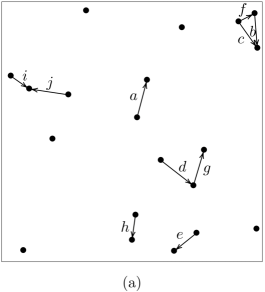
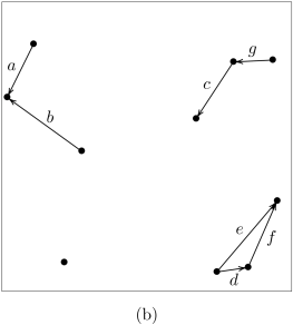
Figure 1: Sample graph instances $G$. The one in panel (a) was generated for $|N|=20$ and $d=2$ km, and turned out to have $|L|=10$ and $|\mathcal{M}|=29$. Its edge-chromatic properties were found to be such that $\chi^{\prime*}_{\mathrm{phys}}(G)=\chi^{\prime}_{\mathrm{phys}}(G)=6$. The graph instance in panel (b) was generated for $|N|=10$ and $d=1$ km, and has $|L|=7$ and $|\mathcal{M}|=10$. Its edge-chromatic properties are such that $\chi^{\prime*}_{\mathrm{phys}}(G)=11/2<6=\chi^{\prime}_{\mathrm{phys}}(G)$. Edges are drawn with directions to highlight their incident vertices’ roles as either sender nodes (the edges’ tail vertices) or receiver nodes (the edges’ head vertices).

The first example, given in panel (a) of the figure, refers to a graph instance $G$ for which $\chi^{\prime*}_{\mathrm{phys}}(G)=\chi^{\prime}_{\mathrm{phys}}(G)=6$. Detecting this, however, required solving both the LP problem (to discover the value of $\chi^{\prime*}_{\mathrm{phys}}(G)$) and the ILP problem (to discover the value of $\chi^{\prime}_{\mathrm{phys}}(G)$). Solving only the former problem and inspecting its variables’ values at the optimum revealed eight feasible matchings $M$ for which $x_{M}\neq 0$, four of them with $x_{M}=1$ (matchings $\{a\}$, $\{d\}$, $\{g\}$, and $\{b,j\}$), four others with $x_{M}=1/2$ (matchings $\{e,f\}$, $\{c,h\}$, $\{c,e,i\}$, and $\{f,h,i\}$). This illustrates why looking for non-unit variables at the optimum as a proxy for $\chi^{\prime*}_{\mathrm{phys}}(G)<\chi^{\prime}_{\mathrm{phys}}(G)$ can be misleading. In fact, in the case in question, solving the ILP problem brought up the possibility of ending up with six nonzero variables, all equal to $1$, corresponding to matchings $\{a\}$, $\{d\}$, $\{c,e\}$, $\{g\}$, $\{f,h,i\}$, and $\{b,j\}$. Had this been the solution returned to the LP problem to begin with, we would have known that $\chi^{\prime*}_{\mathrm{phys}}(G)=\chi^{\prime}_{\mathrm{phys}}(G)$ immediately and would have been able to dispense with the need to solve the ILP problem as well.

The example in panel (b), on the other hand, is such that $\chi^{\prime*}_{\mathrm{phys}}(G)=11/2<6=\chi^{\prime}_{\mathrm{phys}}(G)$, serving to illustrate those cases in which detecting non-unit variables at the optimum of the LP problem does indeed translate into a situation of $\chi^{\prime*}_{\mathrm{phys}}(G)<\chi^{\prime}_{\mathrm{phys}}(G)$ (even though, as in the previous example, this can only be known after the ILP problem is solved as well). In the case of Figure 1(b), the solution to the LP problem indicated seven feasible matchings $M$ for which $x_{M}\neq 0$, four with $x_{M}=1$ (matchings $\{b\}$, $\{c\}$, $\{e\}$, and $\{f\}$), three with $x_{M}=1/2$ (matchings $\{a,d\}$, $\{a,g\}$, $\{d,g\}$). As for the solution to the ILP problem, six nonzero variables were identified at the end, all equal to $1$, corresponding to matchings $\{b\}$, $\{c\}$, $\{d\}$, $\{e\}$, $\{f\}$, and $\{a,g\}$.

Further insight can be gained into the examples of Figure 1 by considering the actual schedules implied by the solutions to the LP and ILP problems. In either example, solving the corresponding LP problem yielded either $x_{M}=1$ or $x_{M}=1/2$ for all nonzero variables at the optimum. As discussed in Section 2.1, this implies that every matching $M$ for which $x_{M}=1$ is to appear in the resulting schedule with multiplicity $T_{M}=2$, while those with $x_{M}=1/2$ appear with multiplicity $T_{M}=1$. The number of slots in the schedule is the sum $T^{*}$ of all multiplicities. The number of times each edge appears in these $T^{*}$ slots, denoted by $q^{*}$, is the least common multiple of the denominators of all nonzero $x_{M}$’s at the optimum (in either example at hand, $q^{*}=2$). As for the solution to each ILP problem, the schedule it implies has a number $T^{1}$ of slots given by the sum of all $x_{M}$’s at the optimum. It is better to use multiple colors per edge whenever $T^{*}<T^{1}q^{*}$. This is not the case of the example in Figure 1(a), whose schedules are shown in Figures 2(a) and (b), but is the case of the example in Figure 1(b), whose schedules appear in Figures 2(c) and (d).

Figure 2: Schedules corresponding to the optimal solutions to the LP and ILP problems for the two examples of Figure 1. Panels (a) and (b) correspond to the example of Figure 1(a), the former panel depicting a single occurrence of the $T^{*}$-slot schedule implied by the solution to the LP problem, the latter depicting $q^{*}$ repetitions of the $T^{1}$-slot schedule implied by the solution to the ILP problem. We have $T^{*}=T^{1}q^{*}$, so the two are essentially equivalent. Panels (c) and (d) refer, correspondingly, to the example of Figure 1(b). Now we have $T^{*}<T^{1}q^{*}$, so the $T^{*}$-slot schedule is preferable.

4 Results and discussion

We give results in Figures 3, 4, and 5, with Figure 3 showing the percentage of those graph instances $G$ given in Table 1 for which $\chi^{\prime*}_{\mathrm{phys}}(G)<\chi^{\prime}_{\mathrm{phys}}(G)$. Such graph instances are cases of network-capacity improvement when substituting a schedule based on fractional edge coloring (of capacity $1/\chi^{\prime*}_{\mathrm{phys}}(G)$) for one based on edge coloring that employs one single color per edge (of capacity $1/\chi^{\prime}_{\mathrm{phys}}(G)$). The ratios of capacity improvement, given by $\chi^{\prime}_{\mathrm{phys}}(G)/\chi^{\prime*}_{\mathrm{phys}}(G)$, are shown in Figure 4 as averages over the pertinent graph instances $G$. The corresponding confidence intervals are given in Figure 5 as fractions of the corresponding means.

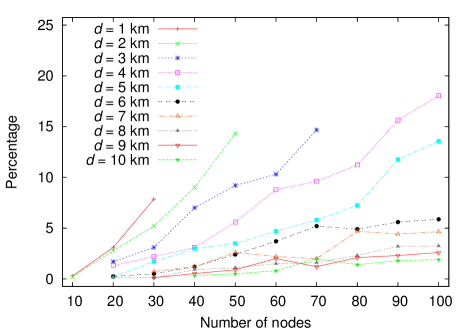
Figure 3: Percentage of the graph instances $G$ in Table 1 for which $\chi^{\prime*}_{\mathrm{phys}}(G)<\chi^{\prime}_{\mathrm{phys}}(G)$. Combinations of $|N|$ and $d$ values for which the table reports a positive number but which yield no such instances are omitted from the corresponding plots. This is the case of all points missing for $|N|=10$, $20$, or $30$, as well as for $|N|=60$ with $d=2$ km.

If we define a geometric graph’s node density to be its number of nodes divided by the area of deployment, then clearly a tendency is shown in Figure 3 of higher percentages for higher node densities. This is easily seen as we fix $d$ while $|N|$ is increased, but holds across values of $d$ as well: note that node density is of the order of $10^{-5}$ to $10^{-4}$ for $d=1$ km, $10^{-6}$ to $10^{-5}$ for $d=2$ km, and so on, which in general correlates well with lower-$d$ plots being located higher up in the figure. Of course, owing to the total absence of graph instances for the highest values of $|N|$ and lowest values of $d$ in Table 1, at this point we can only speculate as to what would happen if such instances’ number of edges and of feasible matchings could be handled, but the trend seems clear nonetheless. Indeed, increasing a geometric graph $G$’s node density tends to lead to a higher number of edges, and therefore a pressure exists for the value of $\chi_{\mathrm{phys}}^{\prime}(G)$ to increase as well. Intuitively, this presents an opportunity for some $k>1$ to prevail in Eq. (10) and for $\chi_{\mathrm{phys}}^{\prime*}(G)<\chi_{\mathrm{phys}}^{\prime}(G)$ to occur.

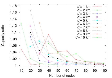
Figure 4: Average value of the capacity ratio $\chi^{\prime}_{\mathrm{phys}}(G)/\chi^{\prime*}_{\mathrm{phys}}(G)$ over the graph instances $G$ in Table 1 for which $\chi^{\prime*}_{\mathrm{phys}}(G)<\chi^{\prime}_{\mathrm{phys}}(G)$ (i.e., those accounted for in Figure 3). Confidence intervals are shown separately in Figure 5, for the sake of clarity.

Another observable of interest is the ratio of capacity improvement, given by $\chi_{\mathrm{phys}}^{\prime}(G)/\chi_{\mathrm{phys}}^{\prime*}(G)$, for those instances $G$ for which $\chi_{\mathrm{phys}}^{\prime*}(G)<\chi_{\mathrm{phys}}^{\prime}(G)$ is obtained. This is shown in Figure 4 as averages over the instances accounted for in Figure 3, with relative confidence intervals shown separately in Figure 5 (for clarity’s sake). A relationship continues to exist between the graphs’ node densities and their capacity gains, but unlike the case of Figure 4, now the trend is for the lower-node-density graphs to afford higher capacity gains. This can be seen as we fix $d$ and increase $|N|$ (plots in the figure are generally decreasing toward $1$) and, to a limited extent, across values of $d$ as well. What prevents us from stating the latter more firmly is the way the plots in Figure 4 deviate from what they would look like ideally (plots nicely nested one above the other with increasing $d$). This may have to do with the higher confidence intervals occurring precisely where deviations from the said ideal are most striking (confidence intervals up to nearly $7\%$ of the corresponding means in some cases; cf. Figure 5), but only further experimentation will clarify the issue.

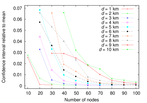
Figure 5: Confidence intervals corresponding to the data in Figure 4. Intervals are given at the $95\%$ level as fractions of the corresponding means.

5 Concluding remarks

In this paper we have addressed the problem of maximizing the capacity of wireless mesh networks by scheduling its links optimally for operation in the physical interference model. We have modeled the network as an undirected graph $G$ and cast the scheduling problem as the problem of coloring the edges of $G$.

In the simpler, protocol-based interference model, the customary approach is to define network capacity as $1/\chi^{\prime}(G)$, where $\chi^{\prime}(G)$ is the chromatic index of $G$ (i.e., the minimum number of colors with which $G$’s edges can be colored with one color per edge, provided no two edges sharing an end vertex get the same color). By redefining network capacity as $1/\chi^{\prime*}(G)$, where $\chi^{\prime*}(G)$ is the fractional chromatic index of $G$, and noting that $\chi^{\prime*}(G)\leq\chi^{\prime}(G)$ necessarily, it becomes possible to aim for higher network capacity as links are scheduled for operation. Fractional coloring differs from integer coloring in that edges are allowed to receive more than one color, the same number of colors for all edges, and also in that optimality is now defined as minimizing the ratio $\chi^{\prime k}(G)/k$ for $k\geq 1$, where $\chi^{\prime k}(G)$ is the minimum number of colors required to color the edges of $G$ in such a way that every edge gets $k$ colors.

Finding $\chi^{\prime*}(G)$ can be approached via the solution of an LP problem based on knowing the set $\mathcal{M}$ of all matchings of graph $G$. This makes the transition to the physical interference model straightforward by simply letting $\mathcal{M}$ contain only those matchings that are feasible as defined for the model. Concentrating on this restricted set of matchings led to the definition of a new fractional chromatic index for $G$, $\chi^{\prime*}_{\mathrm{phys}}(G)$, and correspondingly a new definition of network capacity, $1/\chi^{\prime*}_{\mathrm{phys}}(G)$. Notably, the single-color-per-edge definitions of network capacity, $1/\chi^{\prime}(G)$ for the protocol-based interference model, $1/\chi^{\prime}_{\mathrm{phys}}(G)$ for the physical interference model, are not eliminated by the new definitions. Instead, they are simply subsumed, because they correspond to the $k=1$ cases and can therefore be optimal whenever $\chi^{\prime*}(G)=\chi^{\prime}(G)$ or $\chi^{\prime*}_{\mathrm{phys}}(G)=\chi^{\prime}_{\mathrm{phys}}(G)$, respectively.

Our computational experiments on the physical interference model do confirm that this can happen relatively often. On the other hand, they also reveal that, particularly in the case of denser networks (larger number of nodes per unit area), occurrences of $\chi^{\prime*}_{\mathrm{phys}}(G)<\chi^{\prime}_{\mathrm{phys}}(G)$ happen as well and sometimes account for non-negligible capacity improvements (i.e., increases in the ratio $\chi^{\prime}_{\mathrm{phys}}(G)/\chi^{\prime*}_{\mathrm{phys}}(G)$). Be that as it may, adopting the fractional-coloring framework allows optimization to be carried out exclusively by solving the corresponding LP problem, without any need whatsoever to call upon the ILP problem that accompanies it. As we remarked in Section 3, solving the latter is in general substantially more time-consuming.

We close with further remarks on issues that were left open in the previous sections.

5.1 Multigraph representation of the network

As we remarked in Section 2, representing the network by the undirected graph $G$ precludes any two nodes from participating together in more than one link, even in two “antiparallel” links (i.e., two links $e,f$ in which one of the nodes serves as sender in $e$ and receiver in $f$, the other node as sender in $f$ and receiver in $e$). This representational difficulty can be easily resolved by resorting to a multigraph instead of a graph, i.e., by allowing two vertices to be joined by multiple edges.

The consequence of this for our formulation in Section 2 would be simply to increase the size of the matching set $\mathcal{M}$. In fact, if we denote this set by $\mathcal{M}_{1}$ when all edges have unit multiplicities and by $\mathcal{M}_{\mathrm{mult}}$ when a general multiplicity $m_{e}$ is allowed for each edge $e\in L$, then the effect would be an increase in the overall number of matchings from $|{\mathcal{M}_{1}}|=\sum_{M\in\mathcal{M}_{1}}1$ to $|\mathcal{M}_{\mathrm{mult}}|=\sum_{M\in\mathcal{M}_{1}}\prod_{e\in M}m_{e}$.

5.2 Regarding scalability

It is clear from our discussion in Section 4 that the networks we experimented with were limited by the need to enumerate all feasible matchings in $\mathcal{M}$ in order to exactly solve the LP problem given by Eqs. (2)–(4) and the ILP problem given by Eqs. (12)–(14). The number of such matchings eventually exhausts all computational resources available, thus making it impossible for $\mathcal{M}$ to be enumerated and for either problem to be solved. Ultimately, however, it is the LP problem that matters most, and for this one a clear path exists for the search for scalability.

To see that a substantially more efficient alternative may be available, consider the particular case mentioned at the beginning of Section 2.2, in which $\mathcal{M}$ is the set of all matchings of $G$ (i.e., not necessarily feasible in the sense of the physical interference model). In this case, the better alternative is to consider the LP problem in its dual formulation, given as follows.

maximize $$\textstyle z=\sum_{e\in L}y_{e}$$ (15)

subject to $$\textstyle\sum_{e\in M}y_{e}\leq 1. \forall M\in\mathcal{M}$$ (16)

In this formulation, for each $e\in L$ we have a real variable $y_{e}$ (which can be negative, zero, or positive, by virtue of the equality constraint in Eq. (4)), and for each matching $M\in\mathcal{M}$ we have a constraint forbidding the $y_{e}$’s for $e\in M$ to add up to more than $1$ (Eq. (16)). The goal is to maximize the sum of all $y_{e}$’s (the objective function $z$ in Eq. (15)). By LP duality, if the LP problem in Eqs. (2)–(4) defines the fractional chromatic index of $G$, then so does the one in Eqs. (15) and (16).

It would seem that the new formulation suffers from the same problem as the previous one, the only difference being that now the size of $\mathcal{M}$ is reflected in the number of constraints, not the number of variables. While the latter is clearly true, it is in principle possible to solve the problem without listing all constraints explicitly. We start by maximizing $z$ subject to only a minimal set of constraints (one for each singleton matching $\{e\}\subseteq L$, which ensures a finite maximum value for $z$). Then we iterate, each time expanding the set of explicitly listed constraints with the addition of an unlisted one that is currently violated. We do this until no violated unlisted constraints remain.

In order to succeed with this approach, we must ensure that both the time required to identify a violated unlisted constraint and the overall number of iterations are polynomially bounded. The first of these goals is achieved by resorting to the problem of finding a maximum-weight matching in $G$, which is known to be solvable in polynomial time by a variety of methods (cf., e.g., [44] and references therein). To see how this problem can be of use, let $y_{e}^{*}$ be the value of $y_{e}$ for each $e\in L$ after one of the iterations and find a maximum-weight matching of $G$ with the $y_{e}^{*}$’s as weights. Let $M^{*}$ be the matching obtained, of weight $W^{*}=\sum_{e\in M^{*}}y_{e}^{*}$. If $W^{*}>1$, then clearly the constraint in Eq. (16) for $M=M^{*}$ is being violated and should therefore be listed explicitly for the next iteration. If $W^{*}\leq 1$, then clearly no further violated constraints exist (since $M^{*}$ has maximum weight) and no further iterations are needed. As for the second goal, that of iterating for only a polynomially-bounded number of times, the ellipsoid method for linear programming, though impractical, provides the necessary guarantee [45]. An essentially equivalent path is followed in [22].

The case in which the matchings in $\mathcal{M}$ are all feasible in the sense of the physical interference model is substantially more complex, but at least we have the results of [45] to rely on for guidance. Specifically, what we must do is discover a polynomial-time algorithm to find a maximum-weight feasible matching of $G$. Such an algorithm will depend on all the intricacies underlying the definition of SINR in Eq. (1), and whether one exists is for now an open problem. Should it not exist, or should it prove too elusive to find, a more costly algorithm will also do: though requiring more computational effort to determine the required feasible matching, the expected savings derived from not having to list a huge number of constraints explicitly are bound to be worth the additional resources it expends.

Acknowledgments

We acknowledge partial support from Conselho Nacional de Desenvolvimento Científico e Tecnológico (CNPq), Coordenação de Aperfeiçoamento de Pessoal de Nível Superior (CAPES), and a BBP grant from Fundação Carlos Chagas Filho de Amparo à Pesquisa do Estado do Rio de Janeiro (FAPERJ).

References

- [1] P. Gupta and P. R. Kumar. The capacity of wireless networks. IEEE T. Inform. Theory, 46:388–404, 2000.
- [2] K. Jain, J. Padhye, V. N. Padmanabhan, and L. Qiu. Impact of interference on multi-hop wireless network performance. In Proc. MobiCom 2003, pages 66–80, 2003.
- [3] G. Brar, D. M. Blough, and P. Santi. Computationally efficient scheduling with the physical interference model for throughput improvement in wireless mesh networks. In Proc. MobiCom 2006, pages 2–13, 2006.
- [4] D. M. Blough, G. Resta, and P. Santi. Approximation algorithms for wireless link scheduling with SINR-based interference. IEEE/ACM T. Network., 18:1701–1712, 2010.
- [5] W. Wang, Y. Wang, X.-Y. Li, W.-Z. Song, and O. Frieder. Efficient interference-aware TDMA link scheduling for static wireless networks. In Proc. MobiCom 2006, pages 262–273, 2006.
- [6] T. Moscibroda, Y. A. Oswald, and R. Wattenhofer. How optimal are wireless scheduling protocols? In Proc. INFOCOM 2007, pages 1433–1441, 2007.
- [7] D. Chafekar, V. S. A. Kumart, M. V. Marathe, S. Parthasarathy, and A. Srinivasan. Approximation algorithms for computing capacity of wireless networks with SINR constraints. In Proc. INFOCOM 2008, pages 1166–1174, 2008.
- [8] Q.-S. Hua and F. C. M. Lau. Exact and approximate link scheduling algorithms under the physical interference model. In Proc. DIALM-FOMC 2008, pages 45–54, 2008.
- [9] O. Goussevskaia, R. Wattenhofer, M. M. Halldorsson, and E. Welzl. Capacity of arbitrary wireless networks. In Proc. INFOCOM 2009, pages 1872–1880, 2009.
- [10] P. Santi, R. Maheshwari, G. Resta, S. Das, and D. M. Blough. Wireless link scheduling under a graded SINR interference model. In Proc. FOWANC 2009, pages 3–12, 2009.
- [11] D. Yang, X. Fang, N. Li, and G. Xue. A simple greedy algorithm for link scheduling with the physical interference model. In Proc. GLOBECOM 2009, pages 4572–4577, 2009.
- [12] C. Boyaci, B. Li, and Y. Xia. An investigation on the nature of wireless scheduling. In Proc. INFOCOM 2010, pages 1–9, 2010.
- [13] D. Yang, X. Fang, G. Xue, A. Irani, and S. Misra. Simple and effective scheduling in wireless networks under the physical interference model. In Proc. GLOBECOM 2010, pages 1–5, 2010.
- [14] C. H. P. Augusto, C. B. Carvalho, M. W. R. da Silva, and J. F. de Rezende. REUSE: a combined routing and link scheduling mechanism for wireless mesh networks. Comput. Commun., 34:2207–2216, 2011.
- [15] M. Leconte, J. Ni, and R. Srikant. Improved bounds on the throughput efficiency of greedy maximal scheduling in wireless networks. IEEE/ACM T. Network., 19:709–720, 2011.
- [16] Y. Shi, Y. T. Hou, S. Kompella, and H. D. Sherali. Maximizing capacity in multihop cognitive radio networks under the SINR model. IEEE T. Mobile Comput., 10:954–967, 2011.
- [17] O. Goussevskaia, M. M. Halldorsson, and R. Wattenhofer. Algorithms for wireless capacity. IEEE/ACM T. Network., 22:745–755, 2014.
- [18] M. Nabli, F. Abdelkefi, W. Ajib, and M. Siala. Efficient centralized link scheduling algorithms in wireless mesh networks. In Proc. IWCMC 2014, pages 660–665, 2014.
- [19] C. Wang, J. Yu, D. Yu, B. Huang, and S. Yu. An improved approximation algorithm for the shortest link scheduling in wireless networks under SINR and hypergraph models. J. Comb. Optim., 32:1052–1067, 2016.
- [20] Z.-A. Zhou and C.-G. Li. Approximation algorithms for maximum link scheduling under SINR-based interference model. Int. J. Distr. Sens. Netw., 2015:120812, 2015.
- [21] F. R. J. Vieira, J. F. de Rezende, and V. C. Barbosa. Scheduling wireless links by vertex multicoloring in the physical interference model. Comput. Netw., 99:125–133, 2016.
- [22] B. Hajek and G. Sasaki. Link scheduling in polynomial time. IEEE T. Inform. Theory, 34:910–917, 1988.
- [23] R. L. Cruz and A. V. Santhanam. Optimal routing, link scheduling and power control in multihop wireless networks. In Proc. INFOCOM 2003, pages 702–711, 2003.
- [24] M. Alicherry, R. Bhatia, and L. Li. Joint channel assignment and routing for throughput optimization in multi-radio wireless mesh networks. In Proc. MobiCom 2005, pages 58–72, 2005.
- [25] J. Wang, P. Du, W. Jia, L. Huang, and H. Li. Joint bandwidth allocation, element assignment and scheduling for wireless mesh networks with MIMO links. Comput. Commun., 31:1372–1384, 2008.
- [26] A. Capone, G. Carello, I. Filippini, S. Gualandi, and F. Malucelli. Routing, scheduling and channel assignment in wireless mesh networks: optimization models and algorithms. Ad Hoc Netw., 8:545–563, 2010.
- [27] A. D. Gore and A. Karandikar. Link scheduling algorithms for wireless mesh networks. IEEE Comm. Surv. Tutor., 13:258–273, 2011.
- [28] T. Kesselheim. A constant-factor approximation for wireless capacity maximization with power control in the SINR model. In Proc. SODA 2011, pages 1549–1559, 2011.
- [29] P.-J. Wan, O. Frieder, X. Jia, F. Yao, X. Xu, and S. Tang. Wireless link scheduling under physical interference model. In Proc. INFOCOM 2011, pages 838–845, 2011.
- [30] I. Rubin, C.-C. Tan, and R. Cohen. Joint scheduling and power control for multicasting in cellular wireless networks. EURASIP J. Wirel. Comm., 2012:250, 2012.
- [31] F. R. J. Vieira, J. F. de Rezende, V. C. Barbosa, and S. Fdida. Scheduling links for heavy traffic on interfering routes in wireless mesh networks. Comput. Netw., 56:1584–1598, 2012.
- [32] R. Mathar and T. Niessen. Optimum positioning of base stations for cellular radio networks. Wirel. Netw., 6:421–428, 2000.
- [33] C. Prommak, J. Kabara, D. Tipper, and C. Charnsripinyo. Next generation wireless LAN system design. In Proc. MILCOM 2002, volume 1, pages 473–477, 2002.
- [34] P. Wertz, M. Sauter, F. M. Landstorfer, G. Wölfle, and R. Hoppe. Automatic optimization algorithms for the planning of wireless local area networks. In Proc. VTC 2004, pages 3010–3014, 2004.
- [35] A. Bahri and S. Chamberland. On the wireless local area network design problem with performance guarantees. Comput. Netw., 48:856–866, 2005.
- [36] L. Narayanan. Channel assignment and graph multicoloring. In I. Stojmenovic, editor, Handbook of Wireless Networks and Mobile Computing, pages 71–94. John Wiley & Sons, New York, NY, 2002.
- [37] K. I. Aardal, S. P. M. van Hoesel, A. M. C. A. Koster, C. Mannino, and A. Sassano. Models and solution techniques for frequency assignment problems. Ann. Oper. Res., 153:79–129, 2007.
- [38] M. Stiebitz, D. Scheide, B. Toft, and L. M. Favrholdt. Graph Edge Coloring. Wiley, Hoboken, NJ, 2012.
- [39] S. Fiorini and R. J. Wilson. Edge-Colourings of Graphs. Pitman, London, UK, 1977.
- [40] S. Stahl. Fractional edge colorings. Cah. C.E.R.O., 21:127–131, 1979.
- [41] E. R. Scheinerman and D. H. Ullman. Fractional Graph Theory. Wiley, New York, NY, 1997.
- [42] J. A. Bondy and U. S. R. Murty. Graph Theory. Springer-Verlag, London, UK, 2008.
- [43] A. Schrijver. Combinatorial Optimization, volume A. Springer-Verlag, Berlin, Germany, 2003.
- [44] C.-C. Huang and T. Kavitha. New algorithms for maximum weight matching and a decomposition theorem. Math. Oper. Res., 42:411–426, 2017.
- [45] M. Grötschel, L. Lovász, and A. Schrijver. The ellipsoid method and its consequences in combinatorial optimization. Combinatorica, 1:169–197, 1981.