Complete integration-by-parts reductions of the non-planar hexagon-box via module intersections

Abstract

We present the powerful module-intersection integration-by-parts (IBP) method, suitable for multi-loop and multi-scale Feynman integral reduction. Utilizing modern computational algebraic geometry techniques, this new method successfully trims traditional IBP systems dramatically to much simpler integral-relation systems on unitarity cuts. We demonstrate the power of this method by explicitly carrying out the complete analytic reduction of two-loop five-point non-planar hexagon-box integrals, with degree-four numerators, to a basis of $73$ master integrals.

MITP/18-034

UUITP-16/18

1 Introduction

High precision in the theoretical predictions for cross sections is necessary for the analysis of the Large Hadron Collider (LHC) Run II experiments. For many processes, the next-to-next-to-leading-order (NNLO) contributions are needed for precision-level predictions. NNLO in general requires the computation of a large number of two-loop (or, in some cases, higher-loop) Feynman integrals, which is often a bottleneck problem for particle physics.

Integration-by-parts (IBP) reduction is a key tool to reduce the large number of multi-loop Feynman integrals to a small integral basis of so-called master integrals. Schematically, for an $L$-loop integral in dimensional regularization with the inverse propagators $D_{1},\ldots,D_{m}$, we have

$$0=\int\frac{{\rm d}^{D}\ell_{1}}{\mathrm{i}\pi^{D/2}}\ldots\frac{{\rm d}^{D}\ell_{L}}{\mathrm{i}\pi^{D/2}}\sum_{j=1}^{L}\frac{\partial}{\partial\ell_{j}^{\mu}}\frac{v_{j}^{\mu}\hskip 1.42262pt}{D_{1}^{\nu_{1}}\cdots D_{m}^{\nu_{m}}}\,,$$ (1.1)

where the $v_{j}^{\mu}$ are vectors constructed from the external momenta and the loop momenta. Expanding the action of the derivative in eq. (1.1) leads to an IBP identity, which is a linear relation between multi-loop Feynman integrals. After collecting a sufficient set of IBP identities, one can carry out reduced row reduction in a specific integral ordering to express a target set of integrals as a linear combination of the master integrals.

The row reduction of IBP identities can be achieved by the Laporta algorithm Laporta:2000dc ; Laporta:2001dd . There are several publicly available implementations of IBP reductions: AIR Anastasiou:2004vj , FIRE Smirnov:2008iw ; Smirnov:2014hma , Reduze Studerus:2009ye ; vonManteuffel:2012np , LiteRed Lee:2012cn , Kira Maierhoefer:2017hyi , as well as various private implementations. In the standard Laporta algorithm and many of its variants, integrals with doubled propagators appear in the intermediate steps and also in the master integral basis. To trim the linear system of IBP identities for row reduction, one may impose the condition that no integrals with doubled propagators appear in the IBP identities Gluza:2010ws . This condition can be solved by the syzygy computation Gluza:2010ws or linear algebra Schabinger:2011dz . In refs. Ita:2015tya ; Larsen:2015ped , methods for deriving IBP reductions on generalized-unitarity cuts was introduced. IBP reduction can also be sped up by the finite-field sampling method vonManteuffel:2014ixa . For several multiple-scale Feynman integrals, inspired choices of IBP generating vectors $v_{j}^{\mu}$, leading to simple IBP identities, can be obtained from dual conformal symmetry Bern:2017gdk . In a recent development, IBP identities which target integrals with arbitrary-degree numerators Kosower:2018obg were introduced. An initial (and simpler) step to carrying out the IBP reductions is that of determining the integral basis itself. This can be done by the packages Mint Lee:2013hzt or Azurite Georgoudis:2016wff . The dimension of the integral basis can be efficiently determined by the computation of an Euler characteristic which naturally arises in the D-module theory of polynomial annihilators Bitoun:2017nre .

IBP reductions, combined with generalized-unitarity methods Britto:2004nc ; Britto:2005fq ; Kosower:2011ty ; Johansson:2012zv or integrand reduction methods Ossola:2006us ; Badger:2012dp ; Zhang:2012ce ; Mastrolia:2012an , have led to successful computations of many complicated multi-loop integrands. Furthermore, IBP reductions are also important for setting up the differential equations for Feynman integrals Kotikov:1990kg ; Kotikov:1991pm ; Bern:1993kr ; Remiddi:1997ny ; Gehrmann:1999as ; Henn:2013pwa ; Papadopoulos:2014lla ; Lee:2014ioa ; Ablinger:2015tua ; Papadopoulos:2015jft ; Liu:2017jxz , which has proven a highly efficient method for evaluating Feynman integrals. Recent developments in multi-loop integral reduction and the differential equation method have produced very impressive results for the two-loop amplitudes of $2\to 3$ scattering processes with the all-plus-helicity configuration Badger:2013gxa ; Badger:2015lda ; Gehrmann:2015bfy and the generic-helicity configuration Badger:2017jhb ; Abreu:2017hqn ; Boels:2018nrr . IBP reductions are also crucial for deriving dimension recursion relations Tarasov:1996br ; Lee:2009dh ; Lee:2010wea .

For multi-loop, high-multiplicity or multi-scale amplitude computations, the IBP reductions frequently become the bottleneck which requires extensive computing resources and time. Schematically, the complexity of IBP reductions mainly originate from the following facts,

1. Multi-loop IBP identities involve many contributing integrals, and the complexity of row reduction grows quickly with the number of integrals.

2. There are many external invariants (i.e., Mandelstam variables and mass parameters), and the algebraic computation of polynomials or rational functions in these parameters requires a substantial amount of CPU time and RAM.

In this paper, utilizing our new powerful module-intersection IBP reduction method, we present solutions to the above problems:

1. With the module-intersection computation Zhang:2016kfo , we dramatically reduce the number of relevant IBP identities and integrals involved by imposing the no-doubled-propagator condition and applying unitarity cuts.

2. With the classical technique of treating parameters as new variables and imposing a special monomial ordering, originating from primary decomposition algorithms GTZ in commutative algebra, we can efficiently compute analytic IBP reductions with many parameters.

In this paper, we demonstrate our method by treating the cutting-edge example of the analytic IBP reduction of two-loop five-point non-planar hexagon-box integrals, with all degree-$1,2,3,4$ numerators, to the basis of $73$ master integrals. This computation was carried out using private implementations in Singular Singular and Mathematica of the ideas presented in this paper. Our result of fully analytic IBP reductions can be downloaded from,

https://github.com/yzhphy/hexagonbox_reduction/releases/download/1.0.0/hexagon_box_degree_4_Final.zip  .

This paper is organized as follows. In section 2 we present our module-intersection method for trimming IBP systems and describe a simple way of obtaining the individual modules needed for our method. In section 3, the central part of our paper, we present a highly efficient new method for computing these intersections. We then explain the technical details of performing row reduction for the trimmed IBP systems from module intersections in section 4. In section 5, we present our example, the module-intersection IBP reduction of hexagon-box integrals, in details. The conclusions and outlook are given in section 6.

2 Simplification of IBP systems by module-intersection method

In this section we present the details on trimming IBP systems by requiring the absence of integrals with doubled propagators Gluza:2010ws , and by furthermore applying unitarity cuts. To demonstrate our method clearly, we first explain how to efficiently impose the no-doubled-propagator condition without applying unitarity cuts. Then we show that the same approach can be applied on unitarity cuts. In both cases, the algebraic constraints for trimming IBP systems are reformulated as the problem of computing the intersection of two modules over a polynomial ring Zhang:2016kfo . At the end of this section, the algorithm for computing each individual module is introduced, while the intersection algorithm, the heart of this method, will be introduced in section 3.

2.1 Module intersection method without unitarity cuts

The objects under consideration are the multi-loop Feynman integrals,

$$I(\nu_{1},\ldots,\nu_{m})=\int\frac{{\rm d}^{D}l_{1}}{i\pi^{D/2}}\ldots\frac{{\rm d}^{D}l_{L}}{i\pi^{D/2}}\frac{1}{D_{1}^{\nu_{1}}\cdots D_{m}^{\nu_{m}}}\,.$$ (2.1)

Here $\nu_{i}\in\mathbb{Z}$, $l_{1},\ldots,l_{L}$ denote the loop momenta, and $p_{1},\ldots,p_{E}$ the independent external momenta. By the procedure of integrand reduction, we can set $m=L(L+1)/2+LE$. The $D_{i}$ denote inverse propagators.

To study IBP reduction of integrals of the form (2.1), we focus on the family of Feynman integrals associated with a particular Feynman diagram with $k$ propagators (where $k\leq m$) and all its daughter diagrams, obtained by pinching propagators. Without loss of generality, the inverse denominators of this Feynman diagram can be labeled as $D_{1},\ldots,D_{k}$. Therefore, the family of integrals is,

$$\mathcal{F}=\{I(\nu_{1},\ldots,\nu_{m})\hskip 2.84526pt|\quad\nu_{j}\leq 0\text{ if }j>k\}\,.$$ (2.2)

Traditionally, IBP reduction is carried out within such a family. However, since the majority of the Feynman integrals that contribute to a quantity in perturbative QFT are integrals without doubled propagators, it is natural to consider the subfamily

$$\mathcal{F}_{\mathrm{ndp}}=\{I(\nu_{1},\ldots,\nu_{m})\hskip 2.84526pt|\quad\nu_{j}\leq 1\text{ if }j\leq k,\quad\nu_{j}\leq 0\text{ if }j>k\}$$ (2.3)

and the IBP relations for integrals in this subfamily Gluza:2010ws .

We find that it is convenient to use the Baikov representation Baikov:1996rk of Feynman integrals for their integration-by-parts (IBP) reduction for several reasons: 1) the integrand reduction is manifest in this representation, 2) it is easy to apply unitarity cuts, 3) most importantly, it is surprisingly simple to trim IBP systems analytically in this representation. Here we briefly review the Baikov representation.

We collect the external and internal momenta as,

$$V=(v_{1},\ldots,v_{E+L})=(p_{1},\ldots,p_{E},\ell_{1},\ldots,\ell_{L})\,.$$ (2.4)

The Gram matrix $S$ of these vectors is,

$$S=\left(\begin{array}[]{ccc|ccc}x_{1,1}&\cdots&x_{1,E}&x_{1,E+1}&\cdots&x_{1,E+L}\\ \vdots&\ddots&\vdots&\vdots&\ddots&\vdots\\ x_{E,1}&\cdots&x_{E,E}&x_{E,E+1}&\cdots&x_{E,E+L}\\ \hline\cr x_{E+1,1}&\cdots&x_{E+1,E}&x_{E+1,E+1}&\cdots&x_{E+1,E+L}\\ \vdots&\ddots&\vdots&\vdots&\ddots&\vdots\\ x_{E+L,1}&\cdots&x_{E+L,E}&x_{E+L,E+1}&\cdots&x_{E+L,E+L}\end{array}\right)\,,$$ (2.5)

where the elements are defined as $x_{i,j}=v_{i}\cdot v_{j}$. The upper-left $E\times E$ block is the Gram matrix of the external momenta, which is denoted as $G$. Defining $z_{i}\equiv D_{i}$ and integrating out solid-angle directions, the Feynman integral (2.1) takes the following form in Baikov representation,

$$I(\nu_{1},\ldots,\nu_{m})\hskip 1.42262pt =\hskip 1.42262ptC_{E}^{L}\hskip 1.99168ptU^{\frac{E-D+1}{2}}\int{\rm d}z_{1}\cdots{\rm d}z_{m}P^{\frac{D-L-E-1}{2}}\frac{1}{z_{1}^{\nu_{1}}\cdots z_{m}^{\nu_{m}}}\,,$$ (2.6)

where $P\equiv\det S$, $U\equiv\det G$, and the factor $C_{E}^{L}$ originates from the solid-angle integration and the Jacobian for the transformation $x_{i,j}\to z$. For the derivation of IBP identities, $U$ and $C_{E}^{L}$ are irrelevant, so we may ignore them in the following discussion. Note that in this representation, the inverse denominators $D_{i}$ become free variables, and so the integrand reduction can be done automatically.

An IBP identity in this representation reads,

$$0 =\int{\rm d}z_{1}\cdots{\rm d}z_{m}\sum_{i=1}^{m}\frac{\partial}{\partial z_{i}}\bigg{(}a_{i}P^{\frac{D-L-E-1}{2}}\frac{1}{z_{1}^{\nu_{1}}\cdots z_{m}^{\nu_{m}}}\bigg{)}$$

$$=\int{\rm d}z_{1}\cdots{\rm d}z_{m}\sum_{i=1}^{m}\bigg{(}\frac{\partial a_{i}}{\partial z_{i}}+\frac{D-L-E-1}{2P}a_{i}\frac{\partial P}{\partial z_{i}}-\frac{\nu_{i}a_{i}}{z_{i}}\bigg{)}P^{\frac{D-L-E-1}{2}}\frac{1}{z_{1}^{\nu_{1}}\cdots z_{m}^{\nu_{m}}}\,.$$ (2.7)

Here the $a_{i}$ denote polynomials in the ring $\mathbb{A}=\mathbb{Q}(\mathbf{s})[z_{1},\ldots,z_{m}]$. (We use $\mathbf{s}$ to represent the independent Mandelstam variables and mass parameters collectively.) We remark that in the Baikov representation, the Baikov polynomial $P$ vanishes on the boundary of the integration domain, and hence there is no surface term in the IBP identity. Note that the terms with the pole $1/P$ appearing inside the parenthesis in eq. (2.7) correspond to dimension-shifted integrals, and as such are not favorable in deriving simple IBP relations. To avoid such poles, we may impose the following constraints on the $a_{i}$ Lee:2014tja ; Ita:2015tya ; Larsen:2015ped ,

$$\bigg{(}\sum_{i=1}^{m}a_{i}\frac{\partial P}{\partial z_{i}}\bigg{)}+bP=0\,,$$ (2.8)

where $b$ is also required to be a polynomial in $\mathbb{A}$. This constraint is known in computational commutative algebra as a “syzygy” equation Gluza:2010ws . In the following discussion, we only focus on the polynomials $a_{i}$, since once they are known it is straightforward to recover the polynomial $b$. The solutions of eq. (2.8), taking the form,

$$(a_{1},\ldots,a_{m})$$ (2.9)

form a sub-module of the polynomial module $\mathbb{A}^{m}$, which we denote $M_{1}$ in the following.

Furthermore, to trim the IBP system, it is possible to work with integrals in $\mathcal{F}_{\mathrm{ndp}}$, i.e. integrals without doubled propagators Gluza:2010ws . Note from the second line of eq. (2.7) that, even if the integral inside the differential operator has $\nu_{i}\leq 1$, the derivative will produce integrals with doubled propagators. This can also be prevented by a suitable choice of the $a_{i}$. For example, if we consider the integral of the parent diagram, $\nu_{1}=\cdots=\nu_{k}=1$, $\nu_{k+1}\leq 0,\ldots,\nu_{m}\leq 0$ inside eq. (2.7), we can avoid doubled propagators by requiring that $a_{i}$ is divisible by $z_{i}$,

$$a_{i}=b_{i}z_{i}\,,\quad i=1,\ldots,k\,.$$ (2.10)

Such $(a_{1},\ldots,a_{m})$ also form a sub-module of $\mathbb{A}^{m}$, which we denote $M_{2}$. We need to solve eqs. (2.8) and (2.10) simultaneously to find IBP relations which involve neither dimension shifts nor doubled propagators in Baikov representation.

The strategy in ref. Larsen:2015ped to solve these conditions is to replace $a_{i}$ by $b_{i}$ in eq. (2.8) and then solve for $(b_{1},\ldots,b_{k},a_{k+1},\ldots,a_{m},b)$ as a single syzygy equation, employing Schreyer’s theorem. However, this approach, although it works well for simple two-loop four-point integrals, becomes less practical for more complicated kinematics. It was suggested in the reference Zhang:2016kfo that a better strategy is to determine the generators of $M_{1}$ and $M_{2}$ individually, and then calculate the module intersection,

$$M_{1}\cap M_{2}\,,$$ (2.11)

whose generators are solutions of eqs. (2.8) and (2.10). Geometrically, elements in $M_{1}\cap M_{2}$ are the polynomial tangent vectors of the reducible hypersurface Hauser1993 ; Zhang:2016kfo

$$z_{1}\ldots z_{k}P=0\,.$$ (2.12)

In subsection 2.3, we will see that it takes no effort to find the generators of $M_{1}$ and $M_{2}$. In section 3 we present a highly efficient algorithm for computing the intersection $M_{1}\cap M_{2}$.

Once eqs. (2.8) and (2.10) are solved, we obtain the simplified IBP identities without doubled propagators. They take the following form,

$$0=\int{\rm d}z_{1}\cdots{\rm d}z_{m}\bigg{(}\sum_{i=1}^{m}\frac{\partial a_{i}}{\partial z_{i}}-\sum_{i=1}^{k}b_{i}-\sum_{i=k+1}^{m}\frac{\nu_{i}a_{i}}{z_{i}}-\frac{D-L-E-1}{2}b\bigg{)}\frac{P^{\frac{D-L-E-1}{2}}}{z_{1}\ldots z_{k}z_{k+1}^{\nu_{k+1}}\ldots z_{m}^{\nu_{m}}}\,.$$ (2.13)

Once the generators of $M_{1}\cap M_{2}$ are obtained, we multiply them by monomials in the $z_{i}$ in order to get a spanning set of IBP identities for the reduction targets. Alternatively, it is possible to apply D-module theory to get the IBP reductions directly from the generators of $M_{1}\cap M_{2}$. We leave this direction for future research.

2.2 Module intersection method with cuts

In practice, for Feynman diagrams with high multiplicity or high loop order, instead of working with the Feynman integrals directly, it is more convenient to apply unitarity cuts Ita:2015tya ; Larsen:2015ped . In this section we show how to apply the module intersection method in combination with unitarity cuts, thus simplifying the construction and subsequent Gaussian elimination of the IBP identities. We follow the notation of ref. Boehm:2017wjc .

Consider the $c$-fold cut of eq. (5.2) with $c\leq k$. Let $\mathcal{S}_{\mathrm{cut}}$, $\mathcal{S}_{\mathrm{uncut}}$ and $\mathcal{S}_{\mathrm{ISP}}$ denote the sets of indices of cut propagators, uncut propagators and irreducible scalar products (ISP) respectively. Explicitly,

$$\mathcal{S}_{\mathrm{cut}}=\{\zeta_{1},\ldots,\zeta_{c}\}\,,\quad\mathcal{S}_{\mathrm{uncut}}=\{r_{1},\ldots,r_{k-c}\}\,,\quad\mathcal{S}_{\mathrm{ISP}}=\{r_{k-c+1},\ldots,r_{m-c}\}\,.$$ (2.14)

In Baikov represention, the $c$-fold cut of integrals with $\nu_{1}=\cdots=\nu_{k}=1$ takes a simple form,

$$I(\nu_{1},\ldots,\nu_{m})\hskip 1.42262pt \propto\int{\rm d}z_{r_{1}}\cdots{\rm d}z_{r_{m-c}}\frac{\tilde{P}^{\frac{D-L-E-1}{2}}}{z_{r_{1}}\ldots z_{r_{k-c}}z_{r_{k-c+1}}^{\nu_{r_{k-c+1}}}\ldots z_{r_{m-c}}^{\nu_{r_{m-c}}}}\,,$$ (2.15)

where,

$$\tilde{P}\hskip 2.27621pt=\hskip 2.27621ptP|_{z_{\zeta_{1}}\to 0,\ldots,z_{\zeta_{c}}\to 0}\,.$$ (2.16)

We can derive IBP identities for the integrals on the cut $\mathcal{S}_{\mathrm{cut}}$,

$$0 =\int{\rm d}z_{r_{1}}\ldots{\rm d}z_{r_{m-c}}\sum_{i=1}^{m-c}\frac{\partial}{\partial z_{r_{i}}}\bigg{(}\tilde{a}_{r_{i}}\frac{\tilde{P}^{\frac{D-L-E-1}{2}}}{z_{r_{1}}\ldots z_{r_{k-c}}z_{r_{k-c+1}}^{\nu_{r_{k-c+1}}}\ldots z_{r_{m-c}}^{\nu_{r_{m-c}}}}\bigg{)}$$

$$=\int{\rm d}z_{r_{1}}\ldots{\rm d}z_{r_{m-c}}\bigg{(}\sum_{i=1}^{m-c}\frac{\partial\tilde{a}_{r_{i}}}{\partial z_{r_{i}}}+\frac{D-L-E-1}{2\tilde{P}}\sum_{i=1}^{m-c}\tilde{a}_{r_{i}}\frac{\partial\tilde{P}}{\partial z_{r_{i}}}-\sum_{i=1}^{k-c}\frac{\tilde{a}_{r_{i}}}{z_{r_{i}}}-\sum_{i=k-c+1}^{m-c}\frac{\nu_{r_{i}}\tilde{a}_{r_{i}}}{z_{r_{i}}}\bigg{)}$$

$$\hskip 34.1433pt\times\frac{\tilde{P}^{\frac{D-L-E-1}{2}}}{z_{r_{1}}\ldots z_{r_{k-c}}z_{r_{k-c+1}}^{\nu_{r_{k-c+1}}}\ldots z_{r_{m-c}}^{\nu_{r_{m-c}}}}\,,$$ (2.17)

where $\tilde{a}_{r_{i}}$, $i=1,\ldots,m-c$ are polynomials in $\tilde{\mathbb{A}}=\mathbb{Q}(\mathbf{s})[z_{r_{1}},\ldots z_{r_{m-c}}]$. Once again, to derive simple IBP relations without dimension shifts or doubled propagators Ita:2015tya ; Larsen:2015ped , we may impose the conditions,

$$\Big{(}\sum_{i=1}^{m-c}\tilde{a}_{r_{i}}\frac{\partial\tilde{P}}{\partial z_{r_{i}}}\Big{)}+\tilde{b}\tilde{P} =0\,,$$ (2.18)

$$\tilde{a}_{r_{i}} =\tilde{b}_{r_{i}}z_{r_{i}},\quad i=1,\ldots,k-c\,.$$ (2.19)

Again, the module intersection method provides an efficient tool to solve these constraints simultaneously. However, for the purpose of automation, it is useful to make use of the following slight reformulation. Define

$$\tilde{a}_{\zeta_{i}}\equiv 0\,,\quad i=1,\ldots,c\,,$$ (2.20)

Then eqs. (2.18) and (2.19) are formally recast as,

$$\Big{(}\sum_{i=1}^{m}\tilde{a}_{i}\frac{\partial\tilde{P}}{\partial z_{i}}\Big{)}+\tilde{b}\tilde{P} =0\,,$$ (2.21)

$$\tilde{a}_{r_{i}} =\tilde{b}_{r_{i}}z_{r_{i}}\,,\quad i=1,\ldots,k-c\,.$$ (2.22)

By comparing these equations and their counterparts without applied cuts, we observe the following shortcut. Recall that the modules $M_{1}$ and $M_{2}$ defined in the previous subsection are the solution sets for eqs. (2.8) and (2.10) respectively. We define

$$\tilde{M}_{1}=M_{1}|_{z_{\zeta_{1}}\to 0,\ldots,z_{\zeta_{c}}\to 0}\,,\quad\tilde{M}_{2}=M_{2}|_{z_{\zeta_{1}}\to 0,\ldots,z_{\zeta_{c}}\to 0}\,,$$ (2.23)

whereby the $c$-fold cut on the elements of $M_{1}$ and $M_{2}$ has been imposed. Then clearly,

$$\tilde{M}_{1}\cap\tilde{M}_{2}$$ (2.24)

solve the equations (2.21) and (2.22) simultaneously. Note that any element in $(q_{1},\ldots,q_{m})\in M_{2}$ has the property $q_{\zeta_{i}}=h_{\zeta_{i}}z_{\zeta_{i}}$, $i=1,\ldots,c$. After imposing the cut we have,

$$q_{\zeta_{i}}\big{|}_{z_{\zeta_{1}}\to 0,\ldots,z_{\zeta_{c}}\to 0}=0\,,$$ (2.25)

which is consistent with the requirement (2.20). This automates the computation: to obtain $\tilde{M}_{1}$ and $\tilde{M}_{2}$, we first compute $M_{1}$ and $M_{2}$, and then simply apply the rules for the various cuts. An algorithm for computation of the intersection will be introduced in section 3.

Once the constraints (2.21) and (2.22) are solved, the IBP identities on the cut take the simple form,

$$0=\int{\rm d}z_{r_{1}}\cdots{\rm d}z_{r_{m-c}}\ \bigg{(}\sum_{i=1}^{m-c}\frac{\partial\tilde{a}_{r_{i}}}{\partial z_{r_{i}}}-\frac{D-L-E-1}{2}\tilde{b}-\sum_{i=1}^{k-c}\tilde{b}_{r_{i}}-\sum_{i=k-c+1}^{m-c}\frac{\nu_{r_{i}}\tilde{a}_{r_{i}}}{z_{r_{i}}}\bigg{)}$$

$$\times\frac{\tilde{P}^{\frac{D-L-E-1}{2}}}{z_{r_{1}}\ldots z_{r_{k-c}}z_{r_{k-c+1}}^{\nu_{r_{k-c+1}}}\ldots z_{r_{m-c}}^{\nu_{r_{m-c}}}}\,.$$ (2.26)

As for the uncut case, once the generators of $\tilde{M}_{1}\cap\tilde{M}_{2}$ are obtained, we multiply them by monomials in the $z_{r_{i}}$, $i=1,\ldots,m-c$ to get a spanning set of IBP identities.

The cuts necessary for reconstructing the complete IBP identities can be determined from a list of master integrals Larsen:2015ped ; Georgoudis:2016wff : they are the maximal cuts of “uncollapsible” master integrals (master integrals which cannot be obtained from other integrals in the basis by adding propagators). In practice, the list of master integrals can be quickly determined by the packages Mint Lee:2017oca , Azurite Georgoudis:2016wff . The total number of master integrals can also be determined by the D-module theory method of ref. Bitoun:2017nre .

Upon applying Gaussian elimination to the IBP identities evaluated on each cut, we can subsequently merge the obtained reductions to find the complete IBP reductions without applied cuts.

2.3 Algorithm for computing individual modules

The modules $M_{1}$ and $M_{2}$ defined in subsection 2.1, and hence $\tilde{M}_{1}$ and $\tilde{M}_{2}$ defined in the previous subsection, can all be determined without effort.

The condition (2.8) for $M_{1}$ is a syzygy equation for the Baikov polynomial $P$ and its derivatives. Schreyer’s theorem MR1322960 guarantees that solutions for syzygy equations can be obtained from Gröbner basis computations. However, for the Baikov polynomial $P$ this is not necessary, owing to the special structure of $P$. A convenient way to find the solution, or equivalently the tangent vectors for the hypersurface $P=0$, is to use the basic canonical IBP identities Ita:2015tya . Here alternatively, we use the Laplace expansion method Boehm:2017wjc of the Gram determinant $S$ (2.5) to determine $M_{1}$, since the results are manifestly expressed in the $z$ variables.

Laplace expansion of $P=\det S$ yields,

$$\bigg{(}\sum_{k=1}^{E+L}(1{+}\delta_{i,k})x_{j,k}\frac{\partial P}{\partial x_{i,k}}\bigg{)}-2\delta_{i,j}P=0\,,$$ (2.27)

where $E+1\leq i\leq E+L$ and $1\leq j\leq E+L$. These $L(E+L)$ relations are syzygy relations between $P$ and its derivatives in the $x_{i,j}$ variables. It is straightforward to convert them to solutions of eq. (2.8),

$$\sum_{\alpha=1}^{m}(a_{i,j})_{\alpha}\frac{\partial P}{\partial z_{\alpha}}+b_{i,j}P=0\,,$$ (2.28)

where $a_{i,j}$ and $b$ are obtained by applying the chain rule to the expressions in eq. (2.27). Explicitly, they are given by,

$$(a_{i,j})_{\alpha}=\sum_{k=1}^{E+L}(1+\delta_{i,k})\frac{\partial z_{\alpha}}{\partial x_{i,k}}x_{j,k}\hskip 14.22636pt\mathrm{and}\hskip 14.22636ptb_{i,j}=-2\delta_{i,j}\,.$$ (2.29)

It is proven in ref. Boehm:2017wjc via Józefiak complexes Joz78 that the $L(E+L)$ tuples of polynomials $(a_{i,j})_{\alpha}$ form a complete generating set of $M_{1}$.

We remark that,

1. The generating set (2.29) is at most linear in the $z_{i}$.

2. The generating set (2.29) is homogenous in the $z_{i}$ and the Mandelstam variables/mass parameters, as can be inferred from dimensional analysis.

The second property is crucial for our highly efficient algorithm for computing intersections of modules, to be explained in section 3.

The generating set for $M_{2}$ is trivial. There are $m$ generators,

$$z_{1}\mathbf{e}_{1}\,,\quad\ldots,\quad z_{k}\mathbf{e}_{k},\quad\mathbf{e}_{k+1}\,,\quad\ldots,\quad\mathbf{e}_{m}\,.$$ (2.30)

Here $\mathbf{e}_{j}$ is the $j$-th $m$-dimensional unit vector.

The cut cases, $\tilde{M}_{1}$ and $\tilde{M}_{2}$ defined in eq. (2.23), can then be obtained from eqs. (2.29) and (2.30) by simply setting $z_{\zeta_{i}}\to 0$, $i=1,\ldots,c$.

3 Determining the module intersection

In this section, we introduce a highly efficient algorithm for computing generators of the module intersections and an algorithm to trim the generating sets.

Given the two submodules $M_{1},M_{2}\subset A^{t}$ over the multivariate polynomial ring $A=F[z_{1},\ldots,z_{n}]$ with coefficients in the multivariate rational function field $F=\mathbb{Q}(c_{1},\ldots,c_{r})$, our goal is to obtain a generating system of the module $M_{1}\cap M_{2}$ (which is finitely generated since $A$ is Noetherian). We apply Gröbner basis techniques to address this problem. Our algorithms are implemented in the computer algebra system Singular, which focuses on polynomial computations with applications in commutative algebra and algebraic geometry Singular .

We first recall some terminology: Using the notation $z^{\alpha}=z_{1}^{\alpha_{1}}\cdot\ldots\cdot z_{n}^{\alpha_{n}}$ for the monomials in $A$, we call $z^{\alpha}e_{i}$ with a unit basis vector $e_{i}\in A^{t}$ a monomial of $A^{t}$. An $F$-multiple of a monomial is called a term. A monomial ordering on $A^{t}$ is an total ordering $>$ on the set of monomials in $A^{t}$, which respects multiplication, that is, $z^{\alpha}e_{i}>z^{\beta}e_{j}$ implies $z^{\alpha}z^{\gamma}e_{i}>z^{\beta}z^{\gamma}e_{j}$ for all $\alpha,\beta,\gamma,i,j$, and $z^{\alpha}e_{i}>z^{\beta}e_{i}\Leftrightarrow z^{\alpha}e_{j}>z^{\beta}e_{j}$ for all $\alpha,\beta,i,j$. Then $>$ induces a monomial ordering on the monomials of $A$, which we again denote by $>$. In turn, any monomial ordering $>$ on $A$ induces two canonical monomial orderings on $A^{t}$, position over term

$$z^{\alpha}e_{i}>z^{\beta}e_{j}\ :\Longleftrightarrow\ i<j\text{ or (}i=j\text{ and }z^{\alpha}>z^{\beta}\text{)}$$ (3.1)

and analogously term over position. We call a monomial ordering on $A^{t}$ global if the induced ordering on $A$ is global, that is, $z^{\alpha}>1$ for all $\alpha$. Any $0\neq f\in A^{t}$ can be written as $f=c\cdot z^{\alpha}e_{i}+g$ with $z^{\alpha}e_{i}>z^{\beta}e_{j}$ for all terms $\widetilde{c}\cdot z^{\beta}e_{j}$ of $g\in A^{t}$. Then the term $\operatorname{LT}_{>}(f)=c\cdot z^{\alpha}e_{i}$ is called the lead term of $f$, the constant $\operatorname{LC}_{>}(f)=c$ is called the lead coefficient of $f$, and $L_{>}(f)=z^{\alpha}e_{i}$ the lead monomial of $f$. The monomials of $A^{t}$ come with a natural partial order, which we call divisibility

$$z^{\alpha}e_{i}\mid z^{\beta}e_{j}\ \Longleftrightarrow\ i=j\text{ and }z^{\alpha}\mid z^{\beta}.$$ (3.2)

For terms $c_{1}z^{\alpha}e_{i}$ and $c_{2}z^{\beta}e_{j}$ with $z^{\alpha}e_{i}\mid z^{\beta}e_{j}$ we define their quotient as $\frac{c_{2}z^{\beta}e_{j}}{c_{1}z^{\alpha}e_{i}}=\frac{c_{2}z^{\beta}}{c_{1}z^{\alpha}}\in A$. Moreover, we define the least common multiple $\operatorname{lcm}(z^{\alpha}e_{i},z^{\beta}e_{j})$ as zero if $i\neq j$, and as $\operatorname{lcm}(z^{\alpha},z^{\beta})$ otherwise. For a subset $G\subset A^{t}$, the leading module $L(G)$ is the module of all $A$-linear combinations of the lead monomials of the non-zero elements of $G$.

By iteratively canceling the lead term of $f$ via multiples of lead terms of the divisors in $G=\{g_{1},\ldots,g_{l}\}\subset A^{t}$ with respect to a fixed global ordering, we obtain a notion of division with remainder yielding a division expression

$$f=\sum_{i}a_{i}g_{i}+\operatorname*{NF}\nolimits_{>}(f,G)$$ (3.3)

with $a_{i}\in A$ such that $\operatorname*{NF}(0,G)=0$, $\operatorname*{NF}_{>}(f,G)\neq 0$ implies that $L_{>}(\operatorname*{NF}_{>}(f,G))\notin L(G)$, and the lead monomial of $f$ is not smaller than that of any $a_{i}g_{i}$.

Let $U\subset A^{t}$ be a submodule and $>$ a global monomial ordering. A finite set $0\notin G=\{g_{1},\ldots,g_{l}\}\subset U$ is called Gröbner basis of $U$ with respect to $>$, if

$$L_{>}(G)=L_{>}(U)\text{.}$$ (3.4)

Theorem 1 (Buchberger).

With notation as above, the following conditions are equivalent:

1. $G$ is a Gröbner basis of $U$,

2. $f\in U\Longleftrightarrow\operatorname*{NF}_{>}(f,G)=0$,

3. $U=\left\langle G\right\rangle$ and $\operatorname*{NF}_{>}(\operatorname*{spoly}_{>}(g_{i},g_{j}),G)=0$ for all $i\neq j$, where

   $$\operatorname*{spoly}(f,g):=\frac{\operatorname{lcm}(L(f),L(g))}{LT(f)}f-\frac{\operatorname{lcm}(L(f),L(g))}{LT(g)}g\text{.}$$ (3.5)

   is the so-called S-polynomial (or syzygy polynomial) of $f$ and $g$.

For a proof of this standard fact, see for example section 2.3 of ref. GP . A generating set $G$ of $U$ can be extended to a Gröbner basis by means of Buchberger’s algorithm, which according to the above criterion computes the remainder $r=\operatorname*{NF}_{>}(\operatorname*{spoly}_{>}(g_{i},g_{j}),G)$ for all $g_{i},g_{j}$ in $G$, adds $r$ to $G$ if $r\neq 0$, and iterates this process with the updated $G$ until all remainders vanish. This process terminates, since $A^{t}$ is Noetherian and, hence, any ascending chain of submodules becomes stationary (section 2.1 of ref. GP ). Along this process, we can determine all relations between the $g_{i}$:

Algorithm 2 (Syzygies).

Let $M_{G}=(g_{1},\ldots,g_{l})\in A^{t\times l}$. If $H$ is a Gröbner basis of the column space of

$$\left(\begin{tabular}[c]{c}$M_{G}$\\ \hline\cr$\begin{array}[c]{ccc}1&&0\\ &\ddots&\\ 0&&\hskip 5.69054pt1\end{array}$\end{tabular}\right)$$ (3.6)

with regard to the position over term order, $h_{1},\ldots,h_{m}$ are the elements of $H$ in $\bigoplus_{i=t+1}^{t+l}e_{i}$, and $\pi:A^{t+l}\rightarrow A^{l}$ is the projection onto the last $l$ coordinates, then

$$\operatorname*{syz}(g_{1},\ldots,g_{l}):=\ker M_{G}$$ (3.7)

is generated as an $A$-module by $\pi(h_{1}),\ldots,\pi(h_{m})$.

So $\operatorname*{syz}(g_{1},\ldots,g_{l})=\operatorname*{im}\left(\pi(h_{1}),\ldots,\pi(h_{m})\right)$ is the image of the matrix with the $\pi(h_{i})$ in the columns, in particular, $M_{G}\cdot\left(\pi(h_{1}),\ldots,\pi(h_{m})\right)=0$. For a proof of correctness of the algorithm, see for example lemma 2.5.3 of ref. GP . We can use this algorithm to compute module intersections:

Lemma 3 (Intersection).

Let $M_{1}=\left\langle v_{1},\ldots,v_{l}\right\rangle$ and $M_{2}=\left\langle w_{1},\ldots,w_{p}\right\rangle$ be submodules of $A^{t}$, and

$$\operatorname*{syz}(v_{1},\ldots,v_{l},w_{1},\ldots,w_{p})=\operatorname*{im}\left(\begin{array}[c]{c}G\\ H\end{array}\right)$$ (3.8)

with $G=(g_{i,j})\in A^{l\times m}$ and $H=(h_{i,j})\in A^{p\times m}$ as obtained from Algorithm 2. Then the columns of

$$(v_{1},\ldots,v_{l})\cdot G\text{,}$$ (3.9)

that is, the vectors $\sum_{i=1}^{l}g_{i,j}v_{i}$ with $j=1,\ldots,m$ generate $M_{1}\cap M_{2}$.

Proof.

Any element

$$s=\left(\begin{array}[c]{c}s_{1}\\ s_{2}\end{array}\right)\in\operatorname*{syz}(v_{1},\ldots,v_{l},w_{1},\ldots,w_{p})$$ (3.10)

with $s_{1}=(a_{j})\in A^{l}$ and $s_{2}=(b_{j})\in A^{p}$ yields an element

$$M_{1}\ni{\textstyle\sum\nolimits_{j=1}^{l}}a_{j}v_{j}=-{\textstyle\sum\nolimits_{j=1}^{p}}b_{j}w_{j}\in M_{2}$$ (3.11)

in $M_{1}\cap M_{2}$. On the other hand, if $m\in M_{1}\cap M_{2}$, then there are $a_{j},b_{j}\in A$ with $m={\textstyle\sum\nolimits_{j=1}^{l}}a_{j}v_{j}=-{\textstyle\sum\nolimits_{j=1}^{p}}b_{j}w_{j}$. Then the vertical concatenation of $s_{1}=(a_{j})\in A^{l}$ and $s_{2}=(b_{j})\in A^{p}$ is in $\operatorname*{syz}(v_{1},\ldots,v_{l},w_{1},\ldots,w_{p})$. ∎

Algorithm 2 in conjunction with Lemma 3 can be used to determine a generating system of $M_{1}\cap M_{2}$. For the module intersection problems arising from the non-planar hexagon-box diagram however, the performance of Buchberger’s algorithm over $F$ is not sufficient to yield a generating system in a reasonable time-frame. It turns out that a classical technique (which to our knowledge dates back to ref. GTZ ) to simulate computations over rational function fields via polynomial computations is much faster. We apply this technique to the Gröbner basis computation yielding the syzygy matrix used to determine the module intersection.

Definition 4.

Given monomial orderings $>_{1}$ and $>_{2}$ on the monomials in $z_{1},\ldots,z_{n}$ and $c_{1},\ldots,c_{r}$, respectively, a monomial ordering $>$ is given by

$$z^{\alpha}c^{\beta}>z^{\alpha^{\prime}}c^{\beta^{\prime}}\ :\Longleftrightarrow\ z^{\alpha}>_{1}z^{\alpha^{\prime}}\text{ or (}z^{\alpha}=z^{\alpha^{\prime}}\text{ and }c^{\beta}>_{2}c^{\beta^{\prime}}\text{)}$$ (3.12)

We call $>$ the block ordering $(>_{1},>_{2})$ associated to $>_{1}$and $>_{2}$.

Lemma 5 (Localization).

Let $A=\mathbb{Q}(c_{1},\ldots,c_{r})[z_{1},\ldots,z_{n}]$, let $B=\mathbb{Q}[z_{1},\ldots,z_{n},c_{1},\ldots,c_{r}]$, let $v_{1},\ldots,v_{l}$ be vectors with entries in $B$, and define

$$U =\left\langle v_{1},\ldots,v_{l}\right\rangle\subset A^{t}$$

$$U^{\prime} =\left\langle v_{1},\ldots,v_{l}\right\rangle\subset B^{t}$$

Let $G\subset B^{t}$ be a Gröbner basis of $U^{\prime}$ with respect to a global block ordering $(>_{1},>_{2})$ with blocks $z_{1},\ldots,z_{n}>c_{1},\ldots,c_{r}$. Then $G$ is also a Gröbner basis of $U$ with respect to $>_{1}$.

Proof.

Denote the block ordering $(>_{1},>_{2})$ by $>$. Every $f\in U$ can be written as

$$f=\frac{1}{h}\sum_{i}\alpha_{i}v_{i}$$ (3.13)

with $\sum_{i}\alpha_{i}v_{i}\in U^{\prime}$ and $h\in\mathbb{Q}[c_{1},\ldots,c_{r}]$. By $h\cdot f\in U^{\prime}$ and $G$ being a Gröbner basis of $U^{\prime}$, we know that $\operatorname*{NF}(h\cdot f,G)=0$. Hence, there is a $g\in G$ with $L_{>}(g)\mid L_{>}(h\cdot f)$ and $L_{>}(h\cdot f)=L_{>}(h)\cdot L_{>}(f)$. Since $L_{>}(h)$ is a unit (invertible) in $A$ and $>$ is a block ordering, we obtain that $L_{>_{1}}(g)\mid L_{>_{1}}(f)$. This argument shows that $L_{>_{1}}(U)=L_{>_{1}}(G)$, that is, $G$ is a Gröbner basis of $U$ with respect to $>_{1}$. ∎

Remark 6.

The method of Lemma 5 turns out to be efficient since the input modules in our setting are homogeneous in the variables $z_{1},\ldots,z_{n},c_{1},\ldots,c_{r}$, which allows for efficient sorting of the S-polynomials in Buchberger’s algorithm by degree.

Remark 7.

For our setting, modular techniques, which compute over finite fields, combine the results using the Chinese remainder theorem and apply rational reconstruction (as developed in a general setting in refs. BDFP and BDFLP ) seem not to be useful since very large constant coefficients occur. As a result, this approach would require considering a large number of primes for lifting.

The module intersection algorithm resulting from Lemma 3 and Lemma 5 produces generating sets which usually are not minimal in any sense. For a homogeneous module, a minimal generating system can be determined, however, the computation is very expensive. Another option is to determine the unique reduced Gröbner basis. A Gröbner basis $g_{1},\ldots,g_{l}$ is called minimal if $L(g_{i})$ does not divide $L(g_{j})$ for all $i\neq j$. Such a minimal Gröbner basis is called reduced if none of the terms of the tails $g_{i}-\operatorname{LT}(g_{i})$ is divisible by some $L(g_{j})$. It does, however, also not make much sense to pass to a minimal or reduced Gröbner basis, since Gröbner bases can be much larger than generating systems and usually cannot be obtained in a reasonable time in our setting. We hence employ a randomized algorithm for trimming the generating systems to remove extraneous generators. This algorithm is based on determining reduced Gröbner bases after passing to a finite field and specific values of parameters $c_{i}$:

Algorithm 8 (Trimming).

Given a generating system $g_{1},\ldots,g_{l}$ of a submodule $U\subset A^{t}$ with polynomial coefficients in $\mathbb{Z}[c_{1},\ldots,c_{r}]$, we proceed as follows:

1. Substitute the $c_{i}$ in the $g_{j}$ by pairwise different large prime numbers $p_{i}$ obtaining polynomials $h_{j}\in\mathbb{Z}[z_{1},\ldots,z_{n}]$.

2. Choose a large prime $p$ different to the primes $p_{i}$. Apply the canonical map $\mathbb{Z}[z_{1},\ldots,z_{n}]\rightarrow\mathbb{F}_{p}[z_{1},\ldots,z_{n}]$ to the $h_{j}$ obtaining $\overline{h_{1}},\ldots,\overline{h_{l}}$.

3. Choose an integer $j_{0}\in\{1,\ldots,l\}$.

4. Compute the reduced Gröbner bases $G_{1}$ of

   $$\left\langle\overline{h_{j}}\mid j=1,\ldots,l\right\rangle$$ (3.14)

   and $G_{2}$ of

   $$\left\langle\overline{h_{j}}\mid j=1,\ldots,l\text{ with }j\neq j_{0}\right\rangle.$$ (3.15)

5. If $G_{1}=G_{2}$ return $\{g_{j}\mid j=1,\ldots,l$ and $j\neq j_{0}\}$ .

Multiple runs of the algorithm with different $p$ and $p_{i}$ reduce the chance of a bad prime or a bad parameter value. We apply Algorithm 8 iteratively to drop generators, starting with generators of large (byte) size.

4 Sparse row reduction

In this section we turn to discussing linear algebra techniques. Although the generation of IBP identities using eq. (2.26) is very fast, achieving the reduction of target integrals to linear combinations of master integrals is highly non-trivial. This is because the latter step requires computing the row reduced echelon form (RREF) of the IBP identities, which becomes computationally intensive in cases with multiple external invariants (i.e., Mandelstam variables and mass parameters), as these enter the IBP system as parameters. Therefore, analytic computation of the RREF requires sophisticated linear algebra techniques.

4.1 Selection of relevant and independent IBP identities

The IBP identities generated from eq. (2.26) usually contain linearly redundant identities, as well as identities which are irrelevant for reducing the target integrals. To speed up linear reduction in the subsequent step, we make use of the following methods to remove redundant and irrelevant identities.

1. Removal of redundant linear identities. This can be done with the standard linear algebra algorithm of picking up independent rows of a matrix. We construct the matrix of all requisite IBP identities, sort the rows by their density (i.e., number of non-vanishing entries) or their byte count, and then compute the RREF of the transposed matrix numerically. The pivot locations correspond to the linearly independent IBP identities, giving preference to sparser IBP identities, or IBP identities of smaller sizes.

2. Removal of irrelevant linear identities. Furthermore, given a target integral set, we can single out the relevant IBP identities which will ultimately reduce them to master integrals. This can also be done with a numeric RREF. We carry out the reduction numerically and record the rows used for reducing the targets in the computation (by recording the left-multiplying matrix of the row reduced matrix).

Regarding the numeric RREF above, in practice we assign generic integer values to all external invariants (Mandelstam variables and mass parameters) and the spacetime dimension and work with finite fields. The computation is powered by the highly efficient sparse finite-field linear algebra package SpaSM spasm .

4.2 Sparse REF and RREF strategies

We find that the IBP system that arises from eq. (2.26), after removing the linearly dependent and irrelevant IBP identities for targets is, in general, very sparse. To find the row echelon form (REF) and RREF efficiently, it is crucial to apply a sophisticated pivoting strategy to keep the linear system sparse in the intermediate steps.

First, we write the IBP identities in the form of a matrix, with the columns sorted according to some integral ordering, for example like that of Azurite. Then the RREF will eventually reduce the target integrals to the Azurite master integral basis. However, it is important to swap rows and columns during the REF computation, and find suitable pivots for row reduction, in order to keep the matrix sparse. This can be achieved by the heuristic Markowitz strategy doi:10.1287/mnsc.3.3.255 , provided that all entries in the sparse matrix are of a similar size. However, in our cases, the entries are polynomials or rational functions in Mandelstam variables and mass parameters, and so a weighted pivot strategy, considering both the sparsity and the byte sizes, is used.

Note that we use a total pivoting strategy for which both row swaps and column swaps are used. The row swaps will not change the final result of the RREF, whereas the column swap will change the final result of the RREF. This means that the target integrals will typically not be reduced to the desired master integral basis, but a different integral basis. If we require the target integrals to be reduced to a specific pre-determined basis (say, the Azurite basis), a basis change must be carried out after RREF computation. We find that it is more efficient to allow both row and column swaps, and then compute the basis change, than to allow row swap only (partial pivoting strategy).

The REF and RREF algorithm is implemented in our primitive Mathematica code. A more efficient implementation in Singular is in preparation and will become available soon.

5 The non-planar hexagon-box diagram example

To demonstrate the power of our new method, we consider a cutting-edge integration-by-parts reduction problem: the reduction of two-loop five-point non-planar massless hexagon-box integrals. Recently, this diagram has attracted a great deal of interest, and the hexagon-box integral with a chiral numerator has been analytically computed by use of the bootstrap method and by superconformal Ward identities Chicherin:2017dob ; Chicherin:2018ubl . Here we consider the analytic IBP reduction of hexagon-box integrals with arbitrary numerators with the degree up to four.

The hexagon-box diagram, and the necessary cuts for deriving the IBP identities, are illustrated below in figure 1.

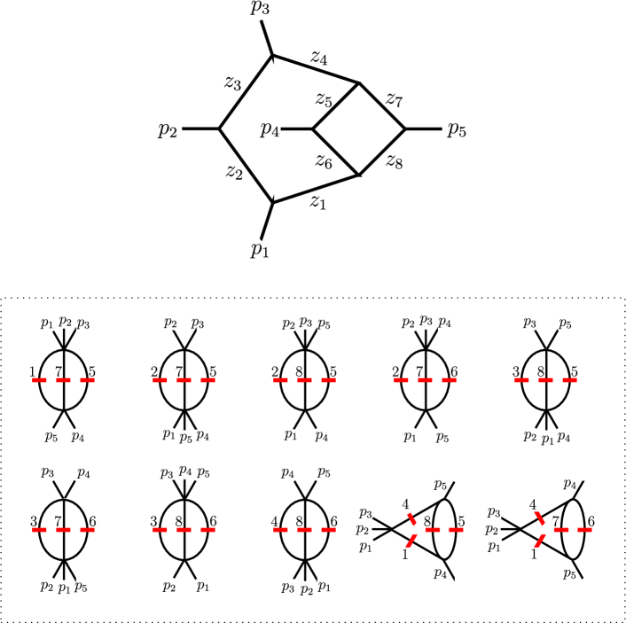
Figure 1: The fully massless non-planar hexagon-box diagram, along with our labelling conventions for its internal lines. The lower part shows the subset of the basis integrals with the property that their graphs cannot be obtained by adding internal lines to the graph of another basis integral. The corresponding cuts $\{1,5,7\}$, $\{2,5,7\}$, $\{2,5,8\}$, $\{2,6,7\}$, $\{3,5,8\}$, $\{3,6,7\}$, $\{3,6,8\}$, $\{4,6,8\}$, $\{1,4,5,8\}$ and $\{1,4,6,7\}$ are the cuts required for deriving complete IBP identities for the non-planar hexagon-box diagram.

We define the inverse propagators as follows, setting $P_{i\cdots j}\equiv p_{i}+\cdots+p_{j}$,

$$D_{1} =\ell_{1}^{2}\,,\hskip 22.76219pt D_{2}=(\ell_{1}-p_{1})^{2}\,,\hskip 22.76219pt D_{3}=(\ell_{1}-P_{12})^{2}\,,$$ (5.1)

$$D_{4} =(\ell_{1}-P_{123})^{2}\,,\hskip 22.76219pt D_{5}=(\ell_{1}+\ell_{2}+p_{4})^{2}\,,\hskip 22.76219pt D_{6}=(\ell_{1}+\ell_{2})^{2}\,,$$

$$D_{7} =(\ell_{2}-p_{5})^{2}\,,\hskip 22.76219pt D_{8}=\ell_{2}^{2}\,,\hskip 22.76219pt D_{9}=(\ell_{1}+p_{5})^{2}\,,$$

$$D_{10} =(\ell_{2}+p_{1})^{2}\,,\hskip 22.76219pt D_{11}=(\ell_{2}+p_{2})^{2}\,,\hskip 22.76219pt$$

and consider the family of Feynman integrals,

$$I(\nu_{1},\ldots,\nu_{11})=\int\frac{{\rm d}^{D}l_{1}}{i\pi^{D/2}}\frac{{\rm d}^{D}l_{2}}{i\pi^{D/2}}\frac{1}{D_{1}^{\nu_{1}}\cdots D_{11}^{\nu_{11}}}\,,$$ (5.2)

with $\nu_{9}\leq 0$, $\nu_{10}\leq 0$ and $\nu_{11}\leq 0$. In terms of the notation of subsection 2.1, we have $L=2$, $E=4$, $k=8$ and $m=11$. We furthermore define the Baikov variables $z_{i}\equiv D_{i}$, set $s_{ij}=(p_{i}+p_{j})^{2}$ and express the IBP identities in terms of the Mandelstam variables $s_{12},s_{13},s_{14},s_{23},s_{24}$. Using Azurite Georgoudis:2016wff we establish that, without applying global symmetries, there are $75$ “pre”-master integrals—i.e., master integrals where global symmetry relations have not yet been imposed. In the notation of eq. (5.2), they take the form,

$$\{{\mathcal{I}}_{1},\ldots,{\mathcal{I}}_{75}\}\equiv$$

$$\begin{array}[]{lll}\big{\{}I(1,1,1,1,1,1,1,1,-2,0,0),&I(1,1,1,1,1,1,1,1,-1,0,0),&I(1,1,1,1,1,1,1,1,0,0,0),\\ I(1,1,1,0,1,1,1,1,-1,0,0),&I(1,1,1,-1,1,1,1,1,0,0,0),&I(1,1,1,0,1,1,1,1,0,0,0),\\ I(1,1,-1,1,1,1,1,1,0,0,0),&I(1,1,0,1,1,1,1,1,0,0,0),&I(1,-1,1,1,1,1,1,1,0,0,0),\\ I(1,0,1,1,1,1,1,1,0,0,0),&I(0,1,1,1,1,1,1,1,-1,0,0),&I(-1,1,1,1,1,1,1,1,0,0,0),\\ I(0,1,1,1,1,1,1,1,0,0,0),&I(1,1,1,1,1,-1,0,1,0,0,0),&I(1,1,1,1,1,0,0,1,0,0,0),\\ I(1,1,1,1,-1,1,1,0,0,0,0),&I(1,1,1,1,0,1,1,0,0,0,0),&I(1,1,1,-1,1,1,1,0,0,0,0),\\ I(1,1,1,0,1,1,1,0,0,0,0),&I(1,1,1,-1,1,0,1,1,0,0,0),&I(1,1,1,0,1,0,1,1,0,0,0),\\ I(1,-1,1,0,1,1,1,1,0,0,0),&I(1,0,1,0,1,1,1,1,0,0,0),&I(1,0,0,1,1,1,1,1,0,0,0),\\ I(-1,1,1,1,1,1,0,1,0,0,0),&I(0,1,1,1,1,1,0,1,0,0,0),&I(-1,1,1,1,0,1,1,1,0,0,0),\\ I(0,1,1,1,0,1,1,1,0,0,0),&I(0,1,1,0,1,1,1,1,0,0,0),&I(-1,1,0,1,1,1,1,1,0,0,0),\\ I(0,1,0,1,1,1,1,1,0,0,0),&I(1,1,1,0,1,0,1,0,0,0,0),&I(1,1,1,0,1,0,0,1,0,0,0),\\ I(1,1,1,0,0,1,1,0,0,0,0),&I(1,1,0,1,1,0,0,1,0,0,0),&I(1,1,0,1,0,1,1,0,0,0,0),\\ I(1,1,0,0,1,1,1,0,0,0,0),&I(1,1,0,0,1,0,1,1,0,0,0),&I(1,0,1,1,1,0,0,1,0,0,0),\\ I(1,0,1,1,0,1,1,0,0,0,0),&I(1,-1,1,0,1,1,1,0,0,0,0),&I(1,0,1,0,1,1,1,0,0,0,0),\\ I(1,-1,1,0,1,0,1,1,0,0,0),&I(1,0,1,0,1,0,1,1,0,0,0),&I(0,1,1,1,1,0,0,1,0,0,0),\\ I(0,1,1,1,0,1,1,0,0,0,0),&I(0,1,1,1,0,1,0,1,0,0,0),&I(0,1,1,0,1,1,1,0,0,0,0),\\ I(0,1,1,0,1,1,0,1,0,0,0),&I(0,1,1,0,1,0,1,1,0,0,0),&I(0,1,1,0,0,1,1,1,0,0,0),\\ I(-1,1,0,1,1,1,0,1,0,0,0),&I(0,1,0,1,1,1,0,1,0,0,0),&I(-1,1,0,1,0,1,1,1,0,0,0),\\ I(0,1,0,1,0,1,1,1,0,0,0),&I(0,1,0,0,1,1,1,1,0,0,0),&I(0,0,1,1,1,1,0,1,0,0,0),\\ I(0,0,1,1,0,1,1,1,0,0,0),&I(0,0,1,0,1,1,1,1,0,0,0),&I(1,0,1,0,1,0,1,0,0,0,0),\\ I(1,0,1,0,1,0,0,1,0,0,0),&I(1,0,1,0,0,1,1,0,0,0,0),&I(1,0,0,1,1,0,0,1,0,0,0),\\ I(1,0,0,1,0,1,1,0,0,0,0),&I(0,1,0,1,1,0,0,1,0,0,0),&I(0,1,0,1,0,1,1,0,0,0,0),\\ I(0,1,0,1,0,1,0,1,0,0,0),&I(1,0,0,0,1,0,1,0,0,0,0),&I(0,1,0,0,1,0,1,0,0,0,0),\\ I(0,1,0,0,1,0,0,1,0,0,0),&I(0,1,0,0,0,1,1,0,0,0,0),&I(0,0,1,0,1,0,0,1,0,0,0),\\ I(0,0,1,0,0,1,1,0,0,0,0),&I(0,0,1,0,0,1,0,1,0,0,0),&I(0,0,0,1,0,1,0,1,0,0,0)\big{\}}\,.\end{array}$$ (5.28)

(5.29)

The graphs of these integrals are shown in figure 2. We remark that Azurite chooses master integrals which contain no doubled propagators.

Figure 2: (Color online.) The $75$ “pre”-master integrals found by Azurite, with the global symmetry option turned off, for the non-planar hexagon-box family of eq. (5.2). By turning on the global symmetry option, Azurite determines that there are $73$ master integrals. These are the illustrated “pre”-master integrals excluding $\mathcal{I}_{63}$ and $\mathcal{I}_{68}$. Our labeling convention for the propagators, corresponding to the indices recorded in eq. (5.29), are shown in the graph of the hexagon-box itself as the blue encircled numbers.

As explained at the end of section 2.2, the cuts that are necessary to construct the complete IBP identities are the maximal cuts of the “uncollapsible” master integrals in eq. (5.29). From this list of master integrals we find that the following $10$ cuts are necessary for computing the complete IBP identities,

$$\{1,5,7\},\{2,5,7\},\{2,5,8\},\{2,6,7\},\{3,5,8\},\{3,6,7\},\{3,6,8\},\{4,6,8\},$$

$$\{1,4,5,8\},\{1,4,6,7\}\,.$$ (5.30)

Here for example the notation $\{1,5,7\}$ means $\mathcal{S}_{\mathrm{cut}}=(\zeta_{1},\zeta_{2},\zeta_{3})=(1,5,7)$; that is, the triple cut,

$$z_{1}\to 0,\quad z_{5}\to 0,\quad z_{7}\to 0\,.$$ (5.31)

Thus, for the hexagon-box diagram, the set of necessary cuts thus includes $8$ triple cuts and $2$ quadruple cuts. The “pre”-master integrals supported on these cuts are listed in table 1.

The advantage of applying cuts is that the number of integrals in the IBP relations on each cut will be much less than when no cuts are applied.

cut	“pre”-master integrals
$\{1,5,7\}$	$\mathcal{I}_{1}$, $\mathcal{I}_{2}$, $\mathcal{I}_{3}$, $\mathcal{I}_{4}$, $\mathcal{I}_{5}$, $\mathcal{I}_{6}$, $\mathcal{I}_{7}$, $\mathcal{I}_{8}$, $\mathcal{I}_{9}$, $\mathcal{I}_{10}$, $\mathcal{I}_{18}$, $\mathcal{I}_{19}$, $\mathcal{I}_{20}$, $\mathcal{I}_{21}$, $\mathcal{I}_{22}$, $\mathcal{I}_{23}$, $\mathcal{I}_{24}$, $\mathcal{I}_{32}$, $\mathcal{I}_{37}$, $\mathcal{I}_{38}$, $\mathcal{I}_{41}$, $\mathcal{I}_{42}$, $\mathcal{I}_{43}$, $\mathcal{I}_{44}$, $\mathcal{I}_{60}$, $\mathcal{I}_{68}$
$\{2,5,7\}$	$\mathcal{I}_{1}$, $\mathcal{I}_{2}$, $\mathcal{I}_{3}$, $\mathcal{I}_{4}$, $\mathcal{I}_{5}$, $\mathcal{I}_{6}$, $\mathcal{I}_{7}$, $\mathcal{I}_{8}$, $\mathcal{I}_{11}$, $\mathcal{I}_{12}$, $\mathcal{I}_{13}$, $\mathcal{I}_{18}$, $\mathcal{I}_{19}$, $\mathcal{I}_{20}$, $\mathcal{I}_{21}$, $\mathcal{I}_{29}$, $\mathcal{I}_{30}$, $\mathcal{I}_{31}$, $\mathcal{I}_{32}$, $\mathcal{I}_{37}$, $\mathcal{I}_{38}$, $\mathcal{I}_{48}$, $\mathcal{I}_{50}$, $\mathcal{I}_{56}$, $\mathcal{I}_{69}$
$\{2,5,8\}$	$\mathcal{I}_{1}$, $\mathcal{I}_{2}$, $\mathcal{I}_{3}$, $\mathcal{I}_{4}$, $\mathcal{I}_{5}$, $\mathcal{I}_{6}$, $\mathcal{I}_{7}$, $\mathcal{I}_{8}$, $\mathcal{I}_{11}$, $\mathcal{I}_{12}$, $\mathcal{I}_{13}$, $\mathcal{I}_{14}$, $\mathcal{I}_{15}$, $\mathcal{I}_{20}$, $\mathcal{I}_{21}$, $\mathcal{I}_{25}$, $\mathcal{I}_{26}$, $\mathcal{I}_{29}$, $\mathcal{I}_{30}$, $\mathcal{I}_{31}$, $\mathcal{I}_{33}$, $\mathcal{I}_{35}$, $\mathcal{I}_{38}$, $\mathcal{I}_{45}$, $\mathcal{I}_{49}$, $\mathcal{I}_{50}$, $\mathcal{I}_{52}$, $\mathcal{I}_{53}$, $\mathcal{I}_{56}$, $\mathcal{I}_{65}$, $\mathcal{I}_{70}$
$\{2,6,7\}$	$\mathcal{I}_{1}$, $\mathcal{I}_{2}$, $\mathcal{I}_{3}$, $\mathcal{I}_{4}$, $\mathcal{I}_{5}$, $\mathcal{I}_{6}$, $\mathcal{I}_{7}$, $\mathcal{I}_{8}$, $\mathcal{I}_{11}$, $\mathcal{I}_{12}$, $\mathcal{I}_{13}$, $\mathcal{I}_{16}$, $\mathcal{I}_{17}$, $\mathcal{I}_{18}$, $\mathcal{I}_{19}$, $\mathcal{I}_{27}$, $\mathcal{I}_{28}$, $\mathcal{I}_{29}$, $\mathcal{I}_{30}$, $\mathcal{I}_{31}$, $\mathcal{I}_{34}$, $\mathcal{I}_{36}$, $\mathcal{I}_{37}$, $\mathcal{I}_{46}$, $\mathcal{I}_{48}$, $\mathcal{I}_{51}$, $\mathcal{I}_{54}$, $\mathcal{I}_{55}$, $\mathcal{I}_{56}$, $\mathcal{I}_{66}$, $\mathcal{I}_{71}$
$\{3,5,8\}$	$\mathcal{I}_{1}$, $\mathcal{I}_{2}$, $\mathcal{I}_{3}$, $\mathcal{I}_{4}$, $\mathcal{I}_{5}$, $\mathcal{I}_{6}$, $\mathcal{I}_{9}$, $\mathcal{I}_{10}$, $\mathcal{I}_{11}$, $\mathcal{I}_{12}$, $\mathcal{I}_{13}$, $\mathcal{I}_{14}$, $\mathcal{I}_{15}$, $\mathcal{I}_{20}$, $\mathcal{I}_{21}$, $\mathcal{I}_{22}$, $\mathcal{I}_{23}$, $\mathcal{I}_{25}$, $\mathcal{I}_{26}$, $\mathcal{I}_{29}$, $\mathcal{I}_{33}$, $\mathcal{I}_{39}$, $\mathcal{I}_{43}$, $\mathcal{I}_{44}$, $\mathcal{I}_{45}$, $\mathcal{I}_{49}$, $\mathcal{I}_{50}$, $\mathcal{I}_{57}$, $\mathcal{I}_{59}$, $\mathcal{I}_{61}$, $\mathcal{I}_{72}$
$\{3,6,7\}$	$\mathcal{I}_{1}$, $\mathcal{I}_{2}$, $\mathcal{I}_{3}$, $\mathcal{I}_{4}$, $\mathcal{I}_{5}$, $\mathcal{I}_{6}$, $\mathcal{I}_{9}$, $\mathcal{I}_{10}$, $\mathcal{I}_{11}$, $\mathcal{I}_{12}$, $\mathcal{I}_{13}$, $\mathcal{I}_{16}$, $\mathcal{I}_{17}$, $\mathcal{I}_{18}$, $\mathcal{I}_{19}$, $\mathcal{I}_{22}$, $\mathcal{I}_{23}$, $\mathcal{I}_{27}$, $\mathcal{I}_{28}$, $\mathcal{I}_{29}$, $\mathcal{I}_{34}$, $\mathcal{I}_{40}$, $\mathcal{I}_{41}$, $\mathcal{I}_{42}$, $\mathcal{I}_{46}$, $\mathcal{I}_{48}$, $\mathcal{I}_{51}$, $\mathcal{I}_{58}$, $\mathcal{I}_{59}$, $\mathcal{I}_{62}$, $\mathcal{I}_{73}$
$\{3,6,8\}$	$\mathcal{I}_{1}$, $\mathcal{I}_{2}$, $\mathcal{I}_{3}$, $\mathcal{I}_{4}$, $\mathcal{I}_{5}$, $\mathcal{I}_{6}$, $\mathcal{I}_{9}$, $\mathcal{I}_{10}$, $\mathcal{I}_{11}$, $\mathcal{I}_{12}$, $\mathcal{I}_{13}$, $\mathcal{I}_{22}$, $\mathcal{I}_{23}$, $\mathcal{I}_{25}$, $\mathcal{I}_{26}$, $\mathcal{I}_{27}$, $\mathcal{I}_{28}$, $\mathcal{I}_{29}$, $\mathcal{I}_{47}$, $\mathcal{I}_{49}$, $\mathcal{I}_{51}$, $\mathcal{I}_{57}$, $\mathcal{I}_{58}$, $\mathcal{I}_{59}$, $\mathcal{I}_{74}$
$\{4,6,8\}$	$\mathcal{I}_{1}$, $\mathcal{I}_{2}$, $\mathcal{I}_{3}$, $\mathcal{I}_{7}$, $\mathcal{I}_{8}$, $\mathcal{I}_{9}$, $\mathcal{I}_{10}$, $\mathcal{I}_{11}$, $\mathcal{I}_{12}$, $\mathcal{I}_{13}$, $\mathcal{I}_{24}$, $\mathcal{I}_{25}$, $\mathcal{I}_{26}$, $\mathcal{I}_{27}$, $\mathcal{I}_{28}$, $\mathcal{I}_{30}$, $\mathcal{I}_{31}$, $\mathcal{I}_{47}$, $\mathcal{I}_{52}$, $\mathcal{I}_{53}$, $\mathcal{I}_{54}$, $\mathcal{I}_{55}$, $\mathcal{I}_{57}$, $\mathcal{I}_{58}$, $\mathcal{I}_{67}$, $\mathcal{I}_{75}$
$\{1,4,5,8\}$	$\mathcal{I}_{1}$, $\mathcal{I}_{2}$, $\mathcal{I}_{3}$, $\mathcal{I}_{7}$, $\mathcal{I}_{8}$, $\mathcal{I}_{9}$, $\mathcal{I}_{10}$, $\mathcal{I}_{14}$, $\mathcal{I}_{15}$, $\mathcal{I}_{24}$, $\mathcal{I}_{35}$, $\mathcal{I}_{39}$, $\mathcal{I}_{63}$
$\{1,4,6,7\}$	$\mathcal{I}_{1}$, $\mathcal{I}_{2}$, $\mathcal{I}_{3}$, $\mathcal{I}_{7}$, $\mathcal{I}_{8}$, $\mathcal{I}_{9}$, $\mathcal{I}_{10}$, $\mathcal{I}_{16}$, $\mathcal{I}_{17}$, $\mathcal{I}_{24}$, $\mathcal{I}_{36}$, $\mathcal{I}_{40}$, $\mathcal{I}_{64}$

Table 1: “Pre”-master integrals supported on each of the $10$ cuts necessary to construct the complete IBP reductions.

If we switch on global symmetries in Azurite, then the number of independent master integrals is found to be $73$. This is due to the additional symmetry relations,

$$\mathcal{I}_{63}\equiv I(1,0,0,1,1,0,0,1,0,0,0) =I(1,0,0,1,0,1,1,0,0,0,0)\,,$$

$$\mathcal{I}_{68}\equiv I(1,0,0,0,1,0,1,0,0,0,0) =I(0,0,0,1,0,1,0,1,0,0,0)\,.$$ (5.32)

Hence the set of $73$ master integrals is,

$$\mathcal{F}_{\mathrm{MI}}=\{\mathcal{I}_{1},\ldots,\mathcal{I}_{75}\}\setminus\{\mathcal{I}_{63},\mathcal{I}_{68}\}\,.$$ (5.33)

In this paper, we first reduce integrals to the linear combination of $75$ “pre”-master integrals and then apply eq. (5.32) to further achieve the reduction to the linearly independent $73$ master integrals.

To demonstrate the power of our method, we show how to reduce all the numerator-degree-$4$, $3$, $2$ and $1$ hexagon-box integrals (our target integrals),

$$\begin{array}[]{lll}\{I(1,1,1,1,1,1,1,1,0,0,-4),&I(1,1,1,1,1,1,1,1,0,-1,-3),&I(1,1,1,1,1,1,1,1,0,-2,-2),\\ I(1,1,1,1,1,1,1,1,0,-3,-1),&I(1,1,1,1,1,1,1,1,0,-4,0),&I(1,1,1,1,1,1,1,1,-1,0,-3),\\ I(1,1,1,1,1,1,1,1,-1,-1,-2),&I(1,1,1,1,1,1,1,1,-1,-2,-1),&I(1,1,1,1,1,1,1,1,-1,-3,0),\\ I(1,1,1,1,1,1,1,1,-2,0,-2),&I(1,1,1,1,1,1,1,1,-2,-1,-1),&I(1,1,1,1,1,1,1,1,-2,-2,0),\\ I(1,1,1,1,1,1,1,1,-3,0,-1),&I(1,1,1,1,1,1,1,1,-3,-1,0),&I(1,1,1,1,1,1,1,1,-4,0,0),\\ I(1,1,1,1,1,1,1,1,0,0,-3),&I(1,1,1,1,1,1,1,1,0,-1,-2),&I(1,1,1,1,1,1,1,1,0,-2,-1),\\ I(1,1,1,1,1,1,1,1,0,-3,0),&I(1,1,1,1,1,1,1,1,-1,0,-2),&I(1,1,1,1,1,1,1,1,-1,-1,-1),\\ I(1,1,1,1,1,1,1,1,-1,-2,0),&I(1,1,1,1,1,1,1,1,-2,0,-1),&I(1,1,1,1,1,1,1,1,-2,-1,0),\\ I(1,1,1,1,1,1,1,1,-3,0,0),&I(1,1,1,1,1,1,1,1,0,0,-2),&I(1,1,1,1,1,1,1,1,0,-1,-1),\\ I(1,1,1,1,1,1,1,1,0,-2,0),&I(1,1,1,1,1,1,1,1,-1,0,-1),&I(1,1,1,1,1,1,1,1,-1,-1,0),\\ I(1,1,1,1,1,1,1,1,0,0,-1),&I(1,1,1,1,1,1,1,1,0,-1,0)\}\end{array}$$ (5.45)

(5.46)

analytically to express them as linear combinations of the $73$ master integrals.

5.1 Module intersection on cuts

In this section we show explicitly how to apply our module intersection method on cuts, in order to obtain simplified IBP systems (i.e., which do not involve integrals with doubled propagators) on unitarity cuts.

The module $M_{1}$ defined in subsection 2.1 for the hexagon-box diagram without cuts applied, is generated by the following $2\times(4+2)=12$ generators, cf. eq. (2.29),

$$(z_{1}-z_{2},z_{1}-z_{2},-s_{12}+z_{1}-z_{2},-s_{12}-s_{13}+z_{1}-z_{2},s_{14}+z_{1}-z_{2}-z_{8}+z_{10},z_{1}-z_{2}-z_{8}+z_{10},0,0,-s_{12}-s_{13}-s_{14}+z_{1}-z_{2},0,0)$$

$$(0,0,0,0,s_{14}+z_{1}-z_{2}-z_{8}+z_{10},z_{1}-z_{2}-z_{8}+z_{10},s_{12}+s_{13}+s_{14}-z_{8}+z_{10},z_{10}-z_{8},0,z_{10}-z_{8},s_{12}-z_{8}+z_{10})$$

$$(s_{12}+z_{2}-z_{3},z_{2}-z_{3},z_{2}-z_{3},-s_{23}+z_{2}-z_{3},s_{12}+s_{24}+z_{2}-z_{3}-z_{8}+z_{11},s_{12}+z_{2}-z_{3}-z_{8}+z_{11},0,0,-s_{23}-s_{24}+z_{2}-z_{3},0,0)$$

$$(0,0,0,0,s_{12}+s_{24}+z_{2}-z_{3}-z_{8}+z_{11},s_{12}+z_{2}-z_{3}-z_{8}+z_{11},s_{12}+s_{23}+s_{24}-z_{8}+z_{11},z_{11}-z_{8},0,s_{12}-z_{8}+z_{11},z_{11}-z_{8})$$

$$(s_{13}+s_{23}+z_{3}-z_{4},s_{23}+z_{3}-z_{4},z_{3}-z_{4},z_{3}-z_{4},-2s_{12}-s_{13}-s_{14}-s_{23}-s_{24}+z_{3}-z_{5}+z_{6}+z_{7}+z_{8}-z_{9}-z_{10}-z_{11},$$

$$-s_{12}+z_{3}-z_{5}+z_{6}+z_{7}+z_{8}-z_{9}-z_{10}-z_{11},0,0,s_{12}+s_{13}+s_{14}+s_{23}+s_{24}+z_{3}-z_{4},0,0)$$

$$(0,0,0,0,-2s_{12}-s_{13}-s_{14}-s_{23}-s_{24}+z_{3}-z_{5}+z_{6}+z_{7}+z_{8}-z_{9}-z_{10}-z_{11},-s_{12}+z_{3}-z_{5}+z_{6}+z_{7}+z_{8}-z_{9}-z_{10}-z_{11},$$

$$-2s_{12}-s_{13}-s_{14}-s_{23}-s_{24}+z_{4}-z_{5}+z_{6}+z_{7}+z_{8}-z_{9}-z_{10}-z_{11},-s_{12}-s_{13}-s_{23}+z_{4}-z_{5}+z_{6}+z_{7}+z_{8}-z_{9}-z_{10}-z_{11},$$

$$0,-s_{12}-s_{23}+z_{4}-z_{5}+z_{6}+z_{7}+z_{8}-z_{9}-z_{10}-z_{11},-s_{12}-s_{13}+z_{4}-z_{5}+z_{6}+z_{7}+z_{8}-z_{9}-z_{10}-z_{11})$$

$$(-s_{12}-s_{13}-s_{23}+z_{4}-z_{9},-s_{12}-s_{13}-s_{14}-s_{23}+z_{4}-z_{9},-s_{12}-s_{13}-s_{14}-s_{23}-s_{24}+z_{4}-z_{9},z_{4}-z_{9},z_{5}-z_{6},z_{5}-z_{6},0,0,z_{4}-z_{9},0,0)$$

$$(0,0,0,0,z_{5}-z_{6},z_{5}-z_{6},-z_{4}+z_{5}-z_{6}+z_{9},s_{12}+s_{13}+s_{23}-z_{4}+z_{5}-z_{6}+z_{9},$$

$$0,s_{12}+s_{13}+s_{14}+s_{23}-z_{4}+z_{5}-z_{6}+z_{9},s_{12}+s_{13}+s_{23}+s_{24}-z_{4}+z_{5}-z_{6}+z_{9})$$

$$(2z_{1},z_{1}+z_{2},-s_{12}+z_{1}+z_{3},-s_{12}-s_{13}-s_{23}+z_{1}+z_{4},-s_{12}-s_{13}-s_{23}+z_{1}+z_{4}+z_{6}-z_{8}-z_{9},z_{1}+z_{6}-z_{8},0,0,z_{1}+z_{9},0,0)$$

$$(0,0,0,0,-s_{12}-s_{13}-s_{23}+z_{1}+z_{4}+z_{6}-z_{8}-z_{9},z_{1}+z_{6}-z_{8},z_{6}-z_{8}-z_{9},-z_{1}+z_{6}-z_{8},0,-z_{2}+z_{6}-z_{8},s_{12}-z_{1}+z_{2}-z_{3}+z_{6}-z_{8})$$

$$(-z_{1}+z_{6}-z_{8},-z_{1}+z_{6}-z_{10},-z_{1}+z_{6}+z_{8}-z_{10}-z_{11},s_{12}+s_{13}+s_{23}-z_{1}-z_{4}+z_{5}-z_{7}+z_{9},$$

$$s_{12}+s_{13}+s_{23}-z_{1}-z_{4}+z_{5}+z_{8}+z_{9},-z_{1}+z_{6}+z_{8},0,0,-z_{1}+z_{6}-z_{7},0,0)$$

$$(0,0,0,0,s_{12}+s_{13}+s_{23}-z_{1}-z_{4}+z_{5}+z_{8}+z_{9},-z_{1}+z_{6}+z_{8},z_{7}+z_{8},2z_{8},0,z_{8}+z_{10},z_{8}+z_{11})\,.$$ (5.47)

Note that the generators are at most linear in the $z_{i}$, and always homogeneous in $z_{1},\ldots,z_{11}$ and $s_{12},s_{13},s_{14},s_{23},s_{24}$.

The module $M_{2}$ for the hexagon-box diagram without applied cuts is generated by the following $11$ generators, cf. eq. (2.30),

$$(z_{1},0,0,0,0,0,0,0,0,0,0),(0,z_{2},0,0,0,0,0,0,0,0,0)$$

$$(0,0,z_{3},0,0,0,0,0,0,0,0),(0,0,0,z_{4},0,0,0,0,0,0,0)$$

$$(0,0,0,0,z_{5},0,0,0,0,0,0),(0,0,0,0,0,z_{6},0,0,0,0,0)$$

$$(0,0,0,0,0,0,z_{7},0,0,0,0),(0,0,0,0,0,0,0,z_{8},0,0,0)$$

$$(0,0,0,0,0,0,0,0,1,0,0),(0,0,0,0,0,0,0,0,0,1,0)$$

$$(0,0,0,0,0,0,0,0,0,0,1)\,.$$ (5.48)

We now proceed to consider the modules on the unitarity cuts given in eq. (5.30). For example, for the cut $\{2,5,7\}$, we apply the replacements

$$z_{2}\to 0\,,\quad z_{5}\to 0\,,\quad z_{7}\to 0\,.$$ (5.49)

The propagator indices are thus classified as,

$$\mathcal{S}_{\mathrm{cut}}=\{2,5,7\}\,,\quad\mathcal{S}_{\mathrm{uncut}}=\{1,3,4,6,8\}\,,\quad\mathcal{S}_{\mathrm{ISP}}=\{9,10,11\}\,.$$ (5.50)

From eq. (2.23) it follows that the generators of $\tilde{M}_{1}$ on the cut $\{2,5,7\}$ take the form,

$$(z_{1},z_{1},z_{1}-s_{12},-s_{12}-s_{13}+z_{1},s_{14}+z_{1}-z_{8}+z_{10},z_{1}-z_{8}+z_{10},0,0,-s_{12}-s_{13}-s_{14}+z_{1},0,0)$$

$$(0,0,0,0,s_{14}+z_{1}-z_{8}+z_{10},z_{1}-z_{8}+z_{10},s_{12}+s_{13}+s_{14}-z_{8}+z_{10},z_{10}-z_{8},0,z_{10}-z_{8},s_{12}-z_{8}+z_{10})$$

$$(s_{12}-z_{3},-z_{3},-z_{3},-s_{23}-z_{3},s_{12}+s_{24}-z_{3}-z_{8}+z_{11},s_{12}-z_{3}-z_{8}+z_{11},0,0,-s_{23}-s_{24}-z_{3},0,0)$$

$$(0,0,0,0,s_{12}+s_{24}-z_{3}-z_{8}+z_{11},s_{12}-z_{3}-z_{8}+z_{11},s_{12}+s_{23}+s_{24}-z_{8}+z_{11},z_{11}-z_{8},0,s_{12}-z_{8}+z_{11},z_{11}-z_{8})$$

$$(s_{13}+s_{23}+z_{3}-z_{4},s_{23}+z_{3}-z_{4},z_{3}-z_{4},z_{3}-z_{4},-2s_{12}-s_{13}-s_{14}-s_{23}-s_{24}+z_{3}+z_{6}+z_{8}-z_{9}-z_{10}-z_{11},$$

$$-s_{12}+z_{3}+z_{6}+z_{8}-z_{9}-z_{10}-z_{11},0,0,s_{12}+s_{13}+s_{14}+s_{23}+s_{24}+z_{3}-z_{4},0,0)$$

$$(0,0,0,0,-2s_{12}-s_{13}-s_{14}-s_{23}-s_{24}+z_{3}+z_{6}+z_{8}-z_{9}-z_{10}-z_{11},-s_{12}+z_{3}+z_{6}+z_{8}-z_{9}-z_{10}-z_{11},$$

$$-2s_{12}-s_{13}-s_{14}-s_{23}-s_{24}+z_{4}+z_{6}+z_{8}-z_{9}-z_{10}-z_{11},-s_{12}-s_{13}-s_{23}+z_{4}+z_{6}+z_{8}-z_{9}-z_{10}-z_{11},$$

$$0,-s_{12}-s_{23}+z_{4}+z_{6}+z_{8}-z_{9}-z_{10}-z_{11},-s_{12}-s_{13}+z_{4}+z_{6}+z_{8}-z_{9}-z_{10}-z_{11})$$

$$(-s_{12}-s_{13}-s_{23}+z_{4}-z_{9},-s_{12}-s_{13}-s_{14}-s_{23}+z_{4}-z_{9},-s_{12}-s_{13}-s_{14}-s_{23}-s_{24}+z_{4}-z_{9},z_{4}-z_{9},-z_{6},-z_{6},0,0,z_{4}-z_{9},0,0)$$

$$(0,0,0,0,-z_{6},-z_{6},-z_{4}-z_{6}+z_{9},s_{12}+s_{13}+s_{23}-z_{4}-z_{6}+z_{9},0,s_{12}+s_{13}+s_{14}+s_{23}-z_{4}-z_{6}+z_{9},s_{12}+s_{13}+s_{23}+s_{24}-z_{4}-z_{6}+z_{9})$$

$$(2z_{1},z_{1},-s_{12}+z_{1}+z_{3},-s_{12}-s_{13}-s_{23}+z_{1}+z_{4},-s_{12}-s_{13}-s_{23}+z_{1}+z_{4}+z_{6}-z_{8}-z_{9},z_{1}+z_{6}-z_{8},0,0,z_{1}+z_{9},0,0)$$

$$(0,0,0,0,-s_{12}-s_{13}-s_{23}+z_{1}+z_{4}+z_{6}-z_{8}-z_{9},z_{1}+z_{6}-z_{8},z_{6}-z_{8}-z_{9},-z_{1}+z_{6}-z_{8},0,z_{6}-z_{8},s_{12}-z_{1}-z_{3}+z_{6}-z_{8})$$

$$(-z_{1}+z_{6}-z_{8},-z_{1}+z_{6}-z_{10},-z_{1}+z_{6}+z_{8}-z_{10}-z_{11},s_{12}+s_{13}+s_{23}-z_{1}-z_{4}+z_{9},s_{12}+s_{13}+s_{23}-z_{1}-z_{4}+z_{8}+z_{9},$$

$$-z_{1}+z_{6}+z_{8},0,0,z_{6}-z_{1},0,0)$$

$$(0,0,0,0,s_{12}+s_{13}+s_{23}-z_{1}-z_{4}+z_{8}+z_{9},-z_{1}+z_{6}+z_{8},z_{8},2z_{8},0,z_{8}+z_{10},z_{8}+z_{11})\,,$$ (5.51)

whereas the generators of $\tilde{M}_{2}$ on the cut $\{2,5,7\}$ take the form,

$$(z_{1},0,0,0,0,0,0,0,0,0,0),(0,0,z_{3},0,0,0,0,0,0,0,0)$$

$$(0,0,0,z_{4},0,0,0,0,0,0,0),(0,0,0,0,0,z_{6},0,0,0,0,0)$$

$$(0,0,0,0,0,0,0,z_{8},0,0,0),(0,0,0,0,0,0,0,0,1,0,0)$$

$$(0,0,0,0,0,0,0,0,0,1,0),(0,0,0,0,0,0,0,0,0,0,1)\,.$$ (5.52)

The intersection of $\tilde{M}_{1}$ and $\tilde{M}_{2}$, with the generators given above, is then computed by the method described in section 3. In the case at hand, we proceed as follows.

1. First we compute the generators $\tilde{M}_{1}\cap\tilde{M}_{2}$ in the ring, with the algorithm described in Lemma 3,

   $$\mathbb{B}=\mathbb{Q}[z_{1},z_{3},z_{4},z_{6},z_{8},z_{9},z_{10},z_{11},s_{12},s_{13},s_{14},s_{23},s_{24}]$$ (5.53)

   using a block ordering with $[z_{1},z_{3},z_{4},z_{6},z_{8},z_{9},z_{10},z_{11}]\succ[s_{12},s_{13},s_{14},s_{23},s_{24}]$.

2. Then we map the generators of $\tilde{M}_{1}\cap\tilde{M}_{2}$ from the previous step, to the ring,

   $$\tilde{\mathbb{A}}=\mathbb{Q}(s_{12},s_{13},s_{14},s_{23},s_{24})[z_{1},z_{3},z_{4},z_{6},z_{8},z_{9},z_{10},z_{11}]$$ (5.54)

   and simplify the generators.

3. Finally, we use the heuristic algorithm (Algorithm 8) to delete redundant generators in $\tilde{M}_{1}\cap\tilde{M}_{2}$.

These steps are automated by our Singular program. The generators of $\tilde{M}_{1}\cap\tilde{M}_{2}$ for the other $9$ cuts listed in eq. (5.30) were obtained in the same manner. In table 2 we provide timings for the computation of the module intersections for the relevant cuts of the non-planar hexagon-box diagram. The timings are in seconds on an Intel Xeon E5-2643 machine with $24$ cores, $3.40$ GHz and $384$ GB of RAM.

cut	time / sec	mem/GB
$\{1,5,7\}$	$218$	4.3
$\{2,5,7\}$	$43$	1.1
$\{2,5,8\}$	$303$	6.7
$\{2,6,7\}$	$743$	9.8
$\{3,5,8\}$	$404$	7.4
$\{3,6,7\}$	$699$	11.0
$\{3,6,8\}$	$24$	1.0
$\{4,6,8\}$	$797$	13.7
$\{1,4,5,8\}$	$53$	1.7
$\{1,4,6,7\}$	$196$	3.0

Table 2: Timings and RAM usages for the module intersection computations for the relevant cuts of the non-planar hexagon-box diagram.

Furthermore, using the heuristics as specified in Algorithm 8 we are able to reduce the size of the generating systems as specified in table 3. For instance, the trimmed generating system for the module intersection on the cut $\{2,5,7\}$ consists of $24$ generators, which are fully analytic in $s_{12},s_{13},s_{14},s_{23},s_{24}$. The generators can be downloaded from

https://raw.githubusercontent.com/yzhphy/hexagonbox_reduction/master/cut257/module_intersection_257.txt .

Each list in this file is in the format

$$(\tilde{b}_{1},0,\tilde{b}_{3},\tilde{b}_{4},0,\tilde{b}_{6},0,\tilde{b}_{8},\tilde{a}_{9},\tilde{a}_{10},\tilde{a}_{11},\tilde{b})\,.$$ (5.55)

cut	original size / MB	trimmed size / MB
$\{1,5,7\}$	$68$	$10$
$\{2,5,7\}$	$25$	$1.4$
$\{2,5,8\}$	$49$	$3.1$
$\{2,6,7\}$	$100$	$2.8$
$\{3,5,8\}$	$97$	$3.7$
$\{3,6,7\}$	$80$	$3.6$
$\{3,6,8\}$	$10$	$1.6$
$\{4,6,8\}$	$21$	$1.6$
$\{1,4,5,8\}$	$4.4$	$3.6$
$\{1,4,6,7\}$	$9.4$	$4.1$

Table 3: String sizes of the original and trimmed generating systems, given in megabytes.

5.2 Reduction of IBP identities on cuts

After computing the module intersections on the $10$ cuts, we use eq. (2.26) to generate IBP identities without doubled propagators on each cut in turn. As described in section 4, we use linear algebra techniques to select the relevant and independent IBP identities for reducing the target integrals to the master integrals on each cut. Characteristics of the resulting linearly independent linear systems, all analytic in $s_{12},s_{13},s_{14},s_{23},s_{24}$ and the spacetime dimension $D$, are presented in table 4.

cut	# equations	# integrals	byte size / MB	density
$\{1,5,7\}$	$1144$	$1177$	$1.2$	$1.4\%$
$\{2,5,7\}$	$1170$	$1210$	$0.99$	$1.3\%$
$\{2,5,8\}$	$1152$	$1190$	$1.1$	$1.5\%$
$\{2,6,7\}$	$1118$	$1155$	$1.0$	$1.5\%$
$\{3,5,8\}$	$1160$	$1202$	$1.2$	$1.5\%$
$\{3,6,7\}$	$1173$	$1217$	$1.3$	$1.7\%$
$\{3,6,8\}$	$1135$	$1176$	$0.77$	$1.2\%$
$\{4,6,8\}$	$1140$	$1176$	$0.94$	$1.2\%$
$\{1,4,5,8\}$	$700$	$723$	$0.69$	$1.7\%$
$\{1,4,6,7\}$	$683$	$706$	$0.66$	$1.6\%$

Table 4: Linear systems of IBP identities on the $10$ cuts given in eq. (5.30) for reducing the target hexagon-box integrals in eq. (5.46). The storage size is for the corresponding matrix and is measured in megabytes. The density refers to the percentage of non-vanishing elements in the matrices of these linear systems.

It is clear from this table that these linear systems are very sparse and of relatively small byte size.

For the purpose of demonstration, we have made the IBP relations on the cut $\{2,5,7\}$ available at

https://raw.githubusercontent.com/yzhphy/hexagonbox_reduction/master/cut257/hexagonbox_257_deg4.txt   .

We calculated the row reduced echelon form (RREF) of these linear systems using the total pivoting strategy, in order to retain the sparsity in intermediate steps. For the linear systems corresponding to some cuts, we are able to directly obtain the RREF analytically in $s_{12},s_{13},s_{14},s_{23},s_{24}$ and the spacetime dimension $D$. For linear systems corresponding to other cuts, we calculate the RREF with integer values of one or two $s_{ij}$ repeatedly. The fully analytic RREF is then readily obtained by our private heuristic interpolation algorithm. These computations are implemented in our primitive Mathematica code. A much more efficient RREF code in Singular is in preparation.

We also remark that for the computation of different cuts, a useful trick is to work with different choices of independent Mandelstam invariants. For a specific cut, a suitable choice of Mandelstam invariants can speed up the computation and also save the RAM usage. After the RREF is obtained, we use the program Fermat Fermat to replace the new Mandelstam variables by the original choice $s_{12},s_{13},s_{14},s_{23},s_{24}$.

The running time and resources required of our Mathematica code depends on the size of the linear systems and also the complexity of coefficients in the reduced IBPs. For the smallest linear system, the one corresponding to the quadruple cut $\{1,4,6,7\}$, our Mathematica RREF code obtained the fully analytical RREF in $31$ minutes with one core and $1.5$ GB RAM usage on a laptop with $16$ GB RAM. For the largest linear system, that corresponding to the triple cut $\{3,6,7\}$, we run our Mathematica code and assign integer values to two Mandelstam invariants. This finished in $2.5$ hours and used $1.8$ GB RAM. We parallelize the running with various integer values, evaluating $440$ points on the IRIDIS High Performance Computing Facility. The semi-analytic results are then interpolated to the fully analytic RREF result by our heuristic multivariate interpolation algorithm, requiring a CPU time of $23$ minutes with one core and $15$ GB RAM usage.

5.3 Merging of IBP reductions and final result

Having obtained the RREF of the $10$ IBP systems on cuts, it is straightforward to merge the coefficients to obtain the complete IBP reductions without applied cuts Larsen:2015ped . For example, to determine the reduction coefficient of $\mathcal{I}_{42}=I(1,0,1,0,1,1,1,0,0,0,0)$, we search for $\mathcal{I}_{42}$ in table 1 and find that it is supported on the cuts $\{1,5,7\}$ and $\{3,6,7\}$. We find that, for every target integral, the reduction coefficient for $\mathcal{I}_{42}$ on the cut $\{1,5,7\}$ equals the corresponding coefficient on the cut $\{3,6,7\}$, as must be the case. Thus, for each target integral in turn, we obtain its reduction coefficient of each $\mathcal{I}_{j}$ as the reduction coefficient of $\mathcal{I}_{j}$ on each cut supporting $\mathcal{I}_{j}$. In this way we obtain the complete reduction of the target integral without applied cuts.

After merging the $10$ RREFs we reduce the $32$ target integrals in eq. (5.46) to the $75$ “pre”-master integrals $\{\mathcal{I}_{1},\ldots,\mathcal{I}_{75}\}$. We then apply the global symmetry in eq. (5.32) to eliminate the redundant integrals $\mathcal{I}_{63}$ and $\mathcal{I}_{68}$, and then finally obtain the complete analytic reduction to the $73$ master integrals. The IBP reduction result, as replacement rules (in a compressed file of the size $280$ MB), can be downloaded from the link provided in the introduction.

5.4 Comparison with other IBP solvers

We have checked our results with FIRE5 Smirnov:2014hma in the C++ implementation with LiteRed Lee:2012cn , and KIRA (v 1.1) Maierhoefer:2017hyi . We note that it is not an easy task to perform the analytic IBP reduction of hexagon-box integrals with degree-four numerators. Due to the RAM limit we faced, we have not yet been able to obtain the analytic IBP reduction for degree-four-numerator hexagon-box integrals from FIRE5 or KIRA with the Rackham cluster, on a node with two $10$ core Intel Xeon V4 CPU and $256$ GB of RAM. On the other hand, it is easy to obtain the numeric IBP reduction for degree-four-numerator hexagon-box integrals with FIRE5 and KIRA. For example, if all the five $s_{ij}$ are taken to be integers, FIRE5 is able to generate the purely numeric IBP reductions in about $6.0$ hours. We ran FIRE5 purely numerically for many sets of integer values, and all the numeric IBP reduction results are consistent with our analytic IBP reductions, after a basis change between the Azurite integral basis and the FIRE basis.

6 Conclusion and outlook

In this paper we have presented a new and efficient method for computing integration-by-parts (IBP) reductions based on the ideas developed in refs. Larsen:2015ped ; Zhang:2016kfo . We used a module intersection method Zhang:2016kfo to trim IBP systems on unitarity cuts. The key idea is the efficient analytic computation of module intersections, which is achieved by the mathematical technique of treating the kinematical parameters as variables and using a block monomial ordering for which [variables] $\succ$ [parameters]. This trick could also be helpful for other types of multi-loop multi-scale amplitude computations. After solving the module intersection problems, we find linear IBP systems on cuts which are of very small sizes. This part is implemented in our highly efficient and automated Singular code. For example, the analytic IBP vectors for the hexagon-box integral with no doubled propagators on triple cuts can be computed in minutes.

Furthermore, we applied sophisticated sparse linear algebra techniques to compute the row reduced echelon form of the IBP identities on cuts. For example, we applied a weighted version of the Markowitz pivoting strategy to retain the sparsity in intermediate steps of the row reduction. We have implemented the sparse linear algebra part of our algorithm as a preliminary Mathematica code. A more efficient Singular implementation will become available in the near future.

In this paper, we have solved a cutting-edge IBP reduction problem fully analytically: that of the reduction of non-planar five-point hexagon-box integrals, with numerators of degree four, to the basis of $73$ master integrals. Our result has been verified (numerically) with the state-of-art IBP reduction programs.

We are currently preparing an automated implementation based on open-source software, such as Singular, with which we expect to be able to solve yet more difficult IBP reduction problems. We expect that our method will boost the computation of NNLO cross sections for more complicated $2\rightarrow 3$ scattering processes and higher-multiplicity cases.

Finally, we also expect that the ideas presented in this paper, such as the module intersection for trimming integral relations, the special ordering for variables and parameters, and sparse linear algebra techniques, can also be combined in various ways with other existing computational methods such as: the finite field sampling and reconstruction approach vonManteuffel:2014ixa ; Peraro:2016wsq , the dual conformal symmetry construction of IBP vectors Bern:2017gdk and the newly developed D-module method Bitoun:2017nre , in order to determine tailored optimal reduction strategies for various classes of Feynman integrals.

References

• (1) S. Laporta, Calculation of master integrals by difference equations, Phys. Lett. B504 (2001) 188–194, [hep-ph/0102032].
• (2) S. Laporta, High precision calculation of multiloop Feynman integrals by difference equations, Int. J. Mod. Phys. A15 (2000) 5087–5159, [hep-ph/0102033].
• (3) C. Anastasiou and A. Lazopoulos, Automatic integral reduction for higher order perturbative calculations, JHEP 07 (2004) 046, [hep-ph/0404258].
• (4) A. V. Smirnov, Algorithm FIRE – Feynman Integral REduction, JHEP 10 (2008) 107, [arXiv:0807.3243].
• (5) A. V. Smirnov, FIRE5: a C++ implementation of Feynman Integral REduction, Comput. Phys. Commun. 189 (2014) 182–191, [arXiv:1408.2372].
• (6) C. Studerus, Reduze-Feynman Integral Reduction in C++, Comput. Phys. Commun. 181 (2010) 1293–1300, [arXiv:0912.2546].
• (7) A. von Manteuffel and C. Studerus, Reduze 2 - Distributed Feynman Integral Reduction, arXiv:1201.4330.
• (8) R. N. Lee, Presenting LiteRed: a tool for the Loop InTEgrals REDuction, arXiv:1212.2685.
• (9) P. Maierhoefer, J. Usovitsch, and P. Uwer, Kira - A Feynman Integral Reduction Program, Comput. Phys. Commun. 230 (2018) 99–112, [arXiv:1705.05610].
• (10) J. Gluza, K. Kajda, and D. A. Kosower, Towards a Basis for Planar Two-Loop Integrals, Phys.Rev. D83 (2011) 045012, [arXiv:1009.0472].
• (11) R. M. Schabinger, A New Algorithm For The Generation Of Unitarity-Compatible Integration By Parts Relations, JHEP 01 (2012) 077, [arXiv:1111.4220].
• (12) H. Ita, Two-loop Integrand Decomposition into Master Integrals and Surface Terms, Phys. Rev. D94 (2016), no. 11 116015, [arXiv:1510.05626].
• (13) K. J. Larsen and Y. Zhang, Integration-by-parts reductions from unitarity cuts and algebraic geometry, Phys. Rev. D93 (2016), no. 4 041701, [arXiv:1511.01071].
• (14) A. von Manteuffel and R. M. Schabinger, A novel approach to integration by parts reduction, Phys. Lett. B744 (2015) 101–104, [arXiv:1406.4513].
• (15) Z. Bern, M. Enciso, H. Ita, and M. Zeng, Dual Conformal Symmetry, Integration-by-Parts Reduction, Differential Equations and the Nonplanar Sector, Phys. Rev. D96 (2017), no. 9 096017, [arXiv:1709.06055].
• (16) D. A. Kosower, Direct Solution of Integration-by-Parts Systems, arXiv:1804.00131.
• (17) R. N. Lee and A. A. Pomeransky, Critical points and number of master integrals, JHEP 11 (2013) 165, [arXiv:1308.6676].
• (18) A. Georgoudis, K. J. Larsen, and Y. Zhang, Azurite: An algebraic geometry based package for finding bases of loop integrals, Comput. Phys. Commun. 221 (2017) 203–215, [arXiv:1612.04252].
• (19) T. Bitoun, C. Bogner, R. P. Klausen, and E. Panzer, Feynman integral relations from parametric annihilators, arXiv:1712.09215.
• (20) R. Britto, F. Cachazo, and B. Feng, Generalized unitarity and one-loop amplitudes in N=4 super-Yang-Mills, Nucl. Phys. B725 (2005) 275–305, [hep-th/0412103].
• (21) R. Britto, F. Cachazo, B. Feng, and E. Witten, Direct proof of tree-level recursion relation in Yang-Mills theory, Phys. Rev. Lett. 94 (2005) 181602, [hep-th/0501052].
• (22) D. A. Kosower and K. J. Larsen, Maximal Unitarity at Two Loops, Phys. Rev. D85 (2012) 045017, [arXiv:1108.1180].
• (23) H. Johansson, D. A. Kosower, and K. J. Larsen, Two-Loop Maximal Unitarity with External Masses, Phys. Rev. D87 (2013), no. 2 025030, [arXiv:1208.1754].
• (24) G. Ossola, C. G. Papadopoulos, and R. Pittau, Reducing full one-loop amplitudes to scalar integrals at the integrand level, Nucl. Phys. B763 (2007) 147–169, [hep-ph/0609007].
• (25) S. Badger, H. Frellesvig, and Y. Zhang, Hepta-Cuts of Two-Loop Scattering Amplitudes, JHEP 04 (2012) 055, [arXiv:1202.2019].
• (26) Y. Zhang, Integrand-Level Reduction of Loop Amplitudes by Computational Algebraic Geometry Methods, JHEP 09 (2012) 042, [arXiv:1205.5707].
• (27) P. Mastrolia, E. Mirabella, G. Ossola, and T. Peraro, Scattering Amplitudes from Multivariate Polynomial Division, Phys. Lett. B718 (2012) 173–177, [arXiv:1205.7087].
• (28) A. V. Kotikov, Differential equations method: New technique for massive Feynman diagrams calculation, Phys. Lett. B254 (1991) 158–164.
• (29) A. V. Kotikov, Differential equation method: The Calculation of N point Feynman diagrams, Phys. Lett. B267 (1991) 123–127.
• (30) Z. Bern, L. J. Dixon, and D. A. Kosower, Dimensionally regulated pentagon integrals, Nucl. Phys. B412 (1994) 751–816, [hep-ph/9306240].
• (31) E. Remiddi, Differential equations for Feynman graph amplitudes, Nuovo Cim. A110 (1997) 1435–1452, [hep-th/9711188].
• (32) T. Gehrmann and E. Remiddi, Differential equations for two loop four point functions, Nucl. Phys. B580 (2000) 485–518, [hep-ph/9912329].
• (33) J. M. Henn, Multiloop integrals in dimensional regularization made simple, Phys. Rev. Lett. 110 (2013) 251601, [arXiv:1304.1806].
• (34) C. G. Papadopoulos, Simplified differential equations approach for Master Integrals, JHEP 07 (2014) 088, [arXiv:1401.6057].
• (35) R. N. Lee, Reducing differential equations for multiloop master integrals, JHEP 04 (2015) 108, [arXiv:1411.0911].
• (36) J. Ablinger, A. Behring, J. Blümlein, A. De Freitas, A. von Manteuffel, and C. Schneider, Calculating Three Loop Ladder and V-Topologies for Massive Operator Matrix Elements by Computer Algebra, Comput. Phys. Commun. 202 (2016) 33–112, [arXiv:1509.08324].
• (37) C. G. Papadopoulos, D. Tommasini, and C. Wever, The Pentabox Master Integrals with the Simplified Differential Equations approach, JHEP 04 (2016) 078, [arXiv:1511.09404].
• (38) X. Liu, Y.-Q. Ma, and C.-Y. Wang, A Systematic and Efficient Method to Compute Multi-loop Master Integrals, Phys. Lett. B779 (2018) 353–357, [arXiv:1711.09572].
• (39) S. Badger, H. Frellesvig, and Y. Zhang, A Two-Loop Five-Gluon Helicity Amplitude in QCD, JHEP 12 (2013) 045, [arXiv:1310.1051].
• (40) S. Badger, G. Mogull, A. Ochirov, and D. O’Connell, A Complete Two-Loop, Five-Gluon Helicity Amplitude in Yang-Mills Theory, JHEP 10 (2015) 064, [arXiv:1507.08797].
• (41) T. Gehrmann, J. M. Henn, and N. A. Lo Presti, Analytic form of the two-loop planar five-gluon all-plus-helicity amplitude in QCD, Phys. Rev. Lett. 116 (2016), no. 6 062001, [arXiv:1511.05409]. [Erratum: Phys. Rev. Lett.116,no.18,189903(2016)].
• (42) S. Badger, C. Brønnum-Hansen, H. B. Hartanto, and T. Peraro, First look at two-loop five-gluon scattering in QCD, Phys. Rev. Lett. 120 (2018), no. 9 092001, [arXiv:1712.02229].
• (43) S. Abreu, F. Febres Cordero, H. Ita, B. Page, and M. Zeng, Planar Two-Loop Five-Gluon Amplitudes from Numerical Unitarity, arXiv:1712.03946.
• (44) R. H. Boels, Q. Jin, and H. Luo, Efficient integrand reduction for particles with spin, arXiv:1802.06761.
• (45) O. V. Tarasov, Connection between Feynman integrals having different values of the space-time dimension, Phys. Rev. D54 (1996) 6479–6490, [hep-th/9606018].
• (46) R. N. Lee, Space-time dimensionality D as complex variable: Calculating loop integrals using dimensional recurrence relation and analytical properties with respect to D, Nucl. Phys. B830 (2010) 474–492, [arXiv:0911.0252].
• (47) R. N. Lee, Calculating multiloop integrals using dimensional recurrence relation and $D$-analyticity, Nucl. Phys. Proc. Suppl. 205-206 (2010) 135–140, [arXiv:1007.2256].
• (48) Y. Zhang, Lecture Notes on Multi-loop Integral Reduction and Applied Algebraic Geometry, 2016. arXiv:1612.02249.
• (49) P. Gianni, B. Trager, and G. Zacharias, Groebner bases and primary decomposition of polynomial ideals, Journal of Symbolic Computation 6 (1988), no. 2 149 – 167.
• (50) W. Decker, G.-M. Greuel, G. Pfister, and H. Schönemann, “Singular 4-1-1 — A computer algebra system for polynomial computations.” http://www.singular.uni-kl.de, 2018.
• (51) P. A. Baikov, Explicit solutions of the three loop vacuum integral recurrence relations, Phys. Lett. B385 (1996) 404–410, [hep-ph/9603267].
• (52) R. N. Lee, Modern techniques of multiloop calculations, in Proceedings, 49th Rencontres de Moriond on QCD and High Energy Interactions: La Thuile, Italy, March 22-29, 2014, pp. 297–300, 2014. arXiv:1405.5616.
• (53) H. Hauser and G. Müller, Affine varieties and lie algebras of vector fields, manuscripta mathematica 80 (1993), no. 1 309–337.
• (54) J. Boehm, A. Georgoudis, K. J. Larsen, M. Schulze, and Y. Zhang, Complete sets of logarithmic vector fields for integration-by-parts identities of Feynman integrals, arXiv:1712.09737.
• (55) R. N. Lee and A. A. Pomeransky, Normalized Fuchsian form on Riemann sphere and differential equations for multiloop integrals, arXiv:1707.07856.
• (56) D. Eisenbud, Commutative algebra - With a view toward algebraic geometry, vol. 150 of Graduate Texts in Mathematics. Springer-Verlag, New York, 1995.
• (57) T. Józefiak, Ideals generated by minors of a symmetric matrix, Comment. Math. Helv. 53 (1978), no. 4 595–607.
• (58) G.-M. Greuel and G. Pfister, A Singular Introduction to Commutative Algebra. Springer Publishing Company, Incorporated, 2nd ed., 2007.
• (59) J. Boehm, W. Decker, C. Fieker, and G. Pfister, The use of Bad Primes in Rational Reconstruction, Math. Comp. 84 (2015) 3013, [arXiv:1207.1651].
• (60) J. Boehm, W. Decker, C. Fieker, S. Laplagne, and G. Pfister, Bad Primes in Computational Algebraic Geometry, LNCS 9725 (2016) 93, [arXiv:1702.06920].
• (61) The_SpaSM_group, SpaSM: a Sparse direct Solver Modulo $p$, v1.2 ed., 2017. http://github.com/cbouilla/spasm.
• (62) H. M. Markowitz, The elimination form of the inverse and its application to linear programming, Management Science 3 (1957), no. 3 255–269, [https://doi.org/10.1287/mnsc.3.3.255].
• (63) D. Chicherin, J. Henn, and V. Mitev, Bootstrapping pentagon functions, JHEP 05 (2018) 164, [arXiv:1712.09610].
• (64) D. Chicherin, J. M. Henn, and E. Sokatchev, Amplitudes from superconformal Ward identities, arXiv:1804.03571.
• (65) R. H. Lewis, Computer Algebra System Fermat, v6.1.9 ed., 2018. http://www.bway.net/lewis.
• (66) T. Peraro, Scattering amplitudes over finite fields and multivariate functional reconstruction, JHEP 12 (2016) 030, [arXiv:1608.01902].