Hedging parameter selection for basis pursuit

Abstract.

In Compressed Sensing and high dimensional estimation, signal recovery often relies on sparsity assumptions and estimation is performed via $\ell_{1}$-penalized least-squares optimization, a.k.a. LASSO. The $\ell_{1}$ penalisation is usually controlled by a weight, also called "relaxation parameter", denoted by $\lambda$. It is commonly thought that the practical efficiency of the LASSO for prediction crucially relies on accurate selection of $\lambda$. In this short note, we propose to consider the hyper-parameter selection problem from a new perspective which combines the Hedge online learning method by Freund and Shapire, with the stochastic Frank-Wolfe method for the LASSO. Using the Hedge algorithm, we show that a our simple selection rule can achieve prediction results comparable to Cross Validation at a potentially much lower computational cost.

Keywords: LASSO, Sparse regression, Compressed Sensing, prediction, linear model, hyper-parameter selection.

1. Introduction

1.1. Problem statement and main results

Many problems in signal processing can be expressed as the one of recovering a vector $\beta$ from linear measurements of the form

$$y=X\beta+z$$

where $X$ denotes a $n\times p$ design matrix, $\beta\in\mathbb{R}^{p}$ is an unknown parameter and the components of the error $z$ are assumed random and sometimes i.i.d. with normal distribution $\mathcal{N}(0,\sigma^{2})$.

The case where $p$ is much larger than $n$ has been the subject of an extensive research which began with the discovery of Compressed Sensing after the breakthrough papers [8] and [15]. One of the main discoveries of Compressed Sensing is that if $\beta$ is sufficiently sparse, one can design matrices $X$ such that the main features of the vector $\beta$ could be recovered by solving the penalized least squares problem

(1.1) $$\qquad\widehat{\beta}_{\lambda} \in \underset{b\in\mathbb{R}^{p}}{\rm argmin}\ \frac{1}{2}\|y-Xb\|_{2}^{2}+\lambda\|b\|_{1}.$$

In the Signal Processing community, this approach is called Basis Pursuit. In the field of statistics, the solution of this problem is called the LASSO estimator of $\beta$. The acronym LASSO, due to [28], stems for Least Absolute Shrinkage and Selection Operator. The use of the $\ell_{1}$-norm penalty has a long and interesting history [5]. One of its main properties is that the components of the standard least-squares estimator $\widehat{\beta}$ are shrinked. Most of them are even shrinked to the point of being set to zero. In Signal Processing, this approach can provide impressive results in MRI reconstruction [23], gene selection in cancer studies [28], time series filtering [21], etc. One of the main tasks of the statistician is to show that the discovered nonzero components are good predictors for the experiment under study. We refer the interested reader to [4] for an overview of the relationships between sparsity and statistics, and sparsity promoting penalizations of the least-squares criterion.

1.2. Algorithms

A very efficient algorithm, based on Nesterov’s method, for solving the LASSO estimation problem is described in [3]. Another approach is the one based on Bregman’s iterations [32]. A closely related approach is the Alternating Direction Method of Multipliers [27]. For large scale problems, it is often advised to resort to the Frank-Wolfe algorithm [20]. Research in devising efficient algorithms for solving the LASSO optimisation problem is still a very active trend; see e.g. [29], [26], [24], etc.

Online algorithms for the Basis Pursuit/LASSO have been devised only very recently and very efficient online methods are now available, [31], [22]. Our approach in the present paper relies in an essential way on such online algorithms. We make the choice of specialising our approach by using the algorithm in [22] for the sake of clarity in the exposition. However, any online algorithm for solving the LASSO problem could be put to work in exactly the same way.

1.3. Previous work

The problem of selecting the hyper parameter $\lambda$ being a key step in the estimation procedure, much work has been devoted to it.

A first approach to choosing $\lambda$ is to take the theoretical value proposed e.g. by [7]; see also [12] for the case where the noise variance is unknown. However, theoretical values may depend on unrealistic coefficients coming from crude majorisations in the proofs, and as such may not be so relevant for the problem at hand. The main data driven approaches which are used in practice for solving the hyperparameter calibration problem for the Basis Pursuit/LASSO are

• Cross Validation [28], [1],

• the standard AIC, BIC criteria combined with the LARS [34],

• Stability selection,

• the SURE procedure [34, 16].

• Universal Quantile Thresholding [18]

The fastest known method seems to be the Universal Quantile Thresholding (UQT) of [18]. The UQT method however needs a preliminary Cross-Validation based estimator of the variance when the variance is unknown prior to the experiment. The AIC and BIC combined with the LARS are also very fast, but they come with no guarantee when the design is does not satisfy some kind of incoherence property, i.e. a bound on the maximum scalar product between to different columns, or some Restricted Isometry property. Both the incoherence and the RI property are related in a weak sense; see [11].

2. Hedging parameter selection

Our approach to hyperparameter selection is based on a combination of Freund and Shapire’s Hedge method [17], [2], and Lafond, Wai and Moulines’ online Frank-Wolfe algorithm [22].

2.1. Main idea

Instead of choosing $\lambda$ in (1.1), one can equivalently choose $r$ in the constrained least-squares problem

(2.2) $$\hat{\beta}_{r} \in\textrm{argmin}_{b\in\mathbb{R}^{p}}\ \frac{1}{2}\|y-Xb\|_{2}^{2}$$

subject to

(2.3) $$\|b\|_{1} \leq r.$$

We first select a finite set of values $\mathcal{R}$ from which the values $r$ will be chosen. This set $\mathcal{R}$ can be chosen exactly in the same way as for Cross Validation. Each value of $r$ can be interpreted as an "expert" and these experts can be compared based on how well they predict the value of $y_{i}$ given the value of $x_{i}\in\mathbb{R}^{p}$. For this purpose, one can use the Hedge method of Freund and Shapire [17]. In order to apply the Hedge algorithm in the context of hyperparameter selection for the LASSO, one needs to run an online algorithm, which is updated at each step, based on a new observation, and which can be used to predict the next observation. The prediction of the next observation at each step of the online LASSO method, can then be used in order to compute a loss that can itself be incorporated into the update step of Freund and Shapire’s method.

More precisely, our method simply consists in running several Stochastic Franck-Wolfe algorithms in parallel, each one with a different candidate value of the parameter $r\in\mathcal{R}$. At each step of the Stochastic Franck-Wolfe algorithm, the two following steps are taken:

• a prediction is performed for the next observed value and an error $err_{r}^{(i)}$ is measured for every $r\in\mathcal{R}$,

• a loss $loss_{r}^{(i)}$ is computed for each value $r\in\mathcal{R}$,

• a probability, denoted by $h_{r}^{(i)}$, is associated to each $r\in\mathbb{R}$ and the probability vector $h^{(i)}$ is updated according to the rule

  (2.4) $$h_{r}^{(i+1)} =\frac{h_{r}^{(i)}\ \exp\left(-\beta\ loss_{r}^{(i)}\right)}{\sum_{r\in\mathcal{R}}\ h_{r}^{(i)}\ \exp\left(-\beta\ loss_{r}^{(i)}\right)}.$$

2.2. The algorithm

Our method is presented in Algorithm 1 below. Since we have $n$ observations, the algorithm stops after $n$ steps. The Hedge vector $h^{(n)}$ obtained as an output of the algorithm is a probability vector which can be used for the purpose of predictor aggregation. In the case where the output Hedge vector is a Dirac vector, up to numerical tolerance, the Hedge algorithm selects only one predictor.

Algorithm 1 HedgeStochFW for selection of $r$ in the LASSO

0:  $A\in\mathbb{R}^{n\times p}$, $y\in\mathbb{R}^{n}$, $\eta>0$ and a set $\mathcal{R}$ of candidate values for $r$.

  Initialize with $h=1$, $b_{r}^{(0)}=0$, $r\in\mathcal{R}$, $\overline{\beta}_{i}=0$ and $\overline{\alpha}_{i}=0$.

  for $i=1,\ldots,n$ do

     for $r\in\mathcal{R}$ do

        Compute the squared error and the pre-hedge vector

$$\hat{\varepsilon}_{r}^{(i)} =(y_{i}-A_{i}b_{r}^{(i-1)})^{2}$$

and

$$\tilde{h}_{r}^{(i)} =h_{r}^{(i-1)}\exp\left(-\eta\ \hat{\varepsilon}_{r}^{(i)}\right).$$

        Evaluate

(2.5) $$\overline{\beta}_{r}^{(i)} =\Big{(}1-\frac{1}{i}\Big{)}\ \overline{\beta}_{r}^{(i-1)}+\frac{1}{i}\ A_{i}^{t}y_{i}$$

(2.6) $$\overline{\alpha}_{r}^{(i)} =\Big{(}1-\frac{1}{i}\Big{)}\ \overline{\alpha}_{r}^{(i-1)}+\frac{1}{i}\ A_{i}^{t}A_{i}$$

        Form the gradient estimate

(2.7) $$\nabla f(b_{r}^{(i-1)}) =\overline{\alpha}_{r}^{(i)}\ b_{r}^{(i-1)}-\overline{\beta}_{r}^{(i)}.$$

        Find

$$j_{\max} \in{\rm argmax}_{j=1}^{p}\ \left|\left(\nabla f(b_{r}^{(i-1)})\right)_{j}\right|$$

        Set

$$d_{r}^{(i)} =-r\ {\rm sign}\ \left(\nabla f(b_{r}^{(i-1)})\right)_{j_{\max}}\ e_{j_{\max}}$$

        Update

$$b_{r}^{(i)} =\left(1-\frac{K}{t+K-1}\right)\ b_{r}^{(i-1)}+\frac{K}{t+K-1}d_{r}^{(i)}.$$

     end for

     Update

$$h^{(i)} =\frac{1}{\sum_{r\in\mathcal{R}}\ \tilde{h}_{r}^{(i)}}\ \tilde{h}^{(i)}.$$

  end for

  Output $h^{(n)}$ and $b_{r}^{(n)}$, $r\in\mathcal{R}$.

3. Numerical study

3.1. Comparison with Cross Validation: Gaussian i.i.d. design

We performed several simulation with the LASSO for sparse signal recovery. In these experiments, the number of observations was taken as $80$ and $100$, and the dimension of the sparse signal was $200$. The sparsity was set to $s_{0}=5$. The non-zero components’ location were chosen uniformly at random and their values were drawn independently at random as the product of a $\pm 1$ Bernoulli variable times $1+G$, where $G$ is a standard Gaussian $\mathcal{N}(0,1)$ variable. The standard deviation of the observation noise was taken as $.1$, $.01$ and $.001$.

Figures 2, 4, 6 and 8 show the result of 1000 Monte Carlo experiments. The performance of the method is compared with the ones of the 5-fold Cross-Validation procedure implemented in the Matlab function lasso. The figures show comparison of the mean-squared error for the 5-fold Cross-Validation procedure and the estimator provided by Algorithm 1 and shows that the mean squared error is as good for Algorithm 1 as for Matlab’s Cross Validation procedure. The figures also display the computation times associated with the two methods.

The experiments show that the same order of MSE can be obtained for both method while the new proposed Hedge based LASSO is one order of magnitude faster.

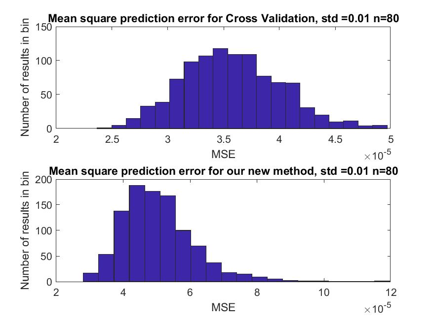
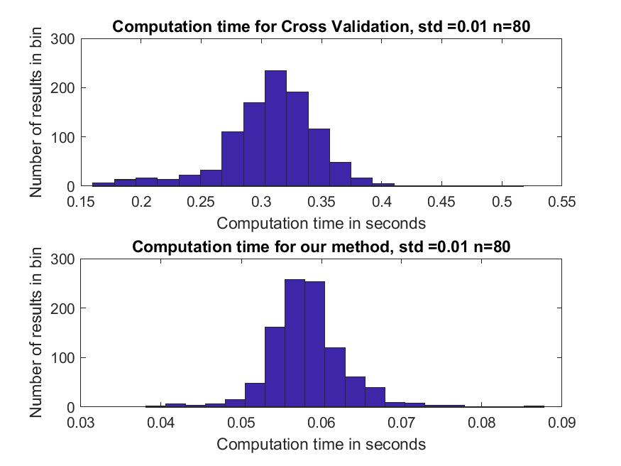
Figure 1. The top figure shows the $1/\sqrt{n}$ normalised least squares prediction error for the Cross Validation approach and the bottom figure shows the same prediction error for our method based on 1000 Monte Carlo experiments.

Figure 2. The top figure shows the computation time for the Cross Validation approach and the bottom figure shows the computation time for our method for the same experiments based on 1000 Monte Carlo trials.

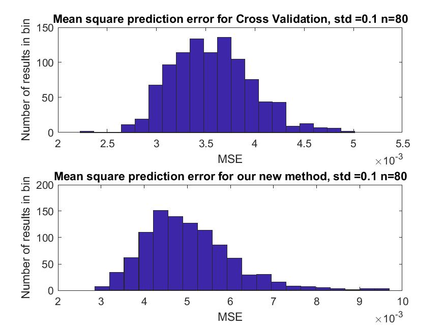
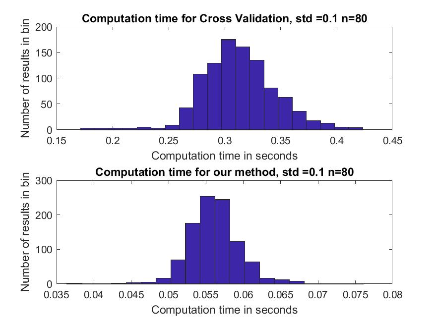
Figure 3. The top figure shows the $1/\sqrt{n}$ normalised least squares prediction error for the Cross Validation approach and the bottom figure shows the same prediction error for our method based on 1000 Monte Carlo experiments.

Figure 4. The top figure shows the computation time for the Cross Validation approach and the bottom figure shows the computation time for our method for the same experiments based on 1000 Monte Carlo trials.

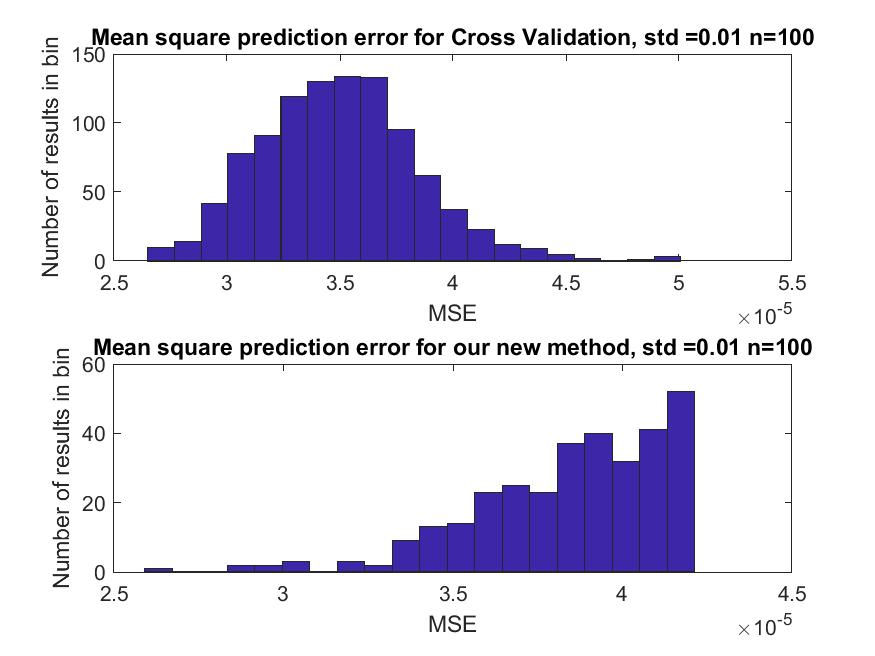
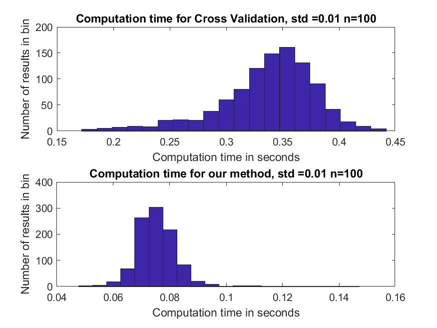
Figure 5. The top figure shows the $1/\sqrt{n}$ normalised least squares prediction error for the Cross Validation approach and the bottom figure shows the same prediction error for our method based on 1000 Monte Carlo experiments.

Figure 6. The top figure shows the computation time for the Cross Validation approach and the bottom figure shows the computation time for our method for the same experiments based on 1000 Monte Carlo trials.

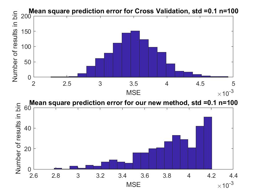
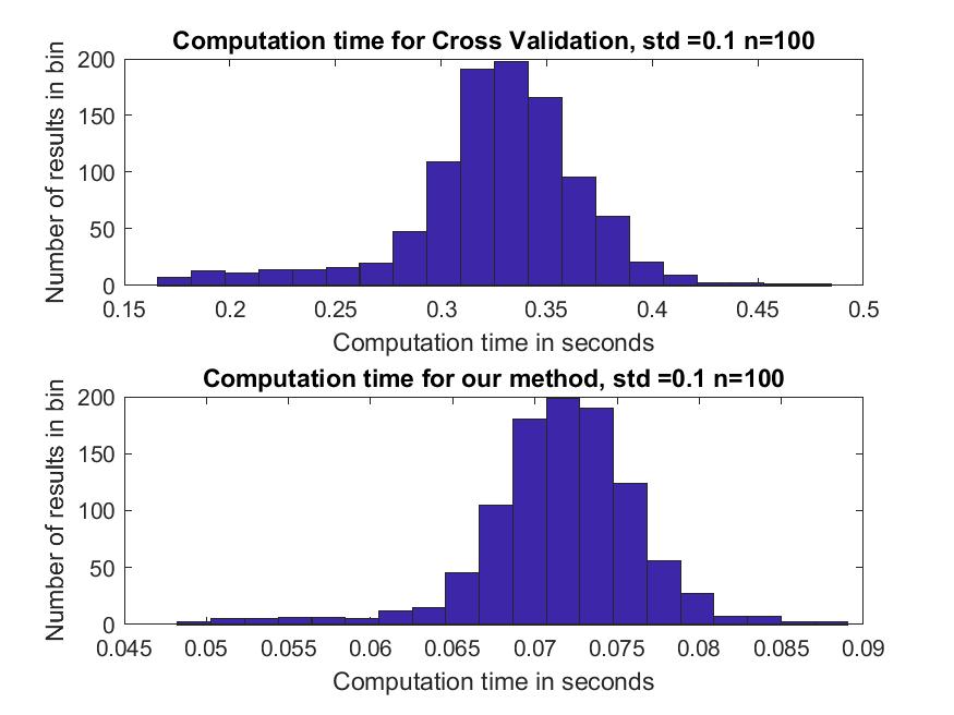
Figure 7. The top figure shows the $1/\sqrt{n}$ normalised least squares prediction error for the Cross Validation approach and the bottom figure shows the same prediction error for our method based on 1000 Monte Carlo experiments.

Figure 8. The top figure shows the computation time for the Cross Validation approach and the bottom figure shows the computation time for our method for the same experiments based on 1000 Monte Carlo trials.

3.2. Comparison with Cross Validation: A gene expression design

We also performed several experiments with the LASSO based on a highly correlated design previously studied in [13] and [14]. The columns of the design matrix are the expression of 34 genes for 100 patients.

Figure 10, 12 and 14 show the comparison results for the MSE and computational times for the Cross Validation procedure and our new method. Figure 10 (resp. Figure 12, Figure 14) presents the results for a noise level $\sigma$ equal to .1, (resp. .01, .001). As in the case of a random design, our approach is much faster than the optimised routine available in Matlab, despite the fact that our implementation uses quite basic Matlab coding.

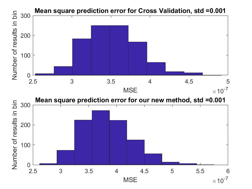
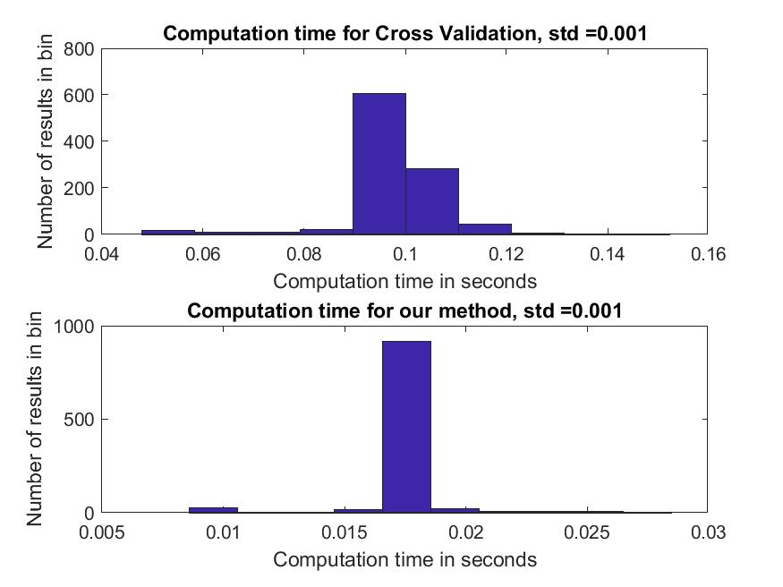
Figure 9. The top figure shows the $1/\sqrt{n}$ normalised least squares prediction error for the Cross Validation approach and the bottom figure shows the same prediction error for our method based on 1000 Monte Carlo experiments.

Figure 10. The top figure shows the computation time for the Cross Validation approach and the bottom figure shows the computation time for our method for the same experiments based on 1000 Monte Carlo trials.

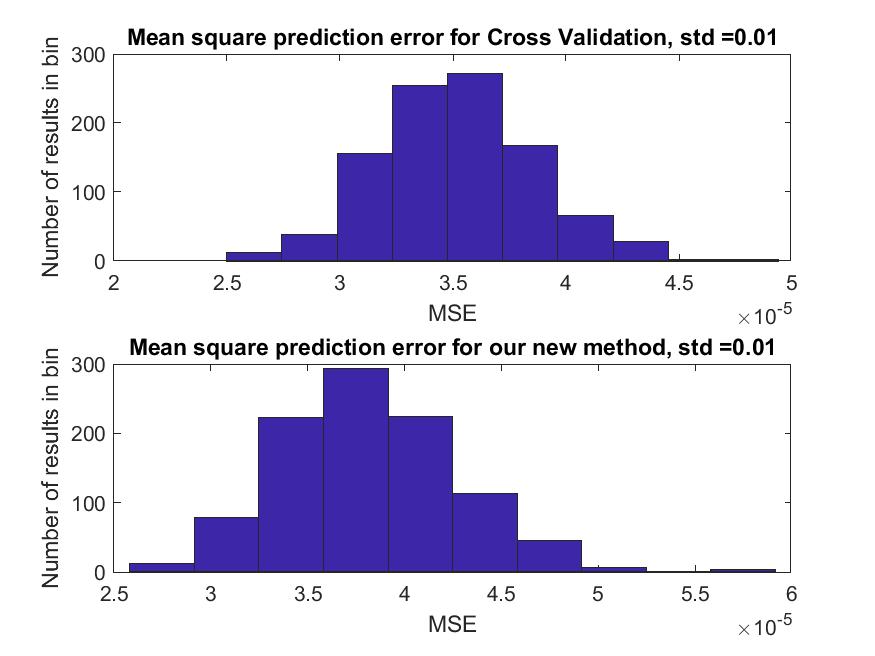
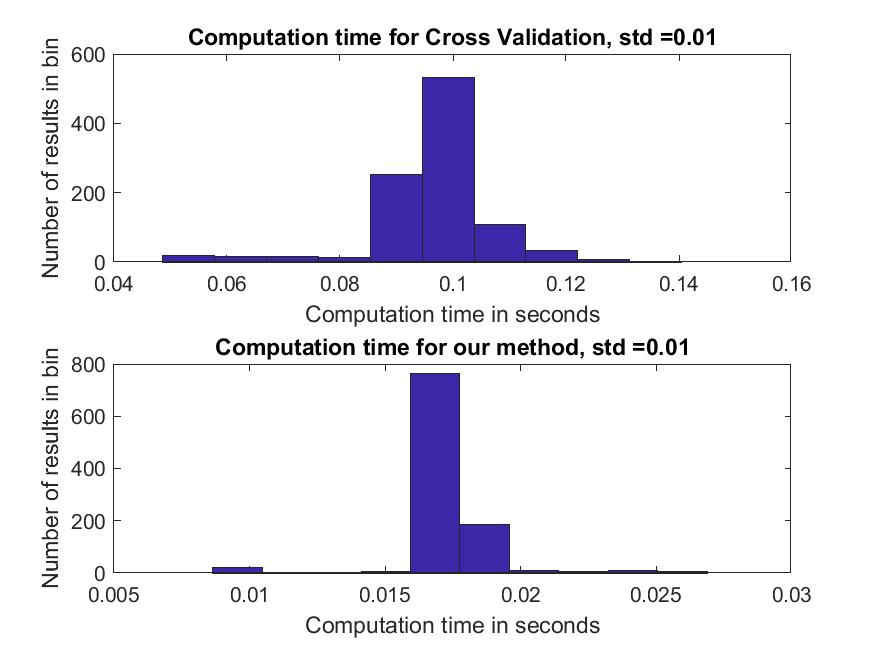
Figure 11. The top figure shows the $1/\sqrt{n}$ normalised least squares prediction error for the Cross Validation approach and the bottom figure shows the same prediction error for our method based on 1000 Monte Carlo experiments.

Figure 12. The top figure shows the computation time for the Cross Validation approach and the bottom figure shows the computation time for our method for the same experiments based on 1000 Monte Carlo trials.

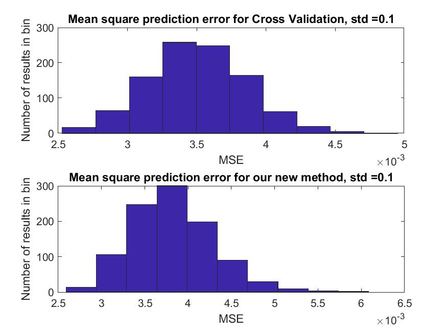
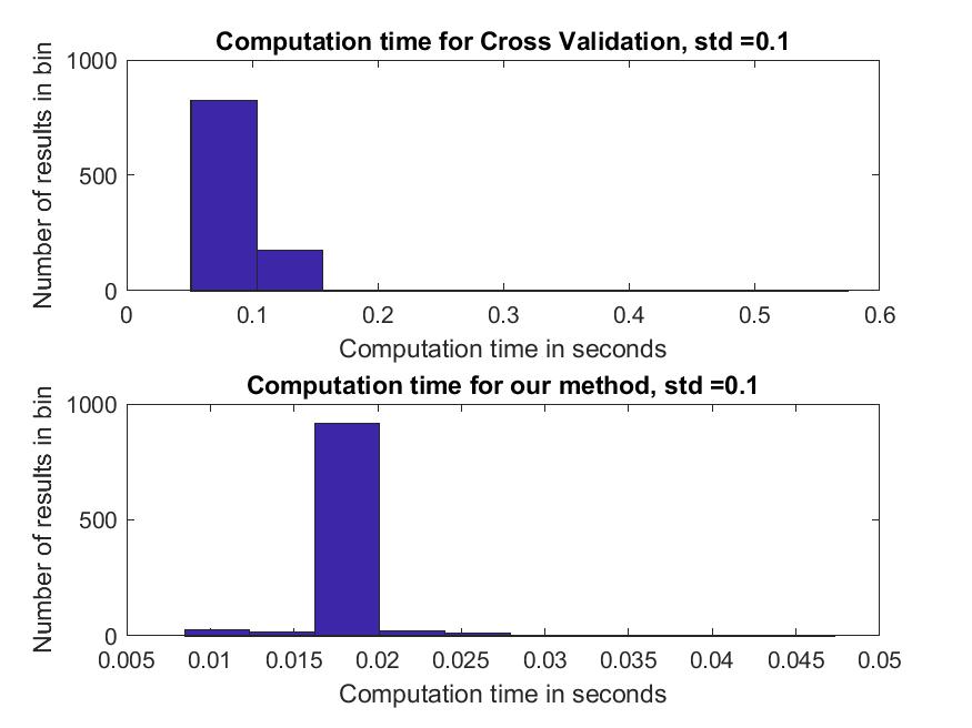
Figure 13. The top figure shows the $1/\sqrt{n}$ normalised least squares prediction error for the Cross Validation approach and the bottom figure shows the same prediction error for our method based on 1000 Monte Carlo experiments.

Figure 14. The top figure shows the computation time for the Cross Validation approach and the bottom figure shows the computation time for our method for the same experiments based on 1000 Monte Carlo trials.

4. Conclusion and future work

This short note presents a simple to implement method for choosing the hyper-parameter in the LASSO estimator. Application of this method can also easily be extended to various other models, such as two-stage estimation [10], [33], generalised linear models [30], graphical models [25], clustering [19], Robust PCA [6], etc.

One of the interesting features of the method is that it is potentially robust with respect to dependencies between the observations and event adversarial noise; see [9]. More results in this direction as well as a theoretical analysis the method will be included in future developments of this preliminary study.

References

- [1] Sylvain Arlot, Alain Celisse, et al., A survey of cross-validation procedures for model selection, Statistics surveys 4 (2010), 40–79.
- [2] Sanjeev Arora, Elad Hazan, and Satyen Kale, The multiplicative weights update method: a meta-algorithm and applications., Theory of Computing 8 (2012), no. 1, 121–164.
- [3] Stephen Becker, Jérôme Bobin, and Emmanuel J Candès, Nesta: a fast and accurate first-order method for sparse recovery, SIAM Journal on Imaging Sciences 4 (2011), no. 1, 1–39.
- [4] Peter Bühlmann and Sara Van De Geer, Statistics for high-dimensional data: methods, theory and applications, Springer Science & Business Media, 2011.
- [5] Emmanuel J Candes, Modern statistical estimation via oracle inequalities, Acta numerica 15 (2006), 257–325.
- [6] Emmanuel J Candès, Xiaodong Li, Yi Ma, and John Wright, Robust principal component analysis?, Journal of the ACM (JACM) 58 (2011), no. 3, 11.
- [7] Emmanuel J Candès, Yaniv Plan, et al., Near-ideal model selection by l1 minimization, The Annals of Statistics 37 (2009), no. 5A, 2145–2177.
- [8] Emmanuel J Candès, Justin Romberg, and Terence Tao, Robust uncertainty principles: Exact signal reconstruction from highly incomplete frequency information, IEEE Transactions on information theory 52 (2006), no. 2, 489–509.
- [9] Nicolo Cesa-Bianchi and Gábor Lugosi, Prediction, learning, and games, Cambridge university press, 2006.
- [10] StÉphane Chretien, An alternating approach to the compressed sensing problem, IEEE Signal Processing Letters 17 (2010), no. 2, 181–184.
- [11] Stéphane Chrétien and Sébastien Darses, Invertibility of random submatrices via tail-decoupling and a matrix chernoff inequality, Statistics & Probability Letters 82 (2012), no. 7, 1479–1487.
- [12] by same author, Sparse recovery with unknown variance: a lasso-type approach, IEEE Transactions on Information Theory 60 (2014), no. 7, 3970–3988.
- [13] Stephane Chretien, Christophe Guyeux, Michael Boyer-Guittaut, Regis Delage-Mouroux, and Francoise Descotes, Investigating gene expression array with outliers and missing data in bladder cancer, Bioinformatics and Biomedicine (BIBM), 2015 IEEE International Conference on, IEEE, 2015, pp. 994–998.
- [14] Stéphane Chrétien, Christophe Guyeux, Bastien Conesa, Régis Delage-Mouroux, Michèle Jouvenot, Philippe Huetz, and Françoise Descôtes, A bregman-proximal point algorithm for robust non-negative matrix factorization with possible missing values and outliers-application to gene expression analysis, BMC bioinformatics 17 (2016), no. 8, 284.
- [15] David L Donoho, Compressed sensing, IEEE Transactions on information theory 52 (2006), no. 4, 1289–1306.
- [16] Charles Dossal, Maher Kachour, MJ Fadili, Gabriel Peyré, and Christophe Chesneau, The degrees of freedom of the lasso for general design matrix, Statistica Sinica (2013), 809–828.
- [17] Yoav Freund and Robert E Schapire, A desicion-theoretic generalization of on-line learning and an application to boosting, Computational learning theory, Springer, 1995, pp. 23–37.
- [18] Caroline Giacobino, Sylvain Sardy, Jairo Diaz Rodriguez, and Nick Hengartner, Quantile universal threshold for model selection, arXiv preprint arXiv:1511.05433 (2015).
- [19] Toby Dylan Hocking, Armand Joulin, Francis Bach, and Jean-Philippe Vert, Clusterpath an algorithm for clustering using convex fusion penalties, 28th international conference on machine learning, 2011, p. 1.
- [20] Martin Jaggi, Revisiting frank-wolfe: Projection-free sparse convex optimization., ICML (1), 2013, pp. 427–435.
- [21] Seung-Jean Kim, Kwangmoo Koh, Stephen Boyd, and Dimitry Gorinevsky, ell_1 trend filtering, SIAM review 51 (2009), no. 2, 339–360.
- [22] Jean Lafond, Hoi-To Wai, and Eric Moulines, Convergence analysis of a stochastic projection-free algorithm, arXiv preprint arXiv:1510.01171 (2015).
- [23] Michael Lustig, David L Donoho, Juan M Santos, and John M Pauly, Compressed sensing mri, IEEE signal processing magazine 25 (2008), no. 2, 72–82.
- [24] Mathurin Massias, Alexandre Gramfort, and Joseph Salmon, Dual extrapolation for faster lasso solvers, arXiv preprint arXiv:1802.07481 (2018).
- [25] Nicolai Meinshausen and Peter Bühlmann, High-dimensional graphs and variable selection with the lasso, The annals of statistics (2006), 1436–1462.
- [26] Eugene Ndiaye, Olivier Fercoq, Alexandre Gramfort, Vincent Leclère, and Joseph Salmon, Efficient smoothed concomitant lasso estimation for high dimensional regression, Journal of Physics: Conference Series, vol. 904, IOP Publishing, 2017, p. 012006.
- [27] Neal Parikh, Stephen P Boyd, et al., Proximal algorithms., Foundations and Trends in optimization 1 (2014), no. 3, 127–239.
- [28] Robert Tibshirani, Regression shrinkage and selection via the lasso, Journal of the Royal Statistical Society. Series B (Methodological) (1996), 267–288.
- [29] Ryan J Tibshirani, Dykstra’s algorithm, admm, and coordinate descent: Connections, insights, and extensions, Advances in Neural Information Processing Systems, 2017, pp. 517–528.
- [30] Sara A Van de Geer et al., High-dimensional generalized linear models and the lasso, The Annals of Statistics 36 (2008), no. 2, 614–645.
- [31] Huahua Wang and Arindam Banerjee, Online alternating direction method (longer version), arXiv preprint arXiv:1306.3721 (2013).
- [32] Wotao Yin, Stanley Osher, Donald Goldfarb, and Jerome Darbon, Bregman iterative algorithms for -minimization with applications to compressed sensing, SIAM Journal on Imaging sciences 1 (2008), no. 1, 143–168.
- [33] Tong Zhang, Analysis of multi-stage convex relaxation for sparse regularization, Journal of Machine Learning Research 11 (2010), no. Mar, 1081–1107.
- [34] Hui Zou, Trevor Hastie, Robert Tibshirani, et al., On the "degrees of freedom" of the lasso, The Annals of Statistics 35 (2007), no. 5, 2173–2192.