Unsupervised learning for concept detection in medical images: a comparative analysis

Abstract

As digital medical imaging becomes more prevalent and archives increase in size, representation learning exposes an interesting opportunity for enhanced medical decision support systems. On the other hand, medical imaging data is often scarce and short on annotations. In this paper, we present an assessment of unsupervised feature learning approaches for images in the biomedical literature, which can be applied to automatic biomedical concept detection. Six unsupervised representation learning methods were built, including traditional bags of visual words, autoencoders, and generative adversarial networks. Each model was trained, and their respective feature space evaluated using images from the ImageCLEF 2017 concept detection task. We conclude that it is possible to obtain more powerful representations with modern deep learning approaches, in contrast with previously popular computer vision methods. Although generative adversarial networks can provide good results, they are harder to succeed in highly varied data sets. The possibility of semi-supervised learning, as well as their use in medical information retrieval problems, are the next steps to be strongly considered.

1 Introduction

In an era of a steadly increasing use of digital medical imaging, image recognition poses an interesting prospect for novel solutions supporting clinicians and researchers. In particular, the representation learning field is growing fast in recent years [1], and many of the breakthroughs in this field are occurring in deep learning methods, which have also been strongly considered in healthcare [2]. Leveraging representation learning tools to the medical imaging field is feasible and worthwhile, as they can provide additional levels of introspection of clinical cases through content-based image retrieval (CBIR).

Multiple initiatives for the provision of medical imaging data sets exist, the process of annotating the data with useful information is exhaustive and requires medical expertise, as it often nails down to a medical diagnosis. In the face of few to no annotations, unsupervised learning stands as a possible means of feature extraction for a measurement of relevance, leading to more powerful information retrieval and decision support solutions in digital medical imaging.

Although unsupervised representation is limited for specific classification tasks when compared to supervised learning approaches, the latter requires an exhaustive process from experts to obtain annotated content. Unsupervised learning, which avoids this issue, can also provide a few other benefits, including transferrability to other problems or domains, and can often be bridged to supervised and semi-supervised techniques. We have hypothesized that a sufficiently powerful representation of images would enable a medical imaging archive to automatically detect biomedical concepts with some level of certainty and efficiency, thus improving the system’s information retrieval capabilities over non-annotated data.

In this work, we present an assessment of unsupervised mid-level representation learning approaches for images in the biomedical literature. Representations are built using an ensemble of images from biomedical literature. The learned representations were validated with a brief qualitative feature analysis, and by training simple classifiers for the purpose of biomedical concept detection. We show that feature learning techniques based on deep neural networks can outperform techniques that were previously common-place in image recognition, and that models with adversarial networks, albeit harder to train, can improve the quality of feature learning.

2 Related Work

Representation learning, or feature learning, can be defined as the process of learning a transformation from a data domain into a representation that makes other machine learning tasks easier to approach [1]. The concept of feature extraction can be employed when this mapping is obtained with handcrafted algorithms rather than learned from the original data in the distribution. Representation learning can be achieved using a wide range of methods, such as k-means clustering, sparse coding [3] and Restricted Boltzmann Machines (RBMs) [4]. In image recognition, algorithms based on bags of visual words have been prevalent, as they have shown superior results over other low-level visual feature extraction techniques [5], [6]. More recently however, image recognition has had a strong focus on deep learning techniques, often with impressive results. Among these, approaches based on autoencoders [7], [8] have been considered and are still prevalent to this day.

Research on representation learning is even more intense on the ground-breaking concept of generative adversarial networks (GANs) [9]. GANs devise a min-max game where a generator of “fake” data samples attempts to fool a discriminator network, which in turn learns to discriminate fake samples from real ones. As the two components mutually improve, the generator will ultimately produce visually-appealing samples that are similar to the original data. The impressive quality of the samples generated by GANs have led the scientific community into devising new GAN variants and applications to this adversarial loss, including for feature learning [10].

Representation learning has been notably used in medical image retrieval, although even in this decade, handcrafted visual feature extraction algorithms are frequently considered in this context [11], [12]. Nonetheless, although the interest in deep learning is relatively recent, a wide variety of neural networks have been studied for medical image analysis [13], as they often exhibit greater potential for the task [14]. The use of unsupervised learning techniques is also well regarded as a means of exploiting as much of the available medical imaging data as possible [15]. On the other hand, the amount of medical imaging data may be scarse for many use cases, which makes training deep neural networks a difficult process.

3 Methods

We have considered a set of unsupervised representation learning techniques, both traditional (as in, employing classic computer vision algorithms) and based on deep learning, for the scope of images in the biomedical domain. These representations were subsequently used for the task of biomedical concept detection. Namely:

• We have experimented with creating image descriptors using bags of visual words (BoWs), for two different visual keypoint extraction algorithms.

• With the use of modern deep learning approaches, we have designed and trained various deep neural network architectures: a sparse denoising autoencoder, (SDAE), a variational autoencoder (VAE), a bidirectional generative adversarial network (BiGAN), and an adversarial autoencoder (AAE).

3.1 Bags of Visual Words

For each data set, images were converted to greyscale without resizing and visual keypoint descriptors were subsequently extracted. We employed two keypoint extraction algorithms separately: Scale Invariant Feature Transform (SIFT) [16], and Oriented FAST and Rotated BRIEF (ORB) [17]. While both algorithms obtain scale and rotation invariant descriptors, ORB is known to be faster and require less computational resources. The keypoints were extracted and their respective descriptors computed using OpenCV [18]. Each image would yield a variable number of descriptors of fixed size (128-dimensional for SIFT, 32-dimensional for ORB). In cases where the algorithm did not retrieve any keypoints, the algorithm’s parameters were adjusted to loosen edge detection criteria. All procedures described henceforth are the same for both ORB and SIFT keypoint descriptors.

From the training set, 3000 files were randomly chosen and their respective keypoint descriptors collected to serve as template keypoints. A visual vocabulary (codebook) of size $k=512$ was then obtained by performing k-means clustering on all template keypoint descriptors and retrieving the centroids of each cluster, yielding a list of 512 keypoint descriptors $\mathcal{V}=\{V_{i}\}$.

Once a visual vocabulary was available, we constructed an image’s BoW by determining the closest visual vocabulary point and incrementing the corresponding position in the BoW for each image keypoint descriptor. In other words, for an image’s BoW $B=\{o_{i}\}$, for each image keypoint descriptor $d_{j}$, $o_{i}$ is incremented when the smallest Euclidean distance from $d_{j}$ to all other visual vocabulary points in $V$ is the distance to $V_{i}$. Finally, each BoW was normalized so that all elements lie between 0 and 1. We can picture the bag of visual words as a histogram of visual descriptor occurrences, which can be used as a global image descriptor [19].

3.2 Deep Representation Learning

Modern representation techniques often rely on deep learning methods. We have considered a set of deep convolutional neural network architectures for inferring a late feature space over biomedical images. These models are composed of parts with very similar numbers of layers and parameters, in order to obtain a fairer comparison in the evaluation phase. This also means that the models will have very similar prediction times.

Training samples were obtained through the following process: images were resized so that its shorter dimension (width or height) was exactly $s_{g}$ pixels. Afterwards, the sample was augmented by feeding the networks random crops of size $s\times s$ (out of 9 possible kinds of crops: 4 corners, 4 edges and center). Validation images were resized to fit the $s\times s$ dimensions. For all cases, the images’ pixel RGB values were normalized to fit in the range [-1, 1]. Unless otherwise mentioned, the networks assumed a rescale size to $s_{g}=96$ and a crop size $s=64$.

Models with an enconding or discrimination process for visual data were based on the same convolutional neural network architecture, described in Table LABEL:tbl:enc and Table LABEL:tbl:dec. These models were influenced by the work in deep convolutional generative adversarial networks [20]. Each encoder layer is composed of a 2D convolution, followed by an optional (case-dependent) normalization algorithm and a model-dependent non-linearity. At the top of the network, global average pooling is performed, followed by a fully connected layer, yielding the code tensor $z$. The Details column in both tables may include the normalization and activation layers that follow a convolution layer.

Tbl. 1: A tabular representation of the SimpleNet layers’ specifications. The Details column may include the normalization and activation layers that follow a convolution layer (where LN stands for layer normalization and ReLU is the rectified linear unit $max(0,x)$).

Layer Kernels Size/Stride Details conv1 64 5x5 /2 Normalization + Non-Linearity conv2 128 5x5 /2 Normalization + Non-Linearity conv3 256 5x5 /2 Normalization + Non-Linearity conv4 512 5x5 /2 Normalization + Non-Linearity conv5 512 5x5 /2 Normalization + Non-Linearity avgpool N/A N/A fc $nb$ Linear activation

The decoding blocks replicate the encoding process in inverse order (Table LABEL:tbl:dec). It starts with a fully connected network from the latent (or prior) code vector into a series of convolutional layers. Convolutions in these blocks are transposed (also called fractionally-strided convolution in literature, and deconvolution in a few other papers). The weights of the network were randomly initialized with a Gaussian distribution.

Tbl. 2: A tabular representation of the decoder/generator layers’ specifications. The Details column may include the normalization and activation layers that follow a convolution layer.

Layer	Kernels	Size /stride	Details
fc	4096		Reshaped to 1024x2x2
dconv5	512	5x5 /2	Normalization + ReLU
dconv4	256	5x5 /2	Normalization + ReLU
dconv3	128	5x5 /2	Normalization + ReLU
dconv2	64	5x5 /2	Normalization + ReLU
dconv1	3	5x5 /2	Linear activation

3.2.1 Sparse Denoising Autoencoder

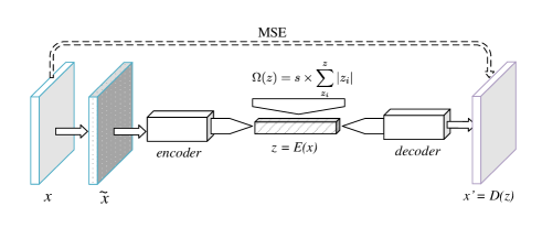
Fig. 1: Diagram of the sparse denoising autoencoder.

The first tested deep neural network model is a common autoencoder with denoising and sparsity constraints (Figure 1). In the training phase, a Gaussian noise of standard deviation 0.05 was applied over the input, yielding a noisy sample $\tilde{x}$. As a denoising autoencoder, its goal is to learn the pair of functions $(E,D)$ so that $x^{\prime}=D(E(\tilde{x}))$ is closest to the original input $x$. The aim of making $E$ a function of $\tilde{x}$ is to force the process to be more stable and robust, thus leading to higher quality representations [7].

Sparsity was achieved with two mechanisms. First, a rectified linear unit (ReLU) activation was used after the last fully connected layer of the encoder, turning negative outputs from the previous layer into zeros. Second, an absolute value penalization was applied to $z$, thus adding the extra minimization goal of keeping the code sum small in magnitude. The final decoder loss function was therefore:

$$\mathcal{L}(E,D)=\frac{1}{r}\sum^{\mathrm{r}}_{i=0}{\left(x_{i}-x_{i}^{\prime}\right)}^{2}+\Omega(z)$$

where

$$\Omega(z)=s\times\sum^{z}_{z_{i}}{z_{i}}$$

is the sparsity penalty function, $\mathrm{r}=64\times 64$ is the number of pixels in the input images, and $x$ represents the original input without synthesized noise. $s$ is the sparsity coefficient, which we left defined as $s=0.0001$. This network used batch normalization [21] and (non-leaking) ReLU activations.

3.2.2 Variational Autoencoder

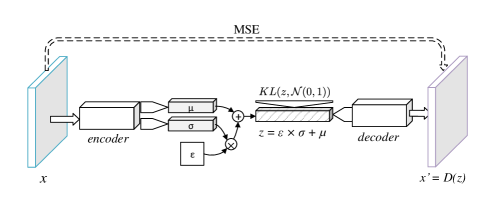
Fig. 2: Diagram of the variational autoencoder.

The encoder of the variational autoencoder (Figure 2) learns a stochastic distribution which can be sampled from, by minimizing the Kulback-Leibler divergence with a unitary normal distribution [8]. Like in the SDAE, convolutions were followed by batch normalization [21] and (non-leaking) ReLU activations.

3.2.3 Bidirectional GAN

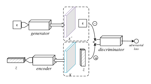
Fig. 3: Diagram of the bidirectional GAN.

While GANs are known to show great potential for representation purposes, the basic GAN archicture does not provide a means to encode samples to their respective prior. The bidirectional GAN, depicted in Figure 3, addresses this concern by including an encoder component, which learns the inverse process of the generator [10]. Rather than only observing data samples, the BiGAN discriminator’s loss function depends on the code-sample pair.

The Encoder component of the network used the same design as the discriminator, with the exception that the original data was fed with a size $s$ of 112, the outcome of cropping the data after the shortest dimension was resized to 128 pixels (as in, $s_{g}=128$ for the encoder). Images were still downsampled to 64x64 to be fed to the discriminator. Like in [10], all constituent parts of the GAN were optimized simultaneously in each iteration. The encoder and the discriminator of this model used layer normalization [22] and leaky ReLU with a leaking factor of 0.2 on all except the last respective convolutional layers.

3.2.4 Adversarial Autoencoder

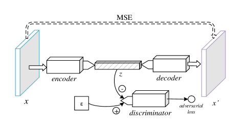
Fig. 4: Diagram of the adversarial autoencoder.

The adversarial autoencoder (AAE) is an autoencoder in which a discriminator is added to the bottleneck vector [23]. While reducing the $L_{2}$-norm distance between a sample and its decoded form, the full network includes an adversarial loss for distinguishing the encoder’s output from a stochastic prior code, thus serving as a regularizer to the encoding process.

Our AAE used a simple code discriminator composed of 2 fully connected layers of 128 units with a leaky ReLU activation for the first two layers, followed by a single neuron without a non-linearity. During training, the discriminator is fed a prior $z$ sampled from a random normal distribution $\mathcal{N}(0,1)$ as the real code, and the output of the encoder $E(x)$ as the fake code. The model uses layer normalization [22] on all except the last layers of each component, and leaky ReLU with a leaking factor of 0.2. Like in [10], all three components’ parameters were updated simultaneously in each iteration.

3.2.5 Network Training Details

The networks were trained through stochastic gradient descent, using the Adam optimizer [24]. The $\alpha_{1}$ hyperparameter was set to 0.5 for the BiGAN and the AAE, and 0.9 for the remaining networks.

Each neural network model was trained over 206000 steps, which is approximately 100 epochs, with a mini-batch size of 64. The base learning rate was 0.0005. The learning rate was multiplied by 0.2 halfway through the training process (50 epochs), to facilitate convergence.

All neural network training and latent code extraction was conducted using TensorFlow, and TensorBoard was used during the development for monitoring and visualization [25]. Depending on the particular model, training took on average 120 hours (a maximum of 215 hours, for the adversarial autoencoder) to complete on one of the GPUs of an NVIDIA Tesla K80 graphics card in an Ubuntu server machine.

3.3 Evaluation

The previously described methods for representation learning were aimed towards addressing the domain of biomedical images. A proper validation of these features was made with the use of the data sets from the ImageCLEF 2017 concept detection challenge [26]. As one of the sub-tasks of the caption prediction challenge, the goal of the challenge is to conceive a computer model for identifying the individual components from medical images, from which full captions could be composed. This task was accompanied with three data sets containing various images from biomedical journals: the training set (164614 images), the validation set (10000 images) and the testing set (10000 images). These sets were annotated with the lists of biomedical term identifiers from the UMLS (Unified Medical Language System) vocabulary for each image. The testing set’s annotations were hidden during the challenge, but were later on provided to participants.

Each of the set of features, learned from the approaches described in the previous section, were used to train simple classifiers for concept detection. In both cases, the same training and validation folds from the original data set were considered, after being mapped to their respective feature spaces. In addition, data points in the validation set with an empty list of concepts were discarded.

These simple models were used to predict the concept list of each image by sole observation of their respective feature set. Therefore, the assessment of our representation learning methods is made based on the effectiveness of capturing high-level features from latent codes alone.

3.3.1 Logistic Regression

Aiming for low complexity and classification speed, we performed logistic regression with stochastic gradient descent for concept detection, treating the UMLS terms as labels. More specifically, linear classifiers were trained over the features, one for each of the 750 (seven-hundred and fifty) most frequently occurring concepts in the training set. All models were trained using FTRL-Proximal optimization [27] with a base learning rate of $0.05$, an $L_{1}$-norm regularization factor of $0.001$, and a batch size of 128. Since the biomedical concepts are very sparse and imbalanced, the $F_{1}$ score was considered as the main evaluation metric, which was calculated with respect to multiple fixed operating point thresholds (namely, $0.025$, $0.05$, $0.075$, $0.1$, $0.125$, $0.15$, $0.175$, and $0.2$) for each sample and averaged across the 750 labels. The threshold which resulted in the highest mean $F_{1}$ score on the validation set is recorded, and the respective precision, recall, and area under the ROC curve were also included. Subsequently, the same model and threshold were used for predicting the concepts in the testing set, the $F_{1}$ score of which was retrieved with the official evaluation tool from the ImageCLEF challenge.

Since it is also possible to combine multiple representations with simple vector concatenation, we have experimented training these classifiers using a mixture of features from the SDAE and AAE latent codes. This process is often called early fusion, and is contrasted with late fusion, which involves merging the results of separate models. Each model undertook a few dozens of training epochs until the best $F_{1}$ score among the thresholds would no longer improve. In practice, training and evaluation of the linear classifiers was done with TensorFlow.

3.3.2 $k$-nearest neighbors

A relevant focus of interest in representation learning is its potential in information retrieval. While concept detection is not a retrieval problem, and the use of retrieval techniques is a naive approach to classification, it is fast and scales better in the face of multiple classes. Furthermore, it enables a rough assessment of whether the representation would fare well in retrieval tasks where similarity metric were not previously learned, which is the case for the Euclidean distance between features.

A modified form of the k-nearest neighbors algorithm was used as a second means of evaluation. Each data point in the validation set had its concepts predicted by retrieving the $n$ closest points from the training feature set (henceforth called neighbors) in Euclidean space and accumulating all concepts of those neighbors into a boolean sum of labels. This tweak makes the algorithm more sensitive to very sparse classification labels, such as those found in the biomedical concept detection task. All natural numbers from 1 to 5 were tested for the possible $k$ number of neighbors to consider. Analogous to the logistic regression above, the $k$ which resulted in the highest $F_{1}$ score on the validation set was regarded as the optimal parameter, and predictions over the testing set were evaluated using the optimal $k$.
The actual search for the nearest neighbors was performed using the Faiss library, which contributed to a rapid retrieval [28]. Feature fusion was not considered in the results, as they did not seem to bring any improvement over singular representations.

4 Results

4.1 Qualitative results

Each representation learning approach described in this work resulted in a 512-dimensional feature space. Figure 5 shows the result of mapping the validation feature set of each representation learned into a two-dimensional space, using principal component analysis (PCA). The three primary colors were used (red, green, and blue) to label the points with the three most commonly occurring UMLS terms in the training set, namely C1696103 (Image-dosage form), C0040405 (X-Ray Computed Tomography), and C0221198 (Lesion), each painted in an additive fashion.

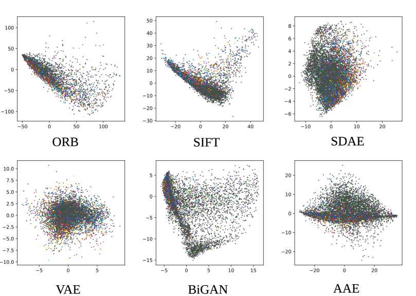
Fig. 5: The 2D projections of the latent codes in the validation set, for each learned feature space. Best seen in color.

While extreme outliers were removed from the figures, it can be noted that the ORB, SIFT and BiGAN representations had more outliers than the other three representations. A good representation would enable samples to be linearly separable based on their list of concepts. Even though the concept detection task is too hard for a clear cut separation, one can still identify regions in the manifold in which points of one of the frequent labels are mostly gathered. The existence of concentrations of random points in certain parts of the manifold, as further observed from the classification results, is noticeable mostly in poorer quality representations.

The latent space regularization in representations based on deep learning is also apparent in these plots: both the AAE (with the approximate Jason-Shennen divergence from the adversarial loss) and the VAE (with the Kulback-Leibler divergence) manifest a distribution that is close to a normal distribution.

4.2 Linear Classifiers

Table LABEL:tbl:logreg shows the best resulting metrics obtained with logistic regression on the validation set, followed by the final score on the testing set. Mix is the identifier given for the feature combination of SDAE and AAE. We observed that, for all classifiers, the threshold of 0.075 would yield the best $F_{1}$ score. This metric, when obtained with the validation set, assumes the existence of only the 750 most frequent concepts in the training set. Nonetheless, these metrics are deemed acceptable for a quantitative comparison among the trained representations, and have indeed established the same score ordering as the metrics in the testing set. The adversarial autoencoder obtained the best mean $F_{1}$ score in concept detection, only superseded with a combination of the same features with those from the sparse denoising autoencoder.

These metrics, although seemingly low, are within the expected range of scores in the domain of concept detection in biomedical images, since the classified labels are very scarce. As an example, only 10.9% of the training set is positive for the most frequent term. For the second and third most frequent terms, the numbers are 9.8% and 8.6% respectively. The mean number of positive labels of each of the 750 most frequent concepts is 876.7, with a minimum of 203 positive labels for the 750th most frequent concept in the training set. We find that most concepts in the set do not have enough images with a positive label for a valuable classifier.

The scores obtained here are on par with some of the results from the ImageCLEF 2017 challenge. The best $F_{1}$ scores on the testing set, without the use of external resources that could severely bias the results, were 0.1583 (with a pre-trained neural network model [29]) and 0.1436 (with no external resources [30]) [26]. The use of additional information outside of the given data sets is known to significantly improve the results. In the list of submissions where no external resources were used, these techniques were only outperformed by the submissions from the IPL team [26], [30]. While the work has also relied on building global unsupervised representations, our representations are significantly more compact in size, and thus more computationally efficient in practice.

Tbl. 3: The best metrics obtained from logistic regression for each representation learned, where Mix is the feature combination of SDAE and AAE.

Type	$F_{1}$ score	precision	recall	AUC	$F_{1}$ score (test)
ORB	0.13837	0.13438	0.14260	0.69922	0.09667
SIFT	0.13303	0.11877	0.15118	0.75285	0.09518
SDAE	0.15108	0.14142	0.16215	0.78065	0.10288
VAE	0.13970	0.13729	0.14220	0.75978	0.09236
BiGAN	0.14055	0.14244	0.13871	0.78067	0.09888
AAE	0.15891	0.14619	0.17406	0.78721	0.10797
Mix	0.16131	0.14704	0.17865	0.78865	0.11050

The combined representation of concatenating the feature spaces of the SDAE and AAE have resulted in even better classifiers. Although the results of the combined representation are shown here, this improvement is not to be overstated, given that it relies on a wider feature vector and on training two representations that were meant to perform individually. Another relevant observation is that the representations based on BoWs were generally less effective for the task than deep representation learning methods. Although SIFT BoWs have resulted in a slightly better area under the ROC curve, the chosen operating points led to ORB slighly outperforming SIFT.

It is understood that the thresholds can be better fine-tuned to further increase these numbers [31]. Rather than performing a methodic determination of the optimal threshold, we chose to avoid overfitting the validation set by selecting a few thresholds within the interval known to contain the optimal threshold.

4.3 $k$-Nearest Neighbors

The results of classifying the validation set with similarity search are presented in Table LABEL:tbl:knn. The presence of lower $F_{1}$ scores than those with linear classifiers is to be expected: the linear classifier can be interpreted as a model which learns a custom distance metric for each label, whereas $k$-NN relies on a fixed Euclidean distance metric. With $k$-nearest neighbors, the best mean $F_{1}$ score of 0.07505 was obtained with the SDAE. The AAE follows with a mean $F_{1}$ score of 0.06910. The form of passive fitting over the validation set, from the choice of $k$, is much less greedy than the training process of the logistic regression, which included a choice of operating threshold and halting condition based on the outcome from the validation set. Therefore, it is expected that the final $F_{1}$ score on the testing set heavily resembles the values obtained on the validation set.

Tbl. 4: The best $F_{1}$ scores obtained from vector similarity search for each representation learned.

Type	$F_{1}$ score	precision	recall	AUC	k	$F_{1}$ score (test)
ORB	0.04279	0.02990	0.10575	0.55240	4	0.04177
SIFT	0.05980	0.04341	0.13402	0.56660	3	0.05665
SDAE	0.07995	0.06954	0.12041	0.55998	2	0.07505
VAE	0.03569	0.02490	0.08703	0.54307	4	0.03450
BiGAN	0.04700	0.03496	0.09928	0.54926	3	0.04733
AAE	0.07212	0.06263	0.10898	0.55427	2	0.06910

5 Conclusion

This paper takes unsupervised representation learning techniques from state-of-the-art, facing them against a more traditional bags of visual words approach. The methods were evaluated with the biomedical concept detection sub-task of the ImageCLEF 2017 caption prediction task. We have tested the hypothesis that a powerful image descriptor can contribute to efficient concept detection with some level of certainty, without observing the original image. Results are presented for six different approaches, where two of them rely on visual keypoint extraction and description algorithms, and other two of them are based on generative adversarial networks. Overall, these methods have significantly outperformed our previous participation and are on par with other techniques in the challenge.

As identified in [32] and proved in this work, it is possible to obtain more powerful representations with modern deep learning approaches, in contrast with previously popular computer vision methods such as the SIFT bags of visual words. Deep learning techniques based on GANs can provide good results, but the additional complexity, the difficulty of convergence, and the possibility of mode collapse can significantly cripple their performance in representation learning. Nonetheless, these issues are already a high focus of attentions at this time, and will likely lead to substantial improvements in GAN design and training.

It is also important that these approaches are augmented with non-visual information. In particular, a medical imaging archive should take the most advantage of the available data beyond pixel data. Future work will consider semi-supervised learning as a means of building more descriptive representations from known categories and other annotations. Subsequently, these representations are to be evaluated in a medical information retrieval scenario, as well as with other data sets in the medical imaging domain.

6 Acknowledgements

This work is financed by the ERDF - European Regional Development Fund through the Operational Programme for Competitiveness and Internationalisation - COMPETE 2020 Programme, and by National Funds through the FCT – Fundação para a Ciência e a Tecnologia, within project PTDC/EEI-ESS/6815/2014. Eduardo Pinho is funded by the FCT under the grant PD/BD/105806/2014.

References

[1] Y. Bengio, A. Courville, and P. Vincent, “Representation learning: A review and new perspectives,” Pattern Analysis and Machine Intelligence, IEEE Transactions on, vol. 35, no. 8, pp. 1798–1828, 2013.

[2] D. Ravi et al., “Deep Learning for Health Informatics,” Biomedical and Health Informatics, IEEE Journal of, vol. 21, no. 1, pp. 4–21, Jan. 2017.

[3] H. Lee, A. Battle, R. Raina, and A. Y. Ng, “Efficient sparse coding algorithms,” Advances in Neural Information Processing Systems, vol. 19, no. 2, pp. 801–808, 2006.

[4] G. E. Hinton, S. Osindero, and Y.-W. Teh, “A fast learning algorithm for deep belief nets,” Neural computation, vol. 18, no. 7, pp. 1527–1554, 2006.

[5] X. Wangming, W. Jin, L. Xinhai, Z. Lei, and S. Gang, “Application of Image SIFT Features to the Context of CBIR,” in International conference on computer science and software engineering, 2008, pp. 552–555.

[6] I. Dimitrovski, D. Kocev, I. Kitanovski, S. Loskovska, and S. Džeroski, “Improved medical image modality classification using a combination of visual and textual features,” Computerized Medical Imaging and Graphics, vol. 39, pp. 14–26, 2015.

[7] P. Vincent, H. Larochelle, I. Lajoie, Y. Bengio, and P.-a. Manzagol, “Stacked Denoising Autoencoders: Learning Useful Representations in a Deep Network with a Local Denoising Criterion,” Journal of Machine Learning Research, vol. 11, pp. 3371–3408, 2010.

[8] D. P. Kingma and M. Welling, “Auto-Encoding Variational Bayes,” pp. 1–14, 2014.

[9] I. J. Goodfellow et al., “Generative Adversarial Nets,” pp. 1–9, 2014.

[10] J. Donahue, P. Krähenbühl, and T. Darrell, “Adversarial feature learning,” arXiv preprint arXiv:1605.09782, May 2016.

[11] Z. Li, X. Zhang, H. Müller, and S. Zhang, “Large-scale Retrieval for Medical Image Analytics: A Comprehensive Review,” Medical Image Analysis, 2017.

[12] J. Kalpathy-Cramer, A. G. S. de Herrera, D. Demner-Fushman, S. Antani, S. Bedrick, and H. Müller, “Evaluating performance of biomedical image retrieval systems—an overview of the medical image retrieval task at ImageCLEF 2004–2013,” Computerized Medical Imaging and Graphics, vol. 39, pp. 55–61, 2015.

[13] G. Litjens et al., “A survey on deep learning in medical image analysis,” Medical Image Analysis, vol. 42, pp. 60–88, 2017.

[14] W. Sun, B. Zheng, and W. Qian, “Automatic feature learning using multichannel ROI based on deep structured algorithms for computerized lung cancer diagnosis,” Computers in biology and medicine, vol. 89, pp. 530–539, 2017.

[15] G. Wu, M. Kim, Q. Wang, B. C. Munsell, and D. Shen, “Scalable high-performance image registration framework by unsupervised deep feature representations learning,” IEEE Transactions on Biomedical Engineering, vol. 63, no. 7, pp. 1505–1516, 2016.

[16] D. G. Lowe, “Distinctive Image Features from Scale-Invariant Keypoints,” International Journal of Computer Vision, vol. 60, no. 2, pp. 91–110, 2004.

[17] E. Rublee, V. Rabaud, K. Konolige, and G. Bradski, “ORB: An efficient alternative to SIFT or SURF,” in Computer vision (ICCV), 2011 IEEE international conference on, 2011, pp. 2564–2571.

[18] G. Bradski and Others, “The OpenCV library,” Doctor Dobbs Journal, vol. 25, no. 11, pp. 120–126, 2000.

[19] J. Sivic and A. Zisserman, “Video google: A text retrieval approach to object matching in videos,” in Computer vision, 2003. Proceedings. Ninth IEEE international conference on, 2003, pp. 1470–1477.

[20] A. Radford, L. Metz, and S. Chintala, “Unsupervised Representation Learning with Deep Convolutional Generative Adversarial Networks,” arXiv preprint arXiv:1511.06434, pp. 1–16, 2016.

[21] S. Ioffe and C. Szegedy, “Batch Normalization: Accelerating Deep Network Training by Reducing Internal Covariate Shift,” arXiv preprint arXiv:1502.03167, pp. 1–11, 2015.

[22] J. L. Ba, J. R. Kiros, and G. E. Hinton, “Layer normalization,” Jul. 2016.

[23] A. Makhzani, J. Shlens, N. Jaitly, I. Goodfellow, and B. Frey, “Adversarial Autoencoders,” Nov. 2015.

[24] D. P. Kingma and J. L. Ba, “Adam: A Method for Stochastic Optimization,” in International conference on learning representations, 2015.

[25] M. Abadi et al., “TensorFlow: Large-Scale Machine Learning on Heterogeneous Distributed Systems,” Mar. 2016.

[26] C. Eickhoff, I. Schwall, A. de Herrera, and H. Müller, “Overview of ImageCLEFcaption 2017 - the image caption prediction and concept extraction tasks to understand biomedical images,” CLEF working notes, CEUR, 2017.

[27] H. B. McMahan et al., “Ad click prediction: a view from the trenches,” in Proceedings of the 19th acm sigkdd international conference on knowledge discovery and data mining, 2013, pp. 1222–1230.

[28] J. Johnson, M. Douze, and H. Jégou, “Billion-scale similarity search with GPUs,” arXiv preprint arXiv:1702.08734, 2017.

[29] K. Dimitris and K. Ergina, “Concept detection on medical images using Deep Residual Learning Network,” in Working notes of conference and labs of the evaluation forum, 2017.

[30] L. Valavanis and S. Stathopoulos, “IPL at ImageCLEF 2017 Concept Detection Task,” in Working notes of conference and labs of the evaluation forum, 2017.

[31] Z. C. Lipton, C. Elkan, and B. Narayanaswamy, “Thresholding Classifiers to Maximize F1 Score,” Machine Learning and Knowledge Discovery in Databases, vol. 8725, pp. 225—–239, Feb. 2014.

[32] E. Pinho, J. F. Silva, J. M. Silva, and C. Costa, “Towards Representation Learning for Biomedical Concept Detection in Medical Images: UA. PT Bioinformatics in ImageCLEF 2017,” in Working notes of conference and labs of the evaluation forum, 2017.