Quantum Spin probabilities at positive temperature are Hölder Gibbs probabilities

Abstract

We consider the KMS state associated to the Hamiltonian $H=\sigma^{x}\otimes\sigma^{x}$ over the quantum spin lattice $\mathbb{C}^{2}\otimes\mathbb{C}^{2}\otimes\mathbb{C}^{2}\otimes...$. For a fixed observable of the form $L\otimes L\otimes L\otimes...$, where $L:\mathbb{C}^{2}\to\mathbb{C}^{2}$ is self adjoint, and for positive temperature $T$ one can get a naturally defined stationary probability $\mu_{T}$ on the Bernoulli space $\{1,2\}^{\mathbb{N}}$. The Jacobian of $\mu_{T}$ can be expressed via a certain continued fraction expansion. We will show that this probability is a Gibbs probability for a Hölder potential. Therefore, this probability is mixing for the shift map. For such probability $\mu_{T}$ we will show the explicit deviation function for a certain class of functions. When decreasing temperature we will be able to exhibit the explicit transition value $T_{c}$ where the set of values of the Jacobian of the Gibbs probability $\mu_{T}$ changes from being a Cantor set to being an interval.

We also present some properties for quantum spin probabilities at zero temperature (for instance, the explicit value of the entropy).

1 Introduction

In [19] the case of zero temperature for the quantum spin probability and the Hamiltonian $H=\sigma^{x}\otimes\sigma^{x}$, where $\sigma_{x}$ is the $x$-Pauli matrix, was analyzed. Here we will analyze the analogous problem in the case of positive temperature.

Given a selfadjoint operator $H$ acting on a finite dimensional complex Hilbert space $\mathcal{H}$ and a temperature $T>0$, the density operator

$$\rho_{H,T}=\frac{e^{-\frac{1}{T}\,H}}{Z(T)},$$

where $Z(T)=$ Trace $e^{-\frac{1}{T}\,H}$, is called the KMS operator associated to the Hamiltonian $H$. It is usual to denote $\beta=1/T$. A general reference on KMS operators and KMS states is [5].

The set of linear operators acting on $\mathbb{C}^{2}$ will be denoted by $\mathcal{M}_{2}.$ We will call $\omega=\omega_{n}:\underbrace{\mathcal{M}_{2}\otimes\mathcal{M}_{2}\otimes...\otimes\mathcal{M}_{2}}_{n}\to\mathbb{C}$ a $C^{*}$-dynamical state if $\omega_{n}(I^{\otimes\,n})=1$ and $\omega_{n}(a)\geq 0$, if $a$ is a non-negative element in the tensor product. General references on tensor products and spin lattices are [11], [1] and [20].

Here we will consider the Hamiltonian $H=\sigma^{x}\otimes\sigma^{x}:\mathbb{C}^{2}\otimes\mathbb{C}^{2}\,\to\mathbb{C}^{2}\otimes\mathbb{C}^{2}$ acting on the spin lattice $\mathbb{C}^{2}\otimes\mathbb{C}^{2}\otimes\mathbb{C}^{2}\otimes...$, where

$$\sigma_{x}=\left(\begin{array}[]{cc}0&1\\ 1&0\end{array}\right)$$

is the $x$-Pauli matrix. More precisely we will consider for each $n\geq 2$ the state $\omega=\omega_{n}$, which is defined in the following way: consider a fixed value $\beta>0$, and $H_{n}=(\mathbb{C}^{2})^{\otimes n}\to(\mathbb{C}^{2})^{\otimes n}$ given by

$$H_{n}=\sum_{j=0}^{n-2}I^{\otimes\,j}\otimes H\otimes I^{\otimes\,(n-j-2)}.$$

Denote $\rho_{\omega}$ the operator

$$\rho_{\omega}=\rho_{\omega_{H,\beta,n}}=\frac{1}{Tr\,(e^{-\,\beta H_{n}})}e^{-\,\beta H_{n}}$$

and define the $C^{*}$-dynamical state $\omega_{n}=\omega_{H,\beta,n}$ by

$$\omega_{n}\,(A)\,=\text{ trace }\,\,(\rho_{\omega}\,A),\,\,\,\,A\in\underbrace{\mathcal{M}_{2}\otimes\mathcal{M}_{2}\otimes...\otimes\mathcal{M}_{2}}_{n}.$$

The family $w_{n}$, $n\in\mathbb{N}$, defines a $C^{*}$-dynamical state over $\mathcal{M}_{2}^{\otimes\,\infty}$ in the following sense: $w_{n}$ is a $C^{*}$-dynamical state over $\underbrace{\mathcal{M}_{2}\otimes\mathcal{M}_{2}\otimes...\otimes\mathcal{M}_{2}}_{n}$ for each $n$. The $C^{*}$-dynamical states play an important role in Quantum Statistical Mechanics (see [5] and [12])

Assumption A: We fix a value $\theta\in(0,\pi/2),\,\theta\neq\pi/4,$ and we consider the self-adjoint operator $L$ on the form

$$L=\,\left(\begin{array}[]{cc}\cos^{2}(\theta)-\sin^{2}(\theta)&2\cos(\theta)\sin(\theta)\\ 2\cos(\theta)\sin(\theta)&\sin^{2}(\theta)-\cos^{2}(\theta)\end{array}\right).$$

The case $\theta=0$ corresponds to $L=\sigma^{z}$ and the case $\theta=\pi/2$ corresponds to $L=-\sigma^{z}$. We will not consider these cases.

What is important in the above choice of $L$ is the corresponding subspaces of eigenvectors. The eigenvalues of $L$ are $\lambda_{1}=1$ and $\lambda_{2}=-1$ which are associated, respectively, to the unitary eigenvectors $\psi_{1}=(\cos(\theta),\sin(\theta))\in\mathbb{C}^{2}$ and $\psi_{2}=(-\sin(\theta),\cos(\theta))\in\mathbb{C}^{2}$, which are orthogonal. Furthermore, for any $n\in\mathbb{N}$, the observable

$$L^{\otimes\,n}:=(L\otimes L\otimes\,....\otimes L):(\mathbb{C}^{d}\otimes\mathbb{C}^{d}\otimes\,....\otimes\mathbb{C}^{d})\to(\mathbb{C}^{d}\otimes\mathbb{C}^{d}\otimes\,....\otimes\mathbb{C}^{d})$$

has the eigenvector $(\,\psi_{j_{1}}\otimes\psi_{j_{2}}\otimes....\otimes\psi_{j_{n}}\,)$ associated to the eigenvalue $\lambda_{j_{1}}\cdot\lambda_{j_{2}}\cdots\lambda_{j_{n}}.$ Any eigenvalue of $L^{\otimes\,n}$ is of this form.

We denote by $P_{j}=P_{\psi_{j}}:\mathbb{C}^{2}\to\mathbb{C}^{2}$ the orthogonal projection on the subspace generated by $\psi_{j}$,  $j\in\{1,2\}$. In this way

$$P_{1}=\,\left(\begin{array}[]{cc}\cos(\theta)^{2}&\cos(\theta)\,\sin(\theta)\\ \cos(\theta)\,\sin(\theta)&\sin(\theta)^{2}\end{array}\right)$$

and

$$P_{2}=\left(\begin{array}[]{cc}\sin(\theta)^{2}&-\cos(\theta)\,\sin(\theta)\\ -\cos(\theta)\,\sin(\theta)&\cos(\theta)^{2}\end{array}\right).$$

Note that Tr $P_{1}=$ Tr $P_{2}=1$. Moreover,

$$\sigma^{x}(P_{1})=\left(\begin{array}[]{cc}\cos(\theta)\sin(\theta)&\sin^{2}(\theta)\\ \cos^{2}(\theta)&\cos(\theta)\sin(\theta)\end{array}\right),$$

which has trace equal to $\beta_{1}:=\sin(2\,\theta)\in\mathbb{R}$, and

$$\sigma^{x}(P_{2})=\,\left(\begin{array}[]{cc}-\cos(\theta)\sin(\theta)&\cos^{2}(\theta)\\ \sin^{2}(\theta)&-\cos(\theta)\sin(\theta)\end{array}\right)$$

has trace $\beta_{2}:=-\sin(2\,\theta)\in\mathbb{R}$. Therefore, $\text{{Tr}}\,(\sigma^{x}(P_{2}))=\beta_{2}=-\beta_{1}$.

We want to define a probability $\mu_{\beta}$ on the Bernoulli space $\{1,2\}^{\mathbb{N}}.$ First, for each $n$ we introduce the probability $\mu_{\beta,n}$, in such way that, for an element $(j_{1},...,j_{n})\in\{1,2\}^{n}$ it is given by

$$\mu_{\beta,n}(j_{1},,...,j_{n})=\frac{1}{Tr\,(e^{-\,\beta H_{n}})}\text{{Tr}}\,\left[\,e^{-\,\beta H_{n}}(P_{{j_{1}}}\otimes P_{{j_{2}}}\otimes...\otimes P_{{j_{n}}})\right]=$$

$$\frac{1}{\cos^{n-1}(i\beta)2^{n}}\text{{Tr}}\,\left[\prod_{i=1}^{n-1}[\cos(i\beta)I^{\otimes n}+i\sin(i\beta)(\sigma^{x}_{i}\otimes\sigma^{x}_{i+1})_{n}](P_{j_{1}}\otimes...\otimes P_{j_{n}})\right],$$

where the above product represents composition of operators.

Finally we observe that there exists a unique probability $\mu_{\beta}$ over $\Omega=\{1,2\}^{\mathbb{N}}$ satisfying $\mu_{\beta}([j_{1},...,j_{n}])=\mu_{\beta,n}(j_{1},...,j_{n})$ for any $n\in\{2,3,...\}$ and any cylinder set $[j_{1},...,j_{n}]\subset\Omega$. It is also invariant for the shift map $\sigma$ (see Theorem 9 below).

Definition 1.

We call the above probability $\mu_{\beta}$ the quantum spin probability for inverse temperature $\beta$.

The above definition is consistent with the one usually considered on the literature (see [13], [14] and [15]).

Suppose $J:\{1,2\}^{\mathbb{N}}\to\mathbb{R}$ is a Hölder positive function such that for any $y\in\{1,2\}^{\mathbb{N}}$ we have that $\sum_{\{x\,|\,\sigma(x)=y\}}J(x)=1$. The associated Ruelle operator $\mathcal{L}_{\log J}$ is the one such that $\mathcal{L}_{\log J}(f)=g$, when for any $y$ we have

$$g(y)=\sum_{\{x\,|\,\sigma(x)=y\}}J(x)\,f(x).$$

$\mathcal{L}_{\log J}^{*}$ denotes the dual of the Ruelle operator which acts on probabilities over $\{1,2\}^{\mathbb{N}}$ (via the Riesz Theorem) as described in [22].

Definition 2.

The unique probability $m$ such that $\mathcal{L}_{\log J}^{*}(m)=m$ is called the Hölder Gibbs probability associated to $\log J$. We say that $J$ is the Jacobian of $m$.

One can show that the Kolomogorov entropy satisfies $h(m)=-\int\log Jdm.$ The function $J$ can also be seen as the Radon-Nykodim derivative on the inverse branches of $\sigma$ (see section 9.7 of [26] or [23]). Hölder Gibbs probabilities are equilibrium states for Hölder potentials (see [22]). The relation of Gibbs probabilities with DLR probabilities is explained in [7] and [6].

Our main result is the following (see section 4):

Theorem 3.

For any $\beta>0$ there exist a Holder function $J_{\beta}$, such that, $J_{\beta}$ is the Jacobian of the quantum spin probability $\mu_{\beta}$. The function $J_{\beta}$ is described by a continuous fraction expansion (see Lemma 16). There is an explicit transition parameter $\beta_{c}$ (when $\beta$ is increasing) where the image values of the Jacobian change from a regular Cantor set to an interval.

We will present later on section 4 some pictures illustrating this behaviour (Cantor set or interval).

We say that there exists a Large Deviation Principle (LDP for short) for the probability $\mu$ on $\Omega$ and the function $A:\Omega\to\mathbb{R}$, if there exist a lower-semicontinuous function $I:\mathbb{R}\to\mathbb{R}$, such that,

a) for all closed sets $K\subset\mathbb{R}$ we get

$$\lim_{n\to\infty}\frac{1}{n}\log\bigg{(}\mu\,\,\bigg{\{}z\,\text{such that}\,\,\,\,{1\over n}\sum_{j=0}^{n-1}A(\sigma^{j}(z))\in K\,\bigg{\}}\,\,\bigg{)}\leq\,-\inf_{s\in K}\,I(s),$$

b) for all open sets $B\subset\mathbb{R}$ we get

$$\lim_{n\to\infty}\frac{1}{n}\log\bigg{(}\mu\,\,\bigg{\{}z\,\text{such that}\,\,\,\,{1\over n}\sum_{j=0}^{n-1}A(\sigma^{j}(z))\in B\,\bigg{\}}\,\,\bigg{)}\geq\,-\inf_{s\in B}\,I(s).$$

The above function $I$ is called the deviation function. We refer the reader to [14], [15], [13] and [21] for several results on the topic of Large Deviations for Quantum Spin Systems. It is known that when the probability $\mu$ is Hölder Gibbs (the case we consider here) and the function $A$ is Holder then it is true the Large Deviation principle and $I$ is an analytic function.

Here we will present explicit results for a certain potential $A:\Omega\to\mathbb{R}$ which depends just on the first coordinate, that is,

$$A(x_{1},x_{2},...,x_{n}...)=A(x_{1}).$$

Such $A$ is a Hölder function.

Here we denote $\Phi_{\beta}=\dfrac{e^{-\beta}}{\cos(i\beta)}=\frac{2}{e^{2\beta}+1}\in(0,1)$, $\beta_{1}=\sin(2\,\theta)$ and $\beta_{2}=-\beta_{1}$. We assume that $A$ depends just on the first coordinate and we set

$$\delta(t)=\sum_{j}e^{t\,\,A(j)}\,\text{ and }\,\alpha(t)=\sum_{j}\beta_{j}\,e^{t\,\,A(j)}.$$

We will prove the following result:

Theorem 4.

Denote $\mu_{\beta}$, $\beta>0$ the quantum spin probability. In the case $A:\Omega\to\mathbb{R}$ depends just on the first coordinate on $\Omega$, the associated free energy function

$$c(t)=\lim_{n\to\infty}\frac{1}{n}\,\,\log\int e^{t\,(\,A(x)+A(\sigma(x))+A(\sigma^{2}(x))+...+A(\sigma^{n-1}(x))\,\,)}d\mu_{\beta}(x)$$

is given by the expression

$$c(t)=\log\left(\frac{\Phi_{\beta}\delta(t)+\sqrt{\Phi_{\beta}^{2}\delta(t)^{2}+4(-1+\Phi_{\beta})(\alpha(t)^{2}-\delta(t)^{2})}}{4}\right).$$

The deviation function $I$ is the Legendre Transform of $c(t)$.

The last claim follows from classical results. As the probability $\mu_{\beta}$ is a Hölder Gibbs state the deviation function $I$ is the Legendre transform of $c(t)$ (see [9], [17], [16] or [18]). The proof of the above Theorem will be done on section 5.

In section 6 we will present some results for the quantum spin probability $\mu$ at temperature zero which complement the ones in [19]. Among other things we compute the entropy of such $\mu$ and we present an ergodic conjugacy with another dynamical system which is somehow “related” to the independent Bernoulli probability.

Theorem 5.

Denote by $\mu$ the zero temperature quantum spin probability, as described in [19], by $\mu_{0}$ the uniform probability $(1/2,1/2)$ on the set $\{0,1\}$ and by $\mu_{p}$ the independent Bernoulli probability $(p,1-p)$ on $\{0,1\}^{\mathbb{N}}$, where $p=\frac{1+\sin(2\,\theta)}{2}.$ There exists an ergodic equivalence $H$ between the shift $\sigma$ acting on $(\{1,2\}^{\mathbb{N}},\mu)$ and the transformation $T$ acting on $(\{0,1\}\times\{0,1\}^{\mathbb{N}},\mu_{0}\times\mu_{p})$, where

$$T(c_{0},c_{1},...)=(1-c_{0},\sigma(c_{1},c_{2},...)).$$

The entropy of $\mu$ is $h(\mu)\,=\,-p\,\log p-(1-p)\,\log(1-p).$

We will present later on section 6 a picture showing the behaviour of the values of the Jacobian of the zero temperature quantum spin probability in this case.

Part of the present paper was described on the Master dissertation [3].

In the appendix we will provide some proofs (of theorems and propositions of the paper) which are more technical.

2 Recurrence formulas and construction of the quantum spin probability

In this section we will study initial properties of the quantum spin probability and provide recurrence formulas for calculate it in cylinders.

Notation 6.

For $n\geq 3$,

$$(\sigma^{x}_{l}\otimes\sigma^{x}_{l+1})_{n}=\left\{\begin{array}[]{ll}\sigma^{x}\otimes\sigma^{x}\otimes\underbrace{I\otimes...\otimes I}_{n-2},&l=1\\ \underbrace{I\otimes...\otimes I}_{n-2}\otimes\sigma^{x}\otimes\sigma^{x},&l=n-1\\ \underbrace{I\otimes...\otimes I}_{l-1}\otimes\sigma^{x}\otimes\sigma^{x}\otimes\underbrace{I\otimes...\otimes I}_{n-l-1},&1<l<n-1\end{array}\right..$$

From [19] we get

$$e^{-\beta H_{n}} =e^{-\,\beta\,[\sum_{l=1}^{n-1}(\sigma^{x}_{l}\otimes\sigma^{x}_{l+1})_{n}]}=\prod_{l=1}^{n-1}e^{-\,\beta\,(\sigma^{x}_{l}\otimes\sigma^{x}_{l+1})_{n}}$$

$$=\prod_{l=1}^{n-1}[\cos(i\beta)\,I^{\otimes n}\,+\,i\,\sin(i\beta)\,(\sigma^{x}_{l}\otimes\sigma^{x}_{l+1})_{n}],$$

where the product means composition of operators. Furthermore ${\text{{Tr}}\,(e^{-\beta\,H_{n}})}={\cos^{n-1}(i\beta)2^{n}}$.

We denote $\Phi=\Phi_{\beta}:=\dfrac{e^{-\beta}}{\cos(i\beta)}$. Note that as $i\,\sin(\beta i)=-\cos(\beta i)+e^{-\beta}$, we get $\dfrac{i\,\sin(i\beta)}{\cos(i\beta)}=-\,1\,+\,\Phi_{\beta}$. In this way we can express the probability $\mu_{\beta,n}$ as:

$$\mu_{\beta,n}(j_{1},...,j_{n})=\frac{1}{2^{n}}\text{{Tr}}\,\left[\prod_{i=1}^{n-1}[I^{\otimes n}+(\Phi_{\beta}-1)(\sigma^{x}_{i}\otimes\sigma^{x}_{i+1})_{n}](P_{j_{1}}\otimes...\otimes P_{j_{n}})\right].$$ (1)

We define $\mu_{\beta,1}(1)=1/2$ and $\mu_{\beta,1}(2)=1/2$. For cylinders of length $2$ and $3$ the probability is computed below.

Example 7.

$$\mu_{\beta,2}(a,b) =\frac{1}{2^{2}}\text{{Tr}}\,\left[(I\otimes I\,-\,(\sigma^{x}_{1}\otimes\sigma^{x}_{2})_{2}\,+\,\Phi_{\beta}\,(\sigma^{x}_{1}\otimes\sigma^{x}_{2})_{2})(P_{a}\otimes P_{b})\right]$$

$$=\frac{1}{2^{2}}\text{{Tr}}\,\left[P_{a}\otimes P_{b}\right]-\frac{1}{2^{2}}\text{{Tr}}\,\left[\sigma^{x}_{1}P_{a}\otimes\sigma^{x}_{2}P_{b}\right]+\frac{1}{2^{2}}\,\Phi_{\beta}\,\text{{Tr}}\,\left[\sigma^{x}_{1}P_{a}\otimes\sigma^{x}_{2}P_{b}\right]$$

$$=\frac{1}{2^{2}}[1\,-\,\beta_{a}\beta_{b}]+\frac{1}{2^{2}}\Phi_{\beta}\beta_{a}\beta_{b}.$$

and

$$\mu_{\beta,3}(a,b,c) =\frac{1}{2^{3}}\text{{Tr}}\,\left[\begin{array}[]{lll}(I\otimes I\otimes I\,+\,(-1+\Phi_{\beta})(\sigma^{x}_{1}\otimes\sigma^{x}_{2})_{3})\circ\\ (I\otimes I\otimes I\,+\,(-1+\Phi_{\beta})(\sigma^{x}_{2}\otimes\sigma^{x}_{3})_{3})\circ\\ (P_{a}\otimes P_{b}\otimes P_{c})\end{array}\right]$$

$$=\frac{1}{2^{3}}\bigg{[}1+(-1+\Phi_{\beta})\beta_{a}\beta_{b}+(-1+\Phi_{\beta})\beta_{b}\beta_{c}+(-1+\Phi_{\beta})^{2}\beta_{a}\beta_{c}\bigg{]}.$$

Remark 8.

We have $0<\Phi_{\beta}<1$, for all $\beta\in(0,\infty)$. Indeed, $e^{\beta}=\cos(i\beta)+i\sin(i\beta)$, then

$$\cos(i\beta)=\frac{e^{\beta}+e^{-\beta}}{2}.$$

In this way we get

$$\Phi_{\beta}=\frac{2e^{-\beta}}{e^{\beta}+e^{-\beta}}=\frac{2}{e^{2\beta}+1}\in(0,1).$$

The computations of $\mu_{\beta}$ for cylinders of size $4,5,...$ can be done from recurrence formulas introduced below. Before this, let us present the following result

Theorem 9.

There exists a unique probability $\mu_{\beta}$ over $\Omega:=\{1,2\}^{\mathbb{N}}$, such that, for any $n\in\{1,2,3,...\}$ and any cylinder set $[j_{1},...,j_{n}]$ we have:

$$\mu_{\beta}([j_{1},...,j_{n}])=\mu_{\beta,n}(j_{1},...,j_{n}).$$

Furthermore it is invariant by the shift map $\sigma$.

Proof.

From Theorem 35 in Appendix, for all $n\in\{1,2,3,...\}$ we get

$$\mu_{\beta,n+1}(j_{1},...,j_{n},1)+\mu_{\beta,n+1}(j_{1},...,j_{n},2)=\mu_{\beta,n}(j_{1},...,j_{n}).$$

In a similar way, from symmetry of (1), we obtain, for all $n\in\{1,2,3,...\}$,

$$\mu_{\beta,n+1}(1,j_{1},...,j_{n})+\mu_{\beta,n+1}(2,j_{1},...,j_{n})=\mu_{\beta,n}(j_{1},...,j_{n}).$$

The existence and uniqueness follow from the Caratheodory extension theorem (see [8] or [26]). The invariance by $\sigma$ follows from above equation. ∎

Notation 10.

$\mu_{\beta}(j_{1},...,j_{n}):=\mu_{\beta}([j_{1},...,j_{n}]).$

The ergodic properties of the probability $\mu_{\beta}$ is the main object of the present paper. The case when temperature is zero $(\beta\to\infty$) was considered in [19]. In the end of the paper we will present some more results which complement the analysis of [19]. Related results appear in [24] and [4].

From now on let us present two recurrence formulas which are analogous - but more complex - to the ones in [19].

Theorem 11.

For the probability $\mu_{\beta}$ and for any $n\geq 2$, we get

$$\mu_{\beta}(k,j_{1},...,j_{n})=$$

$$\frac{\mu_{\beta}(j_{1},...,j_{n})}{2}+\sum_{i=1}^{n-2}\frac{(-1+\Phi_{\beta})^{i}\beta_{k}\beta_{j_{i}}}{2^{i+1}}\mu_{\beta}(j_{i+1},...,j_{n})+$$

$$\frac{(-1+\Phi_{\beta})^{n-1}\beta_{k}\beta_{j_{n-1}}}{2^{n+1}}+\frac{(-1+\Phi_{\beta})^{n}\beta_{k}\beta_{j_{n}}}{2^{n+1}}.$$

For the proof see Appendix (Theorem 36)

Theorem 12.

For any $n\geq 1$, we get

$$\mu_{\beta}(k_{0},k_{1},...,k_{n})=$$

$$\frac{1}{2}\bigg{(}1+\frac{\beta_{k_{0}}}{\beta_{k_{1}}}(-1+\Phi_{\beta})\bigg{)}\mu_{\beta}(k_{1},...,k_{n})\,+\frac{\beta_{k_{0}}}{2}(-1+\Phi_{\beta})\bigg{(}\frac{-1}{2\beta_{k_{1}}}+\frac{\beta_{k_{1}}}{2}\bigg{)}\mu_{\beta}(k_{2},...,k_{n}).$$

For the proof see Appendix (Theorem 37)

3 The continuous fraction expression for the Jacobian

A general reference for Thermodynamic Formalism and Gibbs probabilities is [22]. The reasoning of this section is similar to the one in section 4 in [19].

Remember that $\Phi_{\beta}=\frac{2}{e^{2\beta}+1}\in(0,1).$

We denote

$$a(k_{0},k_{1})=\frac{1}{2}\bigg{(}1+\frac{\beta_{k_{0}}}{\beta_{k_{1}}}(-1+\Phi_{\beta})\bigg{)}$$

and

$$b(k_{0},k_{1})=\frac{\beta_{k_{0}}}{4}(-1+\Phi_{\beta})\bigg{(}\frac{-1}{\beta_{k_{1}}}+\beta_{k_{1}}\bigg{)},$$

where $k_{0},k_{1}\in\{1,2\}$, $\beta_{1}=\sin(2\theta)$ and $\beta_{2}=-\beta_{1}$ for $\theta\in(0,\frac{\pi}{2})$ and $\theta\neq\frac{\pi}{4}$ . The possible values of $a(k_{0},k_{1})$ e $b(k_{0},k_{1})$ are:

a) if $k_{0}=k_{1}$, then

$$0<a(k_{0},k_{1})=\dfrac{\Phi_{\beta}}{2}<\frac{1}{2}$$

and

$$0<b(k_{0},k_{1})=\frac{\beta_{k_{0}}}{4}(-1+\Phi_{\beta})\bigg{(}\frac{-1}{\beta_{k_{1}}}+\beta_{k_{1}}\bigg{)}=$$

$$\frac{1}{4}(-1+\Phi_{\beta})(-1+\beta_{k_{1}}^{2})=\frac{1}{4}(1-\Phi_{\beta})(1-\beta_{k_{1}}^{2})<\frac{1}{4}.$$

b) if $k_{0}\neq k_{1}$, then

$$0<a(k_{0},k_{1})=1-\dfrac{\Phi_{\beta}}{2}<1$$

and

$$-\frac{1}{4}<b(k_{0},k_{1})=\frac{\beta_{k_{0}}}{4}(-1+\Phi_{\beta})\bigg{(}\frac{-1}{\beta_{k_{1}}}+\beta_{k_{1}}\bigg{)}$$

$$=-\frac{1}{4}(-1+\Phi_{\beta})(-1+\beta_{k_{1}}^{2})=-\frac{1}{4}(1-\Phi_{\beta})(1-\beta_{k_{1}}^{2})<0.$$

By Proposition 12 we get

$$\mu_{\beta}(k_{0},k_{1},...,k_{n})=a(k_{0},k_{1})\mu_{\beta}(k_{1},...,k_{n})+b(k_{0},k_{1})\mu_{\beta}(k_{2},...,k_{n}).$$

Proposition 13.

Suppose that $\theta\neq\frac{\pi}{4}$. Then, $\mu_{\beta}$ is positive in cylinders.

Proof.

The proof follows the arguments in [19]. For cylinders of size 1, 2 and 3 the expression can be directly checked. We conclude the proof using induction.

Suppose $\mu_{\beta}$ is positive for any cylinder set of size smaller or equal to $n$. As $\mu_{\beta}$ is $\sigma$-invariant, we get

$$\mu_{\beta}(x_{0},x_{1},...,x_{n})=\mu_{\beta}(1,x_{0},...,x_{n})+\mu_{\beta}(2,x_{0},...,x_{n})\geq$$

$$\mu_{\beta}(x_{0},x_{0},x_{1},...,x_{n})=a(x_{0},x_{0})\mu_{\beta}(x_{0},...,x_{n})+b(x_{0},x_{0})\mu_{\beta}(x_{1},...,x_{n})>0.$$

∎

Now we will get a result on the Jacobian $J=J_{\mu_{\beta}}$ (see section 9.7 of [26]) of the probability $\mu_{\beta}$ in a similar fashion as in [19].

Define for $x=(x_{0},x_{1},...)\in\Omega$,

$$J^{n}(x):=\dfrac{\mu_{\beta}(x_{0},...,x_{n})}{\mu_{\beta}(x_{1},...,x_{n})}$$

and

$$J_{\mu_{\beta}}(x)=J(x):=\lim\limits_{n\to\infty}J^{n}(x)=\lim_{n\to\infty}\dfrac{\mu_{\beta}(x_{0},...,x_{n})}{\mu_{\beta}(x_{1},...,x_{n})}$$

in the case the limit exists. It is known that when $\nu$ is a $\sigma$-invariant probability the Jacobian $J_{\nu}$ is well defined for almost everywhere point $x$ (see [23]).

From proposition 12 we get

$$\dfrac{\mu_{\beta}(k_{0},k_{1},...,k_{n})}{\mu_{\beta}(k_{1},...,k_{n})}=a(k_{0},k_{1})\,+\,b(k_{0},k_{1})\dfrac{\mu_{\beta}(k_{2},...,k_{n})}{\mu_{\beta}(k_{1},...,k_{n})}.$$ (2)

From this expression we get the following important consequence:

Corollary 14.

For all $n\geq 1$ we get

$$J^{n}(x_{0},x_{1},...)=a(x_{0},x_{1})\,+\,b(x_{0},x_{1})\dfrac{1}{J^{n-1}(x_{1},x_{2},...)}.$$

Moreover, taking the limit $n\to\infty$ in (2), we obtain

$$J(k_{0},k_{1},...)=a(k_{0},k_{1})\,+\,b(k_{0},k_{1})\dfrac{1}{J(k_{1},k_{2},...)}.$$

Remark 15.

Note that adapting the argument of Proposition 13, we get

$$J^{n}(x_{0},x_{1},...)\geq b(x_{0},x_{0})>0.$$

Moreover, note that $J^{n}(1,x_{1},...)+J^{n}(2,x_{2},...)=1$. Therefore, we obtain

$$b(x_{0},x_{0})\leq J^{n}(x_{0},x_{1},...)\leq 1-b(x_{0},x_{0}).$$

Finally, as $J(x)=\lim\limits_{n\to\infty}J^{n}(x)$ (if the limit exists) we get the estimate

$$\frac{1}{4}(1-\Phi_{\beta})(1-\beta_{x_{0}}^{2})\leq J(x)\leq 1-\frac{1}{4}(1-\Phi_{\beta})(1-\beta_{x_{0}}^{2}).$$

Lemma 16.

In the case of convergence of $J$ we get

$$J(k_{0},k_{1},...)=\lim_{n}\dfrac{\mu_{\beta}(k_{0},...,k_{n})}{\mu_{\beta}(k_{1},...,k_{n})}=$$

$$\lim_{n\to\infty}\left[a(k_{0},k_{1})\,+\,b(k_{0},k_{1})\dfrac{1}{a(k_{1},k_{2})\,+\,b(k_{1},k_{2})\dfrac{1}{...a(k_{n-1},k_{n})+b(k_{n-1},k_{n})\frac{1}{1/2}}}\right]$$

Proof.

From Corollary 14 it follows

$$J^{n}(x_{0},x_{1},...)=a(x_{0},x_{1})\,+\,b(x_{0},x_{1})\dfrac{1}{J^{n-1}(x_{1},x_{2},...)}.$$

Note that from Proposition 12, we get

$$J^{1}(x_{n-1},x_{n},...)=a(x_{n-1},x_{n})+b(x_{n-1},x_{n})\frac{1}{1/2}.$$

As $J(x)=\lim\limits_{n\to\infty}J^{n}(x)$ the Lemma is proved. ∎

The expression for $J(k_{0},k_{1},...)$ given by Lemma 16 is a continuous fraction expansion (when converges). A general reference for continuous fraction expansions is [27]. In the next section we will prove that $J$ is well defined for any element on $\{1,2\}^{\mathbb{N}}$ and it is a Hölder continuous function. Therefore, we will show that $\mu_{\beta}$ is a Gibbs probability (see [22]). As a consequence $\mu_{\beta}$ is mixing (see [22] or [26]).

4 $\mu_{\beta}$ is a Hölder Gibbs probability

In the reasoning of this section the continuous fraction expansion expression presented in Lemma 16 will be of fundamental importance. We will show that $J:\{1,2\}^{\mathbb{N}}\to\mathbb{R}$ is Hölder continuous.

We will show that there exists a critical parameter $\beta_{c}=\frac{1}{2}\log(\frac{4}{\cos^{2}(2\,\theta)}-1)$, such that, for $\beta<\beta_{c}$ the set of values of the Jacobian is a regular Cantor set and for $\beta\geq\beta_{c}$ this set is an interval.

We denote in this section

$$\alpha=a(k_{0},k_{0})=\frac{\Phi_{\beta}}{2}=\frac{1}{e^{2\,\beta}+1}$$

and

$$\gamma=b(k_{0},k_{0})=\frac{1}{4}\,(1-\Phi_{\beta})\cos^{2}(2\,\theta).$$

In this case $\alpha$ and $\gamma$ are such that $0<\alpha<1/2,$ and $0<\gamma<1/4$. Furthermore, since $4\gamma<1-\Phi_{\beta}=1-2\alpha$, $4\gamma+2\alpha<1$ and so $(1-\alpha)^{2}-4\gamma>0$.

We want to identify $J(k_{0},k_{1},k_{2},...)$ as the limit

$$\lim_{n\to\infty}\left[a(k_{0},k_{1})\,+\,b(k_{0},k_{1})\dfrac{1}{a(k_{1},k_{2})\,+\,b(k_{1},k_{2})\dfrac{1}{...a(k_{n-1},k_{n})+b(k_{n-1},k_{n})\frac{1}{1/2}}}\right].$$

Note that if $k_{0}=k_{1}$ we get that

$$J(k_{0},k_{1},k_{2},...)=\alpha+\frac{\gamma}{J(k_{1},k_{2},k_{3},...)},$$ (3)

and in the case $k_{0}\neq k_{1}$ we get that

$$J(k_{0},k_{1},k_{2},...)=1-\alpha-\frac{\gamma}{J(k_{1},k_{2},k_{3},...)}.$$ (4)

The results of this sections are adapted from the formalism used on section 6 where more details are presented about the interplay of the symbolic string $(k_{0},k_{1},k_{2},k_{3},...)$ and the limit value $J$.

In order to estimate the value of the fraction expansion of $J(k_{0},k_{1},k_{2},...)$ we will have to consider the two functions

$$f_{0}(x)=\alpha+\frac{\gamma}{x}$$

and

$$f_{1}(x)=1-\alpha-\frac{\gamma}{x}.$$

It follows from Lemma 16 that the values of the Jacobian $J(k_{0},k_{1},...,k_{r},..)$ are the possible limits of iterations of the form

$$f^{n_{l}}_{u_{l}}\circ f^{m_{l}}_{v_{l}}\circ f^{n_{l-1}}_{u_{l-1}}\circ f^{m_{l-1}}_{v_{l-1}}\circ...\circ f_{u_{1}}^{n_{1}}\circ f_{v_{1}}^{m_{1}}\,(1/2),$$ (5)

where $u_{j},v_{j}\in\{1,2\}$, $j=1,...,l$, and $l\to\infty.$ The values $m_{j}$ and $n_{j}$ will depend of the successive changes (or, not) from $k_{h}$ to $k_{h+1}$, $h\in\mathbb{N},$ on the string $(k_{0},k_{1},k_{2},...)$ (according to (3) and (4)).

Note that $f_{1}$ is associated to changing symbols on the string and $f_{0}$ to not changing symbols. For example, for $k=(1,2,2,1,2,2,1,....)$ we get

$$J^{6}(k)=(\,f_{1}\circ f_{0}\circ f_{1}\circ f_{1}\circ f_{0}\,)\,(1/2)$$

and

$$J^{7}(k)=(\,f_{1}\circ f_{0}\circ f_{1}\circ f_{1}\circ f_{0}\circ f_{1})\,(1/2).$$

We denote by $r=\frac{\alpha+\sqrt{\alpha^{2}+4\gamma}}{2}$ the positive fixed point of $f_{0}$. This fixed point is contracting. The function $f_{1}$ has two positive fixed points: $\tilde{R}=\frac{1-\alpha-\sqrt{(\alpha-1)^{2}-4\gamma}}{2}$ (which is expansive) and $R=\frac{1-\alpha+\sqrt{(\alpha-1)^{2}-4\gamma}}{2}$ (which is contractive).

We claim that

$$0<\tilde{R}<1-R<r<1/2<R<1-\alpha.$$

Indeed, $\tilde{R}+R=1-\alpha$, where $R<1-\alpha$ and $\tilde{R}=1-\alpha-R<1-R$. We have $x^{2}-\alpha x-\gamma<0$ for $0\leq x<r$ and $x^{2}-\alpha x-\gamma>0$ for $x>r$. Since $(1/2)^{2}-\alpha\cdot(1/2)-\gamma=(1-2\alpha-4\gamma)/4>0$, it follows that $1/2>r$. On the other hand, $x^{2}-(1-\alpha)x+\gamma<0\iff\tilde{R}<x<R$, and, since $(1/2)^{2}-(1-\alpha)\cdot(1/2)+\gamma=(-1+2\alpha+4\gamma)/4<0$, we have $1/2<R$. Finally, $r=f_{0}(r)>f_{0}(R)=\alpha+\dfrac{\gamma}{R}=\alpha+(1-\alpha-R)=1-R$ (since $f_{0}$ inverts orientation in $(0,+\infty)$.

Lemma 17.

$f_{0}$ and $f_{1}$ are contractions on the interval $I=[1-R,R]$ for some metric $\tilde{d}$.

Proof: We claim that the interval $I=[1-R,R]$ (note that $1/2$ belongs to $I$) is such that $f_{j}(I)\subset I$, for $j=0,1$.

First we consider $f_{0}$. Note that $f_{0}(R)=\alpha+\dfrac{\gamma}{R}=\alpha+(1-\alpha-R)=1-R$. We claim that $f_{0}(1-R)<R.$ Indeed, this means $\alpha-\alpha R+\gamma<R-R^{2}$, which is equivalent to $R^{2}+\alpha-\alpha R+\gamma-R<0$. As $R^{2}=R-\alpha R-\gamma$ (because $R$ is a fixed point of $f_{1}$), the above one is equivalent to $\alpha-2\alpha R<0$ which is satisfied because $\alpha>0$ and $1/2<R$.

Now we study $f_{1}$. Note that $f_{1}(I)=[f_{1}(1-R),f_{1}(R)]=[f_{1}(1-R),R]$. As $f_{1}$ is concave, and $(\tilde{R},\tilde{R}),(R,R)$ are points of the graph, we have $f_{1}(x)>x$, for $\tilde{R}<x<R$. From this we get that $f_{1}(1-R)>1-R$.

We will have to consider an IFS of the form (5). Then, it will be necessary that $f_{0}(f_{1}(1-R))>1-R$. This, follows from the fact that $f_{0}$ is monotonous decreasing and $f_{1}(1-R)<R.$ From the iteration dynamics (5) we get that the possible values of $J$ will be on the interval $[1-R,R].$

Is not true that the modulus of the derivatives $|f_{0}^{\prime}|$ and $|f_{1}^{\prime}|$ are always smaller than $1$ on the interval $[1-R,R]$, but we claim that $f_{0}$ and $f_{1}$ are contractions for a distance obtained from a certain differentiable Riemannian metric on the interval $I$.

The above claim implies that there exists a natural number $n$, such that, compositions of $n$ times (using the functions $f_{0}$ and $f_{1}$ in any way) are strong contractions (on the usual metric) and the sequence $(x_{n})$, $n\in\mathbb{N},$ given by $x_{n}=\frac{\mu(k_{0},k_{1},k_{2},...,k_{n})}{\mu(k_{1},k_{2},...,k_{n})}$ exponentially converges (to $J(k_{0},k_{1},k_{2},\dots)$), for any choice of $k_{0},k_{1},k_{2},\dots$. Moreover, $J$ will be a Hölder function of $k_{0},k_{1},k_{2},\dots$.

In order to show the claim, note that for small $\epsilon>0$ the interval $J=(1-R-\epsilon,R+\epsilon)$ is such that the interval $f_{j}(J)$ is strictly contained in $J$, for $j=0,1$.

Indeed, $|f_{0}^{\prime}(x)|=\gamma/x^{2}<1$, for $x\geq r$ (because $\sqrt{\gamma}<r$, which follows from $(\sqrt{\gamma})^{2}-\alpha\cdot\sqrt{\gamma}-\gamma=-\alpha\cdot\sqrt{\gamma}<0$). Therefore, $1-R-f_{0}(R+\epsilon)=|f_{0}(R+\epsilon)-f_{0}(R)|<\epsilon$, that is, $f_{0}(R+\epsilon)>1-R-\epsilon$. Moreover, as $f_{0}(1-R)<R$, if $\epsilon$ is small enough we get $f_{0}(1-R-\epsilon)<R<R+\epsilon$.

On the other hand, as $f_{1}(x)>x$, for $\tilde{R}<x<R$ and $1-R>\tilde{R}$, we get for $\epsilon$ small enough $1-R-\epsilon>\tilde{R}$, and then, $f_{1}(1-R-\epsilon)>1-R-\epsilon$. Finally note that $f_{1}(x)<x$, for $x>R$, and from this follows $f_{1}(R+\epsilon)<R+\epsilon$.

The proof of the claim that $f_{0}$ and $f_{1}$ are contractions on some metric follows from the fact that given and interval $J$, there exists a differentiable metric in $J$ which is contracted by any Möbius transformation (of the form $M(x)=\frac{ax+b}{cx+d}$) which maps $J$ in an interval strictly contained in $J$.

Considering a conjugation which takes $J$ exactly on the interval $(-1,1)$, we get that, it is enough to prove this result for the interval $(-1,1).$

We will show that any Möbius transformation $M(x)=\frac{ax+b}{cx+d}$ which takes $(-1,1)$ strictly inside $(-1,1)$ strictly contracts the metric $\rho(x)dx$, where $\rho(x)=\frac{1}{1-x^{2}}$. This means $|M^{\prime}(x)\rho(M(x))|<|\rho(x)|$, for all, $x\in(0,1)$ (we note that this metric $\rho(x)dx$ is the restriction of the Poincaré hyperbolic metric on the unit disk to the interval $(-1,1)$; we refer the reader to sections 3.3 and 3.4 in [2] for general results on the action of Möbius transformation on the hyperbolic metric on the disk).

In order to show that we point out that for any $a\in(-1,1)$, the Möbius transformation ${\cal M}_{a}(x)=\frac{x-a}{1-ax}$ is a diffeomorphism from $(-1,1)$ to $(-1,1)$ which maps $a$ to $0$ and $0$ to $-a$. Moreover, is a preserving orientation isometry for this metric. Indeed,

$${\cal M}_{a}^{\prime}(x)=\frac{1-a^{2}}{(1-ax)^{2}}=\frac{1-{\cal M}_{a}(x)^{2}}{1-x^{2}}=\frac{\rho(x)}{\rho({\cal M}_{a}(x))}.$$

If $M(x)=\frac{ax+b}{cx+d}$ takes $(-1,1)$ in an interval strictly contained in $(-1,1)$, the same happens for the Möbius transformation

$$\tilde{M}(x)={\cal M}_{M(x)}\circ M\circ{\cal M}_{-x}$$

(where $x\in(-1,1)$).

We have $\tilde{M}(0)=0$ and

$$\tilde{M}^{\prime}(0)={\cal M}^{\prime}_{M(x)}(M(x))\cdot M^{\prime}(x)\cdot{\cal M}^{\prime}_{-x}(0)=$$

$$\frac{\rho(M(x))}{\rho(0)}\cdot M^{\prime}(x)\cdot\frac{\rho(0)}{\rho(x)}=\frac{\rho(M(x))}{\rho(x)}M^{\prime}(x),$$

therefore, all we have to show is $|\tilde{M}^{\prime}(0)|<1$.

Note that $\tilde{M}$ is a Möbius transformation that maps $(-1,1)$ in an interval strictly contained in $(-1,1)$ and satisfies $\tilde{M}(0)=0$. From this we get necessarily $\tilde{M}(x)=\frac{x}{sx+t}$, where $|t+s|\geq 1$ e $|t-s|\geq 1$, and, moreover, at least one of the inequalities is strict. This implies that $|t|>1$ and $|s|\leq|t|-1$. From this we get that $|M^{\prime}(0)|=|1/t|<1$ and this shows the main claim.

In this way there exists $0<\lambda<1$ such that $f_{0}$ and $f_{1}$ contract distances by a factor $\lambda$ for some distance $\tilde{d}(x,y)$ (induced by the Riemannian metric) on the metric space $[R-1,R]$.

∎

Corollary 18.

The Jacobian $J:\{1,2\}^{\mathbb{N}}\to(0,1)$ is a Hölder continuous function.

Proof: Denote by $0<\lambda<1$ a contraction constant (on the hyperbolic distance $\tilde{d}$) for both $f_{0}$ and $f_{1}$. We denote by $d$ the usual distance on $\Omega$.

Given a point $k\in\Omega$, $k=(k_{0},k_{1},k_{2},...,k_{n},...)$, the Jacobian $J(k)=J(k_{0},k_{1},k_{2},...,k_{n},...)$ is obtained via the limit of expression (5). Given also another point $q=(q_{0},q_{1},q_{2},...,q_{n},...)\in\Omega$, if $d(q,k)=2^{-t}$, $t\in\mathbb{N}$, then, $(k_{0},k_{1},k_{2},...,k_{n},...)$ and $(q_{0},q_{1},q_{2},...,q_{n},...)$ coincide until order $t$. We want to compare $J^{s}(k)$ and $J^{s}(q)$ for $s$ much more larger than $t$. For $s>t$ fixed, we get from $(\ref{dada})$,

$$J^{s}(k)=f^{n_{r}}_{0}\circ f^{m_{r}}_{1}\circ f^{n_{r-1}}_{0}\circ f^{m_{r-1}}_{1}\circ...\circ f_{0}^{n_{1}}\circ f_{1}^{m_{1}}\,(d_{s}),$$ (6)

and

$$J^{s}(q)=f^{n_{r}}_{0}\circ f^{m_{r}}_{1}\circ f^{n_{r-1}}_{0}\circ f^{m_{r-1}}_{1}\circ...\circ f_{0}^{n_{1}}\circ f_{1}^{m_{1}}\,(c_{s}),$$ (7)

where $n_{r}+m_{r}+...+n_{1}+m_{1}=t$ and $d_{s},c_{s}\in[1-R,R]$.

As $f_{0}$ and $f_{1}$ are $\lambda$-contractions we get

$$\tilde{d}(J^{s}(k),J^{s}(q))<\lambda^{t}\,\tilde{d}(d_{s},c_{s})\leq\lambda^{t}\,\,D,$$

where we denote by $D$ the diameter of $[1-R,R]$ according to $\tilde{d}.$ Since the distance $\tilde{d}$ and the usual (Euclidean) distance are equivalent on $[1-R,R]$, there is a constant $K>0$ such that $|J^{s}(k)-J^{s}(q)|\leq K\cdot\lambda^{t}$ for every $s>t$. It follows that (as $s\to+\infty$) $|J(k)-J(q)|\leq K\cdot\lambda^{t}$.

If $\lambda\leq 1/2$ we get $|J(k)-J(q)|\leq(1/2)^{t}\,\,K=d(k,q)\,K$, and therefore $J$ is a Lipchitz function. If $\lambda>1/2$ consider $\delta>0$ such that $\lambda=(1/2)^{\delta}.$ In this case we get $|J(k)-J(q)|\leq\lambda^{t}\,\,K=(\,(1/2)^{\delta}\,)^{t}\,\,K=(\,(1/2)^{t}\,)^{\delta}\,K\,=\,d(k,q)^{\delta}\,K$ and therefore $J$ is a $\delta$-Hölder function.

∎

Remark: The image of $J(k_{0},k_{1},k_{2},\dots)$ is the attractor for the Iterated Function System [10] defined by $f_{0}$ and $f_{1}$ acting on the interval $I=[1-R,R]$. We will study when the image of $J$ is a Cantor set or an interval.

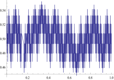
Figure 1: The graph of the values of the Jacobian $J^{12}$ when $\cos(2\,\theta)=0.12$ and $\beta=5.6$. The transition value of $\beta$ is equal to $2.341$. Above the points on the interval are associated with points in $\{1,2\}^{\mathbb{N}}$ using the binary expansion with symbols $1$ and $2$ (by this we mean: on the binary expansion we associate $0$ to $1$, and, $1$ to $2$). We considered strings with $12$ symbols $k_{0},k_{1},...,k_{11}\in\,\{1,2\}$.

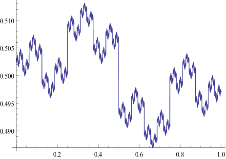
Figure 2: The graph of the values of the Jacobian $J^{12}$ when $\cos(2\,\theta)=0.12$ and $\beta=0.8$. The transition value of $\beta$ is equal to $2.341$. Above the points on the interval are associated with points in $\{1,2\}^{\mathbb{N}}$ using the binary expansion with symbols $1$ and $2$ (by this we mean: on the binary expansion we associate $0$ to $1$, and, $1$ to $2$). We considered strings with $12$ symbols $k_{0},k_{1},...,k_{11}\in\,\{1,2\}$.

Proposition 19.

The image of $J$ is a Cantor set, if and only if, $0<\gamma<\alpha(1-2\alpha)$. In the other case it is an interval. The transition value for $\beta$ where $\gamma=\alpha(1-2\alpha)$ corresponds to the value

$$\beta=\frac{1}{2}\log(\frac{4}{\cos^{2}(2\,\theta)}-1).$$

Proof.

As $f_{0}$ and $f_{1}$ are contractions on $I=[1-R,R]$ (in a suitable metric) the image of $J$ is a regular Cantor set or an interval. We can say exactly when such alternative occurs. If $f_{0}(I)$ and $f_{1}(I)$ are disjoint the attractor will be a Cantor set with Hausdorff dimension strictly between $0$ and $1$. If $f_{0}(I)\cup f_{1}(I)=I$ the attractor is all the interval $I$.

Observe that $f_{0}(I)=[1-R,f_{0}(1-R)]$ and $f_{1}(I)=[f_{1}(1-R),R]$. In this way, $f_{0}(I)$ and $f_{1}(I)$ are disjoint, if and only if, $f_{0}(1-R)<f_{1}(1-R)$. As $f_{0}(1-R)=\alpha+\frac{\gamma}{1-R}$ and $f_{1}(1-R)=1-\alpha-\frac{\gamma}{1-R}$ we have

$$f_{0}(1-R)<f_{1}(1-R)\iff\alpha+\frac{\gamma}{1-R}<1-\alpha-\frac{\gamma}{1-R}\iff$$

$$\frac{2\gamma}{1-R}<1-2\alpha\iff 1-R>\frac{2\gamma}{1-2\alpha}\iff R<1-\frac{2\gamma}{1-2\alpha}.$$

The solutions of $x^{2}-(1-\alpha)x+\gamma=0$ are $\tilde{R}$ and $R$. As $\frac{2\gamma}{1-2\alpha}<\frac{2\gamma}{4\gamma}=1/2$ we get $1-\frac{2\gamma}{1-2\alpha}>1/2>\tilde{R}$. It follows that

$$R<1-\frac{2\gamma}{1-2\alpha}\iff(1-\frac{2\gamma}{1-2\alpha})^{2}-(1-\alpha)(1-\frac{2\gamma}{1-2\alpha})+\gamma>0.$$

Therefore

$$f_{0}(1-R)<f_{1}(1-R)\iff(1-\frac{2\gamma}{1-2\alpha})^{2}-(1-\alpha)(1-\frac{2\gamma}{1-2\alpha})+\gamma>0$$

$$\iff-4\gamma(1-2\alpha)+4\gamma^{2}+\alpha(1-2\alpha)^{2}+2\gamma(1-2\alpha)-2\alpha\gamma(1-2\alpha)+\gamma(1-2\alpha)^{2}>0.$$

The above condition can be expressed as

$$0<4\gamma^{2}-(1-2\alpha)(1+4\alpha)\gamma+\alpha(1-2\alpha)^{2}=(4\gamma+2\alpha-1)(\gamma-\alpha(1-2\alpha)).$$

As $4\gamma+2\alpha-1<0$, this condition is equivalent to $\gamma-\alpha(1-2\alpha)<0$.

Therefore, the conclusion is that the attractor is a regular Cantor set, if and only if,

$$0<\gamma<\alpha(1-2\alpha).$$

From definition of $\alpha$ and $\gamma$ we have $\gamma=\frac{1}{4}\,(1-2\alpha)\cos^{2}(2\,\theta)$. Then the inequality $0<\gamma<\alpha(1-2\alpha)$ is equivalent to $\frac{\cos^{2}(2\,\theta)}{4}<\alpha$. As $\alpha=\frac{\Phi_{\beta}}{2}=\frac{1}{e^{2\,\beta}+1}$ we finally get

$$\frac{\cos^{2}(2\,\theta)}{4}<\frac{1}{e^{2\,\beta}+1}\iff\beta<\frac{1}{2}\log(\frac{4}{\cos^{2}(2\,\theta)}-1).$$

The final conclusion is that the image of $J$ is a regular Cantor set, if and only if,

$$\beta<\frac{1}{2}\log(\frac{4}{\cos^{2}(2\,\theta)}-1).$$

When $\beta$ is larger we get that the image of $J$ is an interval.

∎

As the probability $\mu_{\beta}$ is mixing (because the potential is Hölder) in particular we have that for any cylinders $A=[a_{1},...,a_{k}]$ and $B=[b_{1},...,b_{l}]$:

$$\lim_{n\to\infty}\mu(A\cap\sigma^{-n}B)=\mu(A)\mu(B).$$

This means

$$\lim_{n\to\infty}\sum_{j_{1},...,j_{n}}\mu_{\beta}(a_{1},...,a_{k},j_{1},...,j_{n},b_{1},...,b_{l})=\mu_{\beta}(a_{1},...,a_{k})\mu_{\beta}(b_{1},...,b_{l}).$$ (8)

One can show the following precise result concerning the speed of convergence (see [3] for the computations):

$$\lim_{n\to\infty} \sum_{j_{1},...,j_{n}}\mu_{\beta}(a_{1},a_{2},a_{3},...,a_{k},j_{1},...,j_{n},b_{1},...,b_{l})$$

$$=\bigg{[}\frac{1}{2}\bigg{(}1+\frac{\beta_{a_{1}}}{\beta_{a_{2}}}(-1+\Phi_{\beta})\bigg{)}\mu_{\beta}(a_{2},...,a_{k})\,+$$

$$\hskip 14.22636pt\sum_{j_{1},...,j_{n}}\frac{\beta_{a_{1}}}{2}(-1+\Phi_{\beta})\bigg{(}\frac{-1}{2\beta_{a_{2}}}+\frac{\beta_{a_{2}}}{2}\bigg{)}\mu_{\beta}(a_{3},...,a_{k})\bigg{]}\mu_{\beta}(b_{1},...,b_{l})$$

$$=\mu_{\beta}(a_{1},a_{2},...,a_{k})\mu_{\beta}(b_{1},...,b_{l}).$$

5 LDP

In this section we will present some results which are similar but more complex that the ones in section 5 in [19].

In this section we will prove Theorem 4.

Definition 20.

For $x=(x_{1},x_{2},\cdots)\in\Omega=\{1,2\}^{\mathbb{N}}$ and $A:\Omega\to\mathbb{R}$, we define the $n$-Birkhoff sum for $A$ and $x$ as

$$S_{n}(A,x):=\sum\limits_{j=0}^{n-1}A(\sigma^{j}(x))=A(x)+A(\sigma(x))+\cdots+A(\sigma^{n-1}(x)).$$

Definition 21.

Suppose $A:\Omega\to\mathbb{R}$ is a Hölder function. We define for each $t\in\mathbb{R},$

$$Q_{n}(t):=\int e^{t\,S_{n}(A,x)}d\mu_{\beta}(x).$$

In the case $A$ depends just on the first coordinate we get

$$Q_{n}(t)=\sum_{x_{0}}\,\sum_{x_{1}}\,...\sum_{x_{n}}e^{t\,(A(x_{0})+A(x_{1})+...+A(x_{n}))}\,\mu_{\beta}(x_{0},x_{1},...x_{n}).$$

The free energy on time $t$ is

$$c(t):=\lim_{n\to\infty}\frac{1}{n}\,\,\log\int e^{t\,S_{n}(A,z)}d\mu_{\beta}(z)=\lim_{n\to\infty}\frac{1}{n}\,\,\log Q_{n}(t),$$

for each $t\in\mathbb{R}$.

Remember that

$$\delta(t)=\sum_{j}e^{t\,\,A(j)}\,\,\,\text{ and }\,\,\,\alpha(t)=\sum_{j}\beta_{j}\,e^{t\,\,A(j)}.$$

Remark 22.

Note that $|\alpha(t)|<|\delta(t)|$, because $|\beta_{j}|\leq 1$ and $\beta_{1}=-\beta_{2}$. Moreover, note that $\delta(t)>0$.

We will show that for any $t\in\mathbb{R}$,

$$c(t)=\log\left(\frac{\Phi_{\beta}\delta(t)+\sqrt{\Phi_{\beta}^{2}\delta(t)^{2}+4(-1+\Phi_{\beta})(\alpha(t)^{2}-\delta(t)^{2})}}{4}\right).$$

The function $c(t)$ is differentiable on $t$.

Example 23.

We will estimate $Q_{3}(t)$. From Theorem 11 we get

$$\mu_{\beta}(j_{0},j_{1},j_{2},j_{3})= \frac{\mu_{\beta}(j_{1},j_{2},j_{3})}{2}+\frac{(-1+\Phi_{\beta})\beta_{j_{0}}\beta_{j_{1}}}{4}\mu_{\beta}(j_{2},j_{3})\,+$$

$$\frac{(-1+\Phi_{\beta})^{2}\beta_{j_{0}}\beta_{j_{2}}}{16}+\frac{(-1+\Phi_{\beta})^{3}\beta_{j_{0}}\beta_{j_{3}}}{16},$$

therefore,

$$Q_{3}(t) =\sum_{j_{0}}\,\sum_{j_{1}}\,\sum_{j_{2}}\sum_{j_{3}}e^{t\,(A(j_{0})+A(j_{1})+A(j_{2})+A(j_{3}))}\,\mu_{\beta}(j_{0},j_{1},j_{2},j_{3})$$

$$=\bigg{[}\frac{1}{2}\sum_{j_{0}}\,e^{t\,A(j_{0})}\,\bigg{]}\,\sum_{j_{1}}\,\sum_{j_{2}}\sum_{j_{3}}\,e^{t\,(A(j_{1})+A(j_{2})+A(j_{3}))}\,\mu_{\beta}(j_{1},j_{2},j_{3})$$

$$+\frac{(-1+\Phi_{\beta})}{4}\bigg{[}\sum_{j_{0}}e^{t\,A(j_{0})}\beta_{j_{0}}\bigg{]}\,\bigg{[}\sum_{j_{1}}e^{t\,A(j_{1})}\beta_{j_{1}}\bigg{]}\,\sum_{j_{2},j_{3}}e^{t\,(A(j_{2})+A(j_{3}))}\mu_{\beta}(j_{2},j_{3})$$

$$+\frac{(-1+\Phi_{\beta})^{2}}{16}\sum_{j_{0}}\,\sum_{j_{1}}\,\sum_{j_{2}}\sum_{j_{3}}e^{t\,(A(j_{0})+A(j_{1})+A(j_{2}))+A(j_{3})}\beta_{j_{0}}\beta_{j_{2}}$$

$$+\frac{(-1+\Phi_{\beta})^{3}}{16}\sum_{j_{0}}\,\sum_{j_{1}}\,\sum_{j_{2}}\sum_{j_{3}}e^{t\,(A(j_{0})+A(j_{1})+A(j_{2}))+A(j_{3}))}\beta_{j_{0}}\beta_{j_{3}}$$

$$=\frac{1}{2}\delta(t)Q_{2}(t)+\frac{(-1+\Phi_{\beta})}{4}\alpha(t)^{2}Q_{1}(t)+\frac{\Phi_{\beta}(-1+\Phi_{\beta})^{2}}{16}\alpha^{2}(t)\delta^{2}(t).$$

In the general case we get:

Theorem 24.

For all $n\in\mathbb{N}$ and $t\in\mathbb{R}$

$$Q_{n}(t)=\left[\begin{array}[]{l}\frac{1}{2}\delta(t)\,Q_{n-1}(t)+\frac{(-1+\Phi_{\beta})}{4}\alpha(t)^{2}\,Q_{n-2}(t)+\frac{(-1+\Phi_{\beta})^{2}}{8}\delta(t)\,\alpha(t)^{2}\,Q_{n-3}(t)\\ \\ \,\,+\frac{(-1+\Phi_{\beta})^{3}}{16}\delta(t)^{2}\,\alpha(t)^{2}\,\,Q_{n-4}(t)+\frac{(-1+\Phi_{\beta})^{4}}{32}\delta(t)^{3}\,\alpha(t)^{2}\,\,Q_{n-5}(t)+...+\\ \\ +\frac{(-1+\Phi_{\beta})^{n-3}}{2^{n-2}}\,\delta(t)^{n-4}\,\alpha(t)^{2}\,\,Q_{2}(t)+\frac{(-1+\Phi_{\beta})^{n-2}}{2^{n-1}}\,\delta(t)^{n-3}\,\alpha(t)^{2}\,\,Q_{1}(t)\\ \\ +\frac{\Phi_{\beta}(-1+\Phi_{\beta})^{n-1}}{2^{n+1}}\alpha^{2}(t)\delta^{n-2}(t).\end{array}\right].$$ (9)

For the proof see Appendix (Theorem 38)

Proposition 25.

$$Q_{n+2}(t)=(-1+\Phi_{\beta})\frac{\alpha(t)^{2}-\delta(t)^{2}}{4}\,Q_{n}(t)+\frac{\Phi_{\beta}}{2}\delta(t)\,Q_{n+1}(t).$$

For the proof see Appendix (Theorem 39)

The equation presented in Proposition 25 (positive temperature) is more complex when compared with the analogous one (Proposition 5.2) in [19] (zero temperature). Note that at zero temperature $\beta\to\infty$ and $\Phi_{\beta}\to 0$. At zero temperature the last term above disappears. In the present case $\Phi_{\beta}>0$, and we need a recurrence relation.

Note that for fixed $t$ and $\beta$ the expressions $(-1+\Phi_{\beta})\frac{\alpha(t)^{2}-\delta(t)^{2}}{4}$ and $\frac{\Phi_{\beta}}{2}\delta(t)$ do not depend on $n$. For each $t$ we get a second order recurrence relation which will solved by using a result we get from [25]:

Theorem 26.

Given the real numbers $s_{1}$ and $s_{2}$ suppose that $r_{1},r_{2}$ are the roots of the equation $x^{2}-s_{1}\,x-s_{2}=0$. If $r_{1}\neq r_{2}$, then, any solution of the recurrence equation

$$a_{n}=s_{1}a_{n-1}+s_{2}a_{n-2}$$

is of the form

$$a_{n}=c_{1}r_{1}^{n}+c_{2}r_{2}^{n},$$

where $c_{1},c_{2}$ are constants.

Proof of Theorem 4: Let’s check that the recurrence relation presented in Proposition 25 satisfies the hypothesis of theorem 26. The roots of

$$x^{2}-\frac{\Phi_{\beta}}{2}\,\delta(t)\,x-(-1+\Phi_{\beta})\frac{\alpha(t)^{2}\,-\,\delta(t)^{2}}{4}$$

are

$$r_{1}=r_{1}(t)= \frac{\frac{\Phi_{\beta}}{2}\delta(t)+\sqrt{\frac{\Phi_{\beta}^{2}}{4}\delta(t)^{2}+4(-1+\Phi_{\beta})\frac{\alpha(t)^{2}-\delta(t)^{2}}{4}}}{2}$$

$$=\frac{\Phi_{\beta}\delta(t)+\sqrt{\Phi_{\beta}^{2}\delta(t)^{2}+4(-1+\Phi_{\beta})(\alpha(t)^{2}-\delta(t)^{2})}}{4}$$

and

$$r_{2}=r_{2}(t)= \frac{\frac{\Phi_{\beta}}{2}\delta(t)-\sqrt{\frac{\Phi_{\beta}^{2}}{4}\delta(t)^{2}+4(-1+\Phi_{\beta})\frac{\alpha(t)^{2}-\delta(t)^{2}}{4}}}{2}$$

$$=\frac{\Phi_{\beta}\delta(t)-\sqrt{\Phi_{\beta}^{2}\delta(t)^{2}+4(-1+\Phi_{\beta})(\alpha(t)^{2}-\delta(t)^{2})}}{4}.$$

By Remark 22 it follows that $\Phi_{\beta}\delta(t)>0$ and moreover $4\,(-1+\Phi_{\beta})\,(\alpha(t)^{2}-\delta(t)^{2})>0$, because $\Phi_{\beta}\in(0,1)$. In this case, $r_{1}\neq r_{2}$. Moreover, $r_{1}>-r_{2}>0$. Indeed,

$$\sqrt{\Phi_{\beta}^{2}\delta(t)^{2}+4(-1+\Phi_{\beta})(\alpha(t)^{2}-\delta(t)^{2})}>\sqrt{\Phi_{\beta}^{2}\delta(t)^{2}}=\Phi_{\beta}\delta(t)>0.$$

Therefore,

$$Q_{n}(t)=c_{1}(t)r_{1}(t)^{n}+c_{2}(t)r_{2}(t)^{n}$$

with $r_{1}>-r_{2}>0$. It follows that, for any $t$,

$$c(t) =\lim_{n\to\infty}\frac{1}{n}\log Q_{n}(t)=\log r_{1}(t)$$

$$=\log\left(\frac{\Phi_{\beta}\delta(t)+\sqrt{\Phi_{\beta}^{2}\delta(t)^{2}+4(-1+\Phi_{\beta})(\alpha(t)^{2}-\delta(t)^{2})}}{4}\right).$$

∎

6 Some results on zero temperature

In this section we will complement some results obtained in [19]. We denote by $\mu$ the zero temperature quantum spin probability on $\{1,2\}^{\mathbb{N}}$ as described in [19] which is ergodic but not mixing. We want to prove Theorem 5. Initially we remember some definitions and results from [19].

We denote in this section $\beta_{1}=\sin(2\,\theta)$, $\beta_{2}=-\beta_{1}$, $\gamma=\frac{1}{4}\bigg{(}1-\beta_{1}^{2}\bigg{)}=\mu(1,1),$

$$a(k_{0},k_{1})=\frac{1}{2}\bigg{(}1-\frac{\beta_{k_{0}}}{\beta_{k_{1}}}\bigg{)}$$

and

$$b(k_{0},k_{1})=\frac{1}{4}\beta_{k_{0}}\bigg{(}\frac{1}{\beta_{k_{1}}}-\beta_{k_{1}}\bigg{)}.$$

At zero temperature we get

a) if $k_{0}=k_{1}$, then $a(k_{0},k_{1})=0$ and $0<b(k_{0},k_{1})=\gamma=\frac{1}{4}(1-\beta_{1}^{2})<\frac{1}{4}$

b) if $k_{0}\neq k_{1}$, then $a(k_{0},k_{1})=1$ and $-\frac{1}{4}<b(k_{0},k_{1})=-\gamma=\frac{1}{4}(\beta_{1}^{2}-1)<0$

Using $a$ and $b$ the measure $\mu$ can be computed recursively in finite cylinders by $\mu(\{1,2\}^{\mathbb{N}})=1$, $\mu(1)=\mu(2)=1/2$ and, for $n\geq 1$,

$$\mu(k_{0},k_{1},k_{2},...,k_{n})=a(k_{0},k_{1})\mu(k_{1},k_{2},k_{3},...,k_{n})+b(k_{0},k_{1})\mu(k_{2},k_{3},...,k_{n}),$$

which can be rewritten as

$$\frac{\mu(k_{0},k_{1},k_{2},...,k_{n})}{\mu(k_{1},k_{2},...,k_{n})}=a(k_{0},k_{1})+b(k_{0},k_{1})\frac{1}{\frac{\mu(k_{1},k_{2},k_{3},...,k_{n})}{\mu(k_{2},k_{3},...,k_{n})}}.$$ (10)

The Jacobian $J$ of the invariant probability $\mu$ is given by

$$J(k_{0},k_{1},k_{2},...,k_{n},...)=\lim_{n\to\infty}\frac{\mu(k_{0},k_{1},k_{2},...,k_{n})}{\mu(k_{1},k_{2},...,k_{n})}$$

which exists $\mu$ almost everywhere and satisfies the lemma below (see [19]).

Lemma 27.

$$J(k_{0},k_{1},k_{2},...)=a(k_{0},k_{1})+b(k_{0},k_{1})\frac{1}{J(k_{1},k_{2},k_{3},...)}$$ (11)

and

$$J(k_{0} ,k_{1},k_{2},...)=\lim_{n}\left[a(k_{0},k_{1})+b(k_{0},k_{1})\,\frac{1}{a(k_{1},k_{2})+b(k_{1},k_{2})\frac{1}{...a(k_{n-1},k_{n})+b(k_{n-1},k_{n})\frac{1}{1/2}}}\right],$$

if the limit exists.

In this sense ${J}$ has an expression in continued fraction (according to [19]). The following result is mentioned in [19]. Below we will provide a complete proof.

Theorem 28.

At zero temperature the Jacobian of $\mu$ assumes just two values $p$ and $1-p$ almost everywhere, where $p=\frac{1+\beta_{1}}{2}$.

From now on we present some new material which was not discussed in [19].

Let $A$ be the set of points $\theta\in\{0,1\}^{\mathbb{N}}$ such that $J(\theta)=p$ and $B$ be the set of points $\theta\in\{0,1\}^{\mathbb{N}}$ such that $J(\theta)=1-p$. The sets $A$ and $B$ are Borel sets. Indeed, given positive integers $m$ and $n_{0}$, the set $X(m,n_{0})$ of the points $\theta=(\theta_{0},\theta_{1},\dots)\in\{1,2\}^{\mathbb{N}}$, such that, for some $n\geq n_{0}$, $|\frac{\mu(k_{0},k_{1},k_{2},...,k_{n})}{\mu(k_{1},k_{2},...,k_{n})}-p|>1/m$ is a union of cylinder sets, therefore an open set. From this we get $A=\cap_{m\in{\mathbb{N}^{*}}}(\{1,2\}^{\mathbb{N}}\setminus\cap_{n_{0}\in{\mathbb{N}^{*}}}X(m,n_{0}))$ is a Borel set. The same argument shows that $B$ is a Borel set.

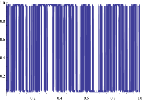
Figure 3: The graph of the values of the Jacobian $J^{12}$ at zero temperature when $\cos(2\,\theta)=0.96$. The maximum and minimum values are $p$ and $(1-p)$. Above the points on the interval are associated with points in $\{1,2\}^{\mathbb{N}}$ using the binary expansion with symbols $1$ and $2$. (by this we mean: on the binary expansion we associate $0$ to $1$, and, $1$ to $2$). We considered strings with $12$ symbols $k_{0},k_{1},...,k_{11}\in\,\{1,2\}$.

The next proposition assures that when comparing $\theta$ and $\sigma(\theta)$ we have the alternative: there are a change of the set (where they are), or, there are a change of the first coordinate.

Proposition 29.

Given $\theta=(k_{0},k_{1},k_{2},...)\in A\cup B$, the points $\theta$ and $\sigma(\theta)$ belong to the same set (both in $A$ or both in $B$), iff, $k_{0}\neq k_{1}$.

Proof As $\gamma/p=1-p,\,1-\gamma/p=p,\,\gamma/(1-p)=p$ and $1-\gamma/(1-p)=1-p$, using the equation (11), we get:

• $\text{ if }\theta=(k_{0},k_{1},k_{2},...)\in A\text{ begins with }1,\text{ then }\,2\theta\in A,\,1\theta\in B,$

• $\text{ if }\theta=(k_{0},k_{1},k_{2},...)\in A\text{ begins with }2,\text{ then }\,1\theta\in A,\,2\theta\in B,$

• $\text{ if }\tilde{\theta}=(k_{0},k_{1},k_{2},...)\in B\text{ begins with }1,\text{ then }\,1\tilde{\theta}\in A,\,2\tilde{\theta}\in B,$

• $\text{if }\tilde{\theta}=(k_{0},k_{1},k_{2},...)\in B\text{ begins with }2,\text{ then}\,2\tilde{\theta}\in A,\,1\tilde{\theta}\in B.$

∎

Theorem 30.

The entropy of the quantum spin probability at zero temperature is

$$-p\log p-(1-p)\log(1-p).$$

Proof: The entropy of $\mu$ is given by $h(\mu)=-\int\log Jd\mu=-\log(p)\mu(A)-\log(1-p)\mu(B).$ It remains to prove that $\mu(A)=p$ and $\mu(B)=1-p$.

We have $\sigma(A)=\sigma(B)=A\cup B=\{1,2\}^{\mathbb{N}}$ almost everywhere and $\sigma|A$ and $\sigma|B$ are injective, then, since the Jacobian of $\mu$ in $A$ is $p$ and in $B$ is $1-p$, for any measurable sets $X\subset A$, $Y\subset B$, we get

$$\mu(\sigma(X))=\mu(X)/p\hskip 28.45274pt\,\text{and}\hskip 28.45274pt\,\mu(\sigma(Y))=\mu(Y)/(1-p).$$ (12)

Particularly,

$$1=\mu(A\cup B)=\mu(\sigma(A))=\mu(A)/p.$$ (13)

This shows that $\mu(A)=p$ and consequently $\mu(B)=1-p$.

∎

We will present later an ergodic conjugacy of $(\sigma,\mu)$ with another dynamical system which is “in some way” related with $(\sigma,m_{p})$ where $m_{p}$ is the independent Bernoulli probability $(p,1-p)$.

Before we start the proof of Theorem 28 we need an auxiliary result. Part of it can be found in the arXiv version 1505.01305 of [19].

Lemma 31.

For any $n\geq 1$ and $k_{1},...,k_{n}\in\{1,2\}$ we have

$$\frac{\mu(1,2,2,1,1,k_{1},...,k_{n})}{\mu(2,2,1,1,k_{1},...,k_{n})}=\frac{\mu(1,k_{1},...,k_{n})}{\mu(k_{1},...,k_{n})}$$

and

$$\frac{\mu(1,1,2,2,1,k_{1},...,k_{n})}{\mu(1,2,2,1,k_{1},...,k_{n})}=\frac{\mu(1,k_{1},...,k_{n})}{\mu(k_{1},...,k_{n})}.$$

Particularly, $J$ is not defined in $(1,1,2,2)^{\infty}=(1,1,2,2,1,1,2,2,1,...).$ A similar result is true if we permute the symbols $1$ and $2$.

Proof.

From (10) we get

$$\frac{\mu(1,2,2,1,1,k_{1},...,k_{n})}{\mu(2,2,1,1,k_{1},...,k_{n})}=1-\gamma\frac{1}{0+\gamma\frac{1}{1-\gamma\frac{1}{0+\gamma\frac{1}{\frac{\mu(1,k_{1},...,k_{n})}{\mu(k_{1},...,k_{n})}}}}}=\frac{\mu(1,k_{1},...,k_{n})}{\mu(k_{1},...,k_{n})}$$

and

$$\frac{\mu(1,1,2,2,1,k_{1},...,k_{n})}{\mu(1,2,2,1,k_{1},...,k_{n})}=\gamma\frac{1}{1-\gamma\frac{1}{\gamma\frac{1}{1-\gamma\frac{1}{\frac{\mu(1,k_{1},...,k_{n})}{\mu(k_{1},...,k_{n})}}}}}=\frac{\mu(1,k_{1},...,k_{n})}{\mu(k_{1},...,k_{n})}.$$

Particularly,

$$\frac{\mu(1,1,2,2,...,1,1,2,2,1,1)}{\mu(1,2,2,...,1,1,2,2,1,1)}=\frac{\mu(1,1)}{\mu(1)}=\frac{\gamma}{2}$$

and

$$\frac{\mu(1,1,2,2,...,1,1,2,2,1)}{\mu(1,2,2,...,1,1,2,2,1)}=\mu(1)=\frac{1}{2}.$$

This proves that $J$ is not defined in $(1,1,2,2)^{\infty}$.

These computations can be applying permuting the symbols $1$ and $2$. ∎

A slightly different version of the next proof can be found in the arXiv version of [19].

Proof of Theorem 28:

The value of $J$ does not change if we permute $1$ and $2$ in the sequence $(k_{0},k_{1},...)\in\{1,2\}^{\mathbb{N}}$. For example

$$J(1,1,1,2,2,1,...)=J(2,2,2,1,1,2,...)$$

(if the limit exists). Therefore, we will introduce another code. For each given sequence $k\in\{1,2\}^{\mathbb{N}}$, $k=(k_{0},k_{1},k_{2},...)$ we associate a new sequence $m=m(k)=(m_{0},m_{1},m_{2},..)\in\{a,b\}^{\mathbb{N}}$ by the rule: $m_{i}=a$ if $k_{i}=k_{i+1}$ and $m_{i}=b$ if $k_{i}\neq k_{i+1}$. So, we are looking if there is a change, or not, in the string $k$ by using the rules $\underbrace{11}_{a}$ ,  $\underbrace{22}_{a}$ , $\underbrace{12}_{b}$ ,  $\underbrace{21}_{b}$.

For example, given a sequence $k$ of the form

$$k=(1,2,1,1,2,2,...),$$

then, we associate $m=(b,b,a,b,..).$ Clearly, we can consider $J$ defined over $\{a,b\}^{\mathbb{N}}$, from $J(m(k)):=J(k)$.

It can be checked that:

$$J(a,a,m_{3},..) =J(m_{3},m_{4},..)$$

$$J(a,b,m_{3},..) =\frac{1}{\gamma^{-1}-\frac{1}{J(m_{3},m_{4},..)}}$$

$$J(b,a,m_{3},..) =1-J(m_{3},m_{4},..)$$

$$J(b,b,m_{3},..) =1-\frac{1}{\gamma^{-1}-\frac{1}{J(m_{3},m_{4},..)}}.$$

From Proposition 4.2 in [19] we obtain that for $m=(m_{1},...,m_{k},a,a,a...)$, $J(m)$ is not defined. For the other sequences, the finite strings with $(aa)^{n}$, $n\in\mathbb{N}$, can be deleted (when $J$ converges). That is,

$$J(m_{0},m_{1},...,m_{j},a,a,m_{j+2},...)=J(m_{0},m_{1},...,m_{j},m_{j+2},...).$$

Consider the letters of $m$ arranged in blocks of length 2,

$$m=([m_{1},m_{2}],[m_{3},m_{4}],[m_{5},m_{6}],...).$$

As we are interested in the value of $J$, we can assume that no blocks have the form $[a,a]$ (we can delete them) and also that no blocks have the form $[b,b]$, because we can replace this one for the pair of blocks $[b,a],[a,b]$.

From now on it is natural to consider one level up of symbolic representation. We get a new code introducing a new dictionary where we associate $\alpha=[a,b]=a,b$ and $\beta=[b,a]=b,a$. In this way, for $m=(m_{0},m_{1},m_{2},...)=([m_{0},m_{1}],[m_{2},m_{3}],...)$ we associate $w=(w_{0},w_{1},w_{2},...)$, where $w_{i}=\alpha$, if $[m_{2i},m_{2i+1}]=[a,b]$, and $w_{i}=\beta$, if $[m_{2i},m_{2i+1}]=[b,a]$.

We need to study the possible values of $J$ over $\{\alpha,\beta\}^{\mathbb{N}}$. First we remark that the strings $\alpha,\alpha$ and $\beta,\beta$ in $w$ correspond to the strings $a,b,a,b$ and $b,a,b,a$ in $m$, which can be deleted without changes of the value of $J$. Indeed, as a consequence of Lemma 31 we get

$$J(a,b,a,b,m_{5},m_{6},...)=J(b,a,b,a,m_{5},m_{6},...)=J(m_{5},m_{6},m_{7},...).$$

In the finite fraction expansion of odd order of $k$ (which is associated to a certain string $m$ of even order and so to a string $w$) we can delete parts (in the $\alpha,\beta$ dictionary expansion) in such a way that we end up with the estimation of $J$ in a string $w$ of one of the kinds: $(\alpha\,\beta)^{n}$, $(\alpha\,\beta)^{n}\alpha$, $(\beta\,\alpha)^{n}$ or $(\beta\,\alpha)^{n}\beta$.

From now on, we use the above conclusion in order to determine what are the possible values of $J$. Consider the transformation

$$x\,\to\,f_{1}(x)=1-\frac{1}{\gamma^{-1}-\frac{1}{x}}.$$

The string $\beta\alpha$ means $baab$, which corresponds to

$$J(w_{1},w_{2},w_{3},..)=1-\frac{1}{\gamma^{-1}-\frac{1}{J(w_{3},w_{4},..)}}.$$

Note that if the expansion $J(w_{3},w_{4},..)$ exists for the string $(w_{3},w_{4},..)$, then it also exists the one for $J(w_{1},w_{2},w_{3},..)$. In this way $f_{1}(J(w_{3},w_{4},..))=J(w_{1},w_{2},w_{3},..).$

Consider now $f_{2}$ defined by

$$x\,\to\,f_{2}(x)=\frac{1}{\gamma^{-1}-\frac{1}{1-x}}\,\,.$$

The string $\alpha\,\beta$ means $abba$, that is, it corresponds to

$$J(w_{1},w_{2},w_{3},..)=\frac{1}{\gamma^{-1}-\frac{1}{1-J(w_{3},w_{4},..)}}.$$

In this way $f_{2}(J(w_{3},w_{4},..))=J(w_{1},w_{2},w_{3},..).$

Note that the fixed points for both functions $f_{1}(x)=1-\frac{1}{\gamma^{-1}-\frac{1}{x}}$ and $f_{2}(x)=\frac{1}{\gamma^{-1}-\frac{1}{1-x}}$ are the same: $p=\frac{1+\beta_{1}}{2}$ and $1-p=\frac{1-\beta_{1}}{2}$ (it’s helpful to observe also that $\gamma=p(1-p)$ ). Furthermore, the interval $[1-p,p]$ is invariant by $f_{1}$ and also by $f_{2}$. The point $p$ is a global attractor for $f_{1}$ in $(1-p,p]$ and $1-p$ is a global attractor for $f_{2}$ in $[1-p,p)$.

As we have seen in Lemma 27 it is natural to truncate $J(k_{0},k_{1},k_{2},\dots)$ (at level $r$ for instance) by taking in the last position $r$, in the expansion of $J$, the value $1/2$. As $1/2\in[1-p,p]$ (in fact is its center), and the interval $[1-p,p]$ is left invariant by the diffeomorphisms $g_{a}(x)=\frac{\gamma}{x}$ and $g_{b}(x)=1-\frac{\gamma}{x}$, when the limit exists the successive truncations should converge to $p$ or to $1-p$.

Then, the only possible (convergent) values attained by the continuous fraction expansion of $J$ are $p$ or $1-p$.

∎

Proposition 32.

There exists a map

$$h:(\{1,2\}^{\mathbb{N}},\sigma,\mu)\to(\{0,1\}^{\mathbb{N}},\sigma,\mu_{p}),$$

which is probability preserving, where $\mu_{p}$ is the Bernoulli independent probability associated to $(p,1-p)$. However, $(\{1,2\}^{\mathbb{N}},\sigma,\mu)$ and $(\{0,1\}^{\mathbb{N}},\sigma,\mu_{p})$ are not ergodically equivalent.

Proof.

We set $h(\theta)=(c_{0},c_{1},c_{2},...)$, where $c_{j}=0$, if $\sigma^{j}(\theta)\in A$, and $c_{j}=1$, if $\sigma^{j}(\theta)\in B$. This map $h$ is defined for $\mu$-almost every point of $\{1,2\}^{\mathbb{N}}$ and we may to extend $h$ to $\{1,2\}^{\mathbb{N}}\setminus(A\cup B)$ as $(0,0,0,\dots)$. $h:(\{1,2\}^{\mathbb{N}},\mu)\to(\{0,1\}^{\mathbb{N}},\mu_{p})$, where $\mu_{p}$ is the Bernoulli independent probability associated to $p$ for $0$, and $1-p$ for $1$. Clearly $h\circ\sigma=\sigma\circ h$.

By the above properties of $A$ and $B$, we have the following expression for $h$: if $\alpha=(a_{0},a_{1},a_{2},a_{3},\dots)\in\{1,2\}^{\mathbb{N}}$, let $c_{0}=\chi_{B}(\alpha)$; then $h(\alpha)=(c_{0},c_{0}+a_{0}+a_{1}+1\pmod{2},c_{0}+a_{0}+a_{2}\pmod{2},c_{0}+a_{0}+a_{3}+1\pmod{2},\dots).$

In order to show that $h$ is a measurable map we observe that for any cylinder set $[c_{0},...,c_{n}]\subset\{0,1\}^{\mathbb{N}}$ we have

$$h^{-1}([c_{0},...,c_{n}])=h^{-1}([c_{0}])\cap h^{-1}(\sigma^{-1}[c_{1}])\cap...\cap h^{-1}(\sigma^{-n}([c_{n}]))$$

$$=h^{-1}([c_{0}])\cap\sigma^{-1}(h^{-1}([c_{1}])\cap...\cap\sigma^{-n}(h^{-1}([c_{n}])),$$

which is a Borel set because, for each $i\in\{0,...,n\}$, $h^{-1}([c_{i}])$ is $A$ or $B$.

Now we will show that $\mu_{p}([c_{0},...,c_{n}])=\mu(h^{-1}([c_{0},...,c_{n}]))$, for any cylinder set $[c_{0},c_{1},...,c_{n}]\subset\{0,1\}^{\mathbb{N}}$. The proof is by induction. For cylinders of length 1 we have,

$$\mu_{p}([0])=p\stackrel{{\scriptstyle(\ref{muA})}}{{=}}\mu(A)=\mu(h^{-1}([0]))\,\,\,and\,\,\,\mu_{p}([1])=1-p=\mu(B)=\mu(h^{-1}([1])).$$

From now on we suppose that for any cylinder of length $n$ the claim is satisfied. Given a cylinder of length $n+1$ in the form $[0,c_{1},...,c_{n},c_{n+1}]$ we have

$$h^{-1}([0,c_{1},...,c_{n},c_{n+1}])=h^{-1}([0]\cap\sigma^{-1}([c_{1},...,c_{n}]))=A\cap h^{-1}(\sigma^{-1}([c_{1},...,c_{n}]))$$

$$=A\cap\sigma^{-1}\circ h^{-1}([c_{1},...,c_{n}])),$$

and, from equation (12)

$$\mu(h^{-1}([0,c_{1},...,c_{n},c_{n+1}]))=\mu(A\cap\sigma^{-1}\circ h^{-1}([c_{1},...,c_{n}]))$$

$$\stackrel{{\scriptstyle(\ref{eq2})}}{{=}}\mu(\sigma(A)\cap h^{-1}([c_{1},...,c_{n}])))\cdot p=\mu(h^{-1}([c_{1},...,c_{n}])))\cdot p=\mu_{p}([c_{1},...,c_{n}])\cdot p$$

$$=\mu_{p}([0,c_{1},...,c_{n}]).$$

The same kind of computations can be applied for a cylinder of the form $[1,c_{1},...,c_{n}]$, which concludes the proof of the claim. The Kolmogorov extension theorem can be used to extend the result for any Borel set $X\subset\{0,1\}^{\mathbb{N}}$.

The two systems are not ergodically equivalent because the independent Bernoulli system is mixing.

∎

If $\alpha=(a_{0},a_{1},a_{2},a_{3},\dots)\in\{1,2\}^{\mathbb{N}}$ and $c_{0}:=\chi_{B}(\alpha)$; then $h(\alpha)=(c_{0},c_{0}+a_{0}+a_{1}+1\pmod{2},c_{0}+a_{0}+a_{2}\pmod{2},c_{0}+a_{0}+a_{3}+1\pmod{2},\dots).$ As an example, note that the restriction of $h$ to $A\cap(\{1\}\times\{1,2\}^{{\mathbb{N}}^{*}})$ is given by

$$h(1,a_{1},a_{2},a_{3},a_{4},\dots)=$$

$$(0,a_{1}\pmod{2},1+a_{2}\pmod{2},a_{3}\pmod{2},1+a_{4}\pmod{2},\dots)=$$

$$(0,2-a_{1},a_{2}-1,2-a_{3},a_{4}-1,\dots),$$

and, therefore is an homeomorphism onto its image $\{0\}\times\{0,1\}^{\mathbb{N}^{*}}$, with inverse map given by

$$(h|_{A\cap(\{1\}\times\{1,2\}^{{\mathbb{N}}^{*}})})^{-1}(0,c_{1},c_{2},c_{3},c_{4},\dots)=(1,2-c_{1},c_{2}+1,2-c_{3},c_{4}+1,\dots).$$

Therefore, $h(A\cap(\{1\}\times\{1,2\}^{\mathbb{N}^{*}}))$ is a Borel set. The same kind of argument can be applied for $h(A\cap(\{2\}\times\{1,2\}^{\mathbb{N}^{*}})),h(B\cap(\{1\}\times\{1,2\}^{\mathbb{N}^{*}}))$ and $h(B\cap(\{2\}\times\{1,2\}^{\mathbb{N}^{*}}))$, which proves that $h(A\cup B)$ is a Borel set. The image of $h$ has full measure for $\mu_{p}$, because

$$\mu_{p}(h(A\cup B))=\mu(h^{-1}(h(A\cup B)))\geq\mu(A\cup B)=1.$$

This map $h$ is not an ergodic equivalence between $(\{1,2\}^{\mathbb{N}},\sigma,\mu)$ and $(\{0,1\}^{\mathbb{N}},\sigma,\mu_{p})$. Otherwise, would be essentially a bijection, that is, it will exist subsets of zero measure $X$ of $(\{1,2\}^{\mathbb{N}},\mu)$ and $Y$ of $(\{0,1\}^{\mathbb{N}},\mu_{p})$, such that, $h$ restricted to $\{1,2\}^{\mathbb{N}}\setminus X$ is a bijection with $\{0,1\}^{\mathbb{N}}\setminus Y$. This is not true in this case, because $\theta\in A$, if and only if, $\theta^{*}\in A$, where, if $\theta=(a_{0},a_{1},a_{2},...)\in\{1,2\}^{\mathbb{N}}$, $\theta^{*}:=(3-a_{0},3-a_{1},3-a_{2},...)$. Therefore, $h(\theta)=h(\theta^{*})$, for all $\theta\in\{1,2\}^{\mathbb{N}}$.

As $h(\theta)=h(\theta^{*})$ for all $\theta\in\{1,2\}^{\mathbb{N}}$, we get $h(\{1\}\times\{1,2\}^{{\mathbb{N}}^{*}})=h(\{2\}\times\{1,2\}^{{\mathbb{N}}^{*}})=h(\{1,2\}^{\mathbb{N}})$. On the other hand, $h(\theta)=h(\theta^{\prime})$, if and only if, $\theta^{\prime}=\theta$ or $\theta^{\prime}=\theta^{*}$. Indeed, suppose that the first term of $\theta$ coincides with the first of $\theta^{\prime}$. As $h(\theta)=h(\theta^{\prime})$, $\theta$ belongs to $A$, if and only if, $\theta^{\prime}$ belongs to $A$, and $\sigma(\theta)$ belongs to $A$, if and only if, $\sigma(\theta^{\prime})$ also belongs to a $A$. Therefore, by the properties already discussed for the sets $A$ and $B$, the second terms of $\theta$ e $\theta^{\prime}$ coincide. By exchanging $\theta$ and $\theta^{\prime}$ by $\sigma(\theta)$ and $\sigma(\theta^{\prime})$, we can show by induction (using the equality $h(\sigma(\theta))=h(\sigma(\theta^{\prime}))$) that all terms of $\theta$ and $\theta^{\prime}$ coincide, that is, we get $\theta=\theta^{\prime}$. If the first term of $\theta$ does not coincide with the first of $\theta^{\prime}$, then it coincides with the first term of $\theta^{*}$ and the same argument shows that in this case $\theta^{\prime}=\theta^{*}$.

Proposition 33.

There exists an ergodic equivalence $H$ between the shift acting on $(\{1,2\}^{\mathbb{N}},\mu)$ and a certain transformation $T$ acting in an invariant way on $(\{0,1\}\times\{0,1\}^{\mathbb{N}},\mu_{0}\times\mu_{p})$, where $\mu_{0}$ is the uniform probability on $\{0,1\}$, that is, such that, $\{0\}$ e $\{1\}$ have both measure $1/2$.

Proof: We denote a point of $\{0,1\}\times\{0,1\}^{\mathbb{N}}$ by $(c_{0},(c_{1},c_{2},...,c_{n},...)),$ where $c_{0}\in\{0,1\}$, and $(c_{1},c_{2},...)\in\{0,1\}^{\mathbb{N}}$.

Let $T:(\{0,1\}\times\{0,1\}^{\mathbb{N}}\to\{0,1\}\times\{0,1\}^{\mathbb{N}}$ be the transformation

$$T(c_{0},(c_{1},c_{2}...))=(1-c_{0},(c_{2},c_{3},...))=(1-c_{0},\sigma(c_{1},c_{2},...)).$$

Observe that $T$ preserves the probability $\mu_{0}\times\mu_{p}$ in $\{0,1\}\times\{1,2\}^{\mathbb{N}}$.

The ergodic equivalence $H$ between the two systems $(\{1,2\}^{\mathbb{N}},\sigma,\mu)$ and $(\{0,1\}\times\{0,1\}^{\mathbb{N}},T,\mu_{0}\times\mu_{p})$ is given by $H=u\circ g$ where $g:\{1,2\}^{\mathbb{N}}\to\{0,1\}\times\{0,1\}^{\mathbb{N}}$ satisfies

$$g(a_{0},a_{1},a_{2},...)=(2-a_{0},h(a_{0},a_{1},a_{2},...))$$

and $u:\{0,1\}\times\{0,1\}^{\mathbb{N}}\to\{0,1\}\times\{0,1\}^{\mathbb{N}}$ satisfies

$$u(c_{0},(c_{1},c_{2},c_{3},...))=(c_{0}+c_{1}\pmod{2},(c_{1},c_{2},c_{3},...)).$$

From the previous discussion the transformation $g$ is injective and its image, which is $\{0,1\}\times h(\{1,2\}^{\mathbb{N}})$, has full measure in $\{0,1\}\times\{0,1\}^{\mathbb{N}}$ with respect to $\mu_{0}\times\mu_{p}$. Then, we can consider the application $g^{-1}$. We have that $g$ is measurable and following the above discussions, the restrictions $g|_{A}$ and $g|_{B}$ are homeomorphisms onto your images. Therefore $g^{-1}$ is measurable. Moreover, $M:=g\circ\sigma\circ g^{-1}$ is given by

$$M(c_{0},(c_{1},c_{2},...))=(c_{0}+c_{1}+c_{2}+1\pmod{2},(c_{2},c_{3},c_{4},...)).$$

Indeed, if $g(a_{0},a_{1},...)=(c_{0},(c_{1},c_{2},...))$, we get

$$g\circ\sigma\circ g^{-1}(c_{0},(c_{1},c_{2},...))=g\circ\sigma(a_{0},a_{1},...)=g(a_{1},a_{2},...)=(2-a_{1},h(a_{1},a_{2},...))$$

$$=(2-a_{1},h(\sigma(a_{0},a_{1},a_{2},...))=(2-a_{1},\sigma(h(a_{0},a_{1},a_{2},...))$$

$$=(2-a_{1},\sigma(c_{1},c_{2},c_{3},...))=(2-a_{1},(c_{2},c_{3},c_{4},...))$$

Now we will show that $2-a_{1}=c_{0}+c_{1}+c_{2}+1\pmod{2}$. By definition of $h$, we get $c_{1}=0$ if $(a_{0},a_{1},...)\in A$ and $c_{1}=1$ if $(a_{0},a_{1},...)\in B$, $c_{2}=0$ if $(a_{1},a_{2},...)\in A$, and $c_{2}=1$ if $(a_{1},a_{2},...)\in B$. As $(a_{0},a_{1},...)$ and $(a_{1},a_{2},...)$ both belong to $A$, or both belong to $B$, if and only if, $a_{0}\neq a_{1}$, it follows that $2-a_{1}=a_{1}\pmod{2}=a_{0}+c_{1}+c_{2}+1\pmod{2}=c_{0}+c_{1}+c_{2}+1\pmod{2}$.

Observe now that $u$ is an involution. Furthermore

$$u\circ M\circ u^{-1}(c_{0},(c_{1},c_{2},c_{3},...))=u(M(c_{0}+c_{1}\pmod{2},(c_{1},c_{2},c_{3},...))$$

$$=u(c_{0}+c_{2}+1\pmod{2},(c_{2},c_{3},...))=(c_{0}+1\pmod{2},(c_{2},c_{3},...))$$

$$=(1-c_{0},(c_{2},c_{3},...))=T(c_{0},(c_{1},c_{2},...)).$$

Therefore, as $H=u\circ g$, we get

$$H\circ\sigma\circ H^{-1}=u\circ M\circ u^{-1}=T.$$

As $\mu(\{1,2\}^{\mathbb{N}})=1$, $\mu(1)=\mu(2)=1/2$ and, for $n\geq 1$,

$$\mu(k_{0},k_{1},k_{2},...,k_{n})=a(k_{0},k_{1})\mu(k_{1},k_{2},k_{3},...,k_{n})+b(k_{0},k_{1})\mu(k_{2},k_{3},...,k_{n}),$$

we get, for any cylinder $[k_{0},...,k_{n}]$,

$$\mu(k_{0},k_{1},k_{2},...,k_{n})=\mu(3-k_{0},3-k_{1},...,3-k_{n}),$$

and, consequently, for any Borel set $X\subset\{1,2\}^{\mathbb{N}}$ we get $\mu(X)=\mu(X^{*})$, where $X^{*}=\{\theta^{*}|\theta\in X\}$.

It follows that for any cylinder $[c_{1},c_{2},...,c_{n}]\subset\{0,1\}^{\mathbb{N}}$,

$$\mu(H^{-1}(0,[c_{1},c_{2},...,c_{n}]))=\mu([2]\cap h^{-1}([c_{1},...,c_{n}]))=\frac{1}{2}\mu(h^{-1}([c_{1},...,c_{n}]))$$

and

$$\mu(H^{-1}(1,[c_{1},c_{2},...,c_{n}]))=\mu([1]\cap h^{-1}([c_{1},...,c_{n}]))=\frac{1}{2}\mu(h^{-1}([c_{1},...,c_{n}]))).$$

As

$$\frac{1}{2}\mu(h^{-1}([c_{1},...,c_{n}])))=\frac{1}{2}\mu_{p}[c_{1},...,c_{n}],$$

we get that $H^{*}(\mu)=\mu_{0}\times\mu_{p}$. This proves that $H$ is an ergodic equivalence between the shift $\sigma$ acting on $(\{1,2\}^{\mathbb{N}},\mu)$ and the transformation $T$ acting on $(\{0,1\}^{\mathbb{N}},\mu_{0}\times\mu_{p})$.

∎

In [19] it is proved that $\mu$ is ergodic but not mixing for $\sigma$. Now we can conclude that it is not ergodic for $\sigma^{2}$.

Corollary 34.

$\mu$ is ergodic for $\sigma$ but it is not ergodic for $\sigma^{2}$. Particularly it is not mixing.

Proof.

The measure $\mu_{0}\times\mu_{p}$ is ergodic for the map $T$ but not for $T^{2}$ because it leave invariant the sets $\{0\}\times\{0,1\}^{{\mathbb{N}}^{*}}$ and $\{1\}\times\{0,1\}^{{\mathbb{N}}^{*}}$, which are permuted by $T$. Therefore, $(T,\mu_{0}\times\mu)$ is not mixing. ∎

The above reasoning provides another proof of that the Kolmogorov entropy of the dynamical system $(\sigma,\mu)$ is $-p\log p-(1-p)\log(1-p)$ (see Theorem 4.23 in [28]). That is, this entropy is equal to the entropy of the Bernoulli shift $(\sigma,\mu_{p})$.

7 Appendix

Proposition 35.

For all $n\in\{1,2,3,...\}$ we get

$$\mu_{\beta,n+1}(j_{1},...,j_{n},1)+\mu_{\beta,n+1}(j_{1},...,j_{n},2)=\mu_{\beta,n}(j_{1},...,j_{n}).$$

Proof.

For $n=1$ the result can be checked explicitly from example 7. For $n\geq 2$ we use (1):

$$\mu_{\beta,n+1}(j_{1},...,j_{n},1)+\mu_{\beta,n+1}(j_{1},...,j_{n},2)=$$

$$\frac{1}{2^{n+1}}\text{{Tr}}\,\left[\begin{array}[]{lll}\prod_{i=1}^{n}[I^{\otimes\,n+1}\,+\,(-1\,+\,\Phi_{\beta})\,(\sigma^{x}_{i}\otimes\sigma^{x}_{i+1})_{n+1}]\,\circ\\ \left(P_{j_{1}}\otimes P_{j_{2}}\,\otimes...\otimes P_{j_{n}}\,\otimes\,P_{1}\right)\end{array}\right]$$

$$+\frac{1}{2^{n+1}}\text{{Tr}}\,\left[\begin{array}[]{lll}\prod_{i=1}^{n}[I^{\otimes\,n+1}\,+\,(-1\,+\,\Phi_{\beta})\,(\sigma^{x}_{i}\otimes\sigma^{x}_{i+1})_{n+1}]\,\circ\\ \left(P_{j_{1}}\otimes P_{j_{2}}\,\otimes...\otimes P_{j_{n}}\,\otimes\,P_{2}\right)\end{array}\right]$$

$$=\frac{1}{2^{n+1}}\text{{Tr}}\,\left[\begin{array}[]{lll}\prod_{i=1}^{n}[I^{\otimes\,n+1}\,+\,(-1\,+\,\Phi_{\beta})\,(\sigma^{x}_{i}\otimes\sigma^{x}_{i+1})_{n+1}]\,\circ\\ \left(P_{j_{1}}\otimes P_{j_{2}}\,\otimes...\otimes P_{j_{n}}\otimes\,(P_{1}+P_{2})\right)\end{array}\right]=$$

$$\frac{1}{2^{n+1}}\text{{Tr}}\,\left[\begin{array}[]{lll}\prod_{i=1}^{n}[I^{\otimes\,n+1}\,+\,(-1\,+\,\Phi_{\beta})\,(\sigma^{x}_{i}\otimes\sigma^{x}_{i+1})_{n+1}]\,\circ\\ \left(P_{j_{1}}\otimes P_{j_{2}}\,\otimes...\otimes P_{j_{n}}\,\otimes\,I\right)\end{array}\right]=$$

$$\frac{1}{2^{n+1}}\text{{Tr}}\,\left[\begin{array}[]{lll}\prod_{i=1}^{n-1}[I^{\otimes\,n+1}\,+\,(-1\,+\,\Phi_{\beta})\,(\sigma^{x}_{i}\otimes\sigma^{x}_{i+1})_{n+1}]\,\circ\\ \left(P_{j_{1}}\otimes P_{j_{2}}\,\otimes...\otimes P_{j_{n}}\,\otimes\,I\right)\end{array}\right]+$$

$$\frac{(-1\,+\,\Phi_{\beta})}{2^{n+1}}\text{{Tr}}\,\left[\begin{array}[]{lll}\prod_{i=1}^{n-1}[I^{\otimes\,n+1}\,+\,(-1\,+\,\Phi_{\beta})\,(\sigma^{x}_{i}\otimes\sigma^{x}_{i+1})_{n+1}]\,\circ\\ \left(P_{j_{1}}\otimes P_{j_{2}}\,\otimes...\otimes P_{j_{n}}\,\otimes\,I\right)\,\circ\\ (\sigma^{x}_{n}\otimes\sigma^{x}_{n+1})_{n+1}\end{array}\right].$$

As $\text{{Tr}}\,(L_{1}\otimes\,\cdots\,\otimes L_{n})=\text{{Tr}}\,(L_{1})\cdots\text{{Tr}}\,(L_{n})$ and $\text{{Tr}}\,(\sigma_{x})=0$, we finally get:

$$\mu_{\beta,n+1}(j_{1},...,j_{n},1)+\mu_{\beta,n+1}(j_{1},...,j_{n},2)=$$

$$\frac{1}{2^{n+1}}\text{{Tr}}\,\left[\begin{array}[]{lll}\prod_{i=1}^{n-1}\left[I^{\otimes n+1}\,+\,(-1\,+\,\Phi_{\beta})\,(\sigma^{x}_{i}\otimes\sigma^{x}_{i+1})_{n+1}\right]\,\circ\\ \left(P_{j_{1}}\otimes P_{j_{2}}\,\otimes...\otimes P_{j_{n}}\,\otimes\,I\right)\end{array}\right].$$

Note that the last term in each term of the above tensor products expression is the identity. As $\text{{Tr}}\,(I)=2$, then

$$\mu_{\beta,n+1}(j_{1},...,j_{n},1)+\mu_{\beta,n+1}(j_{1},...,j_{n},2)=$$

$$\frac{1}{2^{n}}\text{{Tr}}\,\left[\begin{array}[]{lll}\prod_{i=1}^{n-1}\left[I^{\otimes n}\,-\,(\sigma^{x}_{i}\otimes\sigma^{x}_{i+1})_{n}\,+\,\Phi_{\beta}\,(\sigma^{x}_{i}\otimes\sigma^{x}_{i+1})_{n}\right]\,\circ\\ \left(P_{j_{1}}\otimes P_{j_{2}}\,\otimes...\otimes P_{j_{n}}\right)\end{array}\right]=$$

$$\mu_{\beta,n}(j_{1},...,j_{n}).$$

∎

Theorem 36.

For the probability $\mu_{\beta}$ and for any $n\geq 2$, we get

$$\mu_{\beta}(k,j_{1},...,j_{n})=$$

$$\frac{\mu_{\beta}(j_{1},...,j_{n})}{2}+\sum_{i=1}^{n-2}\frac{(-1+\Phi_{\beta})^{i}\beta_{k}\beta_{j_{i}}}{2^{i+1}}\mu_{\beta}(j_{i+1},...,j_{n})+$$

$$\frac{(-1+\Phi_{\beta})^{n-1}\beta_{k}\beta_{j_{n-1}}}{2^{n+1}}+\frac{(-1+\Phi_{\beta})^{n}\beta_{k}\beta_{j_{n}}}{2^{n+1}}.$$

Proof.

Using equation (1) and the fact that $\mu_{\beta}$ coincide with $\mu_{\beta,n}$ in cylinders, we get:

$$\mu_{\beta}(k,j_{1},...,j_{n})=\frac{1}{2^{n+1}}\text{{Tr}}\,\left[\begin{array}[]{ll}\prod_{i=1}^{n}[I^{\otimes n+1}\,+\,(-1\,+\,\Phi_{\beta}\,)\,(\sigma^{x}_{i}\otimes\sigma^{x}_{i+1})_{n+1}]\,\circ\\ (P_{k}\otimes P_{j_{1}}\otimes P_{j_{2}}\,\otimes...\otimes P_{j_{n}})\end{array}\right]=$$

$$\frac{1}{2^{n+1}}\text{{Tr}}\,\left[\begin{array}[]{ll}\prod_{i=2}^{n}[I^{\otimes n+1}\,+\,(-1\,+\,\Phi_{\beta}\,)\,(\sigma^{x}_{i}\otimes\sigma^{x}_{i+1})_{n+1}]\,\circ\\ (P_{k}\otimes P_{j_{1}}\otimes P_{j_{2}}\,\otimes...\otimes P_{j_{n}})\end{array}\right]+$$

$$\frac{(-1\,+\,\Phi_{\beta}\,)}{2^{n+1}}\text{{Tr}}\,\left[\begin{array}[]{ll}\prod_{i=2}^{n}[I^{\otimes n+1}\,+\,(-1\,+\,\Phi_{\beta}\,)\,(\sigma^{x}_{i}\otimes\sigma^{x}_{i+1})_{n+1}]\,\circ\\ (\sigma^{x}_{1}\otimes\sigma^{x}_{2})_{n+1}\,\circ\\ (P_{k}\otimes P_{j_{1}}\otimes P_{j_{2}}\,\otimes...\otimes P_{j_{n}})\end{array}\right]=$$

$$\frac{1}{2^{n+1}}\text{{Tr}}\,\left[\begin{array}[]{ll}\prod_{i=1}^{n-1}[I^{\otimes n}\,+\,(-1\,+\,\Phi_{\beta}\,)\,(\sigma^{x}_{i}\otimes\sigma^{x}_{i+1})_{n}]\,\circ\\ (P_{j_{1}}\otimes P_{j_{2}}\,\otimes...\otimes P_{j_{n}})\end{array}\right]+$$

$$\frac{(-1\,+\,\Phi_{\beta}\,)}{2^{n+1}}\text{{Tr}}\,\left[\begin{array}[]{ll}\prod_{i=2}^{n}[I^{\otimes n+1}\,+\,(-1\,+\,\Phi_{\beta}\,)\,(\sigma^{x}_{i}\otimes\sigma^{x}_{i+1})_{n+1}]\,\circ\\ (\sigma^{x}_{1}\otimes\sigma^{x}_{2})_{n+1}\,\circ\\ (P_{k}\otimes P_{j_{1}}\otimes P_{j_{2}}\,\otimes...\otimes P_{j_{n}})\end{array}\right]=$$

$$\frac{1}{2}\mu_{\beta}(j_{1},...,j_{n})+$$

$$\frac{(-1\,+\,\Phi_{\beta}\,)}{2^{n+1}}\text{{Tr}}\,\left[\begin{array}[]{ll}\prod_{i=2}^{n}[I^{\otimes n+1}\,+\,(-1\,+\,\Phi_{\beta}\,)\,(\sigma^{x}_{i}\otimes\sigma^{x}_{i+1})_{n+1}]\,\circ\\ (\sigma^{x}_{1}P_{k}\otimes\sigma^{x}_{2}P_{j_{1}}\otimes P_{j_{2}}\,\otimes...\otimes P_{j_{n}})\end{array}\right]=$$

$$\frac{1}{2}\mu_{\beta}(j_{1},...,j_{n})+$$

$$\frac{(-1\,+\,\Phi_{\beta}\,)}{2^{n+1}}\text{{Tr}}\,\left[\begin{array}[]{ll}\prod_{i=3}^{n}[I^{\otimes n+1}\,+\,(-1\,+\,\Phi_{\beta}\,)\,(\sigma^{x}_{i}\otimes\sigma^{x}_{i+1})_{n+1}]\,\circ\\ (\sigma^{x}_{1}P_{k}\otimes\sigma^{x}_{2}P_{j_{1}}\otimes P_{j_{2}}\,\otimes...\otimes P_{j_{n}})\end{array}\right]+$$

$$\frac{(-1\,+\,\Phi_{\beta}\,)^{2}}{2^{n+1}}\text{{Tr}}\,\left[\begin{array}[]{lll}\prod_{i=3}^{n}[I^{\otimes n+1}\,+\,(-1\,+\,\Phi_{\beta}\,)\,(\sigma^{x}_{i}\otimes\sigma^{x}_{i+1})_{n+1}]\,\circ\\ (\sigma^{x}_{2}\otimes\sigma^{x}_{3})_{n+1}\,\circ\\ (\sigma^{x}_{1}P_{k}\otimes\sigma^{x}_{2}P_{j_{1}}\otimes P_{j_{2}}\,\otimes...\otimes P_{j_{n}})\end{array}\right]=$$

$$\frac{1}{2}\mu_{\beta}(j_{1},...,j_{n})+\frac{(-1\,+\,\Phi_{\beta}\,)\beta_{k}\beta_{j_{1}}}{2^{2}}\mu_{\beta}(j_{2},...,j_{n})\,+$$

$$\frac{(-1\,+\,\Phi_{\beta}\,)^{2}}{2^{n+1}}\text{{Tr}}\,\left[\begin{array}[]{ll}\prod_{i=3}^{n}[I^{\otimes n+1}\,+\,(-1\,+\,\Phi_{\beta}\,)\,(\sigma^{x}_{i}\otimes\sigma^{x}_{i+1})_{n+1}]\,\circ\\ (\sigma^{x}_{2}\otimes\sigma^{x}_{3})_{n+1}\,\circ\\ (\sigma^{x}_{1}P_{k}\otimes\sigma^{x}_{2}P_{j_{1}}\otimes P_{j_{2}}\,\otimes...\otimes P_{j_{n}})\end{array}\right]=$$

$$\vdots$$

$$\frac{1}{2}\mu_{\beta}(j_{1},...,j_{n})+\frac{(-1\,+\,\Phi_{\beta}\,)\beta_{k}\beta_{j_{1}}}{2^{2}}\mu_{\beta}(j_{2},...,j_{n})\,+...+$$

$$\frac{(-1\,+\,\Phi_{\beta}\,)^{n-2}\beta_{k}\beta_{j_{n-2}}}{2^{n-1}}\mu_{\beta}(j_{n-1},j_{n})+$$

$$\frac{(-1\,+\,\Phi_{\beta}\,)^{n-1}}{2^{n+1}}\text{{Tr}}\,\left[\begin{array}[]{lll}(I^{\otimes n+1}\,+\,(-1\,+\,\Phi_{\beta}\,)(\sigma^{x}_{n}\otimes\sigma^{x}_{n+1})_{n+1})\,\circ\\ (\sigma^{x}_{1}P_{k}\otimes P_{j_{1}}\otimes P_{j_{2}}\,\otimes...\otimes\sigma^{x}_{n}P_{j_{n-1}}\otimes P_{j_{n}})\end{array}\right]=$$

$$\frac{\mu_{\beta}(j_{1},...,j_{n})}{2}+\sum_{i=1}^{n-2}\frac{(-1+\Phi_{\beta})^{i}\beta_{k}\beta_{j_{i}}}{2^{i+1}}\mu_{\beta}(j_{i+1},...,j_{n})+$$

$$\frac{(-1+\Phi_{\beta})^{n-1}\beta_{k}\beta_{j_{n-1}}}{2^{n+1}}+\frac{(-1+\Phi_{\beta})^{n}\beta_{k}\beta_{j_{n}}}{2^{n+1}}.$$

Above we use several times the property $\text{{Tr}}\,(L\otimes\,\cdots\,\otimes L)=\text{{Tr}}\,(L)\cdots\text{{Tr}}\,(L)$ and the linearity of the trace.

∎

Proposition 37.

For any $n\geq 1$, we get

$$\mu_{\beta}(k_{0},k_{1},...,k_{n})=$$

$$\frac{1}{2}\bigg{(}1+\frac{\beta_{k_{0}}}{\beta_{k_{1}}}(-1+\Phi_{\beta})\bigg{)}\mu_{\beta}(k_{1},...,k_{n})\,+\frac{\beta_{k_{0}}}{2}(-1+\Phi_{\beta})\bigg{(}\frac{-1}{2\beta_{k_{1}}}+\frac{\beta_{k_{1}}}{2}\bigg{)}\mu_{\beta}(k_{2},...,k_{n}).$$

Proof.

The cases $n=1,2$ correspond to

$$\mu_{\beta}(k_{0},k_{1})=\frac{1}{2}\bigg{(}1+\frac{\beta_{k_{0}}}{\beta_{k_{1}}}(-1+\Phi_{\beta})\bigg{)}\mu_{\beta}(k_{1})+\frac{\beta_{k_{0}}}{2}(-1+\Phi_{\beta})\bigg{(}\frac{-1}{2\beta_{k_{1}}}+\frac{\beta_{k_{1}}}{2}\bigg{)}$$

and

$$\mu_{\beta}(k_{0},k_{1},k_{2})=\frac{1}{2}\bigg{(}1+\frac{\beta_{k_{0}}}{\beta_{k_{1}}}(-1+\Phi_{\beta})\bigg{)}\mu_{\beta}(k_{1},k_{2})+$$

$$\frac{\beta_{k_{0}}}{2}(-1+\Phi_{\beta})\bigg{(}\frac{-1}{2\beta_{k_{1}}}+\frac{\beta_{k_{1}}}{2}\bigg{)}\mu_{\beta}(k_{2}),$$

which can be directly obtained by using the fact that $\mu_{\beta}(k)=1/2,\,k=1,2$.

For the case $n\geq 2$, note that from Theorem 11 we get the equations

$$\frac{2\mu_{\beta}(k_{0},k_{1},...,k_{n})}{\beta_{k_{0}}}=\frac{\mu_{\beta}(k_{1},...,k_{n})}{\beta_{k_{0}}}+\sum_{i=1}^{n-2}\frac{(-1+\Phi_{\beta})^{i}\beta_{k_{i}}\mu_{\beta}(k_{i+1},...,k_{n})}{2^{i}}\,+$$

$$\frac{(-1+\Phi_{\beta})^{n-1}\beta_{k_{n-1}}}{2^{n}}+\frac{(-1+\Phi_{\beta})^{n}\beta_{k_{n}}}{2^{n}}=$$

$$\frac{\mu_{\beta}(k_{1},...,k_{n})}{\beta_{k_{0}}}+\frac{(-1+\Phi_{\beta})\beta_{k_{1}}\mu_{\beta}(k_{2},...,k_{n})}{2}\,+$$

$$\sum_{i=2}^{n-2}\frac{(-1+\Phi_{\beta})^{i}\beta_{k_{i}}\mu_{\beta}(k_{i+1},...,k_{n})}{2^{i}}\,+$$

$$\frac{(-1+\Phi_{\beta})^{n-1}\beta_{k_{n-1}}}{2^{n}}+\frac{(-1+\Phi_{\beta})^{n}\beta_{k_{n}}}{2^{n}},$$

and

$$\frac{(-1+\Phi_{\beta})\mu_{\beta}(k_{1},...,k_{n})}{\beta_{k_{1}}}=\frac{(-1+\Phi_{\beta})\mu_{\beta}(k_{2},...,k_{n})}{2\beta_{k_{1}}}\,+$$

$$\sum_{i=1}^{n-3}\frac{(-1+\Phi_{\beta})^{i+1}\beta_{k_{i+1}}\mu_{\beta}(k_{i+2},...,k_{n})}{2^{i+1}}\,+$$

$$\frac{(-1+\Phi_{\beta})^{n-1}\beta_{k_{n-1}}}{2^{n}}+\frac{(-1+\Phi_{\beta})^{n}\beta_{k_{n}}}{2^{n}}=$$

$$\frac{(-1+\Phi_{\beta})\mu_{\beta}(k_{2},...,k_{n})}{2\beta_{k_{1}}}\,+$$

$$\sum_{i=2}^{n-2}\frac{(-1+\Phi_{\beta})^{i}\beta_{k_{i}}\mu_{\beta}(k_{i+1},...,k_{n})}{2^{i}}\,+$$

$$\frac{(-1+\Phi_{\beta})^{n-1}\beta_{k_{n-1}}}{2^{n}}+\frac{(-1+\Phi_{\beta})^{n}\beta_{k_{n}}}{2^{n}}.$$

Then,

$$\frac{2\mu_{\beta}(k_{0},k_{1},...,k_{n})}{\beta_{k_{0}}}-\frac{(-1+\Phi_{\beta})\mu_{\beta}(k_{1},...,k_{n})}{\beta_{k_{1}}}$$

$$=\left(\frac{\mu_{\beta}(k_{1},...,k_{n})}{\beta_{k_{0}}}+\frac{(-1+\Phi_{\beta})\beta_{k_{1}}\mu_{\beta}(k_{2},...,k_{n})}{2}\right)-\left(\frac{(-1+\Phi_{\beta})\mu_{\beta}(k_{2},...,k_{n})}{2\beta_{k_{1}}}\right).$$

Therefore,

$$\mu_{\beta}(k_{0},k_{1},...,k_{n}) =\frac{1}{2}\bigg{(}1+\frac{\beta_{k_{0}}}{\beta_{k_{1}}}(-1+\Phi_{\beta})\bigg{)}\mu_{\beta}(k_{1},...,k_{n})+$$

$$\frac{\beta_{k_{0}}}{2}(-1+\Phi_{\beta})\bigg{(}-\frac{1}{2\beta_{k_{1}}}+\frac{\beta_{k_{1}}}{2}\bigg{)}\mu_{\beta}(k_{2},...,k_{n}).$$

∎

Theorem 38.

For all $n\in\mathbb{N}$ and $t\in\mathbb{R}$

$$Q_{n}(t)=\left[\begin{array}[]{l}\frac{1}{2}\delta(t)\,Q_{n-1}(t)+\frac{(-1+\Phi_{\beta})}{4}\alpha(t)^{2}\,Q_{n-2}(t)+\frac{(-1+\Phi_{\beta})^{2}}{8}\delta(t)\,\alpha(t)^{2}\,Q_{n-3}(t)\\ \\ \,\,+\frac{(-1+\Phi_{\beta})^{3}}{16}\delta(t)^{2}\,\alpha(t)^{2}\,\,Q_{n-4}(t)+\frac{(-1+\Phi_{\beta})^{4}}{32}\delta(t)^{3}\,\alpha(t)^{2}\,\,Q_{n-5}(t)+...+\\ \\ +\frac{(-1+\Phi_{\beta})^{n-3}}{2^{n-2}}\,\delta(t)^{n-4}\,\alpha(t)^{2}\,\,Q_{2}(t)+\frac{(-1+\Phi_{\beta})^{n-2}}{2^{n-1}}\,\delta(t)^{n-3}\,\alpha(t)^{2}\,\,Q_{1}(t)\\ \\ +\frac{\Phi_{\beta}(-1+\Phi_{\beta})^{n-1}}{2^{n+1}}\alpha^{2}(t)\delta^{n-2}(t).\end{array}\right].$$ (14)

Proof.

By definition

$$Q_{n}(t)=\sum_{j_{0}}\,\sum_{j_{1}}\,...\sum_{j_{n}}e^{t\,(A(j_{0})+A(j_{1})+...+A(j_{n}))}\,\mu_{\beta}(j_{0},j_{1},...j_{n}),$$

and by Theorem 11

$$\mu_{\beta}( j_{0},j_{1},j_{2},...,j_{n})\,=\,\,\,\frac{\mu_{\beta}(j_{1},j_{2},...,j_{n})}{2}+\frac{(-1+\Phi_{\beta})\beta_{j_{0}}\,\beta_{j_{1}}}{2^{2}}\,\mu_{\beta}(j_{2},...,j_{n})+\,$$

$$\frac{(-1+\Phi_{\beta})^{2}\beta_{j_{0}}\beta_{j_{2}}}{2^{3}}\mu_{\beta}(j_{3},j_{4},...,j_{n})+\frac{(-1+\Phi_{\beta})^{3}\beta_{j_{0}}\beta_{j_{3}}}{2^{4}}\mu_{\beta}(j_{4},j_{5},...,j_{n})+...+$$

$$\frac{(-1+\Phi_{\beta})^{n-2}\beta_{j_{0}}\beta_{j_{n-2}}}{2^{n-1}}\mu_{\beta}(j_{n-1},j_{n})+\frac{(-1+\Phi_{\beta})^{n-1}\beta_{j_{0}}\beta_{j_{n-1}}}{2^{n+1}}+\frac{(-1+\Phi_{\beta})^{n}\beta_{j_{0}}\beta_{j_{n}}}{2^{n+1}}.$$

Therefore,

$$Q_{n}(t)=\frac{1}{2}\sum_{j_{0}}e^{t\,A(j_{0})}\sum_{j_{1},...,j_{n}}e^{t\,(A(j_{1})+...+A(j_{n}))}\,\mu_{\beta}(j_{1},...j_{n})+$$

$$+\frac{(-1+\Phi_{\beta})}{2^{2}}\sum_{j_{0}}e^{t\,A(j_{0})}\beta_{j_{0}}\sum_{j_{1}}e^{tA(j_{1})}\beta_{j_{1}}\sum_{j_{2},...,j_{n}}e^{t\,(A(j_{2})+...+A(j_{n}))}\,\mu_{\beta}(j_{2},...j_{n})$$

$$+\frac{(-1+\Phi_{\beta})^{2}}{2^{3}}\sum_{j_{0}}e^{tA(j_{0})}\beta_{j_{0}}\sum_{j_{1}}e^{tA(j_{1})}\sum_{j_{2}}e^{tA(j_{2})}\beta_{j_{2}}\sum_{j_{3},...,j_{n}}e^{t\,(A(j_{3})+...+A(j_{n}))}\,\mu_{\beta}(j_{3},...j_{n})$$

$$...+\frac{(-1+\Phi_{\beta})^{n}}{2^{n+1}}\sum_{j_{0}}e^{tA(j_{0})}\beta_{j_{0}}\sum_{j_{n}}e^{tA(j_{n})}\beta_{j_{n}}\sum_{j_{2}}e^{tA(j_{2})}...\sum_{j_{n-1}}e^{tA(j_{n-1})}=$$

$$\frac{1}{2}\delta(t)\,Q_{n-1}(t)+\frac{(-1+\Phi_{\beta})}{4}\alpha(t)^{2}\,Q_{n-2}(t)+\frac{(-1+\Phi_{\beta})^{2}}{8}\delta(t)\,\alpha(t)^{2}\,Q_{n-3}(t)\,+$$

$$\hskip 14.22636pt\frac{(-1+\Phi_{\beta})^{3}}{16}\delta(t)^{2}\,\alpha(t)^{2}\,\,Q_{n-4}(t)+\frac{(-1+\Phi_{\beta})^{4}}{32}\delta(t)^{3}\,\alpha(t)^{2}\,\,Q_{n-5}(t)+...+$$

$$\hskip 14.22636pt\frac{(-1+\Phi_{\beta})^{n-3}}{2^{n-2}}\,\delta(t)^{n-4}\,\alpha(t)^{2}\,\,Q_{2}(t)+\frac{(-1+\Phi_{\beta})^{n-2}}{2^{n-1}}\,\delta(t)^{n-3}\,\alpha(t)^{2}\,\,Q_{1}(t)\,+$$

$$\hskip 14.22636pt\frac{(-1+\Phi_{\beta})^{n-1}}{2^{n+1}}\alpha(t)^{2}\delta(t)^{n-2}+\frac{(-1+\Phi_{\beta})^{n}}{2^{n+1}}\alpha(t)^{2}\delta(t)^{n-2}$$

$$=\frac{1}{2}\delta(t)\,Q_{n-1}(t)+\frac{(-1+\Phi_{\beta})}{4}\alpha(t)^{2}\,Q_{n-2}(t)+\frac{(-1+\Phi_{\beta})^{2}}{8}\delta(t)\,\alpha(t)^{2}\,Q_{n-3}(t)\,+$$

$$\hskip 14.22636pt\frac{(-1+\Phi_{\beta})^{3}}{16}\delta(t)^{2}\,\alpha(t)^{2}\,\,Q_{n-4}(t)+\frac{(-1+\Phi_{\beta})^{4}}{32}\delta(t)^{3}\,\alpha(t)^{2}\,\,Q_{n-5}(t)+...+$$

$$\hskip 14.22636pt\frac{(-1+\Phi_{\beta})^{n-3}}{2^{n-2}}\,\delta(t)^{n-4}\,\alpha(t)^{2}\,\,Q_{2}(t)+\frac{(-1+\Phi_{\beta})^{n-2}}{2^{n-1}}\,\delta(t)^{n-3}\,\alpha(t)^{2}\,\,Q_{1}(t)\,+$$

$$\hskip 14.22636pt\frac{\Phi_{\beta}(-1+\Phi_{\beta})^{n-1}}{2^{n+1}}\alpha^{2}(t)\delta^{n-2}(t).$$

∎

Proposition 39.

$$Q_{n+2}(t)=(-1+\Phi_{\beta})\frac{\alpha(t)^{2}-\delta(t)^{2}}{4}\,Q_{n}(t)+\frac{\Phi_{\beta}}{2}\delta(t)\,Q_{n+1}(t).$$

Proof.

From the above reasoning we get

$$Q_{n}(t)= \frac{1}{2}\delta(t)\,Q_{n-1}(t)+\frac{(-1+\Phi_{\beta})}{4}\alpha(t)^{2}\,Q_{n-2}(t)+\frac{(-1+\Phi_{\beta})^{2}}{8}\delta(t)\,\alpha(t)^{2}\,Q_{n-3}(t)\,+$$

$$\frac{(-1+\Phi_{\beta})^{3}}{16}\delta(t)^{2}\,\alpha(t)^{2}\,\,Q_{n-4}(t)+\frac{(-1+\Phi_{\beta})^{4}}{32}\delta(t)^{3}\,\alpha(t)^{2}\,\,Q_{n-5}(t)+...+$$

$$\frac{(-1+\Phi_{\beta})^{n-3}}{2^{n-2}}\,\delta(t)^{n-4}\,\alpha(t)^{2}\,\,Q_{2}(t)+\frac{(-1+\Phi_{\beta})^{n-2}}{2^{n-1}}\,\delta(t)^{n-3}\,\alpha(t)^{2}\,\,Q_{1}(t)\,+$$

$$\frac{\Phi_{\beta}(-1+\Phi_{\beta})^{n-1}}{2^{n+1}}\alpha^{2}(t)\delta^{n-2}(t),$$

and using again the last proposition for $Q_{n-1}(t)$ we get

$$Q_{n-1}(t)= \frac{1}{2}\delta(t)\,Q_{n-2}(t)+\frac{(-1+\Phi_{\beta})}{4}\alpha(t)^{2}\,Q_{n-3}(t)\,+$$

$$\frac{(-1+\Phi_{\beta})^{2}}{8}\delta(t)\,\alpha(t)^{2}\,Q_{n-4}(t)+\frac{(-1+\Phi_{\beta})^{3}}{16}\delta(t)^{2}\,\alpha(t)^{2}\,\,Q_{n-5}(t)\,+$$

$$\frac{(-1+\Phi_{\beta})^{4}}{32}\delta(t)^{3}\,\alpha(t)^{2}\,\,Q_{n-6}(t)+...+\frac{(-1+\Phi_{\beta})^{n-4}}{2^{n-3}}\,\delta(t)^{n-5}\,\alpha(t)^{2}\,\,Q_{2}(t)\,+$$

$$\frac{(-1+\Phi_{\beta})^{n-3}}{2^{n-2}}\,\delta(t)^{n-4}\,\alpha(t)^{2}\,\,Q_{1}(t)+\frac{\Phi_{\beta}(-1+\Phi_{\beta})^{n-2}}{2^{n}}\alpha^{2}(t)\delta^{n-3}(t).$$

Therefore,

$$Q_{n}(t)-\frac{(-1+\Phi_{\beta})}{2} \delta(t)Q_{n-1}(t)=\frac{1}{2}\delta(t)\,Q_{n-1}(t)\,+$$

$$\frac{(-1+\Phi_{\beta})}{4}\alpha(t)^{2}\,Q_{n-2}(t)-\frac{(-1+\Phi_{\beta})}{4}\delta(t)^{2}\,Q_{n-2}(t),$$

and finally,

$$Q_{n}(t)=(-1+\Phi_{\beta})\frac{\alpha(t)^{2}-\delta(t)^{2}}{4}\,Q_{n-2}(t)+\frac{\Phi_{\beta}}{2}\delta(t)\,Q_{n-1}(t).$$

∎