Generalized Modular Values with Non-Classical Pointer States

Abstract

In this study, we investigate the advantages of non-classical pointer states in the generalized modular value scheme. We consider a typical von Neumann measurement with a discrete quantum pointer, where the pointer is a projection operator onto one of the states of the basis of the pointer Hilbert space. We separately calculate the conditional probabilities, $Q_{M}$ factors, and signal-to-noise ratios of quadrature operators of coherent, coherent squeezed, and Schrödinger cat pointer states and find that the non-classical pointer states can increase the negativity of the field and precision of measurement compared with semi-classical states in generalized measurement problems characterized by the modular value.

I Introduction

The weak measurement, as a generalized von Neumann quantum measurement theory, was proposed by Aharonov, Albert, and Vaidman in 1988Aharonov(1988) . In the weak measurement, the coupling between the pointer and the measured systems is sufficiently weak, but its induced weak value of the observable on the measured system can be beyond the usual range of eigenvalues of that observableqparadox(2005) . The feature of weak value is usually referred to as the amplification effect for weak signals rather than a conventional quantum measurement, and this amplifying effect occurs when the pre- and post-selection states of the measured system are almost orthogonal. The successful post-selection probability tends to decrease to maintain a successful amplification effect. For more details about weak measurement and weak values, consult these reviews Dressel(2014) ; Nori ; Shikano(2010) .

To date, most weak measurement studies have focused on using the zero-mean Gaussian state as an initial pointer state. However, recent works Wu ; Knee(2014) have showed that the zero-mean Gaussian pointer state cannot improve the signal-to-noise ratio (SNR)when considering post-selection probability. A Gaussian beam is classical and it is natural to inquire about using non-classical pointer states and their advantages. This issue has been recently addressed Pang(2014) , where coherent and coherent squeezed states were utilized as pointers. The results showed that the post-selected weak measurement improved the SNR compared with the non-post-selected process if the pointer state is non-classical rather than classical. The focus of the calculation was on the assumption that the coupling between measuring device and measured system is too weak; hence, it is sufficient to consider the time evolution operator up to its first order. Furthermore, there have been recent studies giving full-order effects of the unitary evolution resulting from the von Neumann interaction, but for classical and semi-classical statesTurek ; Nakamura(2012) ; Turek(2015) . Here, we should mention that the standard weak measurement theory and its induced amplification effect only can be used in weak coupling strength regions; it is therefore worthwhile to investigate if there is any new measurement method that is effective for all measurement strengths.

In 2010, Kedem and VaidmanVaidman(2010) considered the interaction between a system and pointer qubit, where the system is the weak measurement conditioned by initial and final states, and the initial state of the pointer is prepared as $\gamma|0\rangle+\beta|1\rangle$, with $|\alpha|^{2}+|\beta|^{2}=1$. Although their scheme can solve the above problem, this kind of one-qubit pointer state is a limitation for further use of modular values in practical issues, such as state tomography and non-local measurement. In recent works, N. Imoto et al.Ho(2017) ; Ho(2016) overcame that limitation by introducing the generalization modular value scheme; in their model, the pointer is not a qubit but a qudit. In this multilevel pointer system, the resulting value is called a generalized modular value. In this kind of generalized modular value scheme, the pointer projection operator $\hat{P}$ is not necessarily $|1\rangle\langle 1|$, but can be any of the eigenstates of $|\eta_{\mu}\rangle\langle\eta_{\mu}|$ ($\mu=0,1,2...,d-1$, where d is the dimension of the qudit pointer). However, in their work, they only consider semi-classical pointer states, but the advantages of non-classical pointers in the generalized modular value scheme is still unclear and requires further study.

In this paper, motivated by the work of N. Imoto et al., we investigate the extension of the generalized modular value scheme with non-classical pointer states. We separately consider the coherent, coherent squeezed, and Schrödinger cat states in the Fock-state basis as pointers and study the advantages of non-classical pointer states over semi-classical states in generalized modular value basis measurement problems. We found that, similar to the standard weak value, the modular value also has an amplification effect, and to increase the precision of measurement and negativity of the field process, the non-classical pointer states have many advantages compared with the semi-classical states in the generalized modular value scheme.

The rest of the paper is organized as follows. In Section II, we give the setup for our system and study the relationships between the standard weak value and modular value. In Section III, we study the advantages of non-classical pointer states in the generalized post-selected modular value scheme by investigating the conditional probabilities, negativity, and SNR of quadrature operator weak measurements of coherent, coherent squeezed, and Schrödinger cat pointer states. We give the conclusion to our paper in Section IV. Throughout this paper, we use the unit $\hbar=1$.

II setup and modular value

For weak measurement, the coupling interaction between the system and detector is taken to be the standard von Neumann Hamiltonian:

$$H = g\delta(t-t_{0})\hat{A}\otimes\hat{P},$$ (1)

where $g$ is a coupling constant and $\hat{P}$ is the conjugate momentum operator to the position operator $\hat{X}$ of the measuring device, i.e., $[\hat{X},\hat{P}]=i\hat{I}$. We have taken the interaction to be impulsive at time $t=t_{0}$ for simplicity. For this kind of impulsive interaction, the time evolution operator becomes $e^{-ig\hat{A}\otimes\hat{P}}$. We know that the standard weak measurement is characterized by the pre- and post-selection of the system state. If we prepare the initial state $\left|\psi_{i}\right\rangle$ of the system and the pointer state, after some interaction time $t_{0}$, we post-select a system state $\left|\psi_{f}\right\rangle$ and obtain information about a physical quantity $\hat{A}$ from the pointer wave function using the following weak value:

$$\langle A\rangle_{w}=\frac{\left\langle\psi_{f}\right|\hat{A}\left|\psi_{i}\right\rangle}{\left\langle\psi_{f}\right|\psi_{i}\rangle}.$$ (2)

In general, the weak value is a complex number. From Eq. $\left(\ref{eq:WV}\right)$, we know that when the pre-selected state $\left|\psi_{i}\right\rangle$ and the post-selected state $\left|\psi_{f}\right\rangle$ are almost orthogonal, the absolute value of the weak value can be arbitrarily large. This feature leads to weak value amplification, and for most of the cases, we can use a continuously variable system as a pointer, such as a Gaussian beam.

However, if we use the standard von Neumann-type Hamiltonian, Eq. $(\ref{eq:Hamil})$ with a discrete pointer state, the expectation value of the outcome of such a measurement give the so-called modular valueVaidman(2010) . The modular value for a system observable $\hat{A}$ is defined as

$$(\hat{A})_{mod}=\frac{\langle\psi_{f}|e^{-ig\hat{A}}|\psi_{i}\rangle}{\langle\psi_{f}|\psi_{i}\rangle}.$$ (3)

From the definition of the weak value and modular value given in Eq. $(\ref{eq:WV})$ and Eq. (3), we know that the modular value is effective for arbitrarily large coupling strength $g$ and for discrete pointer states, for which the projection operator is chosen as $\hat{P}=|1\rangle\langle 1|$, and the initial state of the qubit pointer is prepared to be $\alpha|0\rangle+\beta|1\rangle$, with $|\alpha|^{2}+|\beta|^{2}=1$.

For two commonly used types of system observables $\hat{A}$, such as $\hat{A}^{2}=\hat{A}$ and $\hat{A}^{2}=\hat{I}$, the relationships between the modular value and standard weak value can be derived as

$$(\hat{A})_{mod} =\begin{cases}1-\langle\hat{A}\rangle_{w}+e^{-ig}\langle\hat{A}\rangle_{w},&\hat{A}^{2}=\hat{A}\\ \cos g-i\langle\hat{A}\rangle_{w}\sin g,&\hat{A}^{2}=\hat{I}\end{cases}\leavevmode\nobreak\$$ (4)

Apparently, for the discrete pointer case, the weak value, $\langle\hat{A}\rangle_{w}$, can be seen as a result of the weak coupling strength of the modular value, $(\hat{A})_{m}$.

If we assume that the system is initially prepared to $|\psi_{i}\rangle$, and the $\hat{P}$ is the projection operator $\hat{P}=|m\rangle\langle m|$ of the pointer whose initial state can be written as

$$|\phi\rangle=\sum_{n}c_{n}|n\rangle$$ (5)

, then after post-selection to state $|\psi_{f}\rangle$, the normalized final state of the pointer is given as

$$|\varphi\rangle=\frac{1}{\delta}\sum_{n}c_{n}(A)_{G}|n\rangle$$ (6)

where $\delta=[1-|c_{m}|^{2}+|c_{m}|^{2}||(A)_{mod}|^{2}]^{\frac{1}{2}}$, and

$$(A)_{G}=\frac{\langle\psi_{f}|e^{-ig\hat{A}\delta_{nm}}|\psi_{i}\rangle}{\langle\psi_{f}|\psi_{i}\rangle}$$ (7)

is called the generalized modular value.

In this paper, we assume that the operator to be observed is the spin $x$ component of a spin- $1/2$ particle through the von Neumann interaction

$$A=\sigma_{x}=|\uparrow_{z}\rangle\langle\downarrow_{z}|+|\downarrow_{z}\rangle\langle\uparrow_{z}|,$$ (8)

where $|\uparrow_{z}\rangle$ and $\langle\downarrow_{z}|$ are eigenstates of $\sigma_{z}$ with the corresponding eigenvalues $1$ and $-1$, respectively. When we select the pre- and post-selected states as

$$|\psi_{i}\rangle=\cos\theta_{1}|\uparrow_{z}\rangle+e^{i\varphi_{1}}\sin\theta_{1}|\downarrow_{z}\rangle,$$ (9)

and

$$|\psi_{f}\rangle=|\uparrow_{z}\rangle,$$ (10)

respectively, we can obtain the weak value by substituting these states into

$$\langle A\rangle_{w}=\langle\sigma_{x}\rangle_{w}=\frac{\langle\psi_{f}|A|\psi_{i}\rangle}{\langle\psi_{f}|\psi_{i}\rangle},$$ (11)

obtaining

$$\langle A\rangle_{w}=e^{i\varphi_{1}}\tan\theta_{1}.$$ (12)

where $\theta\in[0,\pi]$ and $\varphi\in[0,2\pi)$. Here, the post-selection probability is $P_{s}=\cos^{2}\theta_{1}$. Throughout this paper, we use the above pre-selected and post-selected states and weak value, which are given in Eq.(9,10) and Eq.(12) with $g=\frac{\pi}{2}$ and $\varphi_{1}=\frac{\pi}{2}$ for our discussion.

III Modular values with non-classical pointer states

In this section, we study the general modular values of classical coherent state and non-classical states, coherent squeezed, and Schrödinger cat pointer states for arbitrary measurement strength $g$. To show the advantages of non-classical pointer states in the generalized modular value scheme:

(1) we check the conditional probabilities of finding photons after post-selected measurement, which is characterized by generalized modular values. In our scheme, the conditional probability of finding the boson numbers $n$ in the field after the post-selected measurement is given by

$$p(n)=|\langle n|\varphi\rangle|^{2}=\begin{cases}\frac{|c_{m}|^{2}}{1-|c_{n}|^{2}+|c_{n}|^{2}||(A)_{mod}|^{2}}&n\neq m\\ \frac{|c_{n}|^{2}|(A)_{mod}|^{2}}{1-|c_{n}|^{2}+|c_{n}|^{2}||(A)_{mod}|^{2}}&m=n\end{cases}$$ (13)

(2) to investigate the effects of modular values on the non-classicality of normalized pointer states after the post-selection process, we check the $Q_{M}$- factor, which is defined asAwarwal

$$Q_{M}=\frac{\langle(\triangle n)^{2}\rangle-\langle\hat{n}\rangle}{\langle\hat{n}\rangle}=\frac{\langle a^{\dagger}a^{\dagger}aa\rangle-\langle a^{\dagger}a\rangle^{2}}{\langle a^{\dagger}a\rangle}.$$ (14)

(3) we discuss the SNR of the quadrature operator $\hat{X}_{\theta}=\frac{1}{\sqrt{2}}(ae^{-i\theta}+a^{\dagger}e^{i\theta})$ with $[\hat{X}_{\theta},\hat{X}_{\theta+\frac{\pi}{2}}]=i$ . The SNR of the post-selection process is defined asAwarwal

$$SNR_{X}=\frac{\sqrt{NP_{s}}|\langle X\rangle_{fi}|}{\sqrt{\langle X^{2}\rangle_{f}-\langle X\rangle_{f}^{2}}}.$$ (15)

Here, $N$ is the total number of measurements, $P_{s}$ is the probability of finding the post-selected state for a given pre-selected state, and $NP_{s}$ is the number of times the system was found in a post-selected state. Here, $\langle\rangle_{f}$ denotes the expectation value of measuring the observable under the final state of the pointer.

Next, we separately study the above three quantities for coherent, coherent squeezed, and Schrödinger cat pointer states for generalized modular values.

III.1 Coherent Pointer State

Here, we assume that the initial state of the pointer is a coherent stateScully of bosons as

$$|\alpha\rangle=\sum_{n=0}^{\infty}c_{n}^{\prime}|n\rangle,$$ (16)

where $c_{n}^{\prime}=e^{-\frac{1}{2}|\alpha|^{2}}\frac{\alpha^{n}}{\sqrt{n!}}$ with $\alpha=\gamma e^{i\phi}$. After pre-selection , $|\psi_{i}\rangle$ and post-selection, $|\psi_{f}\rangle$, the normalized state of the pointer can be written using Eq. $(\ref{eq:fin})$ by changing the coefficient $c_{n}$ to $c_{n}^{\prime}$.

We can obtain the probability of finding the boson number $n$ using Eq. $(\ref{eq:cond prob})$, and its value with changing modular values can be seen in Fig.1. As shown in Fig. 1, the red curve with $(A)_{m}=1$ represents the probability of finding the number $n$ without interaction and is a Poisson distribution. However, as the modular value increases, the probability of finding the photon in state $n$ increases, demonstrating an amplification effect of the modular value.

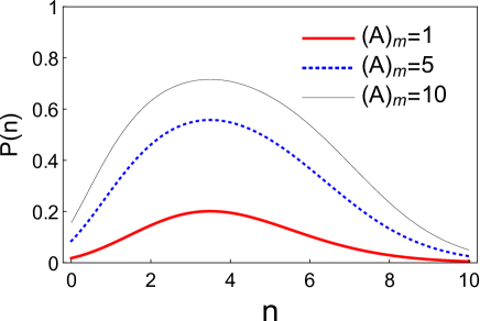
Figure 1: (Color online) For coherent state: the probability $p(n)$ versus $n$ curves with various modular values. Here, $\gamma=2$, $\phi=0$ $g=\frac{\pi}{2},\text{$\varphi_{1}=\frac{\pi}{2}$}$ and $N=1$.

Next, we determine the $Q_{M}$ parameter for a coherent state. Using the normalized final state of the coherent pointer state

$$|\varphi^{\prime}\rangle=\frac{1}{\delta^{\prime}}\sum_{n}c_{n}^{\prime}(A)_{G}|n\rangle,$$ (17)

with $\delta^{\prime}=[1-|c_{m}^{\prime}|^{2}+|c_{m}^{\prime}|^{2}||(A)_{mod}|^{2}]^{\frac{1}{2}}$, we can obtain

$$\langle a^{\dagger}a\rangle=\frac{e^{-|\alpha|^{2}}}{|\delta^{\prime}|^{2}}\{|\alpha|^{2}e^{|\alpha|^{2}}-\frac{|\alpha|^{2m}m}{m!}[1-|(A)_{m}|^{2}]\}$$ (18)

and

$$\langle a^{\dagger 2}a^{2}\rangle=\frac{e^{-|\alpha|^{2}}}{|\delta^{\prime}|^{2}}\{|\alpha|^{4}e^{|\alpha|^{2}}-\frac{|\alpha|^{2m}m(m-1)}{m!}(1-|(A)_{m}|^{2})\}$$ (19)

respectively.

We know that without interaction, $Q_{M}=0$ for a coherent state, but the negativity of $Q_{M}$ can definitely measure the non-classicality of the field. From fig. 2, when the modular value is not equal to one (there is no interaction between the system and pointer), the factor $Q_{M}$ will always be negative in some region. Furthermore, if we increase the modular value, its negativity tends to $Q_{M}=-1$, which corresponds to the Fock state with increasing coherent state parameter $\alpha$. The coherent state is a typical semi-classical field, but as seen in Fig. $(\ref{fig:fig.2})$, the generalized post-selected measurement can change its field characteristics more dramatically with increasing modular value.

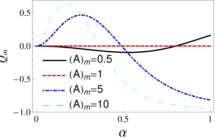
Figure 2: (Color online) The Mandel $Q_{m}$ parameter as a function of $\alpha$ for a coherent state. Here, $\gamma=\alpha,\phi=0,$ $m=2$, and other parameters are the same as in Fig. 1.

To investigate the advantages of modular value in precision measurement, we check the SNR of quadrature operator $X_{\theta}$ with the considered the post-selection probability. To do this, we first calculate the expectation value of $X_{\theta}$ and $X_{\theta}^{2}$ under the normalized final state, Eq. (17), and the results are given as

$$\langle X_{\theta}\rangle=\frac{\sqrt{2}e^{-|\alpha|^{2}}}{|\delta^{\prime}|^{2}}\Re[\alpha^{\ast}\{((A)_{m}-1)\frac{|\alpha|^{2m}}{m!}+((A)_{m}^{\ast}-1)\frac{|\alpha|^{2(m-1)}}{(m-1)!}\}e^{i\theta}+e^{|\alpha|^{2}}]$$ (20)

and

$$\langle X_{\theta}^{2}\rangle =\frac{1}{|\delta^{\prime}|^{2}}\{|\alpha|^{2}+|c_{m}|^{2}(|(A)_{m}|^{2}-1)m\}+\frac{1}{2}$$

$$+\frac{1}{|\delta^{\prime}|^{2}}\Re\{\alpha^{\ast 2}e^{-|\alpha|^{2}}e^{2i\theta}[e^{|\alpha|^{2}}+((A)_{m}-1)\frac{|\alpha|^{2m}}{m!}+((A)_{m}^{\ast}-1)\frac{|\alpha|^{2(m-2)}}{(m-2)!}]\}$$ (21)

respectively. We also plot the analytical result as a function of modular value and coherent state parameter $\gamma=\alpha$, and the result is shown in Fig. 3. As indicated in Fig. 3, the SNR of $X_{\theta=0}$ increases when the coherent state parameter $\alpha>1$ has a small modular value. However, the SNR does not increase significantly with an increase in the modular value.

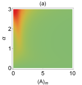
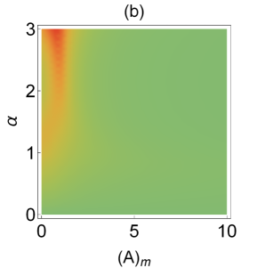
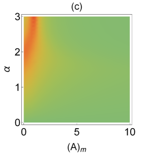
Figure 3: (Color online) SNR of quadrature operator $X$ for Coherent pointer states as a function of the modular value $(A)_{m}$ and coherent state parameter $\alpha$. Here, (a) $m=2$, (b) $m=5$, and (c) $m=10$, respectively. $\theta=0$(corresponding to the $x$ direction) and the other parameters are the same as that in Fig. 1.

III.2 Coherent Squeezed State

The coherent squeezed state is a typical quantum state. It has many applications in optical communication, optical measurement, and gravitational wave detection Milburn . Here, we assume that the initial state of the pointer is a coherent squeezed state Scully ; in the Fock-state basis, its definition can be written as

$$|\alpha,\xi\rangle =\sum_{n=0}^{\infty}\beta_{n}|n\rangle,$$ (22)

where $\gamma=\alpha\cosh r+\alpha^{\ast}e^{i\theta}\sinh r$, and

$$\beta_{n} =\frac{1}{\sqrt{\cosh r}}\exp[-\frac{1}{2}|\alpha|^{2}-\frac{1}{2}\alpha^{\ast 2}e^{i\theta}\tanh r]\times$$

$$\frac{[\frac{1}{2}e^{i\theta}\tanh r]^{\frac{n}{2}}}{\sqrt{n!}}H_{n}[\gamma(e^{i\theta}\sinh(2r))^{-\frac{1}{2}}$$ (23)

The normalized function of the coherent squeezed state after post-selection is given as

$$\left|\psi\right\rangle =\frac{1}{\eta}\{\beta_{m}[(A)_{m}-1]|m\rangle+|\alpha,\xi\rangle\}$$ (24)

where

$$\eta=[1-|\beta_{m}|^{2}+|\beta_{m}|^{2}||(A)_{mod}|^{2}]^{\frac{1}{2}}$$ (25)

As a coherent state case, we first investigate the effect of modular values on the probability of finding $n$ bosons after post-selection generalized projection measurement; the analytical result can be calculated using Eq. 13 by changing $c_{n}$ to $\beta_{n}$. As shown in Fig. 4, compared with the no interaction case, $(A)_{m}=1$, the probability of finding $n$ photons increases with increasing modular value, and this process can also be seen as a result of the amplification effect of the modular value.

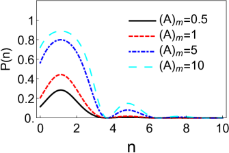
Figure 4: (Color online) The photon probability of squeezed state vs. modular value. Here, $\theta=0$, $r=0.5$, $\alpha=1$, and other parameters are the same as in Fig. 1.

As a coherent state case, to study the effect of the modular value on the field properties, we calculate the $Q_{M}$ parameter (see Eq.14) for the coherent squeezed state and discuss the analytical results. Using the normalized final state of the coherent squeezed pointer, Eq. (24), we obtain

$$\langle a^{\dagger}a\rangle=|\alpha|^{2}+\sinh^{2}r-|\beta_{m}|^{2}m(1-|(A)_{m}|^{2})$$ (26)

and

$$\langle a^{\dagger 2}a^{2}\rangle =|\alpha\cosh r-\alpha^{\ast}e^{i\theta}\sinh r|^{2}+2\sinh^{2}r\cosh^{2}r$$

$$+(|\alpha|^{2}+\sinh^{2}r)(1+|\alpha|^{2}+\sinh^{2}r)$$

$$-|\beta_{m}|^{2}(1-|(A)_{m}|^{2})m(m-1),$$ (27)

respectively.

As shown in Fig. 5, compared with the no interaction case, $(A)_{m}=1$, the $Q_{M}$ factor for the coherent squeezed state changes more and its negativity also increases with increasing modular value. Furthermore, comparing Fig. 5(a) and (b), it is clear that for the same $\alpha$ and modular value $(A)_{m}$, the negativity of the coherent squeezed state is more significant for small squeezing parameter $r$.

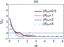
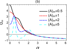
Figure 5: (Color online) The Mandel $Q_{m}$ factor squeezed coherent state as a function of coherent parameter $\alpha$ for various modular values $(A)_{m}$. Here, $m=2$ and (a) $r=0.5$, (b) $r=1$. Other parameters are the same as in Fig. 1.

For the coherent squeezed state, we also calculate the SNR of quadrature $X_{\theta}$. The expectation values of $X_{\theta}$ and $X_{\theta}^{2}$ under the normalized final coherent squeezed pointer state, Eq. (24) can be calculated as

$$\langle X_{\theta}\rangle =\frac{\sqrt{2}}{|\eta|^{2}}\times$$

$$\Re\{[\alpha^{\ast}\!\!+\!\!((A)_{m}-1)c_{m+1}^{\ast}c_{m}\sqrt{m+1}+\!\!((A)_{m}^{\ast}-1)c_{m}^{\ast}c_{m-1}\sqrt{m}]e^{i\theta}\},$$ (28)

and

$$\langle X_{\theta}\rangle^{2} =\frac{1}{|\eta|^{2}}\{|\alpha|^{2}+\sinh^{2}r+|c_{m}|^{2}(|(A)_{m}|^{2}-1)m\}+\frac{1}{2}$$

$$+\frac{1}{|\eta|^{2}}\Re[((A)_{m}^{\ast}-1)\beta_{m}^{\ast}\beta_{m-2}\sqrt{m(m-1)}e^{2i\theta}]$$

$$+\frac{1}{|\eta|^{2}}\Re\{[\alpha^{\ast 2}-e^{-i\phi}\sinh r\cosh r$$

$$+((A)_{m}-1)\beta_{m+2}^{\ast}\beta_{m}\sqrt{(m+1)(m+2)}]e^{2i\theta}\}$$ (29)

respectively.

The SNR as a function of modular value and the analytical result is shown in Fig. 6. The $SNR$ increases dramatically with increasing modular value for definite boson numbers $m$.

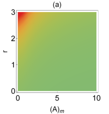
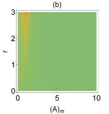
Figure 6: (Color online) The SNR of $X_{\theta=0}$ for the coherent squeezed state as a function of modular value and squeezing parameter $r$: (a) m = 2 and (b) m =5. Here, we take $\alpha=0.5$, and other parameters are the same as in Fig. 1.

III.3 Schrödinger cat state

The Schrödinger cat state, another typical quantum state, is a superposition of two coherent correlated states moving in opposite directions. Generally, there are two kinds of Schrödinger cat statesDodonov ; even and odd Schrödinger cat states. Therefore, we consider the general Schrödinger cat state as an initial pointer state in the Fock-state basis to examine the advantages of the non-classical pointer state in the generalized modular value scheme. The normalized even Schrödinger cat stateAwarwal can be written as

$$|\varphi\rangle =\mathcal{N}^{-\frac{1}{2}}(|\alpha\rangle+e^{i\varphi}|-\alpha\rangle)$$ (30)

$$=\mathcal{N}^{-\frac{1}{2}}\sum_{n=0}^{\infty}c_{n}^{\prime}|n\rangle$$ (31)

where $\mathcal{N=\mathrm{2+2e^{-2|\alpha|^{2}}\cos\varphi}},$ and $c_{n}^{\prime\prime}=e^{-\frac{|\alpha|^{2}}{2}}\frac{\alpha^{n}}{n!}(1+e^{i\varphi}(-1)^{n})$. The normalized state after the post-selected measurement is

$$|\varphi\rangle=w^{-1}\sum_{n}c_{n}^{\prime\prime}(A)_{G}|n\rangle,$$ (32)

with

$$w=[2+2e^{-2|\alpha|^{2}}\cos\varphi+|c_{n}^{\prime\prime}|^{2}(|(A)_{m}|^{2}-1)]^{\frac{1}{2}}.$$ (33)

The conditional probability of finding $n$ boson numbers of the Schrödinger cat state after generalized modular value measurement can be calculated using Eq. $(\ref{eq:cond prob})$ by changing $c_{n}$ to $c_{n}^{\prime\prime}$, and the analytical results are given in Fig. 7. Compared with the no interaction case ($(A)_{m}=1$), the conditional probability increases dramatically with increasing modular value. Furthermore, by comparing Fig. 7 $(a)$ and $(b)$, it is clear that for definite modular values, if we increase the coherent state parameter $\alpha$, the conditional probability also increases dramatically for all photon numbers and its shape resembles a periodic function.

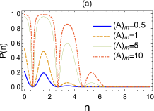
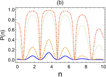
Figure 7: (Color online) The conditional probability of the Schrödinger cat state as a function of photon number $n$ with various modular values $(A)_{m}$. Here, $\varphi=\frac{\pi}{3},$ and (a)$\alpha=1$, (b) $\alpha=2$. Other parameters are the same as in Fig. 1.

Similar to the coherent state and coherent squeezed state, we investigate the effect of modular values on the field property of the Schrödinger cat state by calculating the $Q_{m}$ factor, and the analytical result is shown in Fig. 8 as a function of angle $\varphi$ for various definite modular values. From Fig. 8, we can see that compared with the no interaction case (blue dotted curve), the negativity curves become more narrow with increasing modular value, and this also can be seen as a result of the amplification effect of the modular value. Thus, we can conclude that the modular value can increase the non-classicality of states.

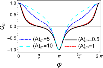
Figure 8: (Color online) The Mandel $Q_{m}$parameter as a function of $\varphi$ for the Schrodinger cat state. Here, $m=2$, $\alpha=0.2$, and other parameters are the same as in Fig. 1.

Finally, we study the SNR of quadrature operator $X_{\theta}$ of the Schrödinger cat state using the definition of SNR, i.e., Eq. $(\ref{eq:SNR})$. For the Schrödinger cat state, the expectation value of $X_{\theta}$ and its square can be given as

$$\langle\hat{X}_{\theta}\rangle =\langle\psi|\hat{X}_{\theta}|\psi\rangle$$

$$=\frac{2}{\sqrt{2}\delta^{2}}\Re[\{((A)_{m}-1)c_{m+1}^{\ast}c_{m}\sqrt{m+1}+((A)_{m}^{\ast}-1)c_{m}^{\ast}c_{m-1}\sqrt{m}$$

$$+\alpha^{\ast}(2+2i\sin\varphi e^{-2|\alpha|^{2}})\}e^{i\theta}],$$ (34)

and

$$\langle\hat{X}^{2}\rangle =\langle\psi|\hat{X}^{2}|\psi\rangle$$

$$=+\frac{1}{\delta^{2}}\Re\{[2\alpha^{2}(1+\cos\varphi e^{-2|\alpha|^{2}})+((A)_{m}-1)c_{m+2}^{\ast}c_{m}\sqrt{(m+1)(m+2)}$$

$$+((A)_{m}^{\ast}-1)c_{m}^{\ast}c_{m-2}\sqrt{m(m-1)}]e^{2i\theta}\},$$ (35)

respectively.

To study the advantages of the modular value for precision measurement with the Schrödinger cat pointer state, we plotted the SNR of the quadrature operator $X_{\theta}$ as a function of modular value $(A)_{m}$ and state parameter $\alpha$; the results are given in Fig.9. The results apparently show that the SNR increases for all The modular values with a large parameter $\alpha$; this result is different from those for the coherent and coherent squeezed pointer cases (see Fig. 3 and Fig. 6).

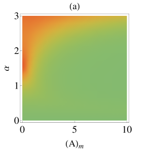
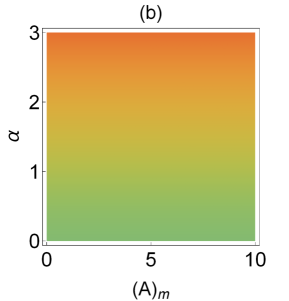
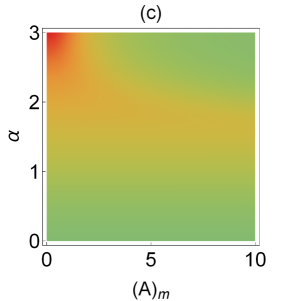
Figure 9: (Color online) SNR in the x-direction for Schrodinger pointer states with the modular value with respect to the parameter $\alpha$ (a) m = 2, (b) m = 5, and (c) m = 10. We use $\phi=0$ in equation (22) in all figures and $\theta=0$,$\varphi=0$, and other parameters are the same as in Fig. 1

IV Conclusion

We have studied the generalized modular value scheme with semi-classical and non-classical pointer states. We reported the relationship between the standard weak value and modular value. By calculating the conditional probability, $Q_{M}$ factor, and SNR of quadrature operator $X_{\theta}$ for some typical pointer states, such as the coherent state, coherent squeezed state, and Schrödinger cat state, we show the advantages of a non-classical pointer in the generalized modular value scheme compared with the semi-classical one (coherent state). We found that the conditional probabilities of finding $n$ boson numbers after post-selected measurement increased with increasing modular values. We also found that the modular values can change the negativity of the quantum field, and the non-classical field becomes more non-classical. In particular, after post-selected measurement with the modular value, the semi-classical coherent field changed to a non-classical field in some regions, and its non-classicality increased with increasing modular value. With respect to the SNR, we found that the SNR of quadrature operator $X_{\theta}$ of the coherent squeezed state and Schrödinger cat pointer state increased dramatically with increasing modular value compared with the coherent state pointer case. Our paper is a generalization of the original one-qubit pointer state modular value scheme and can be used in future works related to the application of the modular value theory with high-dimensional non-classical pointer schemes.

- (1) Y. Aharonov, D.Z. Albert, and L. Vaidman, Phys. Rev. Lett. 60, 1351 (1988).
- (2) Y. Aharonov, D. Rohrlich, Quantum Paradoxes- Quantum Theory for the Perplexed (WILEY-VCH Verlag GmbH & Co. KGaA).
- (3) A. Hosoya and Y. Shikano, J. Phys. A 43, 385307 (2010).
- (4) A. G. Kofman, S. Ashhab, and F. Nori, Phys. Rep. 520, 43 (2012).
- (5) J. Dressel, M. Malik, F. M. Miatto, A. N. Jordan, and R. W. Boyd, Rev. Mod. Phys. 86, 307 (2014).
- (6) G. C. Knee and E. M. Gauger, Phys. Rev. X 4, 011032 (2014).
- (7) X. Zhu, Y. Zhang, S. Pang, C. Qiao, Q. Liu, and S. Wu, Phys. Rev. A 84, 052111 (2011).
- (8) S. Pang and T. A. Brun, arXiv:1409.2567 (2014).
- (9) K. Nakamura, A. Nishizawa, and M. K. Fujimoto, Phys. Rev. A 85, 012113 (2012).
- (10) Y. Turek, H. Kobayashi, T. Akutsu, C. P. Sun, & Y. Shikano, New. J. Phys. 17, 083029 (2015).
- (11) Y. Turek, W. Maimaiti, Y. Shikano, C. P. Sun and M. Al-Amri, Phys.Rev. A 92, 022109 (2015).
- (12) Y. Kedem, and L. Vaidman, Phys. Rev. Lett. 105, 230401 (2010).
- (13) L. B. Ho, and N. Imoto, Phys. Lett. A 380, 2129 (2016).
- (14) L. B. Ho, and N. Imoto, Phys. Rev. A 95, 032135 (2017).
- (15) D.F. Walls and G. J. Milburn, Quantum Optics (Springer, Berlin, 1994).
- (16) M. O. Scully and M. S. Zubairy, 1997, Quantum Optics (Cambridge University Press, Cambridge, England).
- (17) G. S. Agarwal, 2013, Quantum Optics (Cambridge University Press, Cambridge, England).
- (18) V. V. Dodonov, I. A. Malkin, and V. I~ Man’ko, Physica 72, 597 (1974); I. A. Malkin and V. I. Man’ko, Dynamical Symmetries and Coherent States of Quantum Systems (Nauka, Moscow, 1979).