An efficient algorithm to test forcibly-biconnectedness of graphical degree sequences

Abstract

We present an algorithm to test whether a given graphical degree sequence is forcibly biconnected or not and prove its correctness. The worst case run time complexity of the algorithm is shown to be exponential but still much better than the previous basic algorithm presented in [14]. We show through experimental evaluations that the algorithm is efficient on average. We also adapt Ruskey et al’s classic algorithm to enumerate zero-free graphical degree sequences of length $n$ and Barnes and Savage’s classic algorithm to enumerate graphical partitions of an even integer $n$ by incorporating our testing algorithm into theirs and then obtain some enumerative results about forcibly biconnected graphical degree sequences of given length $n$ and forcibly biconnected graphical partitions of given even integer $n$. Based on these enumerative results we make some conjectures such as: when $n$ is large, (1) the proportion of forcibly biconnected graphical degree sequences of length $n$ among all zero-free graphical degree sequences of length $n$ is asymptotically a constant between 0 and 1; (2) the proportion of forcibly biconnected graphical partitions of even $n$ among all forcibly connected graphical partitions of $n$ is asymptotically 0.

Keywords— graphical degree sequence, graphical partition, forcibly biconnected, co-NP

1 Introduction

We consider graphical degree sequences of finite simple graphs (i.e. finite undirected graphs without loops or multiple edges) where the order of the terms in the sequence does not matter. As such, the terms in a graphical degree sequence is often written in non-increasing order for convenience. An arbitrary non-increasing sequence of non-negative integers $a_{1}\geq a_{2}\geq\cdots\geq a_{n}$ can be easily tested whether it is a graphical degree sequence by using the Erdős-Gallai criterion [5] or the Havel-Hakimi algorithm [7, 6]. Sierksma and Hoogeveen [12] later summarized seven equivalent criteria to characterize graphical degree sequences. A zero-free graphical degree sequence is also called a graphical partition. The former terminology is often used when the length of the sequences under consideration is fixed while the later is often used when the sum of the terms in the partitions under consideration is fixed.

Enumerating all the graphs having the same vertex degree sequence and exploring their properties have been of interest. To our knowledge, an efficient algorithm of Meringer [9] is available for the case of regular graphs, but no efficient algorithm is known to solve the problem for general graphical degree sequences. When considering all realizations of the same vertex degree sequence, two notions are very useful. Let P be any property of graphs (e.g. biconnected, critical, Hamiltonian, etc). A graphical degree sequence $\mathbf{d}=(d_{1}\geq d_{2}\geq\cdots\geq d_{n})$ is called potentially P-graphic if it has at least one realization having the property P and forcibly P-graphic if all its realizations have the property P [10]. In a previous paper [14] we have presented an efficient algorithm to test whether a graphical degree sequence is forcibly connected or not and also outline an algorithmic framework to test whether a graphical degree sequence is forcibly $k$-connected or not for every fixed $k\geq 2$. In this paper we will present a more sophisticated and efficient algorithm to test forcibly biconnectedness of graphical degree sequences. Recall that Wang and Cleitman [13] have given a simple characterization of potentially $k$-connected graphical degree sequences of length $n$, which can be performed in $O(n)$ time given any input. However, testing forcibly $k$-connectedness appears to be much harder. Some sufficient (but unnecessary) conditions are known for a graphical degree sequence to be forcibly connected or forcibly $k$-connected [3, 2, 4].

In the rest of this paper we review the basic algorithm and present the improved algorithm to characterize forcibly biconnected graphical degree sequences and give a proof why it works in Section 2. We analyze the complexity of the algorithm in Section 3. In Section 4 we demonstrate the efficiency of the algorithm through some computational experiments and then present some enumerative results regarding forcibly biconnected graphical degree sequences of given length $n$ and forcibly biconnected graphical partitions of given even integer $n$. Based on the observations on these enumerative results we make some conjectures about the relative asymptotic behavior of considered functions and the unimodality of certain associated integer sequences in Section 4.3. Finally we conclude in Section 5.

2 The testing algorithm

In this section we first review the basic algorithm to test forcibly biconnectedness proposed in [14] and then present an improved version of the algorithm. We will give a detailed proof why it correctly identifies forcibly biconnected graphical degree sequences and also comment on certain implementation issues.

2.1 Review of the basic algorithm

The basic algorithm from [14] to test forcibly biconnectedness of graphical degree sequences is shown in Algorithm 1. The idea is simple as follows. First we need to make sure that the input graphical degree sequence $\mathbf{d}$ is potentially biconnected and forcibly connected before we continue the test of forcibly biconnectedness. This is why we have lines 1 and 2.

After we confirmed this is the case, we can conclude that the input $\mathbf{d}$ is forcibly biconnected as long as we become sure that in every realization of $\mathbf{d}$ there is no cut vertex based on the definition of biconnected (non-separable) graphs. In order to simplify our discussion, we call the degree of a cut vertex in a connected graph a cut degree. Recall that we have defined in [14] that a generalized Havel-Hakimi (GHH) operation on a graphical degree sequence $\mathbf{d}$ means selecting an arbitrary term $d_{i}$ to remove from $\mathbf{d}$ and then selecting an arbitrary collection $\mathbf{d_{S}}$ of size $d_{i}$ from the remaining sequence $\mathbf{d}-\{d_{i}\}$ and decrementing each of them by 1. The resulting sequence is notationally written as $\mathbf{d^{\prime}}=GHH(\mathbf{d},d_{i},\mathbf{d_{S}})$. If $\mathbf{d^{\prime}}$ is a non forcibly connected graphical degree sequence under some choice of $d_{i}$ and $\mathbf{d_{S}}$, then the $d_{i}$ is a cut degree and $\mathbf{d}$ is not forcibly biconnected. This is because if $\mathbf{d^{\prime}}$ is non forcibly connected, i.e. it has a disconnected realization, then $\mathbf{d}$ has a connected realization with a cut vertex of degree $d_{i}$, which shows $\mathbf{d}$ is not forcibly biconnected. If no such choice of $d_{i}$ and $\mathbf{d_{S}}$ exists, then no cut degree exists and $\mathbf{d}$ is forcibly biconnected. As indicated in [14] if $\mathbf{d^{\prime}}$ obtained on line 4 is not a graphical degree sequence, then the for loop continues to iterate without returning False on line 6.

Input: A zero-free graphical degree sequence $\mathbf{d}=(d_{1}\geq d_{2}\geq\cdots\geq d_{n})$

Output: True or False, indicating whether $\mathbf{d}$ is forcibly biconnected or not

1 if $\mathbf{d}$ is not potentially biconnected or forcibly connected then

2       return False

3 for each $d_{i}$ and each collection $\mathbf{d_{S}}$ of size $d_{i}$ from $\mathbf{d}-\{d_{i}\}$ do

4       $\mathbf{d^{\prime}}\leftarrow GHH(\mathbf{d},d_{i},\mathbf{d_{S}})$;

5       if $\mathbf{d^{\prime}}$ is a non forcibly connected graphical degree sequence then

6             return False

7      

return True

Algorithm 1 basic version pseudo-code to test whether a graphical degree sequence is forcibly biconnected (See text for the description of GHH operation)

We remark that although Algorithm 1 works, its performance is probably poor due to the large number of possible choices of $d_{i}$ and $\mathbf{d_{S}}$ in the for loop from lines 3 to 6. See Section 3 for more detailed worst case run time complexity analysis. Our rudimentary implementation of Algorithm 1 can start to encounter bottlenecks for input sequences $\mathbf{d}$ of length 30 to 40.

2.2 Pseudo-code of the improved version and the proof of its correctness

Our strategy to improve Algorithm 1 is to replace the for loop from lines 3 to 6 with more sophisticated methods to find a potential cut degree. The idea is still simple. Assume there is a cut degree in the input sequence $\mathbf{d}$. Then we can construct two graphical degree sequences from $\mathbf{d}$ with total length $n+1$ of which $n-1$ come directly from $\mathbf{d}$ and the remaining two constitute a partition of the cut degree. We actually first test some necessary conditions for the existence of a cut degree, during which process an auxiliary set $\mathbf{S}$ of the orders of potential smaller induced subgraphs (explained below) is constructed should a cut degree exist. The pseudo code of the improved version is shown in Algorithm 2.

Input: A zero-free graphical degree sequence $\mathbf{d}=(d_{1}\geq d_{2}\geq\cdots\geq d_{n})$

Output: True or False, indicating whether $\mathbf{d}$ is forcibly biconnected or not

1 if $\mathbf{d}$ is not potentially biconnected or forcibly connected then

2       return False

3 if $d_{2}+d_{n}\geq n$ then

4       return True

5 $\mathbf{S}\leftarrow\varnothing$;

6 for $s\leftarrow d_{n}$ to $\lfloor(n-1)/2\rfloor$ do

7       if $d_{n-s+1}\leq s$ and $d_{2}\leq n-s-1$ then

8             $\mathbf{S}\leftarrow\mathbf{S}\cup\{s\}$

9      

10if $\mathbf{S}=\varnothing$ then

11       return True

12 foreach distinct $d$ in $\mathbf{d}$ do

13       foreach $s$ in $\mathbf{S}$ do

14             if $d=d_{1}$ or $n-s-1\geq d_{1}$ then

                   $m\leftarrow\min\{i:d_{i}\leq s\}$; // $1\leq m\leq n-s+1$

15                    $\mathbf{d_{L}}\leftarrow(d_{m}\geq d_{m+1}\geq\cdots\geq d_{n})$;

16                   Remove a copy of $d$ from $\mathbf{d_{L}}$ if it appears at least once in $\mathbf{d_{L}}$;

17                   if $\mathbf{d_{L}}$ has at least $s$ elements then

18                         Form all possible $s$ combinations $\mathbf{s_{L}}$ of $\mathbf{d_{L}}$, add an element $d^{\prime}$ with $1\leq d^{\prime}<d$ into $\mathbf{s_{L}}$ to form a sequence $\mathbf{s^{\prime}_{L}}$ of length $s+1$; Form all possible sequences $\mathbf{s_{H}}$ of length $n-s-1$ consisting of the elements of $\mathbf{d}-(\{d\}\cup\mathbf{s_{L}})$, add an element $d^{\prime\prime}=d-d^{\prime}$ ($1\leq d^{\prime\prime}<d$) into $\mathbf{s_{H}}$ to form a sequence $\mathbf{s^{\prime}_{H}}$ of length $n-s$; If both $\mathbf{s^{\prime}_{H}}$ and $\mathbf{s^{\prime}_{L}}$ have even sum and are graphical, return False;

19                        

20                  

21            

22      

23return True;

Algorithm 2 improved version pseudo-code to test whether a graphical degree sequence is forcibly biconnected

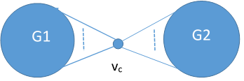
Figure 1: A realization $G$ of $\mathbf{d}$ with a cut vertex $v_{c}$.

Now we show why Algorithm 2 correctly identifies whether the input $\mathbf{d}$ is forcibly biconnected or not. The conditional test on line 1 is the same as in Algorithm 1 since potentially biconnectedness and forcibly connectedness are necessary conditions for forcibly biconnectedness. The following discussion about the pseudo code of Algorithm 2 from line 3 on all safely assumes that the input $\mathbf{d}$ is potentially biconnected and forcibly connected.

The conditional test on line 3 works because $d_{2}+d_{n}<n$ is a necessary condition for the existence of a cut degree.

Proof: Assume there is a cut vertex $v_{c}$ in a realization $G$ of $\mathbf{d}$. There are two possible situations with respect to the degree deg($v_{c}$) of $v_{c}$.

• If deg($v_{c}$) = $d_{1}$, then consider two vertices $v_{2}$ and $v_{x}$ in the two disjoint induced subgraphs $G_{1}$ and $G_{2}$ of $G$ separated by $v_{c}$ respectively such that deg($v_{2}$) = $d_{2}$ and deg($v_{x}$) is arbitrary. ($G-\{v_{c}\}$ is the disjoint union of $G_{1}$ and $G_{2}$. See Figure 1. Here the vertex degrees are all with respect to $G$.) Note that there are two possibilities regarding which induced subgraph $v_{2}$ and $v_{x}$ belong: (1) $v_{2}\in V(G_{1})$, $v_{x}\in V(G_{2})$; (2) $v_{2}\in V(G_{2})$, $v_{x}\in V(G_{1})$. It is irrelevant to us here which of the two occurs. Since $v_{2}$ and $v_{x}$ share at most one neighbor in $G$ (which is $v_{c}$) we have deg($v_{2}$)+deg($v_{x}$)$-1\leq n-2$. Thus $d_{2}+$deg($v_{x}$)$\leq n-1$. Because $d_{n}\leq$ deg($v_{x}$), we have $d_{2}+d_{n}\leq n-1$.

• If deg($v_{c}$) $<d_{1}$, then consider two vertices $v_{1}$ and $v_{x}$ in the two induced subgraphs $G_{1}$ and $G_{2}$ of $G$ separated by $v_{c}$ respectively such that deg($v_{1}$) = $d_{1}$ and deg($v_{x}$) is arbitrary. By the same argument as above we have deg($v_{1}$)+deg($v_{x}$)$-1\leq n-2$. Thus $d_{1}+$ deg($v_{x}$)$\leq n-1$. Then we have $d_{2}+d_{n}\leq n-1$ since $d_{2}\leq d_{1}$ and $d_{n}\leq$ deg($v_{x}$).

Lines 5 to 8 work as follows. If there is a cut vertex $v_{c}$ in a realization $G$ of $\mathbf{d}$ whose removal results in two disjoint induced subgraphs $G_{1}$ and $G_{2}$, then there are some restrictions on the order of the smaller of these two subgraphs given $\mathbf{d}$. Without loss of generality we assume from now on $|V(G_{2})|\leq|V(G_{1})|$ so that $G_{2}$ is always the smaller of the two disjoint subgraphs. This piece of code is trying to find out the set $\mathbf{S}$ of potential values of $|V(G_{2})|$. Notice that $G_{2}$ must contain at least $d_{n}$ vertices because if it contains at most $d_{n}-1$ vertices, then each of its vertices will have a degree at most $d_{n}-1$ in $G$, which contradicts the fact that $d_{n}$ is the smallest degree. Obviously $G_{2}$ cannot contain more than $\lfloor(n-1)/2\rfloor$ vertices since $G_{2}$ is the smaller of the two induced subgraphs separated by $v_{c}$. This explains the for loop lower bound ($d_{n}$) and upper bound ($\lfloor(n-1)/2\rfloor$) on line 6. For an integer $s$ between $d_{n}$ and $\lfloor(n-1)/2\rfloor$ to be a potential order of $G_{2}$ (i.e. $|V(G_{2})|=s$) we must have $d_{n-s+1}\leq s$ since all the vertices in $G_{2}$ have degrees at most $s$ in $G$, which makes it necessary for $\mathbf{d}$ to have at least $s$ terms that are at most $s$. The $s$ smallest terms of $\mathbf{d}$ are $d_{n-s+1}\geq d_{n-s+2}\geq\cdots\geq d_{n}$. Thus we must have $d_{n-s+1}\leq s$. If $|V(G_{2})|=s$ then $|V(G_{1})|=n-s-1$. Therefore all the vertices in $G_{1}$ have degrees at most $n-s-1$ in $G$. Now other than the requirement that $\mathbf{d}$ has at least $s$ terms that are $\leq s$, the other necessary condition for $\mathbf{d}$ to contain a cut degree is the existence of an additional $n-s-1$ terms that are at most $n-s-1$. Since $s\leq n-s-1$ based on the chosen lower and upper bounds for $s$, we must have $d_{2}\leq n-s-1$ as the other necessary condition.

The functionality of lines 9 to 10 is now clear. If no potential smaller induced subgraph order $|V(G_{2})|$ can be found in the range from $d_{n}$ to $\lfloor(n-1)/2\rfloor$, then definitely no cut degree in $\mathbf{d}$ can possibly exist and $\mathbf{d}$ must be forcibly biconnected.

After testing the necessary conditions the double for loop from lines 11 to 18 tries to find out if a cut degree $d$ in $\mathbf{d}$ exists such that the smaller subgraph $G_{2}$ after cut has order $s$ from $\mathbf{S}$.

The conditional test on line 13 is to ensure that the largest degree $d^{*}$ in $\mathbf{d}$ that is not the cut degree $d$ does not exceed the order $n-s-1$ of the larger subgraph $G_{1}$ after cut, should a cut degree $d$ exists. This is because any vertex in $G_{1}$ can only have the vertices in $G_{1}$ or the cut vertex with degree $d$ as its neighbors in $G$. If the vertex with the degree $d^{*}$ occurs in $G_{2}$, then $d^{*}$ actually should not exceed the order $s$ of $G_{2}$. However, since $s\leq n-s-1$ due to the upper bound $\lfloor(n-1)/2\rfloor$ of $s$ on line 6, it is automatically true that $d^{*}$ does not exceed $n-s-1$ when it does not exceed $s$. Now each $d$ in $\mathbf{d}$ is either $d=d_{1}$ or $d<d_{1}$. If $d=d_{1}$, then we need to ensure that $d_{2}$, which is the largest degree $d^{*}$ in $\mathbf{d}$ other than $d$, does not exceed $n-s-1$, i.e. $d_{2}\leq n-s-1$. This inequality has already been satisfied due to the conditional test on line 7. If $d<d_{1}$, then we need to ensure that $d_{1}$, which is the largest degree $d^{*}$ in $\mathbf{d}$ other than $d$, does not exceed $n-s-1$, i.e. $d_{1}\leq n-s-1$. This completes our justification of the conditional test on line 13.

Lines 14 to 16 construct the sub sequence $\mathbf{d_{L}}$ of $\mathbf{d}$ consisting exactly of those elements at most the order $s$ of the smaller subgraph $G_{2}$. The motivation for this construction is that the $s$ degrees of the vertices of $G_{2}$ must all come from $\mathbf{d_{L}}$. Note that if the cut degree $d\leq s$, then we need to remove one copy of $d$ from $\mathbf{d_{L}}$ since the cut vertex itself is not considered part of $G_{2}$. This explains why we have line 16.

The conditional test on line 17 is to ensure that there are enough degrees $\leq s$ from $\mathbf{d}$ for $G_{2}$. The sequence $\mathbf{d_{L}}$ constitutes the pool of degrees we can select for the vertex degrees of $G_{2}$. Since $G_{2}$ has order $s$ and each of its vertices has degree $\leq s$, we need $\mathbf{d_{L}}$ to have at least $s$ elements.

Line 18 performs exhaustive enumerations to find out if there are two graphical degree sequences $\mathbf{s^{\prime}_{H}}$ and $\mathbf{s^{\prime}_{L}}$, which are the vertex degree sequences of $G-V(G_{2})$ and $G-V(G_{1})$ respectively, should a cut degree $d$ exists such that the smaller subgraph $G_{2}$ is of order $s$ after cut. The vertex degree sequence $\mathbf{s^{\prime}_{L}}$ of $G-V(G_{1})$ consists of the $s$ degrees of the vertices of $G_{2}$ in $G$ together with the degree $d^{\prime}$ equal to the number of adjacencies of the cut vertex with $G_{2}$. The vertex degree sequence $\mathbf{s^{\prime}_{H}}$ of $G-V(G_{2})$ consists of the $n-s-1$ degrees of the vertices of $G_{1}$ in $G$ together with the degree $d^{\prime\prime}=d-d^{\prime}$ equal to the number of adjacencies of the cut vertex with $G_{1}$. Clearly, one level of exhaustive enumeration comes from selecting $s$ degrees $\mathbf{s_{L}}$ from $\mathbf{d_{L}}$. The other level of exhaustive enumeration comes from choosing $d^{\prime}$ ($1\leq d^{\prime}<d$), which is the number of adjacencies of the cut vertex with $G_{2}$. Notationally we have $\mathbf{s^{\prime}_{L}}=\mathbf{s_{L}}\cup\{d^{\prime}\}$. Once $\mathbf{s_{L}}$ from $\mathbf{d_{L}}$ and $d^{\prime}$ ($1\leq d^{\prime}<d$) have been chosen, $\mathbf{s^{\prime}_{L}}$ and $\mathbf{s^{\prime}_{H}}$ are both determined, with $\mathbf{s^{\prime}_{H}}=(\mathbf{d}-(\{d\}\cup\mathbf{s_{L}}))\cup\{d^{\prime\prime}\}$. We only need a linear time algorithm such as from [8] to test whether $\mathbf{s^{\prime}_{L}}$ and $\mathbf{s^{\prime}_{H}}$ are both graphical. If during the double for loop from lines 11 to 18 such a pair of graphical degree sequences $\mathbf{s^{\prime}_{L}}$ and $\mathbf{s^{\prime}_{H}}$ can be found, then we know that the input $\mathbf{d}$ is not forcibly biconnected (hence returning False on line 18) since we have found a cut degree $d$ together with the degrees for vertices of $G_{1}$ and $G_{2}$ after cut and the number of adjacencies $(d^{\prime\prime},d^{\prime})$ of the cut vertex with $G_{1}$ and $G_{2}$ respectively. If no such pair of graphical degree sequences $\mathbf{s^{\prime}_{L}}$ and $\mathbf{s^{\prime}_{H}}$ can ever be found on line 18, then we know that the input $\mathbf{d}$ is forcibly biconnected and we should return True on line 19.

One thing to note about Algorithm 2 is that the sequences mentioned from line 15 to line 18 are all treated as multisets so that the set difference and set union operations therein should be implemented as multiset operations. We also note that Algorithm 2 performs a test of whether any graphical sequence is forcibly connected or not at most once (on line 1), while Algorithm 1 possibly performs such a test many times (on lines 1 and 5). This is a supplementary explanation of why Algorithm 2 performs much better than Algorithm 1 on many inputs. More detailed run time analysis is presented later.

2.3 Extensions of the algorithm

In this section we briefly discuss how to extend Algorithm 2 to perform the additional task of listing all possible cuts of a potentially biconnected and forcibly connected but non forcibly biconnected graphical degree sequence. We also show that the idea of Algorithm 2 to find a cut degree in determining forcibly biconnectedness can be extended to test forcibly triconnectedness of a graphical degree sequence and beyond.

2.3.1 Enumeration of all possible cuttings

It is easy to see that if the input $\mathbf{d}$ is potentially biconnected and forcibly connected but not forcibly biconnected, we can enumerate all possible cuttings (the cut degree, the numbers of adjacencies of the cut vertex to $G_{1}$ and $G_{2}$ and the degrees of the vertices of $G_{1}$ and $G_{2}$ in $G$ using the notation of Section 2.2). We simply need to report such a cutting on line 18 of Algorithm 2 without returning False immediately. Such an enumerative algorithm to find all possible cuttings of the input $\mathbf{d}$ can be useful when we want to explore the possible realizations of $\mathbf{d}$ and their properties.

2.3.2 Testing forcibly $k$-connectedness of $\mathbf{d}$ when $k\geq 3$

The idea to find a cut degree in Algorithm 2 can be extended to find a pair of cut degrees for the case of $k=3$ and a triple of cut degrees for the case of $k=4$, and so on. Now we need to consider more complicated situations about whether those cut vertices with potential cut degrees are themselves adjacent or not, besides the numbers of adjacencies of each of these cut vertices to $G_{1}$ and $G_{2}$ and the potential orders of $G_{1}$ and $G_{2}$. However, we believe a careful implementation should still have better performance than the basic version to test forcibly $k$-connectedness presented in [14].

3 Complexity analysis

In this section we give a rough and conservative analysis of the worst case run time performance of Algorithms 1 and 2. We also comment on the computational complexity of the decision problem of testing forcibly biconnectedness of graphical degree sequences.

Let us first consider the basic Algorithm 1.

The test of potentially biconnectedness on line 1 can be performed in linear time using the Wang and Cleitman characterization [13]. The test of forcibly connectedness on line 1 has been analyzed in [14] with worst case run time probably exponential (around $poly(n)\binom{n}{n/2}$ where $poly(n)$ is some polynomial of $n$).

The number of iterations of the body of the for loop from lines 3 to 6 depends on the number of possible choices of $d_{i}$ and $\mathbf{d_{S}}$. The number of choices for $d_{i}$ is $O(n)$. The number of choices of $\mathbf{d_{S}}$ after $d_{i}$ is chosen depends on the magnitude of $d_{i}$. Assume the average size of $d_{i}$ is $n/2$ for the purpose of simplicity of our analysis. The number of choices of $\mathbf{d_{S}}$ is then about $\binom{n-1}{n/2}$ since $\mathbf{d_{S}}$ is to be chosen from $\mathbf{d}-\{d_{i}\}$. Once $d_{i}$ and $\mathbf{d_{S}}$ have been chosen, the sequence $\mathbf{d^{\prime}}$ of length $n-1$ can be constructed and tested whether it is a graphical sequence in $O(n)$ time. After that the testing of forcibly connectedness of $\mathbf{d^{\prime}}$ can be done in $poly(n-1)\binom{n-1}{(n-1)/2}$ time. Thus we can see that the worst case run time complexity of the for loop from lines 3 to 6 is roughly $poly(n)\binom{n}{n/2}^{2}$ under this simplified analysis.

The total run time complexity of Algorithm 1 is dominated by the for loop from lines 3 to 6, which is about $poly(n)\binom{n}{n/2}^{2}$.

Let us now turn to the improved Algorithm 2.

The worst case run time of line 1 to test potentially biconnectedness and forcibly connectedness is about $poly(n)\binom{n}{n/2}$ as shown above.

It is easy to see that lines 3 to 10 take linear time. The body of the double for loops from line 13 to 18 will be iterated at most $O(n^{2})$ times since we have $O(n)$ distinct $d$ in $\mathbf{d}$ and less than $n/2$ elements in $\mathbf{S}$. Lines 14 to 16 clearly take $O(n)$ time. Thus, the total run time excluding the test of forcibly connectedness on line 1 and the exhaustive enumeration on line 18 is $O(n^{3})$.

Now we consider line 18. The length of the sequence $\mathbf{d_{L}}$ could be up to $n$ and the length $s$ of the sequence $\mathbf{s_{L}}$ could be up to $\lfloor(n-1)/2\rfloor$. Then the maximum number of all possible choices of $\mathbf{s_{L}}$ from $\mathbf{d_{L}}$ will be up to $\binom{n}{\lfloor(n-1)/2\rfloor}$, which is exponential. The number of choices for $d^{\prime}$ is $O(n)$. Once the choices for $\mathbf{s_{L}}$ and $d^{\prime}$ have been made, the two sequences $\mathbf{s^{\prime}_{L}}$ and $\mathbf{s^{\prime}_{H}}$ can be constructed and tested whether they are graphical in $O(n)$ time. This shows that the worst case total run time of line 18 is about $poly(n)\binom{n}{n/2}$.

The most time consuming parts of Algorithm 2 are the testing of forcibly connectedness on line 1 and the exhaustive enumeration on line 18. In the worst case both of these parts can take exponential time. The combined worst case total run time of Algorithm 2 is then about $poly(n)\binom{n}{n/2}$, which can be seen to be better than the worst case run time of Algorithm 1 by a factor of $\binom{n}{n/2}$. Suitable data structures can be established for those multiset sequences mentioned on line 18 to avoid duplicate exhaustive enumerations. However, a large number of exhaustive enumerations on line 18 before returning can happen for some inputs based on our computational experiences.

As for the computational complexity of the problem of deciding forcibly biconnectedness of arbitrary graphical degree sequences, it is known to be in co-NP as indicated in [14]. However we do not know if it is co-NP-hard or if it is inherently harder than the problem of deciding forcibly connectedness of arbitrary graphical degree sequences. In general one can be interested in whether the problem of deciding forcibly $k$-connectedness is inherently harder than the problem of deciding forcibly $(k-1)$-connectedness for any fixed $k$.

4 Computational results

In this section we will first present some results on the experimental evaluation on the performance of Algorithm 2 on randomly generated graphical degree sequences. We will then provide some enumerative results about the number of forcibly biconnected graphical degree sequences of given length and the number of forcibly biconnected graphical partitions of a given even integer. Based on these enumerative results we will make some conjectures about the relative asymptotic behavior of related functions and the unimodality of certain associated integer sequences.

Before we continue we remark that Algorithm 1 can only satisfactorily process inputs with length below 50 most of the time unless the input is not potentially biconnected or it can be easily determined to be non forcibly connected.

4.1 Performance evaluations of Algorithm 2

Previously in [14] we evaluated our algorithm to test forcibly connectedness of graphical degree sequences using randomly generated long inputs with length up to 10000. In anticipation of the greater challenge to test forcibly biconnectedness (even though the worst case time complexity of the algorithm in [14] to test forcibly connectedness and Algorithm 2 here differ by at most a polynomial factor as shown in Section 3), we decide to evaluate Algorithm 2 using randomly generated inputs with length up to 1000.

We adopt a similar evaluation methodology as in [14]. Choose a constant $p_{l}$ in the range [0.002,0.49] and a constant $p_{h}$ in the range [$p_{l}+0.01$,0.99] and generate 100 random graphical degree sequences of length $n$ with largest term around $p_{h}n$ and smallest term around $p_{l}n$. For each chosen length $n$, the smallest chosen $p_{l}$ is slightly adjusted to make sure that the smallest term in each generated random input graphical degree sequence is at least 2 since any graphical degree sequence with the smallest term 1 is not potentially biconnected so the answer is always False for such inputs. The largest $p_{l}$ is chosen to be 0.49 because any graphical degree sequence of length $n$ with smallest term at least $0.5n$ is not only forcibly connected (see [14]) but also forcibly biconnected (see line 3 of Algorithm 2). The constant $p_{h}$ is chosen to be less than 1 so that the largest term in any randomly generated input graphical degree sequence is at most $n-1$.

We implemented our Algorithm 2 using C++ and compiled it using g++ with optimization level -O3. The experimental evaluations are performed on a common Linux workstation. We run the code on the randomly generated instances and record the average performance and note the proportion of them that are forcibly biconnected. Table 1 lists the tested $p_{l}$ and $p_{h}$ for the input length $n=500$. The input lengths that are chosen to be tested are $n=20,30,\cdots,100,200,\cdots,1000$. The chosen $p_{l}$ and $p_{h}$ for different input length $n$ are all similar to the case for $n=500$.

Table 1: Chosen $p_{l}$ and $p_{h}$ in the experimental performance evaluation of Algorithm 2 for input length $n=500$.

$p_{l}$	$p_{h}$
0.01	0.02,0.03,…,0.1,0.2,0.3,…,0.7,0.8,0.9,0.95,0.97,0.99
0.03	0.04,0.05,…,0.1,0.2,0.3,…,0.72,0.73,0.74,0.75,0.8,0.85,0.9,0.94,0.96,0.99
0.06	0.08,0.1,0.2,…,0.7,0.71,0.73,0.77,0.8,0.85,0.88,0.89,0.95,0.99
0.1	0.15,0.25,0.35,…,0.65,0.68,0.7,0.75,0.8,0.82,0.85,0.9
0.2	0.3,0.4,0.5,0.6,0.62,0.65,0.68,0.7,0.8,0.9
0.3	0.35,0.45,0.55,0.56,0.58,0.6,0.62,0.7,0.8,0.9
0.4	0.44,0.48,0.52,0.53,0.54,0.55,0.56,0.6,0.7,0.8,0.9
0.49	0.491,…,0.499,0.5,0.501,0.502,0.504,0.506,0.508,0.51,0.52,…,0.6,0.7,0.8,0.9

We summarize our experimental evaluation results as follows.

1. For all input length $n$ below 100, all instances can be decided instantly (run time $<0.1s$).

2. Starting from $n=100$ up to $n=1000$, certain inputs start to cause Algorithm 2 to run slowly (run time from a few seconds to a few hours or time out). The longer the length $n$, the more time these difficult instances might take and the higher percentage of these difficult instances occupy in all 100 input instances for a given triple of ($n,p_{l},p_{h}$). In detail, difficult instances could occur when (1) $p_{l}$ is very small (say from 0.005 to 0.05) and $p_{h}$ is very large (say from 0.8 to 0.95) or when (2) $p_{l}$ is slightly below 0.5 and $p_{h}$ is slightly above 0.5. We note based on our observations that the former situation (1) often (but not always) corresponds to the cases where forcibly connectedness itself is hard to decide while the latter situation (2) corresponds to the cases where forcibly connectedness itself is not hard to decide but forcibly biconnectedness is after confirmation of forcibly connectedness.

3. For each fixed $p_{l}$, there is a transition range of $p_{h}$ (shown in bold in Table 1) such that (1) if $p_{h}$ is below this transition range, almost all input instances are non forcibly biconnected; (2) if $p_{h}$ is above this transition range, almost all input instances are forcibly biconnected; (3) when $p_{h}$ increases in the transition range, the proportion of input instances that are forcibly biconnected grows approximately from 0 to 1. For example, for input length $n=500$ and $p_{l}=0.1$, the transition range of $p_{h}$ is from 0.68 to 0.8. When $p_{h}$ is below 0.68 almost all input instances are non forcibly biconnected. When $p_{h}$ is above 0.8 almost all input instances are forcibly biconnected. As noted in [14], these results indicate relative frequencies, instead of absolute law, of forcibly biconnected graphical degree sequences among the pool of all graphical degree sequences that can be chosen to test.

To sum up, our implementation of Algorithm 2 runs fast on the majority of the tested random inputs with length up to 1000. Considering that all those inputs with smallest term exactly 1 or at least $n/2$ are excluded from test, which are estimated to occupy at least 35% of all possible instances, we are confident that Algorithm 2 is efficient on average. Certain inputs do cause it to perform poorly. In particular, if it is hard to decide whether a potentially biconnected input is forcibly connected using the algorithm in [14], it is also hard to decide whether it is forcibly biconnected using Algorithm 2 since testing forcibly connectedness is part of testing forcibly biconnectedness. We also remark from our experimental observations that there are difficult input instances whose hardness come mainly from deciding forcibly connectedness. That is, the algorithm may take a long time to decide forcibly connectedness. However, once the algorithm knows the input is potentially biconnected and forcibly connected it can almost instantly finish the testing of forcibly biconnectedness. There are also difficult input instances that are easy to be determined to be potentially biconnected and forcibly connected but hard to be further determined to be forcibly biconnected. Finally, there are some difficult input instances that are hard to be determined to be forcibly connected and, after confirmation of forcibly connectedness, hard to be further determined to be forcibly biconnected.

Table 2: Terminology used in Section 4.2

Term	Meaning
$D(n)$	number of zero-free graphical sequences of length $n$
$D_{k\_c}(n)$	number of potentially $k$-connected graphical sequences of length $n$
$D_{k\_f}(n)$	number of forcibly $k$-connected graphical sequences of length $n$
$C_{k}[n,N]$	number of potentially $k$-connected graphical degree sequences
	of length $n$ with degree sum $N$
$F_{k}[n,N]$	number of forcibly $k$-connected graphical degree sequences
	of length $n$ with degree sum $N$
$L_{k}[n,j]$	number of forcibly $k$-connected graphical degree sequences of
	length $n$ with largest term $j$
$M_{k}(n)$	minimum largest term in any forcibly $k$-connected graphical
	sequence of length $n$
$g(n)$	number of graphical partitions of even $n$
$g_{k\_c}(n)$	number of potentially $k$-connected graphical partitions of even $n$
$g_{k\_f}(n)$	number of forcibly $k$-connected graphical partitions of even $n$
$c_{k}[n,j]$	number of potentially $k$-connected graphical partitions of
	even $n$ with $j$ parts
$f_{k}[n,j]$	number of forcibly $k$-connected graphical partitions of
	even $n$ with $j$ parts
$l_{k}[n,j]$	number of forcibly $k$-connected graphical partitions of $n$ with largest term $j$
$m_{k}(n)$	minimum largest term of forcibly $k$-connected graphical partitions of $n$

4.2 Enumerative results

In this section we present some enumerative results related to forcibly biconnected graphical degree sequences of given length and forcibly biconnected graphical partitions of given even integer. We also make some conjectures based on these enumerative results. For the reader’s convenience, we list the notations and their meanings used in this section in Table 2. Note that $C_{k}[n,N]=c_{k}[N,n]$ and $F_{k}[n,N]=f_{k}[N,n]$ by definition.

In a previous manuscript [15] we presented efficient algorithms to compute $D(n)$ and $D_{k\_c}(n)$ for fixed $k$ and have shown that $\lim_{n\to\infty}\frac{D_{1\_c}(n)}{D(n)}=1$ and $\lim_{n\to\infty}\frac{D_{2\_c}(n)}{D(n)}\neq 1$. Recently in [14] we presented enumerative results about the number $D_{1\_f}(n)$ of forcibly connected graphical degree sequences of length $n$ and conjectured that $\lim_{n\to\infty}\frac{D_{1\_f}(n)}{D(n)}=1$. Using the sandwich theorem of calculus we can easily see that $\lim_{n\to\infty}\frac{D_{2\_f}(n)}{D(n)}\neq 1$ since $D_{2\_f}(n)\leq D_{2\_c}(n)\leq D(n)$. We adapted the algorithm of Ruskey et al [11] that enumerates zero-free graphical degree sequences of length $n$ by incorporating the test in Algorithm 2 to enumerate those that are forcibly biconnected. The results together with the proportion of them in all forcibly connected graphical degree sequences of length $n$ and in all zero-free graphical degree sequences of length $n$ are listed in Table 3. From Table 3 it looks likely that $D_{2\_f}(n)/D_{1\_f}(n)$ and $D_{2\_f}(n)/D(n)$ both tend to some constant less than 1. Note that if the conjecture $\lim_{n\to\infty}\frac{D_{1\_f}(n)}{D(n)}=1$ is true, then $\lim_{n\to\infty}\frac{D_{2\_f}(n)}{D_{1\_f}(n)}\neq 1$ since we know $\lim_{n\to\infty}\frac{D_{2\_f}(n)}{D(n)}\neq 1$.

Table 3: Number of forcibly biconnected graphical sequences of length $n$ and their proportions in forcibly connected and zero-free graphical sequences of length $n$ respectively.

$n$	$D_{2\_f}(n)$	$D_{1\_f}(n)$	$D_{2\_f}(n)/D_{1\_f}(n)$	$D_{2\_f}(n)/D(n)$
4	3	6	0.500000	0.428571
5	9	18	0.500000	0.450000
6	30	63	0.476190	0.422535
7	105	216	0.486111	0.437500
8	381	783	0.486590	0.437428
9	1412	2843	0.496658	0.448539
10	5296	10535	0.502705	0.454397
11	20010	39232	0.510043	0.461783
12	76045	147457	0.515710	0.467196
13	290142	556859	0.521033	0.472392
14	1110847	2113982	0.525476	0.476649
15	4264563	8054923	0.529436	0.480473
16	16411152	30799063	0.532846	0.483750
17	63284616	118098443	0.535863	0.486662
18	244489774	454006818	0.538516	0.489220
19	946101866	1749201100	0.540877	0.491504
20	3666602417	6752721263	0.542981	0.493542
21	14229131559	26114628694	0.544872	0.495376
22	55288167003	101153550972	0.546577	0.497033
23	215070591363	392377497401	0.548122	0.498537
24	837503686065	1524043284254	0.549527	0.499908
25	3264489341370	5926683351876	0.550812	0.501162

In Table 4 we show itemized potentially and forcibly biconnected graphical degree sequences of length 7 based on the degree sum $N$. The counts for $N<14$ are not shown because those counts are all 0. The minimum $N$ such that $C_{2}[7,N]$ is nonzero can be easily determined to be 14 using the Wang and Cleitman [13] characterization. However, the minimum $N$ such that $F_{2}[7,N]$ is nonzero (which is equal to 20, not 14) is not obvious. In general for given $n$ if the minimum $N$ such that $F_{2}[n,N]$ is nonzero can be easily determined, it can be added into Algorithm 2 so that for any input $\mathbf{d}$ with the sum of its terms less than this minimum the algorithm can immediately return False. The largest degree sum is 42 for any graphical degree sequence of length 7. Notice that both the nonzero $C_{2}[7,N]$ values and the nonzero $F_{2}[7,N]$ values when $N$ increases form a unimodal sequence. Also notice that $C_{2}[7,N]=F_{2}[7,N]$ when $28\leq N\leq 42$. This shows that for even $N$ between 28 and 42, all potentially biconnected graphical partitions of $N$ with 7 parts are also forcibly biconnected. That is, 28 is the smallest $N$ such that all potentially biconnected graphical partitions of $N$ with 7 parts are also forcibly biconnected.

Table 4: Number of potentially (row $C_{2}[7,N]$) and forcibly (row $F_{2}[7,N]$) biconnected graphical degree sequences of length 7 with given degree sum $N$.

degree sum $N$	14	16	18	20	22	24	26	28	30	32	34	36	38	40	42
$C_{2}[7,N]$	1	1	3	7	14	17	18	19	16	12	8	5	2	1	1
$F_{2}[7,N]$	0	0	0	2	8	14	17	19	16	12	8	5	2	1	1

In Table 5 we show itemized numbers of forcibly biconnected graphical degree sequences of length 15 based on the largest degree. The counts for largest degrees less than 7 are not shown because those counts are all 0. Any graphical degree sequence of length 15 has a largest term at most 14. From the table we can see that the counts decrease when the largest degree decreases. For other degree sequence lengths from 5 to 25 we observed similar behavior. The table also indicates that there are no forcibly biconnected graphical degree sequences of length 15 with largest degree less than 7. In fact, we can define $M_{2}(n)$ to be the minimum largest term in any forcibly biconnected graphical sequence of length $n$. This is, $M_{2}(n)\doteq$ min{$\Delta$: $\Delta$ is the largest term of some forcibly biconnected graphical degree sequence of length $n$}. Clearly we have $M_{2}(n)\leq n/2$ since for even $n$ the sequence $n/2,n/2,\cdots,n/2$ of length $n$ is forcibly biconnected. In [14] we have defined $M(n)$ to be the minimum largest term in any forcibly connected graphical sequence of length $n$ ($M(n)=M_{1}(n)$ based on the notation $M_{k}(n)$ in Table 2). By definition we obviously have $M_{2}(n)\geq M(n)$ so that we also have $M_{2}(n)>c\sqrt{n}$ for all sufficiently large $n$ and some constant $c>0$ based on a lower bound of $M(n)$ shown in [14]. If $M_{2}(n)$ can be easily calculated, it can be added into Algorithm 2 so that any input $\mathbf{d}$ of length $n$ with largest term less than $M_{2}(n)$ can be immediately decided to be non forcibly biconnected. We show the values of $M_{2}(n)$ and $M(n)$ based on our enumerative results in Table 6.

Table 5: Number $L_{2}[15,j]$ of forcibly biconnected graphical degree sequences of length 15 with given largest term $j$.

largest part $j$	14	13	12	11	10	9	8	7
$L_{2}[15,j]$	2113982	1335151	573980	185510	45951	8689	1202	98

Table 6: Minimum largest term $M_{2}(n)$(resp. $M(n)$) of forcibly biconnected (resp. connected) graphical sequences of length $n$.

$n$	4	5	6	7	8	9	10	11	12	13	14
$M_{2}(n)$	2	2	3	3	4	4	4	5	5	6	6
$M(n)$	2	2	3	3	3	4	4	5	5	5	6
$n$	15	16	17	18	19	20	21	22	23	24	25
$M_{2}(n)$	7	7	7	8	8	9	9	10	10	10	11
$M(n)$	6	6	7	7	7	7	8	8	8	8	8

We also incorporated our Algorithm 2 into the highly efficient Constant Amortized Time (CAT) algorithm of Barnes and Savage [1] to generate forcibly biconnected graphical partitions of even $n$. The results for $n$ up to 170 together with the proportion of them in all forcibly connected graphical partitions of $n$ are listed in Table 7. For the purpose of saving space we only show the results in increments of 10 for $n$. From the table it seems reasonable to conclude that the proportion $g_{2\_f}(n)/g_{1\_f}(n)$ will decrease when $n$ is beyond some small threshold and it might tend to the limit 0. Previously in [14] we have conjectured that $\lim_{n\to\infty}\frac{g_{1\_f}(n)}{g(n)}=0$. With the trend of $g_{2\_f}(n)/g_{1\_f}(n)$ in Table 7, we are almost certain that $\lim_{n\to\infty}\frac{g_{2\_f}(n)}{g(n)}=0$.

Table 7: Number of forcibly biconnected graphical partitions of $n$ and their proportions in all forcibly connected graphical partitions of $n$.

$n$	$g_{2\_f}(n)$	$g_{1\_f}(n)$	$g_{2\_f}(n)/g_{1\_f}(n)$
10	2	8	0.250000
20	10	81	0.123457
30	55	586	0.093857
40	262	3308	0.079202
50	1062	15748	0.067437
60	4171	66843	0.062400
70	14445	256347	0.056349
80	47586	909945	0.052295
90	147132	3026907	0.048608
100	430709	9512939	0.045276
110	1217258	28504221	0.042704
120	3285793	81823499	0.040157
130	8621222	226224550	0.038109
140	21874986	604601758	0.036181
150	54077294	1567370784	0.034502
160	130279782	3951974440	0.032966
170	306808321	9714690421	0.031582

When generating all forcibly biconnected graphical partitions of $n$ we can also output the itemized counts based on the number of parts or the largest part. In Table 8 we show itemized counts of potentially biconnected and forcibly biconnected graphical partitions of 30 based on the number of parts. The counts $c_{2}[30,j]$ and $f_{2}[30,j]$ for which the number of parts $j$ is less than 6 or greater than 15 are not shown because those counts are all 0. When $n$ is large, the minimum number of parts $j$ for which $c_{2}[n,j]$ and $f_{2}[n,j]$ are both nonzero is clearly the smallest positive integer $j(n)$ such that $j(n)(j(n)-1)\geq n$. The largest number of parts $j$ for which $c_{2}[n,j]$ is nonzero is clearly $n/2$ since the sequence $2,\cdots,2$ ($n/2$ copies) is potentially biconnected. The largest number of parts $j$ for which $f_{2}[n,j]$ is nonzero does not appear to be easily computable. Note that the nonzero values of $c_{2}[30,j]$ and $f_{2}[30,j]$ both form a unimodal sequence when $j$ increases. Also note that $c_{2}[30,j]=f_{2}[30,j]$ for $j=6,7$. This shows that all potentially biconnected graphical partitions of 30 with 6 or 7 parts are also forcibly biconnected. That is, 7 is the largest number of parts $j$ such that all potentially biconnected graphical partitions of 30 with $j$ parts are also forcibly biconnected. The fact that $c_{2}[30,7]=f_{2}[30,7]=16$ agrees with the result that $C_{2}[7,30]=F_{2}[7,30]=16$ in Table 4.

Table 8: Number of potentially (row $c_{2}[30,j]$) and forcibly (row $f_{2}[30,j]$) biconnected graphical partitions of 30 with given number of parts $j$.

number of parts $j$	6	7	8	9	10	11	12	13	14	15
$c_{2}[30,j]$	1	16	44	54	30	15	7	3	1	1
$f_{2}[30,j]$	1	16	30	8	0	0	0	0	0	0

Table 9: Number $l_{2}[30,j]$ of forcibly biconnected graphical partitions of 30 with given largest term $j$.

largest part $j$	4	5	6	7	8
$l_{2}[30,j]$	2	13	23	13	4

In Table 9 we show itemized counts of forcibly biconnected graphical partitions of 30 based on the largest term. The counts $l_{2}[30,j]$ for which the largest part $j$ is less than 4 or greater than 8 are not shown since those counts are all 0. The nonzero counts $l_{2}[30,j]$ form a unimodal sequence. Given $n$ the largest $j$ for which $l_{2}[n,j]$ is nonzero can be easily determined by solving the inequality $n\geq 2(j+1)-4+2j$ using the Wang and Cleitman [13] characterization since a potentially biconnected graphical degree sequence of length $j+1$ and largest term $j$ is forcibly biconnected. However, the smallest $j$ for which $l_{2}[n,j]$ is nonzero does not appear to be easily computable. If we use $m_{2}(n)$ to denote this smallest $j$, i.e. the minimum largest term of any forcibly biconnected graphical partitions of $n$, then we clearly have $2\leq m_{2}(n)\leq\sqrt{n}$. We show the values of $m_{2}(n)$ for some small $n$ based on our enumerative results in Table 10. The fact that $m_{2}(30)=4$ agrees with the fact that in Table 9 the counts $l_{2}[30,j]$ are all 0 for largest part $j$ less than 4. In [14] we have defined $m(n)$ as the minimum largest term of any forcibly connected graphical partition of $n$ ($m(n)=m_{1}(n)$ in the notation $m_{k}(n)$ of Table 2). Clearly we have $m(n)\leq m_{2}(n)$ by definition. We can see that $m_{2}(n)$ happen to agree with $m(n)$ for those $n$ listed in Table 10.

Table 10: Minimum largest term $m_{2}(n)$ (resp. $m(n)$) of forcibly biconnected (resp. connected) graphical partitions of $n$.

$n$	10	20	30	40	50	60	70	80	90	100
$m_{2}(n)$	2	3	4	5	5	6	6	6	7	7
$m(n)$	2	3	4	5	5	6	6	6	7	7

4.3 Questions and conjectures

Based on the obtained enumerative results we ask the following questions and make certain conjectures:

1. What is the growth order of $D_{2\_f}(n)$ relative to $D_{1\_f}(n)$ and $D(n)$? We conjecture that both $\frac{D_{2\_f}(n)}{D_{1\_f}(n)}$ and $\frac{D_{2\_f}(n)}{D(n)}$ tend to a constant less than 1. Is it true that $\lim_{n\to\infty}\frac{D_{2\_f}(n)}{D_{2\_f}(n-1)}=4$? Furthermore, we conjecture that $\frac{D_{2\_f}(n)}{D_{1\_f}(n)}$ and $\frac{D_{2\_f}(n)}{D(n)}$ are both monotonically increasing when $n\geq 8$. What can be said about the relative orders of $D_{k\_c}(n)$, $D_{k\_f}(n)$ and $D(n)$ when $k\geq 3$?

2. What is the growth order of $g_{2\_f}(2n)$ relative to $g_{1\_f}(2n)$ and $g(2n)$? We conjecture that $\lim_{n\to\infty}\frac{g_{2\_f}(2n)}{g_{1\_f}(2n)}=0$ and $\lim_{n\to\infty}\frac{g_{2\_f}(2n)}{g(2n)}=0$. Furthermore, we conjecture that $g_{2\_f}(2n)/g_{1\_f}(2n)$ is monotonically decreasing when $n\geq 5$. Is it true that $\lim_{n\to\infty}\frac{g_{k\_f}(2n)}{g_{k-1\_f}(2n)}=0$ for fixed $k\geq 3$?

3. We conjecture that the numbers $F_{2}(n,N)$ of forcibly biconnected graphical degree sequences of length $n$ with degree sum $N$, when $N$ runs through $2n-2,2n,\cdots,n(n-1)$, give a unimodal sequence. (There may be some zeros in the sequence.)

4. Let $t(n)$ be the smallest positive integer such that $t(n)(t(n)-1)\geq n$. We conjecture that the numbers $f_{2}(n,j)$ of forcibly biconnected graphical partitions of $n$ with $j$ parts, when $j$ runs through $t(n),t(n)+1,\cdots,n/2$, give a unimodal sequence. (There may be some zeros in the sequence.)

5. What is the growth order of $M_{2}(n)$, the minimum largest term in any forcibly biconnected graphical sequence of length $n$? Is there a constant $C>0$ such that $\lim_{n\to\infty}\frac{M_{2}(n)}{n}=C$? Is it true that $M_{2}(n)=\Theta(M(n))$? Is there an efficient algorithm to compute $M_{2}(n)$? What can be said about the growth order of $M_{k}(n)$ for fixed $k\geq 3$?

6. What is the growth order of $m_{2}(n)$, the minimum largest term in any forcibly biconnected graphical partition of $n$? Is there a constant $C>0$ such that $\lim_{n\to\infty}\frac{m_{2}(n)}{\sqrt{n}}=C$? Is there an efficient algorithm to compute $m_{2}(n)$? What can be said about the growth order of $m_{k}(n)$ for fixed $k\geq 3$?

7. We conjecture that the numbers $l_{2}(n,\Delta)$ of forcibly biconnected graphical partitions of an even $n$ with largest part exactly $\Delta$, when $\Delta$ runs through $m_{2}(n),m_{2}(n)+1,\cdots,n/2$, give a unimodal sequence. (There may be some zeros in the sequence.)

5 Conclusions

In this paper we presented an efficient algorithm to test whether a given graphical degree sequence is forcibly biconnected or not. We also discussed the possible extension of the idea used in the algorithm to test forcibly $k$-connectedness of graphical degree sequences for fixed $k\geq 3$. The worst case run time complexity of the algorithm is exponential. However, extensive performance evaluations on a wide range of random graphical degree sequences demonstrate its average case efficiency. We incorporated this testing algorithm into existing algorithms that enumerate zero-free graphical degree sequences of length $n$ and graphical partitions of an even integer $n$ to obtain some enumerative results about the number of forcibly biconnected graphical degree sequences of length $n$ and forcibly biconnected graphical partitions of $n$. Questions and conjectures based on these enumerative results are proposed which warrant a lot of further research.

6 Acknowledgements

This research has been partially supported by a research seed grant of Georgia Southern University.

References

- [1] Tiffany M. Barnes and Carla D. Savage. Efficient generation of graphical partitions. Discrete Applied Mathematics, 78(1–3):17–26, 1997.
- [2] F. T. Boesch. The strongest monotone degree condition for n-connectedness of a graph. Journal of Combinatorial Theory, Series B, 16(2):162–165, 1974.
- [3] Gary Chartrand, S. F. Kapoor, and Hudson V. Kronk. A sufficient condition for n-connectedness of graphs. Mathematika, 15(1):51–52, 1968.
- [4] S. A. Choudum. On forcibly connected graphic sequences. Discrete Mathematics, 96(3):175–181, 1991.
- [5] P. Erdős and T. Gallai. Graphs with given degree of vertices. Mat. Lapok, 11:264–274, 1960.
- [6] S. L. Hakimi. On realizability of a set of integers as degrees of the vertices of a linear graph. I. Journal of the Society for Industrial and Applied Mathematics, 10(3):496–506, 1962.
- [7] Václav Havel. A remark on the existence of finite graphs. Časopis pro pěstování matematiky, 80(4):477–480, 1955.
- [8] Antal Iványi, Gergő Gombos, Loránd Lucz, and Tamás Matuszka. Parallel enumeration of degree sequences of simple graphs II. Acta Universitatis Sapientiae, Informatica, 5(2):245–270, 2013.
- [9] Markus Meringer. Fast generation of regular graphs and construction of cages. Journal of Graph Theory, 30(2):137–146, 1999.
- [10] S. B. Rao. A survey of the theory of potentially P-graphic and forcibly P-graphic degree sequences, pages 417–440. Springer Berlin Heidelberg, 1981.
- [11] Frank Ruskey, Robert Cohen, Peter Eades, and Aaron Scott. Alley CATs in search of good homes. In 25th S.E. Conference on Combinatorics, Graph Theory, and Computing, volume 102, pages 97–110. Congressus Numerantium, 1994.
- [12] Gerard Sierksma and Han Hoogeveen. Seven Criteria for Integer Sequences Being Graphic. Journal of Graph Theory, 15(2):223–231, 1991.
- [13] D. L. Wang and D. J. Kleitman. On the Existence of n-Connected Graphs with Prescribed Degrees (n2). Networks, 3(3):225–239, 1973.
- [14] Kai Wang. An efficient algorithm to test forcibly-connectedness of graphical degree sequences. https://arxiv.org/abs/1803.00673, Under Review.
- [15] Kai Wang. Efficient counting of degree sequences. https://arxiv.org/abs/1604.04148, Under Review.