Exotic holographic RG flows at finite temperature

Abstract

Black hole solutions and their thermodynamics are studied in Einstein-scalar theories. The associated zero-temperature solutions are non-trivial holographic RG flows. These include solutions which skip intermediate extrema of the bulk scalar potential or feature an inversion of the direction of the flow of the coupling (bounces). At finite temperature, a complex set of branches of black hole solutions is found. In some cases, first order phase transitions are found between the black-hole branches. In other cases, black hole solutions are found to exist even for boundary conditions which did not allow a zero-temperature vacuum flow. Finite-temperature solutions driven solely by the vacuum expectation value of a perturbing operator (zero source) are found and studied. Such solutions exist generically (i.e. with no special tuning of the potential) in theories in which the vacuum flows feature bounces. It is found that they exhibit conformal thermodynamics. In special theories with a moduli space of vacua (at zero temperature), it is found that finite temperature destroys the existence of the moduli space.

1 Introduction and summary

The gauge/gravity duality maldacena ; witten ; GKP gives a geometric representation of the renormalisation group (RG): the RG flow in a $d$-dimensional field theory is realised as the radial flow of $d$-dimensional hyper-surfaces which foliate a solution of a higher-dimensional (super)gravity theory Boonstra:1998mp ; Girardello:1998pd ; Balasubramanian:1999jd ; Freedman ; deboer ; Bianchi:2001de ; deHaro:2000vlm ; papaskenderis . When the ($d+1$)-dimensional solution is driven by scalar fields, and when the $d$-dimensional radial slices are flat, holographic RG flows with a regular interior geometry connect two extrema of the scalar potential $V(\phi)$, where the geometry approaches $AdS_{d+1}$. Usually, a maximum of $V$ maps to the field theory UV, while a minimum corresponds to the IR (although in special cases there may be exceptions to this rule, multibranch ).

In this context, the holographic RG flow often captures non-perturbative features of the dual field theory: phenomena such as IR fixed points, confinement, and the condensation of scalar operators, which are usually inaccessible in perturbation theory around a UV conformal fixed point, can be realised in holographic RG flow solutions of simple 2-derivative gravitational theories.

Besides reproducing holographic versions of the field-theoretical non-perturbative features mentioned above, holographic RG flows have been shown to display some unusual, or exotic, phenomena. Recently, a systematic exploration of different classes of these exotic features has been initiated in multibranch for single scalar field models. This work focused on the analysis of asymptotically $AdS$ holographic RG-flow solutions in $d+1$-dimensional Einstein gravity coupled to a single scalar field, dual to renormalisation group flows of a $d$-dimensional CFT deformed away from the UV by a single operator. This analysis was extended in multifield to multi-field models.

Depending on the details of the bulk scalar potential $V(\phi)$, some of the following exotic feature may arise:

1. Multiple vacuum flows. If $V(\phi)$ displays several maxima and minima, there may be several regular flows connecting the same UV maximum to different IR minima. This corresponds to the existence, in the same UV-deformed CFT, of multiple vacua which are distinguished (in the UV) by the value of the scalar condensate ${\langle}O{\rangle}$ and which reach different IR fixed points. Only one of them (the one with lowest free energy) is the true vacuum.

2. Bouncing RG flows. These correspond to solutions where the flow of the scalar field is non-monotonic. For example, after starting off away from the UV fixed point in the positive direction, the scalar field reaches a maximum (bounce), start decreasing again, and eventually reaches an IR fixed point situated on the opposite side of the initial UV fixed point. At the turning point, the holographic $\beta$-function has a square-root branch singularity.

3. Irrelevant vev flows. Usually, holographic RG flows with a regular interior correspond to solutions which asymptote in the UV to a maximum of the scalar potential. However in special cases, if the scalar potential is appropriately tuned, regular solutions may exist which connect two minima of the bulk potential (one in the UV, one in the IR). Although they do not exist generically, these flows are interesting because they correspond to a deformation of the theory by the vev of an irrelevant operator (for which turning on a source is not an option). These flows have a continuous moduli space, parametrised by the vacuum expectation value (vev) of the condensate ${\langle}O{\rangle}$, with degenerate free energy (also degenerate with the fixed-point $AdS$ solutions where ${\langle}O{\rangle}=0$). For ${\langle}O{\rangle}\neq 0$, these solutions break conformal invariance spontaneously and the presence of a moduli space indicates that there is a massless dilaton in the spectrum of excitations, dilaton1 .

The discussion above refers to vacuum (i.e. Poincaré invariant) solutions. Probing these features by turning on additional sources, or by considering non-vacuum states, is important in order to test the robustness and consistency of these solutions, most of which arise in bottom-up holographic models. A first step in this direction was taken in curvedRG , where solutions were considered in which the dual field theory lives on a maximally symmetric curved manifold: in this case, the relevant gravity dual solutions are holographic RG flows in which each slice transverse to the (holographic) radial coordinate is a maximally symmetric curved space-time.

Turning on non-zero curvature introduces a new source on the boundary CFT, and correspondingly a new scale beyond the (dimensionful) coupling of the relevant CFT deformation. As shown in curvedRG , this leads to several interesting new effects. For theories admitting multiple vacuum RG flows (point 1 above) a curvature-driven quantum phase transition is found. Also, certain CFT deformations which do not correspond to any regular vacuum solution become allowed if a sufficiently large curvature is turned-on.

A different way to probe these models is by turning on finite temperature and this is the subject of the present work. Specifically, we consider black-hole solutions of the bulk Einstein-scalar theories, like those discussed in multibranch , which allow “exotic” vacuum RG-flow solutions.

In the same way as space-time curvature, a finite temperature introduces a new scale in the system. Indeed, many of the results we describe here (space of solutions, phase diagrams) closely resemble those found in curvedRG , if we simply replace curvature by temperature as a control parameter.

However there is a very important difference: while a non-zero curvature is a modification of the theory itself, i.e. it introduces new sources (in this case non-trivial components of the metric, which turns on a relevant deformation proportional to the stress tensor), going to finite temperature corresponds to considering different states of the same theory whose vacuum state is a Poincaré-invariant solution.

Indeed, one of the main motivations for considering states beyond the vacuum is to probe whether the theories displaying exotic behaviours discussed above (and in particular the “bouncing” geometries) are “good” holographic theories. From the analysis in multibranch , no pathology emerged neither in the vacuum (e.g. singular nature of some curvature invariant), nor in the spectrum of small fluctuations around the vacuum, which was shown in general to be perturbatively stable. We note however there may be dynamical instabilities found in the corresponding finite temperature blackhole extensions of these solutions, as was first observed in Gursoy:2016ggq ; Janik:2016btb .

By going to finite temperature, we will probe different states of the theory in a way which is complementary to turning on small excitations above the vacuum. In this way, we will test the consistency from the thermodynamic standpoint. As we will see, this will enable us to detect, in some cases, certain pathologies which indicate that some of the holographic models under investigation may not be self-consistent after all.

A particularly interesting question concerns the fate of the irrelevant operator flows discussed in point 3 above. As we will see, at $T\neq 0$ no regular black hole solutions with the same UV asymptotics at the minimum of the potential can be found. This does not come as a surprise as we expect that turning on finite temperature in a theory with a moduli space, lifts generically the moduli space and the moduli acquire a non-trivial potential.

However, surprisingly, we find that finite temperature allows new irrelevant vev flows from a minimum to exist for generic (i.e. non-finely tuned) potentials. These solutions display interesting properties such as a conformal thermodynamics and temperature-driven operator condensation and they may also have interesting hydrodynamic properties.

1.1 Summary of results

In this work we consider $(d+1)$-dimensional Einstein gravity coupled to a scalar field $\phi$. The action contains a scalar potential $V(\phi)$ with several AdS extrema, which play the role of UV and IR fixed points for asymptotically AdS RG-flow solutions. These are dual to RG flows driven by deforming a UV CFT by a relevant operator $O$, of dimension $\Delta<d$. Its coupling $j$ is encoded in the leading term of the UV asymptotics of the scalar field about the fixed point value $\phi_{UV}$,

$$\phi(u)\simeq\phi_{UV}+j\,\ell^{(d-\Delta)}\exp\left[(d-\Delta)u/\ell\right],\qquad u\to-\infty,$$ (1.1)

where $\ell^{2}=-d(d-1)/V(\phi_{UV})$ is the squared UV AdS length.

We consider the theory at finite temperature by looking at static, planar black hole solutions, of the form

$$ds^{2}={du^{2}\over f(u)}+e^{A(u)}\left[-f(u)dt^{2}+\delta_{ij}dx^{i}dx^{j}\right],\quad\phi=\phi(u)$$ (1.2)

where $u$ is the holographic radial coordinate and $(t,x^{i})$ are the space-time coordinates of the dual field theory, whose temperature equals the Hawking temperature of the black hole.

The main goal of this paper is to analyse the space of solutions of the form (1.2) and study their thermodynamics in the canonical ensemble, i.e. at fixed temperature $T$ and fixed UV coupling $j$.

The main features of the solutions depend only on the dimensionless parameter ${\cal T}=T|j|^{-1/(d-\Delta)}$. Requiring the solution to be regular, both ${\cal T}$ and the dimensionless vev parameter $C\equiv{\langle}O{\rangle}|j|^{-\Delta/(d-\Delta)}$ are completely determined by the value the scalar field takes at the horizon, where $f(u)=0$. Therefore, a useful way to scan the space of black hole solutions is by changing the horizon endpoint $\phi_{h}$ of the flow, and studying the behaviour of the functions ${\cal T}(\phi_{h})$ and $C(\phi_{h})$. The free energy is then computed by standard holographic techniques. We should note that $\phi_{h}$ parametrises in a faithful way the black-hole solutions, as there is at most a single solution for each value of $\phi_{h}$.

After a brief general discussion of the thermodynamics of holographic RG-flows in Section 2, we study black-hole solutions and their thermodynamics in two specific models:

1. The first one admits two distinct regular vacuum RG-flows from the same UV theory to two different IR fixed points (Section 3).

2. Next we turn to a models for which the vacuum RG-flow presents a bounce (Section 4).

Finally, in section 5 we consider the special black-hole solutions with $j=0$, which correspond to black holes driven only by the vev of the deforming operator, and have special properties.

In the rest of this subsection we briefly summarise our results.

First order transitions in multi-vacuum theories.

The first model we consider has a potential shown schematically in Figure 1. For $T=0$, there are two regular solutions connecting the fixed point UV₁ situated at the origin with each of the two IR fixed point at the two minima. In multibranch it was shown that the favoured solution is the skipping one, i.e. the one that does not stop at IR₁ but reaches the next available fixed point IR₂ . At finite, fixed temperature $T$ we find there are up to three competing black-hole solutions, all with UV asymptotics at the origin. Two of them skip IR₁, but exist only up to a maximal temperature $T_{max}$. Calculation of the free energy shows a first order phase transition at $T_{c}<T_{max}$ above which the non-skipping solution becomes dominant. This solution continuously connect to the zero temperature flow ending at IR₁. Therefore, in this model there is a transition between skipping and non-skipping behaviour as the temperature is increased above $T_{c}$.

\begin{overpic}[width=216.81pt]{Figures/skip-newest} \put(0.0,-3.0){V($\phi$)} \put(3.0,53.0){UV${}_{1}$} \put(50.0,45.0){IR${}_{1}$} \put(69.0,49.0){UV${}_{2}$} \put(91.0,-1.5){IR${}_{2}$} \put(100.0,62.0){$\phi$} \end{overpic}

Figure 1: Schematic plot of the potential which allows skipping solutions, with a representation of the corresponding zero-temperature RG flows connecting different fixed points.

Thermal desingularisation of ill-defined vacua.

We next consider the same potential shown in figure 1, but focusing on the black holes which asymptote in the UV to the fixed point UV₂. For $T=0$, there is only one regular RG flow going from UV₂ to IR₁, but no solution reaching IR₂ from UV₂. From the dual field theory standpoint, this means that we can only deform the UV₂ CFT for $j<0$, but there is no well-defined vacuum with $j>0$. This is not uncommon in perturbative field theory, i.e. pure YM theory exists only for $g^{2}>0$ or $\lambda\phi^{4}$ theory exists only for $\lambda>0$.

At finite temperature the situation is richer:

1. For $j<0$ we find two black-hole solutions at all temperatures, one of which displays a bounce (i.e. an inversion in the flow of the scalar field). Calculation of the free energy shows that the dominant solution is the non-bouncing one at all temperatures

2. For $j>0$, although there was no regular solution at $T=0$, two black-hole solutions appear above a minimal temperature $T_{min}$. This implies that, at high enough temperature, the theory with $j>0$ may be well-defined, though the zero-temperature vacuum did not exist.

Theories with bouncing vacua and their thermodynamic (in)consistency.

The second example we analyse in detail is a potential for which, at zero temperature, the RG-flow solution bounces: the scalar field starts decreasing away from the UV, reaches a minimum, then it increases again past the starting point to reach an IR fixed point on the opposite side (see figure 2).

\begin{overpic}[width=216.81pt]{Figures/Bouncing_scheme} \put(48.0,-4.0){V($\phi$)} \put(47.0,62.0){UV} \put(79.0,7.0){IR} \put(100.0,62.0){$\phi$} \end{overpic}

Figure 2: Sketch of a bouncing RG-flow at $T=0$, with $j<0$.

For the potential considered in Section 4, the flow represented in figure 2 is the only regular solution for $T=0$ and $j<0$ (for $j>0$ we have its mirror solution with $\phi\to-\phi$, as the potential we are considering is an even function of $\phi$). At finite temperature, for fixed $j$, we find up to five different black-hole branches. One of them connects to the vacuum $T=0$ solution, one connects with the AdS-Schwarzschild black hole at the origin as $T\to+\infty$. At low temperature, all solutions exhibit a bounce as in figure 2, while above a certain temperature, new solutions appear which do not bounce, but have horizon (for $j<0$) on the negative side of the UV fixed point.

The computation of the free energy reveals a puzzling situation. While at high temperature the dominant solution is, as one may have suspected, the large black hole whose horizon is closest to the UV fixed point, the transition to this solution is discontinuous: the free energy shows a jump from the bouncing to the non-bouncing solution as soon as the latter one appears (see figure 3) . This situation does not allow for a consistent Maxwell construction of the phase diagram, and it may indicate that this is not a good holographic theory, albeit the vacuum was found in multibranch to be perturbatively stable and the dominant branch at finite $T$ is also thermodynamically stable (the specific heat is positive). Other options are also possible, as we discuss in section 1.2, and at this stage we cannot determine with certainty the reason behind the unusual behaviour.

\begin{overpic}[width=303.53267pt]{Figures/Jump} \put(0.0,64.0){{\cal F}} \put(71.0,42.0){{\footnotesize Bouncing}} \put(71.0,37.0){{\footnotesize Non-bouncing}} \put(102.0,50.0){$T$} \end{overpic}

Figure 3: Phase diagram of $j<0$ black holes in the model with bouncing vacuum solution. Bouncing black holes dominate at low temperature, then the free energy $F$ jumps by a finite amount (dashed blue line) on the non-bouncing branch.

Vev-driven black holes.

When the black-hole horizon $\phi_{h}$ approaches a UV or an IR fixed point, this corresponds to a high-temperature or low-temperature limit, respectively. However, in the space of solutions, new infinite-temperature and zero-temperature limits appear which are not connect to any fixed point solution and for which the horizon is far from the extrema of $V$. These limits signal the existence of vev-driven black holes for which, at fixed $T\neq 0$, the source of the deforming operator is set to zero.

These solutions arise in two different situations:

1. At the interface between bouncing and non-bouncing black holes branches asymptoting to the same UV maximum of $V(\phi)$, since at this interface the source $j$ changes sign;

2. When the bounce in a solution coincides with a minimum of the potential.

In the latter case, the $j=0$ solution can be shown to asymptote in the UV to a minimum of the potential rather than a maximum. The corresponding deformation is driven by an irrelevant operator, unlike the case in which the UV fixed point is a maximum of $V(\phi)$. Vev-driven black holes are isolated in the space of solutions in the following sense: they correspond to special values of $\phi_{h}$ at which the dimensionless temperature ${\cal T}(\phi_{h})\to 0,+\infty$.

Vev-driven flows have a very simple thermodynamics, which turns out to be exactly conformal, with the free energy given, for all $T>0$, by

$${\cal F}=-\sigma T^{d},$$

where $\sigma$ is a temperature-independent coefficient. In addition, the vev of the operator dual to $\phi$ is completely determined by the temperature,

$${\langle}O{\rangle}=cT^{\Delta},$$

where $c$ is another constant.

Finally, we analysed a particular case (with a specially tuned potential) where a regular vev-driven flow solution does exist for $T=0$, and was constructed in multibranch . The corresponding vacuum flow connects two minima of $V$ and it provides a zero-temperature example of a regular flow driven by the vev of an irrelevant operator. We find that in this case, after turning on temperature, one cannot find any regular black-hole solution in which the scalar has a non-trivial flow.

1.2 Discussion and outlook

The results described in the previous section show that the space of black-hole solutions, built around holographic RG flows may have an extremely rich structure and may display unexpected phenomena.

The structure of the different branches of solutions at finite temperature closely parallel similar structures that were found in curvedRG when the dual field theory is defined on a positively curved space-time. Furthermore, as we will discuss below, both curvature and temperature destroy moduli spaces which can be found at zero temperature for specially tuned potentials.

This similarity is not surprising, as in some sense the theory responds in the same qualitative way to the introduction of an additional dimensionful parameter, be it curvature or temperature. As we have mentioned however, in the case of temperature we are dealing with different states in the same theory, whereas curvature introduces a change in the definition of the theory itself. Therefore, the finite temperature analysis can tell us something about the consistency of the theory itself, if we require that, given a consistent QFT, it should always be possible to couple it consistently to a thermal bath.

This consistency criterion puts strong constraints on theories where the vacuum state is a bouncing RG-flow. These solutions were shown to be regular and free of instabilities multibranch . At finite temperature however, the phase diagram shows a jump in the free energy by a finite amount (figure 3), which should not be allowed in a consistent Maxwell construction. The interpretation is open to discussion: one possibility is that this kind of potentials lie in a holographic “swampland” and result from an inconsistent truncation of a more complete theory, e.g. a multi-field model in which the dynamics of the extra scalar cannot be neglected. Another possibility is that these models may be consistent but there are other phases, which we have neglected, and which make the phase diagram well-behaved. Since we have exhausted all spatially homogeneous solutions, one option is that these new phases break rotational or translational invariance (e.g. they may be striped phases). An instability to one such phase may be signalled by unstable quasi-normal modes, as was indeed found in models with bounces Gursoy:2016ggq . We leave these questions for future work.

We have also observed the opposite phenomenon: certain deformations of a CFT, which are not allowed at zero-temperature (because they do not lead to regular solutions), lead instead to consistent solutions above a certain $T$. This thermal desingularisation occurs in our examples around asymmetric extrema, where only one sign of the source leads to a consistent RG flow. The field theory interpretation is that, presumably, the “wrong sign” deformation is inconsistent because of some infrared instability. This is eliminated at a sufficiently large temperature, which effectively acts as an IR cutoff. In fact, the same feature was observed if instead of a thermal state we put the theory on a sphere with sufficiently small radius curvedRG . It would be interesting to better understand the details of this mechanism from the field theory point of view, and/or in a top-down model.

A particularly interesting class of special solutions, which can be seen as separating various different branches of black holes, are the vev-driven black holes with $j=0$. These are special solutions with a fixed value of the horizon parameter $\phi_{h}$. They exist at any non-zero temperature and exhibit conformal thermodynamics. Interestingly, at zero temperature, purely vev-driven holographic RG-flows are generically singular bulk solutions. In other words, for $j=0$, the only regular solution is AdS space, with constant scalar field and ${\langle}O{\rangle}=0$, except if $V(\phi)$ has some tuned parameters. In contrast, for $T\neq 0$, existence of regular vev-driven black holes does not require tuning the potential. This is another example of what we referred above by “thermal desingularisation,” whereby a regular black-hole solution has no regular vacuum counterpart with the same value of the sources.

Since they have $j=0$, vev-driven black holes satisfy the same UV boundary conditions as the AdS-Schwarzschild black holes with constant scalar field (fixed at an extremum of the potential) and the same temperature: these solutions are therefore in thermodynamic competition with each other. In all cases we have considered, it is the Schwarzschild black hole which dominates the canonical ensemble at all $T\neq 0$. It is an open (and interesting) question whether this is generic in Einstein-scalar theories, or whether there may be cases in which the vev-driven black hole is the dominant solution. Because of the relation ${\langle}O{\rangle}\propto T^{\Delta}$ in these solutions, these would provide a holographic example of temperature-driven condensation of a scalar operator.

For those models where a regular vacuum vev-driven flow does exist (as in the non-generic potentials considered in multibranch , which allow for minimum-to-minimum holographic RG flow solutions), the situation is quite different from the one described above. At $T=0$, there is a one-parameter family of solutions, parametrised by the arbitrary value of ${\langle}O{\rangle}$, all flowing between the same two minima of the potential. All these solutions are degenerate in free energy, therefore forming a moduli space and admit a massless dilaton excitation (the Goldstone mode of spontaneously broken conformal invariance). Going to $T\neq 0$, the entire moduli space disappears: in the example we have studied, there are no black-hole solutions with a non-trivial flow of the scalar field, which reach the same UV as the vacuum solutions. This means that finite temperature destroys the moduli space, and leaves the AdS-Schwarzschild black hole, with constant $\phi$ and ${\langle}O{\rangle}=0$, as the only solution. It is an open question whether this behaviour is generic, or specific to the model we considered: in general, one cannot exclude that another branch of regular vev-driven solutions could appear, with conformal thermodynamics and ${\langle}O{\rangle}\propto T^{\Delta}$, which would still lift the moduli space but have a non-trivial flow.

The existence of regular $j=0$ black holes seems tied to the presence of bounces, because the transition across $j=0$ occurs between bouncing and non-bouncing solutions. It is unclear at present under which conditions, given a generic extremum of $V$, regular vev-driven black holes will or will not exist. For example, in the model with the potential shown in figure 1, purely vev-driven black holes exist which asymptote the points UV₂ and IR₁, but not UV₁. It would be interesting to understand what features of the scalar potential determine the existence or non-existence of these solutions.

More generally, it is an interesting but highly non-trivial question to understand which features of the potential determine whether the vacuum solution will bounce, or skip a fixed point. Although some qualitative criteria can be roughly guessed by the experience with different cases (for example, a “steeper” potential is more likely to admit bouncing vacuum flows) it would be very interesting to obtain some quantitative criteria similar to those existing for other phenomena (e.g. confinement).

Note Added

During completion of this work, we became aware that a study very similar to ours was being performed independently by Y. Bea and D. Mateos David . The results of that work are in agreement with those presented here.

2 Holographic RG flows at finite temperature

In this section we consider the finite-temperature generalisation of the exotic RG flows found in multibranch . In that paper, solutions of $(d+1)$-dimensional Einstein-Scalar gravity were considered, which corresponded to holographic RG flows of the dual field theory in the vacuum, i.e. those solution had full $d$-dimensional Poincaré invariance. In the following subsections we review the finite-temperature generalisations of such solutions, which contain a black hole in the interior and are only symmetric under the $d-1$ Euclidean group plus time translations and we discuss the corresponding thermodynamics in terms of the free energy and of the thermal effective potential.

2.1 Black-hole solutions

We consider the two-derivative action of gravity coupled to a single scalar field, with a generic potential $V(\phi)$.

$$S=-M_{P}^{d-1}\int_{{\cal M}}{\rm d}^{d+1}x\mathchoice{{\hbox{$\displaystyle\sqrt{-g\,}$}\lower 0.4pt\hbox{\vrule height=4.30554pt,depth=-3.44446pt}}}{{\hbox{$\textstyle\sqrt{-g\,}$}\lower 0.4pt\hbox{\vrule height=4.30554pt,depth=-3.44446pt}}}{{\hbox{$\scriptstyle\sqrt{-g\,}$}\lower 0.4pt\hbox{\vrule height=3.01389pt,depth=-2.41113pt}}}{{\hbox{$\scriptscriptstyle\sqrt{-g\,}$}\lower 0.4pt\hbox{\vrule height=2.15277pt,depth=-1.72223pt}}}\left[R-\frac{1}{2}g^{ab}\partial_{a}\phi\partial_{b}\phi-V(\phi)\right]+S_{GHY}+S_{ct}~{},$$ (2.3a)

$$S_{GHY}=-2M_{P}^{d-1}\int_{\partial{\cal M}}{\rm d}^{d}x\mathchoice{{\hbox{$\displaystyle\sqrt{\gamma\,}$}\lower 0.4pt\hbox{\vrule height=4.30554pt,depth=-3.44446pt}}}{{\hbox{$\textstyle\sqrt{\gamma\,}$}\lower 0.4pt\hbox{\vrule height=4.30554pt,depth=-3.44446pt}}}{{\hbox{$\scriptstyle\sqrt{\gamma\,}$}\lower 0.4pt\hbox{\vrule height=3.01389pt,depth=-2.41113pt}}}{{\hbox{$\scriptscriptstyle\sqrt{\gamma\,}$}\lower 0.4pt\hbox{\vrule height=2.15277pt,depth=-1.72223pt}}}K\,.$$ (2.3b)

The sign of the action is the one appropriate for Euclidean signature. $S_{GHY}$ is the Gibbons-Hawking-York boundary term. $S_{ct}$ is an extra boundary term which is needed for holographic renormalisation and will be specified later.

We write the Euclidean black-hole solutions in the form:

$${\rm d}s^{2}=\frac{{\rm d}u^{2}}{f(u)}+e^{2A(u)}\left(f(u){\rm d}t^{2}+{\rm d}x^{i}{\rm d}x^{i}\right)~{},~{}~{}\phi=\phi(u),\quad i=1\ldots d-1,$$ (2.4)

where $f(u)$ is a monotonically decreasing function taking values between zero and one , and $t\sim t+\beta$ where $\beta$ is the inverse temperature.

Einstein’s equations read

$$f\ddot{\phi}+\left({\dot{f}}+d~{}f\dot{A}\right)\dot{\phi}-{dV\over d\phi}=0$$ (2.5a)

$$(d-1)\dot{f}\dot{A}+\left(d(d-1)\dot{A}^{2}-{1\over 2}\dot{\phi}^{2}\right)f+V(\phi)=0$$ (2.5b)

$$\ddot{f}+d\dot{A}\dot{f}=0$$ (2.5c)

$$2(d-1)\ddot{A}+\dot{\phi}^{2}=0$$ (2.5d)

The equations of motion are invariant under the following transformations:

$$A\to\tilde{A}=A-\bar{A}$$ (2.6a)

$$u\to\tilde{u}=u+v$$ (2.6b)

$$\left(u,f(u)\right)\to\Big{(}\tilde{u},\tilde{f}(\tilde{u})\Big{)}=\Big{(}\lambda u,\lambda^{2}f\left(u\right)\Big{)}$$ (2.6c)

where $\bar{A}$, $v$ and $\lambda$ are constants.

The metric (2.4) describes planar black holes, whose horizon is located at $u_{h}$, i.e. $f(u_{h})=0$. Temperature and entropy density (per unit $d-1$-volume $V_{d-1}$) are given, respectively, by:

$$T={e^{A(u_{h})}\over 4\pi}|\dot{f}(u_{h})|,\qquad s=4\pi M_{p}^{d-1}e^{(d-1)A(u_{h})}.$$ (2.7)

Euclidean time is compactified on a circle of length $\beta=1/T$. The zero-temperature case (no black hole) corresponds to taking $f(u)=1$. The $AdS$ black-hole solution corresponds to taking constant $\phi=\phi_{0}$ such that $V^{\prime}(\phi_{0})=0$. Defining $\ell\equiv\mathchoice{{\hbox{$\displaystyle\sqrt{-d(d-1)/V(\phi_{0})\,}$}\lower 0.4pt\hbox{\vrule height=7.5pt,depth=-6.00003pt}}}{{\hbox{$\textstyle\sqrt{-d(d-1)/V(\phi_{0})\,}$}\lower 0.4pt\hbox{\vrule height=7.5pt,depth=-6.00003pt}}}{{\hbox{$\scriptstyle\sqrt{-d(d-1)/V(\phi_{0})\,}$}\lower 0.4pt\hbox{\vrule height=5.25pt,depth=-4.20003pt}}}{{\hbox{$\scriptscriptstyle\sqrt{-d(d-1)/V(\phi_{0})\,}$}\lower 0.4pt\hbox{\vrule height=3.75pt,depth=-3.00002pt}}}$, this soluton is

$$A(u)=-{u\over\ell}~{},~{}~{}f(u)=1-e^{d(u-u_{h})/\ell},~{}~{}\phi(u)=\phi_{0}~{}.$$ (2.8)

and

$$T_{conf}={d\over 4\pi\ell}e^{-u_{h}/\ell},\qquad s_{conf}=4\pi M_{p}^{d-1}e^{-(d-1)u_{h}/\ell}.$$ (2.9)

In the general case, equation (2.5c) can be integrated once to obtain

$$\dot{f}(u)e^{dA(u)}=-D,$$ (2.10)

where $D$ is a non-negative integration constant. We can relate it to the black-hole temperature and entropy by evaluating equation (2.10) at the horizon $u=u_{h}$ and using equation (2.7), leading to

$$D={Ts\over M_{p}^{d-1}}.$$ (2.11)

We restrict to solutions which reach an asymptotically AdS region (UV) where the scalar field approaches a maximum $\phi_{UV}$ (which without loss of generality we take to be at $\phi=0$) of the potential, i.e.

$$V(\phi)\simeq-{d(d-1)\over\ell^{2}}+{m^{2}\over 2}\phi^{2}+\ldots$$ (2.12)

In this region the solution takes the asymptotic form as $u\to-\infty$,

$$\phi=\phi_{-}\,e^{\Delta_{-}u/\ell}+\dots+\phi_{+}\,e^{\Delta_{+}u/\ell}+\dots,\qquad\Delta_{\pm}={d\over 2}\pm{1\over 2}\mathchoice{{\hbox{$\displaystyle\sqrt{d^{2}+4m^{2}\ell^{2}\,}$}\lower 0.4pt\hbox{\vrule height=8.74889pt,depth=-6.99915pt}}}{{\hbox{$\textstyle\sqrt{d^{2}+4m^{2}\ell^{2}\,}$}\lower 0.4pt\hbox{\vrule height=8.74889pt,depth=-6.99915pt}}}{{\hbox{$\scriptstyle\sqrt{d^{2}+4m^{2}\ell^{2}\,}$}\lower 0.4pt\hbox{\vrule height=6.14998pt,depth=-4.92001pt}}}{{\hbox{$\scriptscriptstyle\sqrt{d^{2}+4m^{2}\ell^{2}\,}$}\lower 0.4pt\hbox{\vrule height=4.7611pt,depth=-3.8089pt}}},$$ (2.13a)

$$A(u)=-{u\over\ell}+\dots$$ (2.13b)

$$f(u)=1-{\ell D\over d}e^{du/\ell}~{}+\ldots$$ (2.13c)

The parameters $\phi_{-}$ and $\phi_{+}$ are related to the UV coupling $j$ and to the vev of the dual operator $O$ (whose dimension is $\Delta=\Delta_{+}$) by

$$\phi_{-}=j\,\ell^{\Delta_{-}},\quad\phi_{+}={\langle O\rangle\ell^{\Delta_{+}}\over(M_{p}\ell)^{d-1}(d-2\Delta_{-})}.$$ (2.14)

Finally, the constant $D$ is related to the temperature and entropy by equation (2.11). Generically $\phi_{-}\neq 0$ and the flows are driven by a deformation of the CFT by adding a source to a relevant operator. For special solutions with $\phi_{-}=0$ the asymptotic expansion starts at sub-leading order with $\phi_{+}$. These flows are driven by a vev of the dual operator, and as we will see they play a special limiting role in the space of solutions.

2.2 Dimensionless thermodynamic parameters

It is useful to classify black-hole solutions in terms of a dimensionless and diff-invariant quantity. One useful choice is the horizon value of the scalar field,

$$\phi_{h}\equiv\phi(u_{h}).$$ (2.15)

As was shown in gkmn ; Gursoy:2016ggq and explained in detail in appendix A, $\phi_{h}$ determines the dimensionless quantity

$${\cal T}\equiv{T\over|j|^{1/\Delta_{-}}},$$ (2.16)

Thus, for each $\phi_{h}$ there is a one-parameter family of black-hole solutions with fixed ${\cal T}$, and fixing either the temperature or the UV source $j$ selects a single solution in this family. In other words, we can build a map

$$(\phi_{h},j)\rightarrow T(\phi_{h},j)=j^{1\over\Delta_{-}}{\cal T}(\phi_{h}).$$ (2.17)

In what follows, we will use ${\cal T}$ itself, rather than $\phi_{h}$, as an independent parameter, since the former is directly related to the boundary quantities $T$ and $j$. Similarly, any physical quantity measured in units of $j$ (entropy, vev, etc) only depends on ${\cal T}$ (or equivalently on $\phi_{h}$). This is the case in particular for the rescaled entropy density

$${\cal S}({\cal T})\equiv{s\over|j|^{(d-1)/\Delta_{-}}}.$$ (2.18)

2.3 First order formalism

To classify black-hole solutions we will often resort to a first order formalism. This is a finite-temperature extension, developed in detail in appendices A and C, of the standard first order formulation of holographic RG flows, deboer ; hami .

Black-hole solutions can be classified in terms of a superpotential, a function $W(\phi)$ which determines the scale factor and scalar field profile by the equations

$$\dot{A}(u)=-{1\over 2(d-1)}W(\phi(u)),\quad\dot{\phi}(u)={dW\over d\phi}(\phi(u)).$$ (2.19)

The superpotential $W(\phi)$ and the blackness function $f(u)$ (more precisely, the function $f(\phi)$ defined such that $f(u)=f(\phi(u))$ ) are determined together by solving a coupled non-linear third-order system of equations in the independent variable $\phi$ , equations (A.70-A.71). Because this system couples $W$ to $f$, $W(\phi)$ depends on temperature.

Below we list the most important properties of the superpotential $W(\phi)$ which we will be useful for our analysis

1. Imposing regularity at the horizon, the functions $W(\phi)$ and $f(\phi)$ are completely specified by assigning a single parameter, i.e. the value $\phi_{h}$ of the scalar field at the horizon, or equivalently (at least piecewise) the dimensionless temperature parameter ${\cal T}$.

2. The superpotential is monotonically increasing along the flow, as a function of the holographic coordinate $u$. However it can be multi-valued as a function of $\phi$ if the scalar field profile $\phi(u)$ is non-monotonic multibranch .

3. For source-driven flows, i.e. solutions with $j\neq 0$ in equation (2.13a), the superpotential (denoted in this case by $W^{-}(\phi)$) takes the form of a universal (i.e. ${\cal T}-$independent) analytic expansion around the boundary value $\phi=0$, plus a one-parameter, ${\cal T}-$dependent, non-analytic contribution controlled by an integration constant $C({\cal T})$ (or equivalently, $C(\phi_{h})$),

   $$W^{-}(\phi)={2(d-1)\over\ell}+{\Delta_{-}\over 2\ell}\phi^{2}+{\cal O}\left(\phi^{4}\right)+{C({\cal T})\over\ell}|\phi|^{d/\Delta_{-}}\Big{[}1+O(\phi)\Big{]}+\ldots$$ (2.20)

   where the ellipsis refers to terms of higher non-analytic order KN ; Bourdier but with no new free parameter. The value of the source $j$ enters the full solution as the integration constant of the flow equation (2.19) for $\phi$. The quantity $C({\cal T})$ determines the sub-leading term $\phi_{+}$ in the scalar field expansion, and consequently the vev of the dual operator by equation (2.14), by

   $$\phi_{+}={d\over\Delta_{-}}{C({\cal T})\over(d-2\Delta_{-})}|j|^{\Delta_{+}/\Delta_{-}}sign(j)\,.$$ (2.21)

4. For vev-driven flows ($j=0$) the superpotential (denoted in this case by $W^{+}(\phi)$ consists of a purely analytic expansion in $\phi$, with no additional ${\cal T}$-dependent deformation parameters,

   $$W^{+}(\phi)={2(d-1)\over\ell}+{\Delta_{+}\over 2\ell}\phi^{2}+{\cal O}\left(\phi^{4}\right)$$ (2.22)

   In this case the integration constant of the first order equation for $\phi(u)$ is $\phi_{+}$, which is a free parameter for these solutions.

Alternatively, as explained in detail in appendix C one can define the scalar variables (that transform as scalars under a diffeomorphism of $u$):

$$X(\phi)\equiv\frac{1}{\mathchoice{{\hbox{$\displaystyle\sqrt{2d(d-1)\,}$}\lower 0.4pt\hbox{\vrule height=7.5pt,depth=-6.00003pt}}}{{\hbox{$\textstyle\sqrt{2d(d-1)\,}$}\lower 0.4pt\hbox{\vrule height=7.5pt,depth=-6.00003pt}}}{{\hbox{$\scriptstyle\sqrt{2d(d-1)\,}$}\lower 0.4pt\hbox{\vrule height=5.25pt,depth=-4.20003pt}}}{{\hbox{$\scriptscriptstyle\sqrt{2d(d-1)\,}$}\lower 0.4pt\hbox{\vrule height=3.75pt,depth=-3.00002pt}}}}\frac{\dot{\phi}}{\dot{A}(u)},\qquad Y(\phi)\equiv\frac{1}{d}\frac{\dot{g}(u)}{\dot{A}(u)}\,.$$ (2.23)

where the function $g$ is defined as $g=\log{f}$. Then Einstein’s equations can be reduced to two coupled first order equations for $X$ and $Y$ as detailed in appendix C. The functions $X$ and $Y$ contain all physically relevant information on the system both in the vacuum and at finite temperature. For example the free energy can be read off directly from the boundary asymptotics of the functions $X$ and $Y$. One can think of the boundary values of $Y$ and $X$ as the enthalpy $s\ T$ and a combination of energy with the enthalpy, respectively. The first order formalisms in terms of the superpotential and the scalar variables are completely equivalent, e.g. $X$ is the logarithmic derivative of $W$.

2.4 The free energy

The free energy associated to the solution is given by the Euclidean renormalised on-shell action,

$${\beta\cal F}=S_{on-shell}^{(ren)}$$ (2.24)

Here we will focus on source-driven flows leaving the special case of vev-driven flows for a later section. An explicit calculation, which is performed with two independent methods in Appendices B and C.3, leads to the expression

$${{\cal F}\over V_{d-1}}=-{Ts\over d}-(M_{p}\ell)^{(d-1)}C({\cal T})|j|^{d/\Delta_{-}},$$ (2.25)

where $T$ is the black-hole temperature, $s$ the BH entropy density and $C({\cal T})$ is the parameter controlling the sub-leading asymptotics of the superpotential near the boundary, see equation (2.20).

In the canonical ensemble we are using, the boundary data which are kept fixed are $T$ and $j$, and ${\cal F}={\cal F}(T,j)$. Black-hole thermodynamics implies that the black-hole entropy density $s$ and energy density $\epsilon$ are

$$s=-{1\over V_{d-1}}{\partial{\cal F}\over\partial T},\qquad\epsilon={{\cal F}\over V_{d-1}}+Ts$$ (2.26)

The dual operator vev is the conjugate variable to $j$,

$$\langle O\rangle(T,j)=-{1\over V_{d-1}}{\partial{\cal F}(T,j)\over\partial j}$$ (2.27)

and it can be shown (see appendix B.2) that the right-hand side of the equation above agrees exactly with the definition of $\langle O\rangle$ from the holographic dictionary, equation (2.21). The differential form of the first law (written in terms of the pressure $p={\cal F}/V_{d-1}$) is then:

$$dp=-sdT-\langle O\rangle dj.$$ (2.28)

Taking the conformal limit $j\to 0$ in (2.25) we recover conformal thermodynamics, ${\cal F}=V_{d-1}Ts/d$, which implies $s\propto T^{d-1}$ as found by integrating the differential relation (2.26). Finally, at $T=0$ we recover the known result Papadimitriou:2007sj ; KN :

$${\cal F}_{T=0}=-\left(M_{p}\ell\right)^{d-1}V_{d-1}\,C_{0}|j|^{d/\Delta_{-}}=-{\Delta_{-}\over d}V_{d-1}\,\langle O\rangle_{T=0}\,j.$$ (2.29)

where $C_{0}$ is the value of $C({\cal T})$ in the zero-temperature vacuum.

It is convenient to rewrite the free energy in terms of the dimensionless variables introduced in section (2.2) ,

$${{\cal F}(T,j)\over V_{d-1}}=T^{d}\left(-{\sigma({\cal T})\over d}+\gamma({\cal T})\right),$$ (2.30)

where we have defined the dimensionless quantities

$$\sigma({\cal T})\equiv{s\over T^{d-1}}={{\cal S}({\cal T})\over{\cal T}^{(d-1)}},\qquad\gamma({\cal T})\equiv(M_{p}\ell)^{d-1}{C({\cal T})\over{\cal T}^{d}}.$$ (2.31)

Apart from the overall $T^{d}$ scaling, all the non-trivial dependence on $T$ and $j$ in the free energy only appears through the combination ${\cal T}$ defined in equation (2.16).

2.5 The thermal effective potential

From the free energy, we can define the finite temperature effective potential by a Legendre transform. First, we trade $j$ for its conjugate variable, i.e. the dual operator vev $O$ (in this section we omit the brackets for simplicity of notation): inverting the relation (2.27) to obtain $j(T,O)$, the effective potential is then defined as

$$V_{eff}(T,O)={\cal F}+Oj,\qquad dV_{eff}=V_{d-1}\bigg{[}-sdT+jdO\bigg{]},$$ (2.32)

and it satisfied the relations:

$${1\over V_{d-1}}{\partial V_{eff}\over\partial O}=j,\qquad{1\over V_{d-1}}{\partial V_{eff}\over\partial T}=-s.$$ (2.33)

As for the temperature, we can introduce a dimensionless vev parameter,

$${\cal O}={O\over T^{\Delta_{+}}}.$$ (2.34)

Starting from equation (2.30) it is then easy to show that one can write (2.32) in the form

$$V_{eff}(T,O)=T^{d}{\cal V}({\cal O}).$$ (2.35)

where ${\cal V}({\cal O})$ is the Legendre transform of ${\cal F}/T^{d}$ with respect to ${\cal T}^{-\Delta_{-}}$ (which is indeed the dual variable to ${\cal O}$).

Equation (2.35) is useful because it allows the treatment of theories in which the source $j=0$, i.e. the case of pure vev flows: these are the values of ${\cal O}$ which extremise the function ${\cal V}$. We will see examples of these flows in the following sections, and we will discuss them in detail in section 5.

3 Thermal phase transitions in multi-vacuum theories

In the previous section we have developed a general expression for the free energy of any black-hole solution, in terms of the UV source, temperature, entropy and vev of the operator dual to $\phi$.

We are now ready to study the phase diagram of black-hole solutions in situations where the zero-temperature RG flow displays exotic features.

In this section we concentrate on situations where skipping flows are present: in the presence of several maxima and minima of the scalar potential, these are flows which skip an intermediate potential IR fixed point and end at a fixed point further away in field space, as schematically represented in figure 4.

\begin{overpic}[width=195.12767pt]{Figures/skipschematic} \put(89.0,17.0){$\phi$} \put(13.5,17.0){UV${}_{1}$} \put(37.0,17.0){IR${}_{1}$} \put(51.5,17.0){UV${}_{2}$} \put(74.0,17.0){IR${}_{2}$} \end{overpic}

Figure 4: Schematic structure of a field theory which presents multiple RG-flows: In particular, there are two flows starting at the fixed point UV₁, one going to the closer IR fixed point IR₁, the second skipping IR₁ and ending at IR₂. On the other hand there is no flow from $UV_{2}$ to $IR_{2}$.

Vacua of the dual field theory correspond to IR-regular flows. In the models at hand there may be multiple distinct IR-regular RG flows with the same UV boundary conditions. These are interpreted, under the holographic map, as different vacua of the same theory, with different $\beta$-functions and different IR endpoints. At zero temperature, the true vacuum is the one with the lowest free energy. In multibranch it was shown that this is the flow where the parameter $C(T=0)$ is the largest, i.e. the one with the largest vev at fixed source $j$ (cfr. equation 2.29). This guarantees that the relevant solution has the lowest free energy.

3.1 Skipping RG flows at zero-temperature

As an example of the behaviour described above, in multibranch the following 12th-order potential was considered,

$$V(\phi)=-{d(d-1)\over\ell^{2}}+\int_{0}^{\phi}V^{\prime}(x)dx.$$ (3.36)

where

$$\ell^{2}V^{\prime}(\phi):=-\phi\left(\phi^{2}-\phi^{2}_{0}\right)\left(\phi^{2}-\phi^{2}_{1}\right)\left(\phi^{2}-\phi^{2}_{2}\right)\left(\phi^{2}-\phi^{2}_{3}\right)\left(\phi^{2}-{\Delta(\Delta-d)\over\phi^{2}_{0}~{}\phi^{2}_{1}~{}\phi^{2}_{2}~{}\phi^{2}_{3}}\right),$$ (3.37)

The potential has extrema at the points $0<\phi_{0}<\phi_{1}<\phi_{2}<\phi_{3}$. We make the specific choice:

$$d=4\quad\phi_{0}=1.0837\quad\phi_{1}=1.1316$$

$$\Delta=2.8\quad\phi_{2}=1.9200\quad\phi_{3}=2.1500\,.$$ (3.38)

With these choices, the operator dimensions at the various fixed points are given by:

$$\Delta_{UV_{1}}=2.8,\quad\Delta_{UV_{2}}=3.1,\quad\Delta_{IR_{1}}=4.5,\quad\Delta_{IR_{2}}=11.6.$$ (3.39)

The potential is shown in figure 5, where the correspondence between the values $\phi_{i}$ and the UV and IR fixed points is made manifest. The explicit expression of $V(\phi)$ can be found in appendix A of multibranch .

\begin{overpic}[width=216.81pt]{Figures/Skip_new_edit-2} \put(0.0,0.0){V($\phi$)} \put(3.0,53.0){UV${}_{1}$} \put(3.0,65.0){0} \put(50.0,45.0){IR${}_{1}$} \put(50.0,65.0){$\phi_{0}$} \put(69.0,49.0){UV${}_{2}$} \put(69.0,65.0){$\phi_{1}$} \put(91.0,-1.5){IR${}_{2}$} \put(91.0,65.0){$\phi_{2}$} \put(100.0,65.0){$\phi$} \end{overpic}

Figure 5: Plot of the degree-12 potential which allows skipping solutions. This potential has several extrema which are denoted as UV₁, UV₂, IR₁ and IR₂.

At $T=0$ there are several IR-regular RG-flow solutions, displayed schematically in figure 6, which shows the zero-temperature superpotential of each flow.

• UV₁ $\to$ IR₁. This solution is the standard holographic RG flow which connects a maximum of the potential (UV) to the nearest minimum (IR).

• UV₁ $\to$ IR₂. This solution on the other hand skips the first minimum and ends at the next available IR fixed point at $IR_{2}$. This kind of solution is not found in generic potentials admitting several extrema: for it to exist the extremum $IR_{1}$ has to be sufficiently shallow.

• UV₂ $\to$ IR₁. This solution corresponds to a standard flow with a negative source from the second maximum of $V(\phi)$, reaching the closest available IR fixed point. Notice that there is no solution connecting UV₂ to IR₂. The reason is that there already is a regular flow arriving at IR₂ (the one from UV₁: since flows reaching (from a given direction) a minimum of the potential are isolated, this prevents other flows to reach the same IR.

The two solutions leaving UV₁, correspond to two vacua of the same UV theory. The one with the lowest free energy (2.29) is the skipping one UV₁$\to$ IR₂, since it has the largest vev parameter $C_{0}$, as can be seen immediately from the fact that the corresponding superpotential ($W_{12}$ in figure 6) increases faster close to the origin.

\begin{overpic}[scale={.45},angle={90}]{Figures/Skipflat_new-edit-2} \put(100.0,8.0){$\phi$} \put(1.0,65.0){$W(\phi)$} \put(2.0,11.0){UV${}_{1}$} \put(3.0,6.0){0} \put(55.0,19.0){IR${}_{1}$} \put(55.0,6.0){$\phi_{0}$} \put(72.0,13.0){UV${}_{2}$} \put(73.0,6.0){$\phi_{1}$} \put(95.0,64.0){IR${}_{2}$} \put(95.0,6.0){$\phi_{2}$} \put(13.0,59.0){$W_{12}(\phi)$} \put(13.0,52.5){$W_{11}(\phi)$} \put(13.0,46.5){$W_{21}(\phi)$} \put(13.0,39.5){$B(\phi)=\mathchoice{{\hbox{$\displaystyle\sqrt{-3V(\phi)\,}$}\lower 0.4pt\hbox{\vrule height=7.5pt,depth=-6.00003pt}}}{{\hbox{$\textstyle\sqrt{-3V(\phi)\,}$}\lower 0.4pt\hbox{\vrule height=7.5pt,depth=-6.00003pt}}}{{\hbox{$\scriptstyle\sqrt{-3V(\phi)\,}$}\lower 0.4pt\hbox{\vrule height=5.25pt,depth=-4.20003pt}}}{{\hbox{$\scriptscriptstyle\sqrt{-3V(\phi)\,}$}\lower 0.4pt\hbox{\vrule height=3.75pt,depth=-3.00002pt}}}$} \end{overpic}

Figure 6: The vacuum RG flow solutions arising from the potential (3.36). All flows interpolate between one of the UV fixed points and one of the IR fixed points. The plotted lines are the superpotentials corresponding to each flow (see Appendix A). The arrows represent the direction of the flow from the UV to the IR. The blue area is the forbidden region below the curve $B(\phi)=\mathchoice{{\hbox{$\displaystyle\sqrt{-4(d-1)\,V(\phi)/d\,}$}\lower 0.4pt\hbox{\vrule height=7.5pt,depth=-6.00003pt}}}{{\hbox{$\textstyle\sqrt{-4(d-1)\,V(\phi)/d\,}$}\lower 0.4pt\hbox{\vrule height=7.5pt,depth=-6.00003pt}}}{{\hbox{$\scriptstyle\sqrt{-4(d-1)\,V(\phi)/d\,}$}\lower 0.4pt\hbox{\vrule height=5.25pt,depth=-4.20003pt}}}{{\hbox{$\scriptscriptstyle\sqrt{-4(d-1)\,V(\phi)/d\,}$}\lower 0.4pt\hbox{\vrule height=3.75pt,depth=-3.00002pt}}}$ (where we set $d=4$), which bounds from below any solution to the superpotential equation at $T=0$ (as explained in Appendix A.2).

3.2 Finite temperature solutions

We now move to finite $T$ by considering black-hole solutions, of the form (2.4) in the model with the same potential in figure 5. These black holes are uniquely characterised by a dimensionless number: the value $\phi_{h}$ of the scalar field at the horizon. If we keep the value of the UV source $j$ fixed, we expect $\phi_{h}$ to determine all other quantities, (temperature, entropy, free energy, etc.) Therefore we are interested in constructing all solutions with $\phi_{h}$ ranging from zero (UV₁) to $\phi_{2}$ (IR₂). Indeed, we will see that for every value of $\phi_{h}$ there exists at most one black-hole solution with all other UV data fixed.

It has to be stressed that, in order to be considered as different states in the same dual QFT, two solutions must connect to the same UV fixed point, with the same value of the source parameter $j$.

As we will see below, depending on the value reached at the horizon by the scalar field, integrating the solution “backwards” away from the horizon may lead either to UV₁ or to UV₂. These represent two disconnected classes of solutions, since they have different boundary conditions at the UV boundary. From the dual field theory standpoint, they represent thermal states in different (deformed) CFTs. For this reason, we analyse them separately.

Flows from UV₁

We first consider solutions connecting to the UV₁ fixed point at $\phi=0$. The two zero-temperature vacuum flows are the black and red curves in figure 6. Turning on temperature, the situation is represented in figure 7, where the endpoint of each flow is now at the horizon, where $\phi=\phi_{h}$.

\begin{overpic}[scale={.65}]{Figures/UV1-FiniteT-edit} \put(100.0,0.0){$\phi$} \put(1.0,60.0){$W(\phi)$} \put(2.0,4.0){UV${}_{1}$} \put(3.0,-1.0){0} \put(55.0,12.0){IR${}_{1}$} \put(55.0,-1.0){$\phi_{0}$} \put(72.0,6.0){UV${}_{2}$} \put(74.0,-1.0){$\phi_{1}$} \put(95.0,58.0){IR${}_{2}$} \put(96.0,-1.0){$\phi_{2}$} \put(13.0,53.0){$W_{skip}(\phi)$} \put(13.0,46.5){$W_{Non-skip}(\phi)$} \end{overpic}

Figure 7: Finite temperature solutions arising from the potential (3.36) and connecting to $UV_{1}$.

\begin{overpic}[width=284.52756pt]{Figures/UV1-TvsPhi} \put(100.0,1.0){$\phi_{h}$} \put(-2.0,65.0){${\cal T}$} \put(-3.0,55.0){{\scriptsize UV${}_{1}$}} \put(0.0,-1.0){0} \put(49.0,55.0){{\scriptsize IR${}_{1}$}} \put(51.0,-1.0){$\phi_{0}$} \put(57.0,55.0){{\scriptsize UV${}_{2}$}} \put(56.0,-1.0){$\phi_{1}$} \put(70.0,-1.0){$\phi_{*}$} \put(94.0,55.0){{\scriptsize IR${}_{2}$}} \put(94.0,-1.0){$\phi_{2}$} \put(90.0,15.0){{\scriptsize${\cal T}_{max}$}} \end{overpic}

(a)
\begin{overpic}[width=284.52756pt]{Figures/UV1-SvsPhi} \put(100.0,1.0){$\phi_{h}$} \put(-2.0,65.0){${\cal S}$} \put(-3.0,55.0){{\scriptsize UV${}_{1}$}} \put(0.0,-1.0){0} \put(49.0,55.0){{\scriptsize IR${}_{1}$}} \put(51.0,-1.0){$\phi_{0}$} \put(57.0,55.0){{\scriptsize UV${}_{2}$}} \put(56.0,-1.0){$\phi_{1}$} \put(70.0,-1.0){$\phi_{*}$} \put(94.0,55.0){{\scriptsize IR${}_{2}$}} \put(94.0,-1.0){$\phi_{2}$} \put(90.0,35.0){{\scriptsize${\cal S}_{max}$}} \end{overpic}
(b)

Figure 8: The dimensionless temperature (a) and the entropy density (b) as a function of the scalar field horizon value $\phi_{h}$ for black holes connecting to UV₁.

\begin{overpic}[width=284.52756pt]{Figures/UV1-CvsPhi} \put(101.0,20.0){$\phi_{h}$} \put(0.0,62.0){$C$} \put(3.0,55.0){{\scriptsize UV${}_{1}$}} \put(54.0,60.0){{\scriptsize IR${}_{1}$}} \put(55.0,17.0){$\phi_{0}$} \put(60.0,60.0){{\scriptsize UV${}_{2}$}} \put(60.0,17.0){$\phi_{1}$} \put(77.0,17.0){$\phi_{*}$} \put(98.0,60.0){{\scriptsize IR${}_{2}$}} \put(98.0,17.0){$\phi_{2}$} \end{overpic}

Figure 9: The (dimensionless) vev parameter $C$ as a function of the scalar field horizon value $\phi_{h}$ for black holes connecting to UV₁. As the horizon approaches the UV fixed point at $\phi=0$, the parameter $C\to-\infty$.

There are now up to three branches of solutions at fixed ${\cal T}$, whose (dimensionless) temperature and entropy density as a function of the horizon value $\phi_{h}$ are is represented in figure 8. The corresponding vev parameter $C(\phi_{h})$ is shown in figure 9. As one can observe, there is a range of horizon values, $\phi_{h}$, (between $\phi_{0}$ and a critical point which we denote by $\phi_{*}$) for which no solution exists which continuously connects to UV₁.

1. Solutions with $\phi_{h}<\phi_{0}$. These are black holes continuously connected to the non-skipping vacuum flow from UV₁ $\to$ IR₁. As the temperature is increased, the horizon moves closer and closer to the UV fixed point of the vacuum solution. This is the standard behaviour at finite temperature for the simplest RG flows, connecting two consecutive extrema of the scalar potential.

2. Solutions with $\phi_{*}<\phi_{h}<\phi_{2}$. These solutions all skip IR₁ and flow to the region between UV₂ and IR₂. As one can see from figure 8, these solutions have a maximal temperature ${\cal T}_{max}$ and entropy ${\cal S}_{max}$. For each ${\cal T}<{\cal T}_{max}$ there are two solutions. Of the two, the one with the larger $\phi_{h}$ is the deformation of the zero-temperature skipping flow UV₁ $\to$ IR₂, for which the temperature increases as the horizon moves away from the IR fixed point. The second solution is a new branch, which has no zero-temperature analogue, and for which the temperature increases as the horizon moves towards the IR fixed point IR₂. At the critical value corresponding to ${\cal T}_{max}$, the two solutions merge. Both branches extend to arbitrarily low temperature, but only one of them (the one with higher $\phi_{h}$) actually connects to a horizonless zero-$T$ solution. The fate of the other branch as ${\cal T}\to 0$, $\phi\to\phi_{*}^{+}$, will be discussed separately at the end of this section.

Given the situation described above, it is clear that at ${\cal T}>{\cal T}_{max}$ there is a unique black hole solution, which belongs to the non-skipping branch. At zero temperature however, as we discussed at the beginning of this section, the true ground state is the skipping branch which reaches IR₂. Therefore, a skipping solution is expected to continue to be the ground state for small but finite temperature. In other words, there should be a phase transition between the skipping and non-skipping black holes at some finite temperature ${\cal T}_{c}<{\cal T}_{max}$. This is indeed confirmed by a numerical analysis, and it is clearly visible in figure 10, where we display the free energy, as a function of the temperature, of the three branches of solutions connecting to UV₁.

\begin{overpic}[width=398.33858pt]{Figures/Skipping-PhTr-new-ii} \put(70.0,30.0){\scriptsize$T_{max}$} \put(58.0,24.0){\scriptsize$T_{c}$} \put(21.0,19.5){{\scriptsize$T=0$, non-skipping}} \put(21.0,17.0){{\scriptsize$T=0$, skipping}} \put(21.0,14.5){{\scriptsize non-skipping BH}} \put(21.0,12.0){{\scriptsize skipping BH}} \end{overpic}

Figure 10: The figure shows the free energy density density as a function of temperature for the solutions connecting to UV₁. The units were fixed such that $j=1$ (so that ${\cal T}=T$). The black curve corresponds to the non-skipping branch, and it extends from $T=0$ to infinity. The red curves are the two skipping branches. The dashed horizontal lines represent the free energy of the zero-temperature skipping (red) and non-skipping (black) solutions. Of the two skipping black-hole solutions, the one with lower free energy connects to the true vacuum skipping flow as $T\to 0$ (The curves shown here do not reach all the way to zero temperature due to limitations in the numerics). Both skipping branches disappear at a maximal temperature, which is numerically found to be $T_{max}\simeq 0.37$ in units where $j=1$. The phase transition occurs at the temperature $T_{c}\simeq 0.3$, where the skipping and non-skipping branches cross.

Flows from UV₂

Solutions with scalar field horizon values $\phi_{h}$ in the range $\phi_{0}<\phi_{h}<\phi_{*}$ connect to UV₂, rather than UV₁. This explains the empty gap in horizon values in figures 8 and 9. These solutions belong to a different dual field theory (a deformation of a different UV CFT) from those flowing from UV₁.

The set of flows emerging from UV₂ is represented schematically in figure 11. These flows can be divided into three different classes: those with positive source (represented in blue), those with negative source which bounce (i.e. where the scalar field inverts its direction along the flow, dashed purple curve) and do not bounce (solid purple curve). Bouncing solutions of this kind where discussed at zero-temperature in multibranch , and examples where studied in a model with a different bulk potential, which will be the subject of section 4. Here we see a new feature: although in the current example with the potential in figure 5 there are no bouncing solutions at zero-temperature, these may appear at finite temperature. A similar phenomenon was observed in curvedRG in the case of a non-zero boundary curvature.

All these solutions can be classified according to the endpoint value $\phi_{h}$. Their dimensionless temperature, entropy density, and vev parameter are represented as a function of $\phi_{h}$ in figures 12 and 13 (the complement of figure 8 and 9). Notice the existence of a special point $\phi_{c}$, whose value lies between $\phi_{1}$ and $\phi_{*}$, which separates positive-source and negative-source black holes.

\begin{overpic}[scale={.65}]{Figures/UV2-FiniteT} \put(101.0,3.0){$\phi$} \put(1.0,65.0){$W(\phi)$} \put(2.0,5.0){UV${}_{1}$} \put(2.0,0.0){0} \put(55.0,14.0){IR${}_{1}$} \put(55.0,1.0){$\phi_{0}$} \put(72.0,7.0){UV${}_{2}$} \put(74.0,1.0){$\phi_{1}$} \put(95.0,61.0){IR${}_{2}$} \put(96.0,1.0){$\phi_{2}$} \put(13.0,50.5){$j>0$} \put(13.0,46.5){$j<0$, Non-bouncing} \put(13.0,42.5){$j<0$, Bouncing} \end{overpic}

Figure 11: Finite temperature solutions arising from the potential (3.36) and connecting to $UV_{2}$.

\begin{overpic}[width=284.52756pt]{Figures/UV2-TvsPhi} \put(101.0,2.0){$\phi_{h}$} \put(0.0,64.0){${\cal T}$} \put(14.0,65.0){{\scriptsize IR${}_{1}$}} \put(15.0,-1.0){$\phi_{0}$} \put(24.0,65.0){{\scriptsize UV${}_{2}$}} \put(25.0,-1.0){$\phi_{1}$} \put(49.0,-1.0){$\phi_{c}$} \put(83.0,-1.0){$\phi_{*}$} \put(76.0,55.5){\scriptsize$j>0$} \put(76.0,50.5){\scriptsize$j<0$, Non-bouncing} \put(76.0,46.5){\scriptsize$j<0$, Bouncing} \end{overpic}

(a)
\begin{overpic}[width=284.52756pt]{Figures/UV2-SvsPhi} \put(101.0,2.0){$\phi_{h}$} \put(0.0,64.0){${\cal S}$} \put(14.0,65.0){{\scriptsize IR${}_{1}$}} \put(15.0,-1.0){$\phi_{0}$} \put(24.0,65.0){{\scriptsize UV${}_{2}$}} \put(25.0,-1.0){$\phi_{1}$} \put(49.0,-1.0){$\phi_{c}$} \put(83.0,-1.0){$\phi_{*}$} \put(77.0,51.5){\scriptsize$j>0$} \put(77.0,46.5){\scriptsize$j<0$, Non-bouncing} \put(77.0,42.5){\scriptsize$j<0$, Bouncing} \end{overpic}
(b)

Figure 12: The temperature (a) and entropy density (b) as a function of the scalar field horizon value $\phi_{h}$ for black holes connecting to UV₂. The colours and dashes correspond to the flows shown in figure 11.

\begin{overpic}[width=284.52756pt]{Figures/C-UV2-new} \put(101.0,30.0){$\phi_{h}$} \put(0.0,64.0){$C$} \put(18.0,63.0){{\scriptsize IR${}_{1}$}} \put(18.0,28.0){$\phi_{0}$} \put(26.0,63.0){{\scriptsize UV${}_{2}$}} \put(28.0,28.0){$\phi_{1}$} \put(53.0,28.0){$\phi_{c}$} \put(96.0,28.0){$\phi_{*}$} \put(87.0,53.5){\scriptsize$j>0$} \put(87.0,48.5){\scriptsize$j<0$, Non-bouncing} \put(87.0,44.5){\scriptsize$j<0$, Bouncing} \end{overpic}

Figure 13: The dimensionless vev parameter $C$ as a function of the scalar field horizon value $\phi_{h}$ for black holes connecting to UV₂.

1. Solutions with $\phi_{0}<\phi_{h}<\phi_{1}$ (solid purple curve in figures 11 and 12). These black holes are the finite temperature continuations of the vacuum flow from UV₂ to IR₁ shown in figure 6. As the temperature is increased, the scalar field endpoint moves from IR₁ to higher values towards UV₂. These flows have a negative value of the UV deformation parameter $j$, since $\phi(u)$ decreases along the flow.

2. Solutions with $\phi_{1}<\phi_{h}<\phi_{c}$ (blue curve in figures 11 and 12). These solutions flow from UV₂ to larger values of $\phi$, and therefore, although they originate from the same fixed point, they do not belong to the same class of deformed CFT as those in the previous class, since they differ by the sign of the source of the deformation. Solutions in this class have no zero-temperature analogue (recall that a regular flow from UV₂ with positive source does not exists at zero temperature), and in fact they only exist above a minimum temperature $T_{min}$, as can be seen from figure 12. At both ends of this range, the temperature asymptotes to infinity.

3. Solutions with $\phi_{c}<\phi_{h}<\phi_{*}$ (dashed purple curve in figures 11 and 12). These solutions display a bounce in the flow: they start out from UV₂ with decreasing scalar field, (i.e. they have $j<0$ and therefore belong to the same UV theories as those in class 1 above). Before they reach IR₁, the scalar field reaches a minimum, the flow inverts its direction and starts running towards IR₂. The horizon lies somewhere in between the critical points $\phi_{c}$ and $\phi_{*}$, beyond which we find solutions in the other classes.

Below we discuss several properties of the space of solutions which asymptote UV₂.

Negative source phase diagram.

From figure 12 (a) we see that, for $j<0$, there are two black-hole solutions for any given temperature $T>0$. By computing their free energies numerically, we have shown that the thermodynamically favoured black hole (the one with lowest free energy) is, at all temperatures, the non-bouncing solution, i.e. the one with horizon between IR₁ and UV₂, which continuously connects to the vacuum flow ending at $\phi_{0}$ at zero temperature. This result is shown in figure 14, where we plot the free energy difference between the non-bouncing and bouncing solutions.

\begin{overpic}[width=227.62204pt]{Figures/UV2-F-negative} \put(101.0,57.0){${\cal T}$} \put(-1.0,56.0){$0$} \put(1.0,60.0){${\cal F}_{Non-Bouncing}-{\cal F}_{Bouncing}$} \end{overpic}

Figure 14: Free energy difference as a function of the (dimensionless) temperature between the two branches of black holes emanating from UV₂ with negative source (dashed and solid purple curves in figures 11 and 12).

\begin{overpic}[width=227.62204pt]{Figures/UV2-F-positive} \put(101.0,59.0){${\cal T}$} \put(-2.0,59.0){$0$} \put(1.0,62.5){${\cal F}$} \put(17.0,62.5){$T_{min}$} \end{overpic}

Figure 15: Free energy difference as a function of the (dimensionless) temperature between the two branches of black holes emanating from UV₂ with negative source (dashed and solid purple curves in figures 11 and 12).

Positive source phase diagram.

We now turn to the black-hole solutions starting at UV₂ with positive source. Recall that no such regular solutions exist at zero temperature: as one can see from figure 6 the only regular flow vacuum flow from UV₂ is the one ending at IR₁, and it has negative source. As was already noted in multibranch , this means that for $j>0$ the dual field theory is ill defined.

Interestingly, at finite temperatures larger than a minimal temperature $T_{min}$, black-hole solutions with $j>0$ start to exist, as one can see in figure 12. In other words, it is only by turning on a sufficiently high temperature that we obtain regular solutions with this sign of the source. A possible interpretation from the field theory point of view would be the fact that temperature provides an IR regulator which eliminates some IR pathologies which made the vacuum theory ill-defined.

At any temperature above $T_{min}$ there are two black-hole solutions. Computing their free energy, we found that the one which dominates the ensemble is always the one with smaller $\phi_{h}$ (the solid blue branch in figure 12). This is shown in figure 15. The dominant branch is the one which, as the temperature rises, approaches the AdS-Schwarzschild black hole with constant scalar field $\phi=\phi_{1}$ (see discussion in the following paragraphs).

Infinite Temperature limits.

There are three situations in which the dimensionless temperature ${\cal T}\to\infty$: when the horizon approaches one or the other UV fixed points, and at the point $\phi_{c}$. The first case is easy to understand, as it corresponds to the limit of large AdS-Schwarzschild black holes in which the scalar is approximately constant. The divergence of the temperature at $\phi_{h}=\phi_{c}$ is more interesting: across this point the UV source changes sign. From the definition (2.16), the divergence in ${\cal T}$ can be interpreted in this case as the limit $j\to 0$ with $T$ finite. This means that one should be able to find a black-hole solution with zero source but finite temperature and with horizon exactly at $\phi_{c}$. These flows are driven by the sub-leading term in the UV scalar field expansion, corresponding to a vev of the dual operator in the absence of a source. They will be discussed in detail in section 5.

Zero temperature limits.

The limit ${\cal T}\to 0$ occurs when $\phi_{h}$ coincides with one of the IR fixed points (in which case we recover the two zero-temperature vacuum flows, skipping and non-skipping. Additionally, ${\cal T}\to 0$ as $\phi_{h}\to\phi_{*}$, which is somewhere in the middle between $UV_{2}$ and $IR_{2}$. This may seem puzzling as there is no zero-temperature solution which ends at $\phi_{*}$, since this does not correspond to an extremum of the potential. The puzzle can be resolved by tracking how the horizon approaches $\phi_{*}$ from both sides. This is represented in figure 16 in terms of the superpotentials of the various branches:

• approaching $\phi_{*}$ from the left ($\phi_{h}<\phi_{*}$), we have solutions starting at UV₂ with negative source, bouncing before IR₁ and ending close to $\phi_{*}$. These are represented as the blue and violet flows in figure 16. The closer the horizon is to $\phi_{*}$, the closer the bounce is to IR₁.

• from the right ($\phi_{h}>\phi_{*}$), solutions start at UV₁, skip IR₁ and end beyond $\phi_{*}$. These are represented as the red and orange flows in figure 16. The closer the horizon is to $\phi_{*}$, the closer the solution approaches IR₁ without touching it.

One can see that, in the limit $\phi_{h}\to\phi_{*}$ (represented in figure 17), both classes of solutions (starting from UV₁ and UV₂) actually reach IR₁ from both sides, and coincide with the ones represented in figure 6. These flows stops at IR₁ as the scale factor goes to zero there, and the solution is approaching asymptotically the Poincaré-AdS horizon. The remaining leftover piece (dashed black line in figure 17) starts from IR₁ and arrives to a horizon exactly at $\phi_{h}=\phi_{*}$.

However, for this last flow the point IR₁ is seen as a UV fixed point: recall that the superpotential always increases along the flow. These black holes therefore are thermal states in a different theory, the one for which $IR_{1}$ is a UV fixed point and have finite temperature as defined in the UV theory sitting at IR₁.

To summarise, in the limit $\phi\to\phi_{*}$, each black-hole solution from UV₁ and UV₂ splits into two disconnected solutions: a zero-temperature flow ending at IR₁ (red and purple curves in figure 17), and a finite temperature (vev-driven) flow starting in the UV from IR₁ and having its horizon at $\phi_{*}$ (dashed black curve in figure 17).

Like those ending at $\phi=\phi_{c}$, these black holes are also driven by a vev, and they will be discussed in more detail in section 5.

\begin{overpic}[width=256.0748pt,angle={90}]{Figures/missing1-edit} \put(100.0,8.0){$\phi$} \put(2.0,5.0){0} \put(55.0,5.0){$\phi_{0}$} \put(74.0,5.0){$\phi_{1}$} \put(97.0,5.0){$\phi_{2}$} \put(83.0,5.0){$\phi_{*}$} \put(1.0,67.0){$W(\phi)$} \put(3.0,11.0){UV${}_{1}$} \put(55.0,14.0){IR${}_{1}$} \put(72.0,13.0){UV${}_{2}$} \put(95.0,64.0){IR${}_{2}$} \put(14.0,57.0){{\small Skipping flows from UV1}} \put(14.0,48.5){{\small Bouncing flows from UV2}} \end{overpic}

Figure 16: The approach to $\phi_{h}=\phi_{*}$ from both sides. The curves show the superpotentials of the corresponding flows. Here we display flows with different temperatures (longer flows correspond to lower temperatures).

\begin{overpic}[width=256.0748pt,angle={90}]{Figures/missing2-edit} \put(100.0,8.0){$\phi$} \put(1.0,65.0){$W(\phi)$} \put(2.0,5.0){0} \put(55.0,5.0){$\phi_{0}$} \put(74.0,5.0){$\phi_{1}$} \put(97.0,5.0){$\phi_{2}$} \put(83.0,5.0){$\phi_{*}$} \put(20.0,12.5){\scriptsize$W_{1}$} \put(62.0,30.0){\scriptsize$W_{2}$} \put(64.0,16.0){\scriptsize$W_{1}^{\prime}$} \put(3.0,10.0){UV${}_{1}$} \put(55.0,14.0){IR${}_{1}$} \put(72.0,12.0){UV${}_{2}$} \put(95.0,65.0){IR${}_{2}$} \put(13.0,59.0){Zero-$T$ flow UV${}_{2}$ $\to$ IR${}_{1}$} \put(13.0,52.5){Finite-$T$ vev-flow} \put(13.0,45.5){Zero-$T$ flow UV${}_{2}$ $\to$ IR${}_{1}$} \end{overpic}

Figure 17: In the limit $\phi_{h}\to\phi_{*}$ the solutions reduce to the two zero-temperature flows ending at IR₁, plus a finite-temperature flow starting at IR₁ in the UV and having its horizon at $\phi=\phi_{*}$ (dashed black curve). This solution has a finite temperature and entropy since it has a regular black-hole horizon.

We make one last comment about an interesting feature of the solutions with horizon approaching $\phi_{*}$: as can be observed in figure 9, although the solutions approaching the “gap” from the left and from the right are disconnected, it appears that the vev parameter $C$ takes the same value on each side of the gap, i.e. $C(\phi_{0})=C(\phi_{*})$. This implies continuity of the free energy across the gap, since temperature and entropy approach zero at both $\phi_{0}$ and $\phi_{*}$. This can indeed be understood analytically. Indeed, consider one of the solutions starting from $UV_{1}$ in figure 16. As $\phi_{h}\to\phi_{*}^{+}$, we can regard it as composed by a flow $W_{1}$ which stops just above $\phi_{0}$ plus a flow $W_{2}$ which starts just above $\phi_{0}$ and reaches around $\phi_{*}$. In the limit $\phi_{h}\to\phi_{*}$, the flow $W_{1}$ reduces to the non-skipping zero-temperature flow (red line in figure 17) while $W_{2}$ reduces to the flow from $IR_{1}$ to $\phi_{*}$ (dashed black line in figure 17). The free energy can be then written as a sum of the two contributions,

$${\cal F}(\phi_{h}\to\phi_{*}^{+})={\cal F}_{1}+{\cal F}_{2}$$ (3.40)

By construction, in the limit we are considering, ${\cal F}_{1}$ approaches the free energy of the zero-temperature non-skipping solution with endpoint at $\phi_{0}$,

$${\cal F}_{1}={\cal F}(\phi_{0}).$$ (3.41)

As we will now show below, the contribution ${\cal F}_{2}$ is vanishingly small as $\phi_{h}\to\phi_{*}$ . In fact, the flow $W_{2}$ can be also approached, in this limit, by the upper branch of the flow $W_{1}^{\prime}+W_{2}$ in figure 17, which starts from UV₂, and bounces very close to IR₁: this is the limit of the blue and purple curves in figure 16 when the bounce point approaches IR₁. We can view the branch $W_{2}$ after the bounce as a flow from a finite UV cut-off scale (with cut-off energy proportional to $e^{A(u_{b})}$) to the horizon at $\phi_{h}\simeq\phi_{*}^{-}$. Its contribution to the total free energy of the solution is finite, and given by (see appendix B for details):

$${{\cal F}_{2}\over M_{p}^{d-1}V_{d-1}}=e^{dA(u_{b})}W(\phi_{b})\mathchoice{{\hbox{$\displaystyle\sqrt{f(u_{b})\,}$}\lower 0.4pt\hbox{\vrule height=7.5pt,depth=-6.00003pt}}}{{\hbox{$\textstyle\sqrt{f(u_{b})\,}$}\lower 0.4pt\hbox{\vrule height=7.5pt,depth=-6.00003pt}}}{{\hbox{$\scriptstyle\sqrt{f(u_{b})\,}$}\lower 0.4pt\hbox{\vrule height=5.25pt,depth=-4.20003pt}}}{{\hbox{$\scriptscriptstyle\sqrt{f(u_{b})\,}$}\lower 0.4pt\hbox{\vrule height=3.75pt,depth=-3.00002pt}}}$$ (3.42)

where $u_{b}$ is the radial coordinate of the bounce and $\phi_{b}$ is the corresponding value of the scalar field. Similarly, the bounce acts as an IR cut-off (with the same scale $e^{A(u_{b})}$) for the lower branch $W_{1}^{\prime}$, connecting to $UV_{2}$. Now, as $\phi_{h}\to\phi_{*}^{-}$, the bounce point $\phi_{b}$ approaches the IR fixed point $\phi_{0}$, the cut-off scale $e^{A(u_{b})}\to 0$ and the contribution (3.42) to the free energy vanishes,

$${\cal F}_{2}\to 0,\qquad\phi_{h}\to\phi_{*}.$$ (3.43)

Putting together equations (3.40), (3.41) and (3.43) we conclude that

$${\cal F}(\phi_{*})={\cal F}(\phi_{0}).$$ (3.44)

4 Thermodynamics of bouncing RG flows

In this section we discuss another “exotic” kind of behaviour, which is unusual from the perturbative field theory standpoint, but which can be found in holographic RG flows multibranch ; Gursoy:2016ggq . This consists in solutions where the flow inverts its direction at some $\phi=\phi_{b}$ (“bounce”). Although the corresponding $\beta$-functions are non-analytic at this point, $\beta(\phi)\sim\mathchoice{{\hbox{$\displaystyle\sqrt{|\phi-\phi_{b}|\,}$}\lower 0.4pt\hbox{\vrule height=7.5pt,depth=-6.00003pt}}}{{\hbox{$\textstyle\sqrt{|\phi-\phi_{b}|\,}$}\lower 0.4pt\hbox{\vrule height=7.5pt,depth=-6.00003pt}}}{{\hbox{$\scriptstyle\sqrt{|\phi-\phi_{b}|\,}$}\lower 0.4pt\hbox{\vrule height=5.25pt,depth=-4.20003pt}}}{{\hbox{$\scriptscriptstyle\sqrt{|\phi-\phi_{b}|\,}$}\lower 0.4pt\hbox{\vrule height=3.75pt,depth=-3.00002pt}}}$, the corresponding gravity solutions are regular and can be continued past the point $u_{b}$ where the bounce takes place. Specifically, around $u=u_{b}$ the zero-temperature solutions have the expansion,

$$A(u)=A_{b}^{(0)}+(u-u_{b})A_{b}^{(1)}+O\Big{(}(u-u_{b})^{2}\Big{)},$$

(4.45)

$$\phi(u)=\phi_{b}+{V^{\prime}(\phi_{b})\over 2}(u-u_{b})^{2}+O\Big{(}(u-u_{b})^{3}\Big{)},$$

where $A_{b}^{(0)},A_{b}^{(1)}$ are constants. From equation (4) it is clear that bounces can occur at any point in field space such that $V^{\prime}(\phi_{b})\neq 0$, in a such a way that $\phi$ has a maximum at $\phi_{b}$ if $V^{\prime}(\phi_{b})<0$, and a minimum if $V^{\prime}(\phi_{b})>0$.

4.1 Bouncing solutions at zero temperature

In multibranch , several examples were presented of vacuum holographic RG flow solutions exhibiting bounces. Some of them interpolate between a UV and an IR fixed point, and go through one or more bounces somewhere in the middle. In other examples, the potential had a single extremum (a UV maximum at $\phi=0$ and the solution reaches $\phi\to\pm\infty$ after a bounce at a finite $\phi_{b}$. The latter case corresponds to the zero-temperature solution in a model which was already considered at finite temperature in Gursoy:2016ggq .

Bounces in the ground state solution occur when the dilaton potential is sufficiently steep. For example, if the potential behaves as $V(\phi)\propto\exp(\Gamma\phi)$ for large $\phi$ then one finds a bouncing zero T solution as the exponent is larger than a critical value $\Gamma>\Gamma_{c}$. To be concrete, we consider the potential

$$V(\phi) = -\frac{d(d-1)}{\ell^{2}}\left(\cosh(\Gamma\phi)-\frac{1}{2}\phi^{2}\Gamma^{2}\right)+\frac{1}{2\ell^{2}}\phi^{2}\Delta_{-}(\Delta_{-}-d)$$ (4.46)

$$-\frac{c}{\ell^{2}}\left(e^{-\frac{(\phi-\phi_{0})^{2}}{2\sigma}}+e^{-\frac{(\phi+\phi_{0})^{2}}{2\sigma}}+\phi^{2}e^{-\frac{\phi_{0}^{2}}{2\sigma}}\left(\frac{1}{\sigma}-\frac{\phi_{0}^{2}}{\sigma^{2}}\right)-2e^{-\frac{\phi_{0}^{2}}{2\sigma}}\right)\,.$$

This corresponds to a potential with a cosh and a quadratic term modified with two gaussian peaks with width $\sigma$ and amplitude $c$ added at $\phi=\phi_{0}$ and $\phi=-\phi_{0}$. Without the gaussian modification, $\phi$ would run from the UV conformal fixed point at $\phi=0$, to the IR region at $\phi\to+\infty$ but the gaussians introduce an IR conformal fixed point at $\phi\approx\phi_{0}$ hence the IR behaviour is conformal. The quadratic terms in the potential above adjust the UV dimension of the perturbing operator to be $\Delta_{+}=d-\Delta_{-}$. We plot this potential for a particular choice of parameters in figure 18, and we show the bouncing zero-temperature (vacuum state) solution in figure 19.

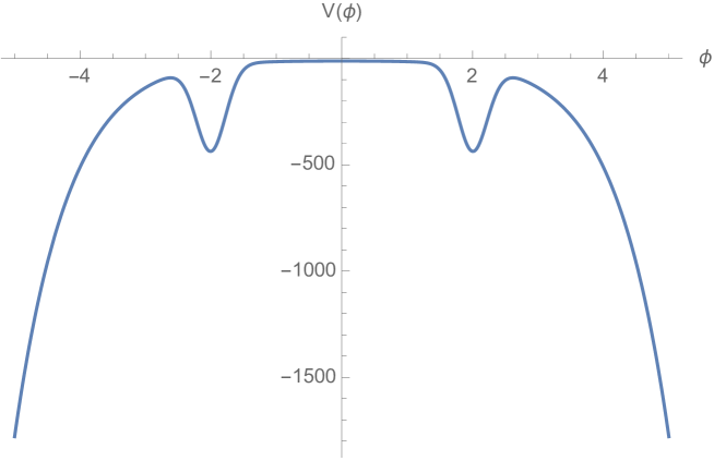
Figure 18: Example of a dilaton potential that leads to bouncing solutions. The potential is as in equation (4.46) with a choice of parameters $d=4$, $\Delta_{-}=1.7$, $\phi_{0}=4$, $\Gamma=2/\mathchoice{{\hbox{$\displaystyle\sqrt{3\,}$}\lower 0.4pt\hbox{\vrule height=6.44444pt,depth=-5.15558pt}}}{{\hbox{$\textstyle\sqrt{3\,}$}\lower 0.4pt\hbox{\vrule height=6.44444pt,depth=-5.15558pt}}}{{\hbox{$\scriptstyle\sqrt{3\,}$}\lower 0.4pt\hbox{\vrule height=4.51111pt,depth=-3.6089pt}}}{{\hbox{$\scriptscriptstyle\sqrt{3\,}$}\lower 0.4pt\hbox{\vrule height=3.22221pt,depth=-2.57779pt}}}$, $c=400$, $\sigma=1/20$. The UV fixed point corresponds to $\phi=0$ and the IR fixed point corresponds to $\phi\approx 2.00566$.

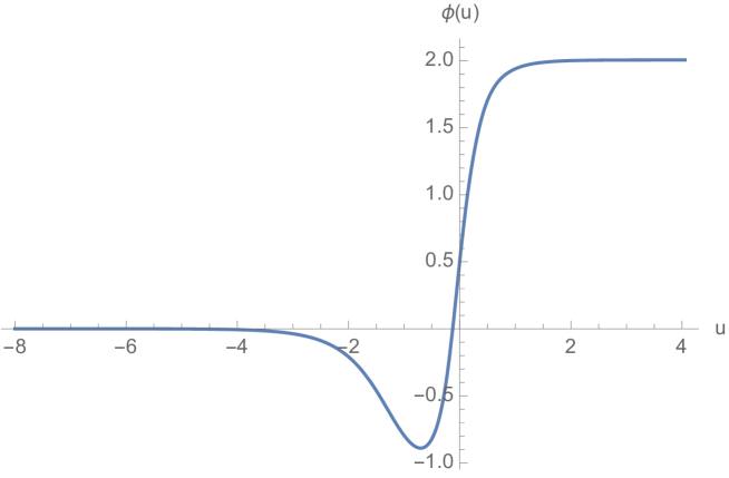
Figure 19: Bouncing zero-temperature solution for the potential shown in figure 18.

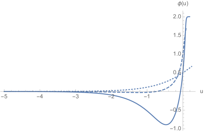
Figure 20: Comparison of the vacuum solution (solid), a bouncing finite T solution with $\phi_{h}=1.7$ (dashed) and a non-bouncing finite T solution with $\phi_{h}=0.7$ (dotted) that arise from the potential shown in figure 18.

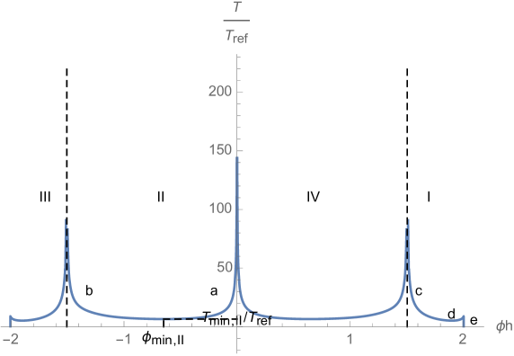
Figure 21: T as a function of $\phi_{h}$ for a particular choice of the reference scale $T_{ref}$.

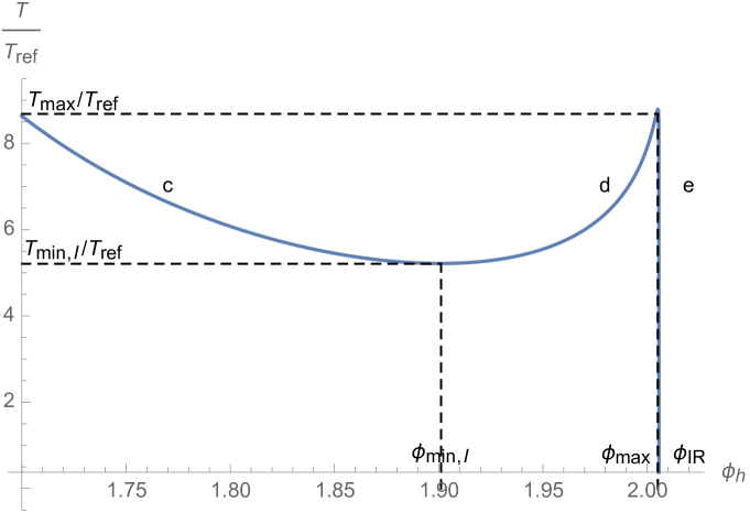
Figure 22: Blowing up the figure 21 at very small temperatures reveals existence of there different blackhole solutions for $T$ fixed between a $T_{min,I}$ and a $T_{max}$.

4.2 Bounces at finite temperature and the phase diagram

As in section 3, one has to determine $T$ as a function of $\phi_{h}$ to describe all the black-hole solutions at a given $T$. Figure 20 shows a comparison of the bouncing vacuum solution, a non-bouncing finite T solution with $\phi_{h}=0.7$ and a bouncing finite T solution with $\phi_{h}=1.7$.

Because there can be more than one $\phi_{h}$ corresponding to the same value of $T$, one needs the free energy to distinguish between these multiple black-holes and to determine the dominant one with the lowest free energy.

Calculating $T$ as a function of $\phi_{h}$ reveals the different black-hole solutions at a given temperature. This can be obtained either by constructing the geometry and using equation (2.7) or more directly from the potential using the method of scalar variables explained in appendix C, see equation (C.145). Following the latter method we obtain the function $T(\phi_{h})$ shown in figure 21.

There are four separate intervals of $\phi_{h}$ that we label from I to IV in this figure. First, we note the symmetry $T(\phi_{h})=T(-\phi_{h})$. It is not hard to see that this is an immediate consequence of the symmetry $V(\phi)=V(-\phi)$ of the dilaton potential. Moreover, there exists a critical value of $\phi_{h}$, that reads $\phi_{c}=1.507$ for the choice of parameters in figure 18, above which the black-hole solution becomes bouncing. This is demonstrated in figure 20 where we show a bouncing type black-hole for $\phi_{h}=1.7$ and a non-bouncing type for $\phi_{h}=0.7$. These two solutions belong to regions I and IV in figure 21. It is important to realise that these two regions I and IV do not belong to the same theory: as $\phi=j\,\ell^{\Delta_{-}}e^{\Delta_{-}u/\ell}+\cdots$ near the boundary, the solutions in region IV have $j>0$ whereas the solutions in region I have $j<0$ because of the bounce. Therefore the solutions in regions I and IV belong to different boundary theories.

Similarly, the solutions in region II have $j<0$ and region III have $j>0$. In the following, we will choose $|j|=1$ with no loss of generality (with this choice, the dimensionless temperature parameter ${\cal T}$ defined in equation (2.16) coincides with the temperature $T$). To simplify the presentation, we further define two reference scales $T_{ref}$ and $F_{ref}$ are defined in (C.149).

The symmetry of $V(\phi)$ under parity implies that we may only consider the solutions in regions I (bouncing) and II (non-bouncing). The physics of regions III and IV are the same except for the sign of $j$.

4.2.1 Region I: bouncing black-holes

First consider region I. As shown in figure 21, this region is further divided into three subregions, between $\phi_{c}\leq\phi_{h}<\phi_{min,I}$, $\phi_{min,I}\leq\phi_{h}<\phi_{max}$ and $\phi_{max}\leq\phi_{h}<\phi_{IR}$, labelled on the figure as “c”, “d” and “e” respectively, where for our choices of parameters we have $\phi_{min,I}=1.901$ and $\phi_{max}=2.005$. The corresponding temperatures read $T_{min,I}=5.209\,T_{ref}$ and $T_{max}=8.685\,T_{ref}$.

As clear from figure 22 there are three different black-hole solutions in this region at a given temperature between $T_{min,I}$ and $T_{max}$.

Below $T_{min,I}$ and above $T_{max}$ there is a single type of black-hole solution. The free energy of these solutions can be calculated following the method described in appendix C. The result is shown in figure 23. There is a first order phase transition at $T_{c}\approx 6T_{ref}$. This conclusion however will change once we consider the solutions in region II.

Another point to note is the free energy of the branch between $T=0$ and $T=T_{max}$, as shown figure 21 (b). The free energy of this branch is almost constant (with almost vanishing entropy) as shown in figure 23. In the limit $T\to 0$ this branch should smoothly turn into the vacuum solution. Indeed, the limiting value of the free energy as $T\to 0$ coincides precisely with the free energy of the vacuum solution.

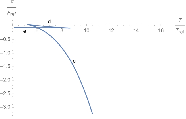
Figure 23: Free energy of bouncing type solutions in region I as a function of T that follows from the potential in figure 18. Latin letters label the different branches shown in figure 21.

4.2.2 Region II: non-bouncing black-holes

In this region there are three black-hole solutions. One observes at least two branches of solutions in figure 21, for $0\geq\phi_{h}>\phi_{min,II}$ and for $\phi_{min,II}\geq\phi_{h}>-\phi_{c}$ where $\phi_{min,II}=-0.649$. The corresponding temperature reads $T_{min,II}=6.545\,T_{ref}$.

However, there is a hidden third branch in this region, that is unveiled when one plots the entropy as a function of $T$. This is shown in figure 24 (a) and (b). Because of the shape of the function $s(T)$ near the minimum, the aforementioned second branch for $\phi_{min,II}\geq\phi_{h}>-\phi_{c}$ is further divided into two, as $T_{min,II}<T<T_{s}$ and $T_{s}<T<\infty$ where $T_{s}$ corresponds to the minimum of $s$ in figure 24 (b), with the value $T_{s}=6.560\,T_{ref}$. The corresponding value of $\phi_{h}$ is $\phi_{s}=-0.691$. Therefore, we need to divide the branch “b” in figure 21 further into two: the branch for $\phi_{min,II}\geq\phi_{h}>\phi_{s}$ and for $\phi_{s}\geq\phi_{h}>-\phi_{c}$.

The need for this further division of branches becomes more apparent upon consideration of the speed of sound in the plasma. The speed of sound can be expressed in terms of entropy and temperature as

$$c_{s}^{2}=\frac{s}{T\frac{ds}{dT}}\,.$$ (4.47)

As $s$ and $T$ are positive definite everywhere, and that $dS/dT$ vanishes (diverges) at $T=T_{s}$ ($T=T_{min,II}$) one finds that $c_{s}^{2}$ ranges between $0^{-}$ and $-\infty$ between $T_{min,II}<T<T_{s}$. The reason that $c_{s}^{2}\to-\infty$ as $\phi_{h}\to\phi_{s}^{+}$ is because $ds/dT\to 0^{-}$ there. On the other hand $c_{s}^{2}\to+\infty$ as $\phi_{h}\to\phi_{s}^{-}$, thus $c_{s}^{2}$ of this solution jumps by an infinite amount at $T=T_{s}$. Therefore one has to characterise the solutions for $T<T_{s}$ and $T>T_{s}$ differently. That $ds/dT<0$ between $T_{min,II}<T<T_{s}$ implies that this branch is thermodynamically unstable: it has negative definite specific heat per unit volume $C_{v}=Tds/dT$.

To complete the discussion of the speed of sound, we find that $c_{s}^{2}$ ranges between $1/3$ and $0^{+}$ in branch “a” on figure 21 with $0\geq\phi_{h}>\phi_{min,II}$ and it ranges between $+\infty$ and some positive value (which should be determined by precise numerics near $-\phi_{c}$) in the branch with $\phi_{s}\geq\phi_{h}>-\phi_{c}$. The fact that the speed of sound can exceed 1 in this branch most probably means that this branch is dynamically unstable, in analogy with the example studied in Gursoy:2016ggq .

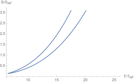
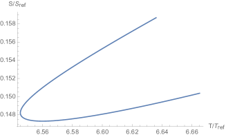
(a)                                                                       (b)

Figure 24: (a) S as a function of $T$ in region II. (b) Blow up of the figure around the minimum of $S$.

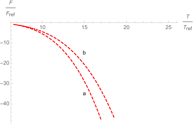
Figure 25: Free energy of non-bouncing type solutions in region II as a function of T that follows from the potential in figure 18. Latin letters label the different branches shown in figure 21.

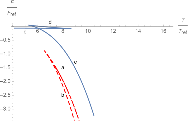
Figure 26: Comparison of the free energies of the solutions that belong to region I (blue, solid) and II (red, dashed).

Comparison of the free energies of the blackhole branches that belong to region I and II are shown in figure 26. One observes that the solutions in region II are always dominant. We observe that , as $T$ is increased first there is a first order transition between the blackhole branches “e” and “c” in region II at $T_{c}/T_{ref}=6.1$ and then there seems to be a jump in the free energy at $T=T_{min,II}=6.545T_{ref}$ from branch ”c” to branch ”b”. This jump in the free energy may indicate that the finite temperature extension of bouncing holographic RG flows is ill defined.

Finally in figure 27 we plot and compare the vacuum expectation values of the scalar operator $\langle{\cal O}\rangle$ on the blackhole branches in regions I and II.

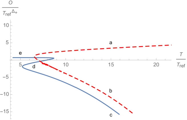
Figure 27: Comparison of the VeVs of the scalar operator on the various black hole branches in region I (blue, solid) and region II (red, dashed). Latin letters label the separate branches shown in figure 21.

5 Sourceless black holes

As we have seen in the previous two sections, there are some special values of the horizon position in field space, $\phi_{h}$, which correspond to singular limits:

• Approaching the values $\phi_{c}$ which separates between bouncing and non-bouncing solutions, the dimensionless thermodynamic quantities diverge;

• In the case considered in section 2, there is a special point $\phi_{*}$ where (at fixed source) the temperature goes to zero, though this value does not obviously correspond to the endpoint of any vacuum RG flow.

In this section we clarify the meaning of these special points. As we will see, they are new families of solutions, which correspond to flows driven by the vev of a relevant (in the case of $\phi_{c}$) or an irrelevant (in the case of $\phi_{*}$) operator. Finally, we will analyse the fate, at finite temperature, of solutions in special (fine-tuned) theories which at $T=0$ admit regular sourceless flows from a minimum to a minimum of the bulk potential, an example of which was presented in multibranch .

5.1 Thermodynamics of vev-driven flows

It is useful to analyse vev-driven flows in terms of the superpotential formalism developed in Appendix A. In this language, a sourceless flow is a solution of the first order equations governed by the superpotential of the type $W^{+}$, of the form given in equation (2.22),

$$\dot{A}=-{1\over 2(d-1)}W^{+}(\phi),\quad\dot{\phi}={dW^{+}\over d\phi}.$$ (5.48)

Unlike $W^{-}$, which contains the vev-related constant $C(\phi_{h})$ as an integration constant (see equation (2.20)), the $W^{+}$ solution is unique and does not admit continuous deformations. Therefore the solution, when expressed in terms of the scalar field as an independent variable in the superpotential formalism, is completely fixed, including the horizon position. The integration constant of the first order equation, $\phi_{+}$, is the only remaining integration constant of the solution, (recall that the integration constant in $A$ is fixed by the requirement that the boundary metric is $\eta_{\mu\nu}$ without any scaling factor). Therefore, vev-driven flows form a one-parameter family of solutions, parametrised by either $T$ or $\phi_{+}$. This is to be contrasted with source-driven flows, which are parametrised by the two independent data $(T,\phi_{-})$.

To make this more explicit, we can now repeat the scaling argument of section A.4, which shows that solutions with different values of $\phi_{+}$ are generated by the transformation

$$\phi_{+}\to e^{\Delta_{+}v}\phi_{+},\qquad T\to Te^{v},$$ (5.49)

which is the analog of the symmetry (A.97-A.99) in the case of non-zero source. This transformation leaves $\phi_{+}/T^{\Delta_{+}}$ invariant, therefore this quantity must have the same value for all vev-driven flows. We conclude that, for vev-driven black holes attached to the same UV fixed point, the vev and the temperature are not independent parameters but they must obey

$$\langle O\rangle=\overline{{\cal O}}\,T^{\Delta_{+}}$$ (5.50)

where $\overline{{\cal O}}$ is a fixed, temperature-independent, dimensionless constant.

Finally, it is useful to repeat the calculation of the free energy in the case of sourceless flows. The calculation follows the same steps detailed in Appendix B, except that instead of the solution $W^{-}$ (equation (2.20) we have to use the superpotential of the type $W^{+}$ given in equation (2.22). The crucial difference in this case is the absence of the $C\phi^{d/\Delta_{-}}$, which contributed the second term in the free energy (2.25): in this case there is no finite term coming from the sub-leading non-analytic part of the superpotential.

Therefore, for sourceless flows governed by the superpotential $W^{+}$, we simply have

$${\cal F}_{vev}=-{Ts\over d}\,V_{d-1}.$$ (5.51)

This implies that vev-driven flows have conformal thermodynamics: integrating the relation $s=-(1/V_{d-1})\partial{\cal F}/\partial T$ gives

$$s=\overline{\sigma}\,T^{(d-1)},\qquad{\cal F}_{vev}=-{\overline{\sigma}\over d}\,V_{d-1}\,T^{d}\,,$$ (5.52)

where $\overline{\sigma}$ is a fixed constant which only depends on the details of the bulk potential.

The fact that sourceless black holes display conformal thermodynamics is expected since, for zero source, conformal invariance is always softly broken. An alternative derivation of this result, based on the effective potential, will be presented in the next subsection.

5.2 Relevant vev flows

First, we consider the black holes for which the dimensionless temperature (defined in (2.16), ${\cal T}\to\infty$ as the horizon approaches a critical value $\phi_{c}$, which is in between extrema of the potential. As explained in the previous sections, the value $\phi_{c}$ separates between bouncing and non-bouncing solutions, which have opposite values of the source. This change of sign of the source is perceived as a divergence in the dimensionless temperature ${\cal T}$, which can be interpreted in two different ways depending how we approach $\phi_{c}$ in the $(T,\phi_{-})$ space:

1. If we consider the theory with fixed, finite source, then none of the solutions can have a horizon at $\phi_{h}=\phi_{c}$. As we approach this limit, the temperature $T\to\infty$ and so do the entropy and the free energy. There is no regular solution in this limit.

2. On the other hand, we can approach the $\phi_{h}=\phi_{c}$ by keeping $T$ fixed and sending $\phi_{-}\to 0$. Then we obtain regular black-hole solutions with finite free energy, a horizon exactly at $\phi_{c}$, and zero source. For these black holes, the flow is driven instead by the vev of the (relevant) operator dual to $\phi$.

In the rest of this subsection, we will examine further these critical black-hole solutions with horizon at $\phi_{c}$.

We start by noting that the limit in which the flow becomes vev-driven corresponds to the following scaling limit in the parameters entering the solution (see equation (2.21))

$$\phi_{-}\to 0,\quad C\to+\infty,\quad{d\over\Delta_{-}}{C|\phi_{-}|^{\Delta_{+}/\Delta_{-}}\over(d-2\Delta_{-})}sign(\phi_{-})=\phi_{+}^{c}\;\;\text{fixed}$$ (5.53)

In this limit, the vev $\langle O\rangle=(d-2\Delta_{-})\phi_{+}^{c}$ remains finite. As we will see shortly, the value $\phi_{+}^{c}$ is not free but it is determined by the temperature.

The most transparent way to understand the thermodynamics of the vev-driven solutions ending at $\phi_{c}$ is to use the effective potential derived in section 2.5. From equations (2.33) and (2.35), we see that solutions with $\phi_{-}=0$ correspond to extrema of the effective potential (2.35), for which

$${\cal V}^{\prime}({\cal O})=0\qquad\Rightarrow\qquad{\cal O}={\cal O}^{c}$$ (5.54)

where ${\cal O}={\langle}O{\rangle}/T^{\Delta_{+}}$ and ${\cal O}^{c}$ is a constant. This equation therefore fixes the vev in terms of the temperature,

$${\langle}O{\rangle}={\cal O}^{c}\,T^{\Delta_{+}}$$ (5.55)

Therefore, there is a one-parameter family of black holes, parametrised by $T$, all having a horizon at $\phi=\phi_{c}$, zero source, and vev given by equation (5.55).

On-shell, since the source is zero, the effective potential is the same as the free energy, and both are given by

$${\cal F}=V_{eff}(T,{\cal O}^{c})={\cal V}_{c}\,T^{d}$$ (5.56)

where ${\cal V}_{c}={\cal V}({\cal O}^{c})$ is a temperature-independent constant. We have recovered the general fact, discussed in subsection 5.1, that this family of black holes displays conformal thermodynamics, equation (5.52). Comparing equation (5.56) with (5.52) we can read-off

$${\cal V}_{c}=-{\sigma^{c}\over d}V_{d-1}$$ (5.57)

where $\sigma^{c}$ is the (fixed) ratio $s/T^{d-1}$.

Notice that, for fixed $T$ and $j=0$, the theory has another black hole solution with the same UV asymptotics: it is the AdS-Schwarzschild black hole with constant scalar field $\phi=\phi_{UV}$, sitting at the maximum of the potential. This solution also has conformal thermodynamics, with

$${\cal F}_{AdSS}=-{\sigma_{conf}\over d}\,V_{d-1}T^{d},\qquad\sigma_{conf}={(4\pi)^{d}\over d^{d-1}}(M_{p}\ell_{UV})^{d-1}$$ (5.58)

where we have expressed $\sigma_{conf}$ using equation (2.9). The question then arises, which of these two solutions is thermodynamically favored. Because of the simple scaling behaviour of the free energy, the answer is the same at all $T\neq 0$, and it boils down to comparing the values of $\sigma_{conf}$ and $\sigma^{c}$. A numerical computation shows that, in the particular models we considered here, $\sigma^{c}<\sigma_{conf}$, meaning that the AdS-Schwarzshild solution is the dominant one. For relevant vev flows ending at $\phi_{c}$ in the model in section 3, we find $\sigma^{c}=0.95\sigma_{conf}$; we come to the same conclusion for the corresponding solutions solutions in the model considered in section 4, where we find $\sigma_{c}=0.635\sigma_{conf}$.

Finally, we can go slightly off-shell and analyse the behaviour of the effective potential around the critical value ${\cal O}^{c}$. Using the scaling property (5.53) it is easy to show that, as ${\cal T}\to\infty$, the quantities $\gamma({\cal T})$ and $\sigma({\cal T})$ in equation (2.31) behave as

$$\sigma({\cal T})\to\sigma^{c},\qquad\gamma({\cal T})\simeq{\cal T}^{-\Delta_{-}}\to 0.$$ (5.59)

Performing the Legendre transform of equation (2.30) explicitly close to $\phi_{-}=0$ we find, as ${\cal O}\to{\cal O}^{c}$,

$${\cal T}\simeq-{k\over{\cal O}-{\cal O}^{c}},\quad{\cal V}({\cal O})\simeq{\cal V}_{c}+{|{\cal O}-{\cal O}^{c}|^{\Delta_{-}+1}\over(\Delta_{-}+1)k^{\Delta_{-}}},$$ (5.60)

where $k$ is a constant.

5.3 Fake zero-$T$ vacua and irrelevant flows

We now turn to another kind of special flows, which correspond to black holes ending at the point $\phi_{*}$ found in section 3 and represented in figure 17. As we have explained at the end of section 3, these black holes correspond to flows starting from the point IR₁, located at $\phi=\phi_{0}$ in figure 17, which in this case plays the role of a UV fixed point.

Since the UV is at a minimum of the potential, the conformal dimension of the deforming operator is $\Delta_{+}>d$, the operator is irrelevant, and a source term is not allowed. Therefore, the solutions with horizon at $\phi_{*}$ are driven by a vev, as those discussed in the previous section. This is consistent with the fact that, if we start from the UV at $\phi_{0}$, there is a unique value $\phi_{*}$ the scalar can take at the horizon: it is fixed by the unique solution $W^{+}$ starting at $\phi=\phi_{0}$.

By the general discussion at the beginning of this section, there is a one-parameter family of black holes, labeled by the temperature $T$, for which the vev given by

$$\langle O\rangle={\cal O}^{*}T^{\Delta_{+}},$$ (5.61)

where ${\cal O}^{*}$ is a constant.

The free energy is given by the conformal result

$${\cal F}=-{\sigma^{*}\over d}V_{d-1}\,T^{d}$$ (5.62)

where $\sigma^{*}=s/T^{(d-1)}$ is temperature-independent

Notice that the free energy is defined by renormalising with respect to IR₂, i.e. the counter-term must be chosen to be

$$S_{ct}=M_{p}^{d-1}\int d^{d}x\,\mathchoice{{\hbox{$\displaystyle\sqrt{g\,}$}\lower 0.4pt\hbox{\vrule height=4.30554pt,depth=-3.44446pt}}}{{\hbox{$\textstyle\sqrt{g\,}$}\lower 0.4pt\hbox{\vrule height=4.30554pt,depth=-3.44446pt}}}{{\hbox{$\scriptstyle\sqrt{g\,}$}\lower 0.4pt\hbox{\vrule height=3.01389pt,depth=-2.41113pt}}}{{\hbox{$\scriptscriptstyle\sqrt{g\,}$}\lower 0.4pt\hbox{\vrule height=2.15277pt,depth=-1.72223pt}}}{2(d-1)\over\ell^{2}(\phi_{0})},\quad\ell(\phi_{0})\equiv\mathchoice{{\hbox{$\displaystyle\sqrt{-{d(d-1)\over V(\phi_{0})}\,}$}\lower 0.4pt\hbox{\vrule height=15.0pt,depth=-12.00005pt}}}{{\hbox{$\textstyle\sqrt{-{d(d-1)\over V(\phi_{0})}\,}$}\lower 0.4pt\hbox{\vrule height=10.5pt,depth=-8.40004pt}}}{{\hbox{$\scriptstyle\sqrt{-{d(d-1)\over V(\phi_{0})}\,}$}\lower 0.4pt\hbox{\vrule height=7.51944pt,depth=-6.01558pt}}}{{\hbox{$\scriptscriptstyle\sqrt{-{d(d-1)\over V(\phi_{0})}\,}$}\lower 0.4pt\hbox{\vrule height=7.51944pt,depth=-6.01558pt}}}.$$ (5.63)

Since they have a different UV boundary condition (and different counter-terms) than those connecting to either UV₁ or UV₂, the black holes ending at $\phi_{*}$ belong to a boundary theory different from the ones considered in section 3 and in the previous subsection. Therefore, unlike the case considered in the previous section, we cannot describe the free energy in terms of an effective potential at criticality, since there is no well-defined conjugate variable to ${\cal O}$ which we can use to define a Legendre transform.

It is instructive to understand why these solutions seem to arise as a zero-temperature limit. As we have seen in section 3, when measuring the temperature as defined in UV₁ or UV₂, the free energy receives a vanishing contribution from the part of the solution which connects $\phi_{0}$ to $\phi_{*}$, and the limit $\phi\to\phi_{*}$ looks like a zero-temperature limit. This is due to the fact that, from the point of view of, say, UV₁, any solution starting from IR₁ is seen as describing the far infrared. Therefore, any finite temperature as measured in units of IR₁ will be rescaled to zero in units of UV₁.

Notice that there is no sense in “glueing together” the two solutions composed of the flow from 0 to $\phi_{0}$ and the flow to $\phi_{0}$ to $\phi_{*}$ to obtain a new, exotic, zero-temperature solution: indeed, the vev-driven solution from $\phi_{0}$ to $\phi_{*}$ reaches an asymptotically AdS UV boundary as $\phi\to\phi_{0}$, where $e^{A}\to+\infty$. This geometry is locally geodesically complete, and it cannot be glued across the horizon of the flow reaching $\phi_{0}$ in the IR (where $e^{A}\to 0$).

Finally, a numerical computation of $\sigma^{*}$ shows that, also in this case, the free energy (5.62) is larger than the free energy of the AdS-Schwarzschild solution of the same temperature and constant scalar field $\phi=\phi_{0}$. The latter is therefore the dominant solution at any temperature for $j=0$.

5.4 Minimum-to-minimum irrelevant flows

In this section, we consider the finite-temperature generalisation of the flows connecting two minima of the potential (one serving as a UV fixed point, the other as an IR fixed point). These flows, discussed in multibranch , are driven by the vev of an irrelevant operator, in contrast to the zero-temperature solutions discussed in the sections 3 and 4, for which the operator was always relevant. They are shown schematically in terms of the associated superpotential in figure 28.

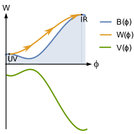
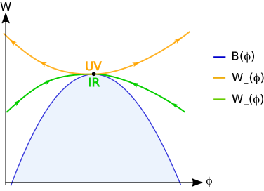
(a)                                                      (b)

Figure 28: A minimum to minimum flow is displayed. The left figure (a) shows a schematic picture of the superpotential (yellow curve) and the bulk potential (green curve). The curve $B(\phi)$ is defined via equation (A.86) and is the boundary of the forbidden region below which the zero-temperature superpotential cannot go. The right figure (b) shows a sketch of solutions of the superpotential equation with critical point at a local minimum of the potential (local maximum of $B(\phi)$). The $W_{+}(\phi)$ and $W_{-}(\phi)$ solutions correspond each to two asymptotically AdS geometries in the UV and IR, respectively. The corresponding geometries are not connected, as each flow stops (or starts) at the fixed point. The arrows on $W_{-}(\phi)$ and $W_{+}(\phi)$ indicate the direction of the holographic RG flow.

As we discuss below, at zero temperature, these theories display a moduli space of vacua. We will see that this is lifted when temperature is turned on, and that the only point in the moduli space that is left is the AdS black hole with constant scalar field profile.

Minimum-to-minimum flows are interesting because they provide the only regular zero-temperature flows in this setup which are driven by the vacuum expectation value of an irrelevant operator. Such flows arise from spontaneous breaking of scale invariance of the boundary theory: the source $J$ of the UV theory operator $O$ is zero as it is non-renormalisable and, yet, this operator acquires a non-zero VEV which is related to the asymptotic behaviour of $\phi(u)$ through

$$\phi(u)=\phi_{+}\,\ell^{\Delta_{+}}e^{\Delta_{+}u}+\ldots,\qquad\langle O\rangle=\left(M_{p}\ell\right)^{d-1}(d-2\Delta_{-})\phi_{+}\,.$$ (5.64)

Equation (5.64) is valid for both zero and finite temperature. For generic potentials and at zero temperature, the bulk geometries in the class (5.64) are singular. However, for special potentials, it is possible to make the flow reach a second minimum of $V$ in the IR, providing a regular solution with IR AdS asymptotics multibranch .

The first-order or superpotential formalism of appendix A provides a single description of all zero-temperature flows of the form (5.64) as well as an easy implementation of the regularity condition. The flows of the form (5.64) with non-zero $\left<O\right>$ which start from a given minimum of $V$ (seen as a UV fixed point) are associated with a unique superpotential of the type $W^{+}(\phi)$, with an asymptotic expansion of the form (2.22). This is the yellow curve in figure 28 (b)), where, for comparison, we also displayed the $W_{-}$-type solution arriving at the same minimum for which this point is seen as an IR fixed point.The blue curve in figure 28, $B(\phi)$, is defined though equation (A.86) and it is the lower bound on $W$ at zero temperature: the shaded blue region is not allowed, as a consequence of the superpotential equation (A.70) with $f\equiv 1$ (see appendix A.2 for more details).

At $T=0$, these models display a moduli space of vacua, parametrised by $\phi_{+}$. The reason is that the superpotential which describes these flows is of the type $W^{+}$ which, as we explained in subsection 5.1, does not contribute a finite part $\sim C\phi^{d/\Delta_{-}}$ to the renormalised on-shell action. Equation (2.29) then implies that the zero-temperature free energy ${\cal F}=0$ for any value $\left<O\right>$.

This one-parameter degeneracy of vacua is continuously connected to the AdS vacuum of the unbroken theory, which corresponds to $\left<O\right>=0$ and to a constant scalar field profile and also has vanishing free energy.

At finite temperature, as we have seen in subsection (5.1), we generically expect for vev-driven black holes a relation between $\langle O\rangle$ and $T$ of the form (5.55). This means that at any fixed temperature at most one solution is expected, and the moduli space is lifted. Moreover, taking the $T\to 0$ limit we only obtain an AdS solution with $\langle O\rangle=0$ i.e. these black holes, if they exist, are connected only to the constant-$\phi$ solution and to no other solution in the moduli space.

The previous considerations suggest that the solutions with non-zero $\langle O\rangle$ and non-trivial scalar field profile do not have any finite-temperature generalisation: to obtain a finite $\langle O\rangle$ at $T=0$ one would need the constant $\overline{\cal O}$ in equation (5.50) to be infinite, in which case the finite temperature VEV would diverge. Since the $W^{+}$-type potential admits no continuous deformations close to the UV wenliang ; multibranch , there cannot be regular black holes with $\langle O\rangle=0$ starting from the same UV minimum as the zero-temperature regular flow. The reason is that there exists a $W^{+}$ regular solution for $f=1$ and therefore any other regular solution with non-trivial $f$ will “miss” the UV fixed point and flow somewhere else.

We will now move to a concrete example in which we find that these expectations are correct: in the theory that admits a regular minimum-to-minimum flow at $T=0$, there are no black-hole solutions which start from the same UV.

To be concrete, we consider the model presented in reference multibranch , which we will subsequently study at finite temperature. In $d$ boundary dimensions, the following family of superpotentials parametrised by $k$, $v$ and $W_{*}$,

$$W(\phi)=kv^{2}\left(\phi\over v\right)\left[1-{1\over 3}\left(\phi\over v\right)^{2}\right]+W_{*}$$ (5.65)

allows for very simple kink scalar field profiles:

$$\phi(u)=v\tanh(k~{}(u-u_{*}))~{}.$$ (5.66)

Each superpotential in (5.65) solves (A.70) with $f(\phi)=1$ and with the potential

$$V(\phi)={(kv)^{2}\over 2}\left[1-\left(\phi\over v\right)^{2}\right]^{2}-\frac{d}{4(d-1)}\left\{kv^{2}\left(\phi\over v\right)\left[1-{1\over 3}\left(\phi\over v\right)^{2}\right]+W_{*}\right\}^{2}~{}.$$ (5.67)

The flows of the form (5.66) interpolate between the extrema of $V(\phi)$ at $\phi=-v$ and $\phi=v$. A region of parameter space which includes the point

$$v=k=1,~{}~{}d=4~{}~{}{\text{and}}~{}~{}W_{*}=1.8$$ (5.68)

is such that the extrema of $V(\phi)$ at $\phi=\pm v$ are both local minima. The potential (5.67) is not everywhere negative, however it is negative between $-v$ and $v$ for the values (5.68) of the parameters. As we argued in multibranch , the sign of $V(\phi)$ outside the range of definition of a superpotential $W(\phi)$ does not affect the existence of this kind of flow because the equations of motion are local in field space. In this particular model, the maximum of $V$ in between the two minima violates the BF bound, so it does not provide a consistent UV for the theory. This is inconsequential as far as the minimum-to-minimum flow is concerned.

At finite temperature, we need to solve the system (A.70- A.71). Contrary to the zero-temperature case where the bound (A.86) holds as long as the potential is strictly negative, at finite temperature even strictly negative potentials allow a positive $W(\phi)$ to cross into the forbidden region and to be arbitrarily small, as follows for example from equation (A.87).

To scan for black-hole solution numerically, we choose a set of values of horizon position $\phi_{h}$ in the interval $(-v,v)$ and and solve numerically the system (A.70- A.71) providing boundary conditions at $\phi_{h}+\delta\phi$ using the relations (A.76). What we find is that no solution reaches the would be UV point $\phi=-v$, but all of them bounce at some larger $\phi$. The resulting superpotentials are displayed in figure 29, where only the branch above the bound is displayed and we set $v=1$. The closer the horizon position $\phi_{h}$ is to $\phi=v$, the larger $W$ and the closer the bounce is to $\phi=-1$. No finite-temperature solution reaches $\phi=-1$, no matter how close to $v=1$ we set the horizon. This is further emphasised in figures 30 and 31 which display $W^{\prime}(\phi)$ for different values of $\phi_{h}$.

\begin{overpic}[width=303.53267pt]{Figures/WTbis} \end{overpic}

Figure 29: The blue curve bounding the shaded region represents the curve $B(\phi)$ which bounds superpotentials at zero temperature (see (A.86)). It is presented here to locate the extrema of the potential between which the zero temperature solution flows. The green curve which starts at -1 with value $B(-1)$ and extends until $\phi=1$ where its value is $B(1)$ corresponds to the zero-temperature solution. The remaining curves correspond to finite-temperature superpotentials solving (A.70) and (A.71) with boundary conditions (A.76-A.77) for the potential (5.67-5.68). The values of $W$ increase as the horizon position takes values closer and closer to the IR extremum at $\phi=v$. None of the black-hole solutions reach the local minimum of $V$ at $\phi=-1$, they all bounce for $\phi>-1$. The position of the bounces and their progression as $\phi_{h}$ approaches $v$ is clearer when looking at $W^{\prime}(\phi)$, as is done in figures 30 and 31.

\begin{overpic}[width=303.53267pt]{Figures/dWTbis} \end{overpic}

Figure 30: This figure shows the first derivative of the functions displayed in figure 30. The curve which extends from $-1$ to $1$ corresponds to the zero-temperature solution. The remaining curves are the derivatives with respect to $\phi$ of the finite-temperature superpotentials displayed in figure 29. The rightmost zero (or the tendance of $W^{\prime}$ to vanish) corresponds to the horizon position which approaches $\phi=1$ without reaching it and the leftmost zero corresponds to the bounce position. The closer the horizon is to $\phi=1$ the closer the bounce gets to $\phi=-1$ but the superpotential never reaches $-1$. This means that the zero-temperature minimum-to-minimum flow is not associated with a black hole. The bouncing points are better visualised in figure 31.

\begin{overpic}[width=303.53267pt]{Figures/dWT2bis} \end{overpic}

Figure 31: A closer look at the near-bounce region of figure 30. The leftmost curve corresponds to the zero temperature solution and the remaining curves are superpotentials at finite temperature. The derivative of each finite-temperature superpotential vanishes at a different bouncing point, where the each solution is glued to the next branch. The closer to $-1$ the zero of $dW/d\phi$ is, closer the horizon is to $\phi=1$ and lower is the black-hole temperature. No finite-temperature solution reaches $\phi=-1$, thus showing that the minimum-to-minimum zero temperature flow from multibranch does not have an associated black-hole solution with a running scalar.

The conclusion is that all the black holes in this model miss the UV minimum at $v=-1$ and flow towards the intermediate maximum. The latter however violates the BF bound, so these states are not part of healthy theory. A part from this, conceptually they are in the same class as the black holes with UV asymptotics at a maximum of $V$, which were discussed in the previous sections.

Appendices

Appendix A First order formalism

As for the zero-temperature solutions, we can introduce a function $W(\phi)$ such that, on-shell

$$\dot{A}(u)=-{1\over 2(d-1)}W(\phi(u)),\quad\dot{\phi}(u)={dW(\phi(u))\over d\phi}$$ (A.69)

This can always be achieved piecewise in any region where $\phi(u)$ is monotonic, by inverting the relation $\phi(u)\to u(\phi)$. With the definition (A.69) equation (2.5d) is identically satisfied, and the remaining equations (2.5a-2.5c) become a system of scalar equations for the functions $W(\phi)$, $f(\phi)\equiv f(u(\phi))$ KN ,

$$\left({1\over 2}\left({dW\over d\phi}\right)^{2}-\frac{d}{4(d-1)}W^{2}\right)f+{W\over 2}\frac{df}{d\phi}{dW\over d\phi}=V~{},$$ (A.70)

$${d^{2}f\over d\phi^{2}}{dW\over d\phi}+{df\over d\phi}{d^{2}W\over d\phi^{2}}-{d\over 2(d-1)}W{df\over d\phi}=0.$$ (A.71)

For $f(\phi)=1$ , equation (A.70) becomes the usual superpotential equation.

Among the transformations 2.6 which leave the original equations of motion invariant, only (2.6c) affects (A.70) and (A.71). The corresponding transformations for $W(\phi)$ and $f(\phi)$ are

$$\left(\tilde{f}(\phi),\tilde{W}(\phi)\right)\to\Big{(}f(\phi),W(\phi)\Big{)}=\Big{(}\lambda^{2}\tilde{f}\left(\phi\right),\lambda^{-1}\tilde{W}\left(\phi\right)\Big{)}$$ (A.72)

and $\phi$ is left invariant.

A.1 The integration constants for the superpotential equations

The system (A.70-A.71) is third order and can be solved in terms of three integration constants which can be chosen in different ways. It is most convenient to view it as a boundary value problem for $f(\phi)$ and an initial value problem (at the black-hole horizon) for $W(\phi)$, and fix the integration constants by

$$f(0)=1,\qquad f(\phi_{h})=0,\qquad W(\phi_{h})=W_{h}.$$ (A.73)

The first equation follows from the requirement that the leading asymptotic boundary metric is the same for all solutions. This leaves the two arbitrary parameters parameters $\phi_{h}$ and $W_{h}$. As we will show below however, $W_{h}$ is also fixed uniquely by the choice the horizon position $\phi_{h}$, resulting in a one-parameter family of solutions parametrised by the value of $\phi_{h}$.

A very simple way to see that the system (A.70- A.71) is third order and which is helpful to give boundary conditions for solving the system numerically goes as follows. By differentiating equation (A.70) with respect to $\phi$, a term with $f^{\prime\prime}(\phi)$ is generated and can be used to eliminate $f^{\prime\prime}(\phi)$ from (A.71). The resulting equation is:

$$W^{\prime}(\phi)\left[f(\phi)\left(\frac{dW(\phi)}{2-2d}+W^{\prime\prime}(\phi)\right)+f^{\prime}(\phi)W^{\prime}(\phi)\right]=V^{\prime}(\phi),$$ (A.74)

Equations (A.70) and (A.74) demand three integration constants which completely specify $W(\phi)$ and $f(\phi)$. Evaluating (A.70) and (A.74) at the horizon we obtain

$$\left[{W}{f^{\prime}}{W^{\prime}}\right]_{\phi_{h}}=2V(\phi_{h}),$$ (A.75a)

$$\left[W^{\prime}f^{\prime}W^{\prime}\right]_{\phi_{h}}=V^{\prime}(\phi_{h})~{}.$$ (A.75b)

For any choice of the integration constant $f^{\prime}(\phi_{h})$ and imposing that $W$ is positive, the system (A.75) completely specifies $W(\phi_{h})$ and $W^{\prime}(\phi_{h})$. Therefore one can chose boundary conditions close to the horizon as follows:

$$f(\phi_{h}+\delta\phi)=\delta\phi~{}f^{\prime}(\phi_{h})+{\cal O}(\delta\phi^{2})\qquad\text{with}\quad f^{\prime}(\phi_{h})\delta\phi>0,$$ (A.76a)

$$W^{\prime}(\phi_{h}+\delta\phi)=\mathchoice{{\hbox{$\displaystyle\sqrt{\frac{V^{\prime}(\phi_{h})}{f^{\prime}(\phi_{h})}\,}$}\lower 0.4pt\hbox{\vrule height=16.38887pt,depth=-13.11116pt}}}{{\hbox{$\textstyle\sqrt{\frac{V^{\prime}(\phi_{h})}{f^{\prime}(\phi_{h})}\,}$}\lower 0.4pt\hbox{\vrule height=11.50554pt,depth=-9.20447pt}}}{{\hbox{$\scriptstyle\sqrt{\frac{V^{\prime}(\phi_{h})}{f^{\prime}(\phi_{h})}\,}$}\lower 0.4pt\hbox{\vrule height=8.90276pt,depth=-7.12224pt}}}{{\hbox{$\scriptscriptstyle\sqrt{\frac{V^{\prime}(\phi_{h})}{f^{\prime}(\phi_{h})}\,}$}\lower 0.4pt\hbox{\vrule height=8.90276pt,depth=-7.12224pt}}}+{\cal O}(\delta\phi)~{},$$ (A.76b)

$$W(\phi_{h}+\delta\phi)=-\frac{2V(\phi_{h})}{\mathchoice{{\hbox{$\displaystyle\sqrt{f^{\prime}(\phi_{h})V^{\prime}(\phi_{h})\,}$}\lower 0.4pt\hbox{\vrule height=8.5pt,depth=-6.80003pt}}}{{\hbox{$\textstyle\sqrt{f^{\prime}(\phi_{h})V^{\prime}(\phi_{h})\,}$}\lower 0.4pt\hbox{\vrule height=8.5pt,depth=-6.80003pt}}}{{\hbox{$\scriptstyle\sqrt{f^{\prime}(\phi_{h})V^{\prime}(\phi_{h})\,}$}\lower 0.4pt\hbox{\vrule height=5.97221pt,depth=-4.7778pt}}}{{\hbox{$\scriptscriptstyle\sqrt{f^{\prime}(\phi_{h})V^{\prime}(\phi_{h})\,}$}\lower 0.4pt\hbox{\vrule height=4.58333pt,depth=-3.66669pt}}}}+\delta\phi\mathchoice{{\hbox{$\displaystyle\sqrt{\frac{V^{\prime}(\phi_{h})}{f^{\prime}(\phi_{h})}\,}$}\lower 0.4pt\hbox{\vrule height=16.38887pt,depth=-13.11116pt}}}{{\hbox{$\textstyle\sqrt{\frac{V^{\prime}(\phi_{h})}{f^{\prime}(\phi_{h})}\,}$}\lower 0.4pt\hbox{\vrule height=11.50554pt,depth=-9.20447pt}}}{{\hbox{$\scriptstyle\sqrt{\frac{V^{\prime}(\phi_{h})}{f^{\prime}(\phi_{h})}\,}$}\lower 0.4pt\hbox{\vrule height=8.90276pt,depth=-7.12224pt}}}{{\hbox{$\scriptscriptstyle\sqrt{\frac{V^{\prime}(\phi_{h})}{f^{\prime}(\phi_{h})}\,}$}\lower 0.4pt\hbox{\vrule height=8.90276pt,depth=-7.12224pt}}}+{\cal O}(\delta\phi^{2})~{}.$$ (A.76c)

The boundary conditions (A.76) will typically lead to $f(\phi_{UV})\neq 1$, however this apparent inconvenience is immediately circumvented with a rescaling of the form (A.72) with parameter

$$\lambda=(f(\phi_{UV}))^{-1/2}~{}.$$ (A.77)

Another way to specify the integration constants is to explicitly identify the boundary theory source in $f(\phi)$ and the product $TS$ in $W(\phi)$, making a more explicit contact with the thermodynamics. To proceed, we chose a value $\phi_{h}$. First, notice that equation (A.71) can also be written equivalently as

$${d\over d\phi}\left[{df\over d\phi}{dW\over d\phi}e^{d{\cal A}(\phi)}\right]=0$$ (A.78)

where

$${\cal A}(\phi)=-{1\over 2(d-1)}\int^{\phi}d\hat{\phi}{W\over W^{\prime}}$$ (A.79)

The function ${\cal A}(\phi)$ depends on an arbitrary additive constant but clearly this does not affect equation (A.78), and in fact it can be reabsorbed in one of the other integration constants. Integrating equation (A.78) gives

$${df\over d\phi}=-{\tilde{D}\over W^{\prime}}e^{-d{\cal A}(\phi)},$$ (A.80)

where $\tilde{D}$ is a constant. As we mentioned above, an additive constant in ${\cal A}(\phi)$ can be absorbed in a redefinition of $\tilde{D}$ and we can fix this redundancy (which does not correspond to one of the integration constants of the system (A.70-A.71)) so that ${\cal A}(\phi_{h})=0$:

$$\qquad{\cal A}(\phi)=-{1\over 2(d-1)}\int_{\phi_{h}}^{\phi}d\hat{\phi}{W\over W^{\prime}}$$ (A.81)

Equation (A.80) can be further integrated to give

$$f(\phi)=\tilde{F}-\tilde{D}\int_{0}^{\phi}{dy\over W^{\prime}(y)}e^{-d{\cal A}(y)}.$$ (A.82)

As we will see in a moment, the second term vanishes as $\phi\to 0$. Therefore, imposing the boundary conditions for $f(\phi)$ from equation (A.73) fixes

$$\tilde{F}=1,\quad\tilde{D}=\left(\int_{0}^{\phi_{h}}{dy\over W^{\prime}(y)}e^{-d{\cal A}(y)}\right)^{-1}.$$ (A.83)

Finally, evaluating equation (A.70) at $\phi_{h}$ and using (A.80) we find

$$W(\phi_{h})=-{2V(\phi_{h})\over\tilde{D}}.$$ (A.84)

This condition is equivalent to the requirement that the horizon is regular, and it fixes the remaining free parameter $W_{h}$ in the initial conditions (A.73).

To summarise we have found that, for regular asymptotically $AdS$ black holes, solutions to the system (A.70-A.78) depend on a single continuous free parameter, which we can be taken to be the horizon position $\phi_{h}$. In the next subsection we will clarify the physical meaning of the quantity $\tilde{D}(\phi_{h})$.

A.2 Lower bounds on the superpotential

At zero temperature, an important property of $W(\phi)$ is that it is bounded from below. This can be shown by considering equation (A.70) with $f(\phi)\equiv 1$ and algebraically solving for $W$:

$$|W(\phi)|=\mathchoice{{\hbox{$\displaystyle\sqrt{\frac{4(d-1)}{d}\left({1\over 2}W^{\prime 2}-V(\phi)\right)\,}$}\lower 0.4pt\hbox{\vrule height=13.47221pt,depth=-10.77782pt}}}{{\hbox{$\textstyle\sqrt{\frac{4(d-1)}{d}\left({1\over 2}W^{\prime 2}-V(\phi)\right)\,}$}\lower 0.4pt\hbox{\vrule height=9.43054pt,depth=-7.54446pt}}}{{\hbox{$\scriptstyle\sqrt{\frac{4(d-1)}{d}\left({1\over 2}W^{\prime 2}-V(\phi)\right)\,}$}\lower 0.4pt\hbox{\vrule height=6.7361pt,depth=-5.3889pt}}}{{\hbox{$\scriptscriptstyle\sqrt{\frac{4(d-1)}{d}\left({1\over 2}W^{\prime 2}-V(\phi)\right)\,}$}\lower 0.4pt\hbox{\vrule height=6.7361pt,depth=-5.3889pt}}}\geqslant\mathchoice{{\hbox{$\displaystyle\sqrt{-\frac{4(d-1)}{d}V(\phi)\,}$}\lower 0.4pt\hbox{\vrule height=13.47221pt,depth=-10.77782pt}}}{{\hbox{$\textstyle\sqrt{-\frac{4(d-1)}{d}V(\phi)\,}$}\lower 0.4pt\hbox{\vrule height=9.43054pt,depth=-7.54446pt}}}{{\hbox{$\scriptstyle\sqrt{-\frac{4(d-1)}{d}V(\phi)\,}$}\lower 0.4pt\hbox{\vrule height=6.7361pt,depth=-5.3889pt}}}{{\hbox{$\scriptscriptstyle\sqrt{-\frac{4(d-1)}{d}V(\phi)\,}$}\lower 0.4pt\hbox{\vrule height=6.7361pt,depth=-5.3889pt}}}\equiv B(\phi)>0.$$ (A.85)

When $V(\phi)$ is negative, $W$ can never approach zero, meaning that the branches with $W>0$ and $W<0$ which solve (A.85) are disconnected. Furthermore, they are physically equivalent as one can pass from one to the other by the transformation $(u,W)\to(-u,-W)$. Therefore, without loss of generality we can choose a positive $W$, meaning that $\dot{A}(u)$ is negative, and see (A.85) as a lower bound on $W$ and not just on its absolute value:

$$W(\phi)\geqslant B(\phi)\equiv\mathchoice{{\hbox{$\displaystyle\sqrt{-\frac{4(d-1)}{d}V(\phi)\,}$}\lower 0.4pt\hbox{\vrule height=13.47221pt,depth=-10.77782pt}}}{{\hbox{$\textstyle\sqrt{-\frac{4(d-1)}{d}V(\phi)\,}$}\lower 0.4pt\hbox{\vrule height=9.43054pt,depth=-7.54446pt}}}{{\hbox{$\scriptstyle\sqrt{-\frac{4(d-1)}{d}V(\phi)\,}$}\lower 0.4pt\hbox{\vrule height=6.7361pt,depth=-5.3889pt}}}{{\hbox{$\scriptscriptstyle\sqrt{-\frac{4(d-1)}{d}V(\phi)\,}$}\lower 0.4pt\hbox{\vrule height=6.7361pt,depth=-5.3889pt}}}>0.$$ (A.86)

Another useful property to understand the numerical results shown in figures 29, 30 and 31 which is related to the normalisation of $f(\phi)$ is that $W$ can lie below $B(\phi)$ defined in (A.86). It is instructive to algebraically solve equation (A.70) for $W(\phi)$ keeping into account the positivity of $W$ which is necessary for $\dot{A}$ to be negative

$$W(\phi)={(d-1)\over{d}}{f^{\prime}W^{\prime}\over f}+\mathchoice{{\hbox{$\displaystyle\sqrt{{\left({(d-1)\over d}{f^{\prime}W^{\prime}\over{f}}\right)^{2}+{2(d-1)\over d}\left(W^{\prime 2}-{2V\over f}\right)}\,}$}\lower 0.4pt\hbox{\vrule height=14.88889pt,depth=-11.91116pt}}}{{\hbox{$\textstyle\sqrt{{\left({(d-1)\over d}{f^{\prime}W^{\prime}\over{f}}\right)^{2}+{2(d-1)\over d}\left(W^{\prime 2}-{2V\over f}\right)}\,}$}\lower 0.4pt\hbox{\vrule height=10.44441pt,depth=-8.35558pt}}}{{\hbox{$\scriptstyle\sqrt{{\left({(d-1)\over d}{f^{\prime}W^{\prime}\over{f}}\right)^{2}+{2(d-1)\over d}\left(W^{\prime 2}-{2V\over f}\right)}\,}$}\lower 0.4pt\hbox{\vrule height=7.77776pt,depth=-6.22223pt}}}{{\hbox{$\scriptscriptstyle\sqrt{{\left({(d-1)\over d}{f^{\prime}W^{\prime}\over{f}}\right)^{2}+{2(d-1)\over d}\left(W^{\prime 2}-{2V\over f}\right)}\,}$}\lower 0.4pt\hbox{\vrule height=7.77776pt,depth=-6.22223pt}}}$$ (A.87)

As long as $V(\phi)$ is negative, it is guaranteed that $W$ is real at stationary points, i.e. when $W^{\prime}$ vanishes. Negativity of $V(\phi)$ also guarantees that giving $W$ a positive value at any fixed $\phi=\phi_{0}$ implies the positivity of $W$ for all $\phi$. In contrast to the zero temperature case, the function $f(\phi)$ permits the existence of solutions such that the limit

$$\left({f^{\prime}W^{\prime}\over{f}}\right)^{2}\gg{2d\over d-1}\left(W^{\prime 2}-{2V\over f}\right)$$ (A.88)

holds, thus including arbitrarily small superpotentials in the space of solutions. On the other hand, from (A.87) it follows that the value of $W(\phi)$ at critical points, i.e. those where $W^{\prime}(\phi)$ vanishes, is set by $f(\phi)$ and $V(\phi)$,

$$W^{\prime}=0\quad{\text{and}}\quad{f^{\prime}W^{\prime}\over{f}}=0\qquad\implies\qquad W=\mathchoice{{\hbox{$\displaystyle\sqrt{{-{4(d-1)\over d}{V\over f}}\,}$}\lower 0.4pt\hbox{\vrule height=13.47221pt,depth=-10.77782pt}}}{{\hbox{$\textstyle\sqrt{{-{4(d-1)\over d}{V\over f}}\,}$}\lower 0.4pt\hbox{\vrule height=9.43054pt,depth=-7.54446pt}}}{{\hbox{$\scriptstyle\sqrt{{-{4(d-1)\over d}{V\over f}}\,}$}\lower 0.4pt\hbox{\vrule height=6.7361pt,depth=-5.3889pt}}}{{\hbox{$\scriptscriptstyle\sqrt{{-{4(d-1)\over d}{V\over f}}\,}$}\lower 0.4pt\hbox{\vrule height=6.7361pt,depth=-5.3889pt}}}$$ (A.89)

one of the few remaining properties from the zero temperature setup.

A.3 Near-boundary solution: universal part

To obtain the solution close to the boundary, we solve the system of equations (A.70-A.78) perturbatively close to $\phi=0$, where $f\simeq 1$. To lowest order we obtain the analytic part $W_{0}$ of the superpotential,

$$W_{0}^{\pm}(\phi)={2(d-1)\over\ell}+{{\Delta_{\pm}}\over 2\ell}\phi^{2}+O(\phi^{4}),$$ (A.90)

which coincide with the perturbative expansion in the vacuum solution, see e.g. Papadimitriou:2007sj ; wenliang ; multibranch . The two choices, $\Delta_{-}$ or $\Delta_{+}$, in the quadratic term, correspond respectively to a flow driven by a source or by a vev of the operator dual to $\phi$. Generically we will be describing flows with non-zero source, therefore from now on we will choose $W_{0}=W_{0}^{-}$. Vev-driven flows will play an important role however, and will be discussed separately later on.

Up to higher order corrections, we can replace $W$ by $W_{0}$ in ${\cal A}$ in (A.80) and close to the boundary we find

$${\cal A}(\phi)={\cal A}_{0}-{1\over\Delta_{-}}\log|\phi|+O(\phi)$$ (A.91)

where ${\cal A}_{0}$ is a constant which is also completely determined by equation (A.81) and depends only on $\phi_{h}$.

Using equations (A.90) and (A.91) we can approximate equation (A.82) for close to $\phi=0$,

$$f(\phi)=1-{\tilde{D}e^{-d{\cal A}_{0}}\ell\over d}|\phi|^{d\over\Delta_{-}}.$$ (A.92)

As announced, the $\phi-$dependent part vanishes as $\phi\to 0$, and $f$ satisfies the correct boundary condition.

Finally, integrating equations (A.69) give the expected leading order scaling,

$$A(u)=-{u\over\ell}+O(e^{u}),\qquad\phi(u)=j\,\ell^{\Delta_{-}}e^{\Delta_{-}u/\ell}+\ldots,\qquad u\to-\infty,$$ (A.93)

and introduces as additional free parameter $j$, the constant corresponding to the source of the dual operator, whose choice is part of the boundary data one has to give to fix the holographic theory. The other piece of boundary data is the leading asymptotic behaviour of the boundary metric: in writing equation (A.93) we have chosen the constant term in $A$ to vanish, so that in the holographic dictionary the dual field theory metric is $\eta_{\mu\nu}$ with unit coefficient.

Thus, the full solution $(A(u),\phi(u),f(u))$ depends on only two parameters: the value of the source $j$ and the horizon position $\phi_{h}$. The black-hole temperature and entropy density are therefore determined by these two quantities. In the next section we will make this dependence more explicit.

A.4 Dimensionless temperature and entropy

Equations (A.92-A.93) reproduce the expected scaling (2.13) near the boundary. Comparing equations (A.92) and (2.13c), and using the relation (A.80) we can relate $\tilde{D}$ to the black-hole temperature $T$ and entropy density $s$:

$$\tilde{D}e^{-d{\cal A}_{0}}={1\over M_{p}^{d-1}}\,\,{Ts\over|j|^{d/\Delta_{-}}}.$$ (A.94)

As the right hand side depends only on $\phi_{h}$, the same must be true for the combination on the right hand side. In fact we will now show that the two quantities

$${\cal T}\equiv{T\over|j|^{1/\Delta_{-}}},\qquad{\cal S}\equiv{s\over|j|^{(d-1)/\Delta_{-}}}$$ (A.95)

are function of $\phi_{h}$ only. They represent the temperature and entropy density in units of the UV source $j$.

To see that the ${\cal T}$ and ${\cal S}$ defined above depend on $\phi_{h}$ only, and not on both $\phi_{h}$ and $j$, we use the invariance property (2.6a-2.6b),

$$u\to u^{\prime}=u+v,\qquad A(u)\to A^{\prime}(u^{\prime})=A(u^{\prime})+\bar{A}.$$ (A.96)

Starting from a solution, these transformation produces a new solution of the same form (2.4) but with different UV data, temperature and entropy: the source term transforms as

$$j\to e^{\Delta_{-}v}j$$ (A.97)

and the horizon data as

$$u_{h}\to u_{h}+v,\quad e^{A(u_{h})}\to e^{A(u_{h}+v)+\bar{A}},\quad\dot{f}(u_{h})\to\dot{f}(u_{h}+v)$$ (A.98)

However if we want to keep the boundary metric fixed to be $\eta_{\mu\nu}$ we have to choose $\bar{A}=v/\ell$, as we have to cancel a constant term in the asymptotic expansion of $A(u)$, equation (A.93). Taking this into account, we find that under (A.96)

$$T\to e^{v}T,\qquad s\to e^{(d-1)v}s$$ (A.99)

On the other hand, the horizon value $\phi_{h}$ is unaffected by this transformation, so all solutions related by the transformation (A.96) have the same $\phi_{h}$ and the same values of the combinations (A.95). We conclude that both ${\cal T}$ and ${\cal S}$ are determined solely by the horizon field value $\phi_{h}$. Since ${\cal T}$ (as opposed to $\phi_{h}$) is directly related to the horizon data $(T,j$, it is useful to invert the relation ${\cal T}(\phi_{h})$ (at least piecewise) and use ${\cal T}$ to parametrise black-hole solutions with the same $\phi_{h}$.

A.5 Near-boundary solution: sub-leading term

The sub-leading, non-analytic contributions to $W(\phi)$ beyond the leading behaviour (A.90) contains the information about the vevs, see wenliang ; multibranch and gives finite contributions to the free energy. It can be obtained by setting $W=W_{0}+\delta W$, linearizing equation (A.70) around the solution (A.90) and keeping in mind that $f=1+O(\phi^{d\Delta_{-}})$. The resulting equation is

$$W_{0}^{\prime}\delta W^{\prime}-{d\over 2(d-1)}W_{0}\delta W_{0}=(f_{0}-1)V+f_{0}^{\prime}W_{0}^{\prime}W_{0}$$ (A.100)

Using the expression for $f_{0}$ in equation (A.92) and evaluating $V$ at the origin (recall $V(0)=-d(d-1)\ell^{-2}$) we find that the right hand side vanishes at the lowest order $\phi^{d/\Delta_{-}}$, and it starts at order $\phi^{d/\Delta_{-}+2}$. To lowest order the solution for $\delta W$ is

$$\delta W=\ell^{-1}C(\phi_{h})|\phi|^{d/\Delta_{-}}\left(1+O(\phi^{2})\right)$$ (A.101)

where $C(\phi_{h})$ is an integration constant which, following the discussion in section A.1, is determined by the horizon value $\phi_{h}$. Equation (A.101) has exactly the same form as the generic non-analytic part of the superpotential at zero temperature, the only difference being that the integration constant is fixed by the horizon position in field space.

Rather than $\phi_{h}$, we will find it convenient to consider ${\cal T}(\phi_{h})$ as the independent parameter, since it directly relates to the boundary quantities $T,j$. Therefore we will often write $C({\cal T})$ instead of $C(\phi_{h}$).

In terms of the domain-wall coordinate $u$, using the leading order behaviour $\phi\simeq je^{\Delta_{-}u}$ , we find that $\delta W$ scales as $e^{du}$. More precisely,

$$\delta W\simeq\ell^{-1}C({\cal T})|j|^{\Delta_{+}/\Delta_{-}}e^{du/\ell},\quad u\to-\infty.$$ (A.102)

Finally, we can integrate the first order equation $\dot{\phi}(u)=W^{\prime}(\phi(u))$ to sub-leading order as $u\to-\infty$, to find

$$\phi(u)=j\,\ell^{\Delta_{-}}e^{\Delta_{-}u}+\ldots+\phi_{+}\,\ell^{\Delta_{+}}e^{\Delta_{+}u},\quad\phi_{+}={d\over\Delta_{-}}{C({\cal T})\over(d-2\Delta_{-})}|j|^{\Delta_{+}/\Delta_{-}}\,sign(j).$$ (A.103)

Therefore, $C({\cal T})$ plays the role as a dimensionless vev parameter, $\langle O\rangle/|j|^{\Delta_{+}/\Delta_{-}}$, which depends on ${\cal T}$ (or equivalently, on $\phi_{h}$) only.

A.6 Superpotentials for vev-driven flows

To conclude this appendix we discuss solutions with $j=0$ which nevertheless describe a non-trivial flow. For these solutions, the appropriate (analytic part of the) superpotential corresponds to the choice $\Delta_{+}$ in equation (A.90),

$$W^{+}={2(d-1)\over\ell}+{\Delta_{+}\over 2\ell}\phi^{2}+O(\phi^{4})$$ (A.104)

In this case, a similar analysis to the one in section A.5 shows that a sub-leading, non-analytic part is not allowed (see wenliang ; multibranch for a more extended discussion). Therefore the solution of the kind $W^{+}$ is unique, it is completely fixed by its analytic expansion, and does not admit a continuous parameter family of deformations.

Since they have, $j=0$ these solutions correspond to taking the limit ${\cal T}\to+\infty$, which occurs (at most) at isolated special values of $\phi_{h}$.

After integrating the first order flow equations for $A(u)$ and $\phi(u)$, the full solution is parametrised by the vev $\phi_{+}$ (which now is a free integration constant), and the near-boundary expansion of $\phi(u)$, solving $\dot{\phi}=W^{\prime}$, is

$$\phi(u)=\phi_{+}\,\ell^{\Delta_{+}}e^{\Delta_{+}u}+\ldots,\qquad\langle O\rangle=\left(M_{p}\ell\right)^{d-1}(d-2\Delta_{-})\phi_{+}.$$ (A.105)

Fixing $\phi_{+}$ also fixes the temperature of the solution since, by a similar argument as the one presented in section A.1, it is easy to show that for all such solutions) the ratio $T/\phi_{+}^{1/\Delta_{+}}$ is fixed.

Appendix B The on-shell action

The on-shell Euclidean action is finite if we include the appropriate counter-term action in equation (2.3). It was systematically analysed in KN . Here we discuss the three terms in (2.3) separately. In doing so, each term is finite only if we introduce a UV cut-off $u=u_{UV}$ in the asymptotic boundary region. In the final step one removes the cut-off by taking $u_{UV}\to-\infty$.

Bulk Action.

This can be written in terms of the UV asymptotic data, as follows. The trace of the Einstein’s equations of motion following from (2.3) lead to the following expression for the Ricci scalar:

$$R={\dot{\phi}^{2}\over 2f}+{d+1\over d-1}V,$$ (B.106)

which can be used to eliminate $R$ from the bulk part of the action $S^{bulk}$, i.e. the first term in equation (2.3), leaving

$$S^{bulk}=-{2M_{P}^{d-1}\over d-1}\int_{{\cal M}}{\rm d}^{d+1}x~{}e^{dA(u)}V(\phi(u))$$ (B.107)

Using equation (2.5b) to eliminate V and equation (2.5d) to eliminate $\dot{\phi}^{2}$ we find

$$S^{bulk}= {2M_{P}^{d-1}}\int_{u_{UV}}^{u_{h}}\int d^{d}x~{}e^{dA}\left[\dot{f}\dot{A}+\left(d\dot{A}^{2}+\ddot{A}\right)f\right]$$

$$= {2M_{P}^{d-1}}\beta V_{d-1}~{}\left[e^{dA}\dot{A}f\right]^{u_{h}}_{u_{UV}}$$ (B.108)

where $V_{d-1}$ is the $d-1$-dimensional spatial volume (which we take to be finite, e.g. by considering the system in a spatial square box of size $L$). Because $f(u_{h})=0$, the horizon does not contribute, and the contribution from the bulk part of the action is:

$$S^{bulk}=-{2M_{P}^{d-1}}\beta V_{d-1}~{}\left[e^{dA}\dot{A}f\right]_{u=u_{UV}}$$ (B.109)

Gibbons-Hawking-York term.

To compute the Gibbons-Hawking-York boundary term $S_{GHY}$ from (2.3) we define the outward-oriented unit normal vectors to the boundary at $u=u_{UV}$. Notice that we should not include a GHY term at the horizon, since this is a regular point in the interior of the Euclidean geometry, rather than a boundary.

The unit normal to the boundary is given by

$$n^{a}=-\mathchoice{{\hbox{$\displaystyle\sqrt{f\,}$}\lower 0.4pt\hbox{\vrule height=6.94444pt,depth=-5.55559pt}}}{{\hbox{$\textstyle\sqrt{f\,}$}\lower 0.4pt\hbox{\vrule height=6.94444pt,depth=-5.55559pt}}}{{\hbox{$\scriptstyle\sqrt{f\,}$}\lower 0.4pt\hbox{\vrule height=4.8611pt,depth=-3.8889pt}}}{{\hbox{$\scriptscriptstyle\sqrt{f\,}$}\lower 0.4pt\hbox{\vrule height=3.47221pt,depth=-2.77779pt}}}\delta^{c}_{u}\quad\text{at}\quad u=u_{UV}$$ (B.110)

and the extrinsic curvature is

$$K=\nabla_{a}n^{a}=-{1\over\mathchoice{{\hbox{$\displaystyle\sqrt{f\,}$}\lower 0.4pt\hbox{\vrule height=6.94444pt,depth=-5.55559pt}}}{{\hbox{$\textstyle\sqrt{f\,}$}\lower 0.4pt\hbox{\vrule height=6.94444pt,depth=-5.55559pt}}}{{\hbox{$\scriptstyle\sqrt{f\,}$}\lower 0.4pt\hbox{\vrule height=4.8611pt,depth=-3.8889pt}}}{{\hbox{$\scriptscriptstyle\sqrt{f\,}$}\lower 0.4pt\hbox{\vrule height=3.47221pt,depth=-2.77779pt}}}}\left({\dot{f}\over 2}+d\dot{A}f\right)$$ (B.111)

The on-shell expression for $S_{GHY}$ from (2.3) for solutions of the form (2.4) is then

$$S_{GHY}^{on-shell}=M_{P}^{d-1}\beta V_{d-1}\left[e^{dA}\left({\dot{f}}+2d\dot{A}f\right)\right]_{u=u_{UV}}~{}.$$ (B.112)

Combining the two terms (B.109) and (B.112) we obtain the regularised on-shell action,

$$S_{on-shell}^{reg}=M_{P}^{d-1}\beta V_{d-1}\left[e^{dA}\left({\dot{f}}+2(d-1)\dot{A}f\right)\right]_{u=u_{UV}}~{}.$$ (B.113)

This expression is divergent as we let $u_{UV}\to-\infty$. Before we remove the cut-off we must add appropriate counter-terms, which we discuss below.

counter-term action.

The counter-terms are universal, and are written in the general form papa ; wenliang

$$S_{ct}=M_{p}^{d-1}\int_{u=u_{UV}}d^{d}x\mathchoice{{\hbox{$\displaystyle\sqrt{\gamma\,}$}\lower 0.4pt\hbox{\vrule height=4.30554pt,depth=-3.44446pt}}}{{\hbox{$\textstyle\sqrt{\gamma\,}$}\lower 0.4pt\hbox{\vrule height=4.30554pt,depth=-3.44446pt}}}{{\hbox{$\scriptstyle\sqrt{\gamma\,}$}\lower 0.4pt\hbox{\vrule height=3.01389pt,depth=-2.41113pt}}}{{\hbox{$\scriptscriptstyle\sqrt{\gamma\,}$}\lower 0.4pt\hbox{\vrule height=2.15277pt,depth=-1.72223pt}}}\left[W_{ct}(\phi)+U_{ct}(\phi)R^{(\gamma)}\right]$$ (B.114)

where $u_{UV}$ is a UV cut-off, $\gamma$ is the induced metric on $u=u_{UV}$, $R^{(\gamma)}$ its intrinsic curvature, and $W$ and $U$ are appropriate functions of the scalar field.

In the case at hand, the $u=const.$ hyper-surfaces are flat, so $R^{(\gamma)}=0$ and the curvature counter-term vanishes identically. The appropriate function $W_{ct}(\phi)$ must solve the superpotential equation,

$${1\over 2}\left(dW_{ct}\over d\phi\right)^{2}-{d\over 4(d-1)}W_{ct}=V$$ (B.115)

In the case $d/2>\Delta_{-}>d/4$, to which we restrict here , the solution for $W$ close to the boundary has the universal form:

$$W_{ct}(\phi)=W_{0}(\phi)+{C_{ct}\over\ell}|\phi|^{d\over\Delta_{-}}+\ldots,$$ (B.116)

up to term which vanish faster than $e^{-dA}$ as $\phi\to 0$. In the expression above, $W_{0}$ is the analytic solution whose expression can be found in equation (A.90), taken up to quadratic order; $C_{ct}$ is an arbitrary constant which encodes the scheme dependence of the subtraction. We choose to work in a minimal scheme, in which we set $C_{ct}=0$. The resulting counter-term is quadratic in $\phi$ and we will denote it by

Evaluating the counter-term on-shell gives:

$$S_{ct}=M_{p}^{d-1}\beta V_{d-1}\left[e^{dA}\mathchoice{{\hbox{$\displaystyle\sqrt{f\,}$}\lower 0.4pt\hbox{\vrule height=6.94444pt,depth=-5.55559pt}}}{{\hbox{$\textstyle\sqrt{f\,}$}\lower 0.4pt\hbox{\vrule height=6.94444pt,depth=-5.55559pt}}}{{\hbox{$\scriptstyle\sqrt{f\,}$}\lower 0.4pt\hbox{\vrule height=4.8611pt,depth=-3.8889pt}}}{{\hbox{$\scriptscriptstyle\sqrt{f\,}$}\lower 0.4pt\hbox{\vrule height=3.47221pt,depth=-2.77779pt}}}W_{0}\right]_{u=u_{UV}}.$$ (B.117)

B.1 Calculation of the Free energy

The renormalised Free energy is found by adding the counter-term (B.117) to the regularised on-shell action (B.113),

$$\beta{\cal F}=M_{P}^{d-1}\beta V_{d-1}\left[e^{dA}\left({\dot{f}}+2(d-1)\dot{A}f+W_{0}\mathchoice{{\hbox{$\displaystyle\sqrt{f\,}$}\lower 0.4pt\hbox{\vrule height=6.94444pt,depth=-5.55559pt}}}{{\hbox{$\textstyle\sqrt{f\,}$}\lower 0.4pt\hbox{\vrule height=6.94444pt,depth=-5.55559pt}}}{{\hbox{$\scriptstyle\sqrt{f\,}$}\lower 0.4pt\hbox{\vrule height=4.8611pt,depth=-3.8889pt}}}{{\hbox{$\scriptscriptstyle\sqrt{f\,}$}\lower 0.4pt\hbox{\vrule height=3.47221pt,depth=-2.77779pt}}}\right)\right]_{u=u_{UV}}$$ (B.118)

Let us look at the two terms in the square brackets separately.

1. Using equations (2.10) and (2.11) we can rewrite the first term simply as follows:

   $$M_{P}^{d-1}\beta V_{d-1}\left[e^{dA}{\dot{f}}\right]_{u_{UV}}=-\beta Ts\,V_{d-1}.$$ (B.119)

2. The second term can be recast in a simpler form if we revert to the first order formalism developed in Appendix A, and we write $\dot{A}$ in terms of the finite temperature superpotential $W$ using equation (A.69):

   $$\left(2(d-1)\dot{A}f+\mathchoice{{\hbox{$\displaystyle\sqrt{f\,}$}\lower 0.4pt\hbox{\vrule height=6.94444pt,depth=-5.55559pt}}}{{\hbox{$\textstyle\sqrt{f\,}$}\lower 0.4pt\hbox{\vrule height=6.94444pt,depth=-5.55559pt}}}{{\hbox{$\scriptstyle\sqrt{f\,}$}\lower 0.4pt\hbox{\vrule height=4.8611pt,depth=-3.8889pt}}}{{\hbox{$\scriptscriptstyle\sqrt{f\,}$}\lower 0.4pt\hbox{\vrule height=3.47221pt,depth=-2.77779pt}}}W_{0}\right)=-\mathchoice{{\hbox{$\displaystyle\sqrt{f\,}$}\lower 0.4pt\hbox{\vrule height=6.94444pt,depth=-5.55559pt}}}{{\hbox{$\textstyle\sqrt{f\,}$}\lower 0.4pt\hbox{\vrule height=6.94444pt,depth=-5.55559pt}}}{{\hbox{$\scriptstyle\sqrt{f\,}$}\lower 0.4pt\hbox{\vrule height=4.8611pt,depth=-3.8889pt}}}{{\hbox{$\scriptscriptstyle\sqrt{f\,}$}\lower 0.4pt\hbox{\vrule height=3.47221pt,depth=-2.77779pt}}}\left(W\mathchoice{{\hbox{$\displaystyle\sqrt{f\,}$}\lower 0.4pt\hbox{\vrule height=6.94444pt,depth=-5.55559pt}}}{{\hbox{$\textstyle\sqrt{f\,}$}\lower 0.4pt\hbox{\vrule height=6.94444pt,depth=-5.55559pt}}}{{\hbox{$\scriptstyle\sqrt{f\,}$}\lower 0.4pt\hbox{\vrule height=4.8611pt,depth=-3.8889pt}}}{{\hbox{$\scriptscriptstyle\sqrt{f\,}$}\lower 0.4pt\hbox{\vrule height=3.47221pt,depth=-2.77779pt}}}-W_{0}\right)e^{dA}.$$ (B.120)

   As shown in Appendix A, close to the boundary the superpotential takes the form

   $$W=W_{0}(\phi)+{C({\cal T})\over\ell}|\phi|^{d/\Delta_{-}}+\ldots$$ (B.121)

   up to terms which vanish faster than $e^{du/\ell}$ as $u\to-\infty$. In the equation above, $W_{0}(\phi)$ is the same universal power-series which solves the zero-temperature superpotential equation (B.115), and which enters the counter-term (B.116).

   We now expand $\textstyle\sqrt{f\,}$  and $e^{dA}$ using (2.13),

   $$\mathchoice{{\hbox{$\displaystyle\sqrt{f\,}$}\lower 0.4pt\hbox{\vrule height=6.94444pt,depth=-5.55559pt}}}{{\hbox{$\textstyle\sqrt{f\,}$}\lower 0.4pt\hbox{\vrule height=6.94444pt,depth=-5.55559pt}}}{{\hbox{$\scriptstyle\sqrt{f\,}$}\lower 0.4pt\hbox{\vrule height=4.8611pt,depth=-3.8889pt}}}{{\hbox{$\scriptscriptstyle\sqrt{f\,}$}\lower 0.4pt\hbox{\vrule height=3.47221pt,depth=-2.77779pt}}}\simeq 1-{\ell D\over 2d}e^{du/\ell}+O\left(e^{2du/\ell}\right),\qquad e^{dA}\simeq e^{-du}(1+O(e^{2\Delta_{-}u/\ell})).$$ (B.122)

   Inserting the expansions (B.121) and (B.122), the right hand side of equation (B.120) takes the form,

   $$\mathchoice{{\hbox{$\displaystyle\sqrt{f\,}$}\lower 0.4pt\hbox{\vrule height=6.94444pt,depth=-5.55559pt}}}{{\hbox{$\textstyle\sqrt{f\,}$}\lower 0.4pt\hbox{\vrule height=6.94444pt,depth=-5.55559pt}}}{{\hbox{$\scriptstyle\sqrt{f\,}$}\lower 0.4pt\hbox{\vrule height=4.8611pt,depth=-3.8889pt}}}{{\hbox{$\scriptscriptstyle\sqrt{f\,}$}\lower 0.4pt\hbox{\vrule height=3.47221pt,depth=-2.77779pt}}}\left(W\mathchoice{{\hbox{$\displaystyle\sqrt{f\,}$}\lower 0.4pt\hbox{\vrule height=6.94444pt,depth=-5.55559pt}}}{{\hbox{$\textstyle\sqrt{f\,}$}\lower 0.4pt\hbox{\vrule height=6.94444pt,depth=-5.55559pt}}}{{\hbox{$\scriptstyle\sqrt{f\,}$}\lower 0.4pt\hbox{\vrule height=4.8611pt,depth=-3.8889pt}}}{{\hbox{$\scriptscriptstyle\sqrt{f\,}$}\lower 0.4pt\hbox{\vrule height=3.47221pt,depth=-2.77779pt}}}-W_{0}\right)e^{dA}\simeq-W_{0}{\ell D\over 2d}-{C({\cal T})\over\ell}|\phi|^{d/\Delta_{-}}e^{dA}\to{(d-1)\over d}{Ts\over M_{p}^{d-1}}-C({\cal T})\ell^{d-1}|j|^{d/\Delta_{-}}$$ (B.123)

   where in the last step we have taken the limit $u_{UV}\to-\infty$ and we have expressed $D$ in terms of $Ts$ by equation (2.11).

Putting everything together we finally arrive at the expression for the free energy,

$${\cal F}=-{Ts\over d}\,V_{d-1}-(M_{p}\ell)^{d-1}C({\cal T})|j|^{d/\Delta_{-}}V_{d-1}.$$ (B.124)

B.2 Thermal Vev

In this appendix we show the validity of the relation

$${\partial{\cal F}(T,j)\over\partial j}=-\langle O\rangle V_{d-1}$$ (B.125)

where the dual operator vev $\langle O\rangle$ is related to $C({\cal T})$ and $j$ by equation (A.103),

$$\langle O\rangle=(M_{p}\ell)^{d-1}{d\over\Delta_{-}}C({\cal T})|j|^{\Delta_{+}/\Delta_{-}}\,sign(j).$$ (B.126)

For simplicity of notation we suppose $j>0$, but the final result holds for either sign of $j$.

We start from the expression (2.30),

$${\cal F}=T^{d}\left(-{\sigma({\cal T})\over d}+\gamma({\cal T})\right),\qquad\gamma({\cal T})\equiv(M_{p}\ell)^{d-1}V_{d-1}{C({\cal T})\over{\cal T}^{d}},\qquad{\cal T}={T\over j^{\Delta_{-}}}.$$ (B.127)

First, we differentiating ${\cal F}$ with respect to $T$, and use the identities

$${\partial{\cal T}\over\partial T}={1\over j^{\Delta_{-}}},\quad{\partial{\cal T}\over\partial j}=-{1\over\Delta_{-}j}{\cal T},$$ (B.128)

to obtain

$${{\partial{\cal F}}\over\partial T}=-T^{d-1}\left[\left({\sigma^{\prime}\over d}+\gamma^{\prime}\right){\cal T}+d\left({\sigma\over d}+\gamma\right)\right],$$ (B.129)

where a prime denotes a derivative with respect to the argument, ${\cal T}$. On the other hand, we make use of the thermodynamic relation

$$s=-{1\over V_{d-1}}{{\partial{\cal F}}\over\partial T},$$ (B.130)

to replace the left hand side of equation (B.129) by $-T^{d-1}\sigma$. This leads to the relation

$$\left({\sigma^{\prime}\over d}+\gamma^{\prime}\right)=-d\gamma.$$ (B.131)

Next, we differentiate equation (B.127) with respect to $j$,

$${\partial{\cal F}(T,j)\over\partial j}=T^{d}\left({\sigma^{\prime}\over d}+\gamma^{\prime}\right){{\cal T}\over\Delta_{-}j}=-{d\over\Delta_{-}}{T^{d}\over j}\gamma,$$ (B.132)

where we have used the result (B.131) in the second equality. Finally, using the definition of $\gamma$ from equation (B.127), we obtain,

$${\partial{\cal F}(T,j)\over\partial j}=-(M_{p}\ell)^{d-1}V_{d-1}{d\over\Delta_{-}}C({\cal T})j^{\Delta_{+}/\Delta_{-}}$$ (B.133)

Comparing the right hand side with the equation above with the relation (B.126), we obtain the desired result (B.125).

Appendix C Determination of the free energy using scalar variables

C.1 The phase variables

We define the two phase variables $X$ and $Y$ as:

$$X(\phi)\equiv\frac{\gamma}{d}\frac{\phi^{\prime}}{A^{\prime}},\qquad Y(\phi)\equiv\frac{1}{d}\frac{g^{\prime}}{A^{\prime}}.$$ (C.134)

where the function $g$ is defined as $g=\log{f}$ and the constant $\gamma$ is given by,

$$\gamma=\mathchoice{{\hbox{$\displaystyle\sqrt{\frac{d}{2(d-1)}\,}$}\lower 0.4pt\hbox{\vrule height=11.94444pt,depth=-9.5556pt}}}{{\hbox{$\textstyle\sqrt{\frac{d}{2(d-1)}\,}$}\lower 0.4pt\hbox{\vrule height=8.3611pt,depth=-6.68892pt}}}{{\hbox{$\scriptstyle\sqrt{\frac{d}{2(d-1)}\,}$}\lower 0.4pt\hbox{\vrule height=5.97221pt,depth=-4.7778pt}}}{{\hbox{$\scriptscriptstyle\sqrt{\frac{d}{2(d-1)}\,}$}\lower 0.4pt\hbox{\vrule height=5.97221pt,depth=-4.7778pt}}}.$$ (C.135)

These functions satisfy:

$$\frac{dX}{d\phi} = -\gamma~{}(1-X^{2}+Y)\left(1+\frac{1}{2\gamma}\frac{1}{X}\frac{d\log V}{d\phi}\right),$$ (C.136)

$$\frac{dY}{d\phi} = -\gamma~{}(1-X^{2}+Y)\frac{Y}{X}.$$ (C.137)

This second order system is sufficient to determine all of the thermodynamic properties (and dissipation) of the gravitational theory gkmn . This is a reduction of the fifth order Einstein-scalar system to an equivalent second order system.

It is straightforward to show that these equations combined with the following three,

$$\frac{dA}{du} = -\frac{1}{\ell}e^{-\gamma\int^{\phi}_{0}X(t)dt},$$ (C.138)

$$\frac{d\phi}{du} = -\frac{1}{\ell}\frac{d}{\gamma}X(\phi)e^{-\gamma\int^{\phi}_{0}X(t)dt},$$ (C.139)

$$\frac{dg}{du} = -\frac{1}{\ell}~{}d~{}Y(\phi)e^{-\gamma\int^{\phi}_{0}X(t)dt},$$ (C.140)

solve the original Einstein equations in the domain-wall variables defined by the ansatz (2.4). The solution in the conformal coordinates is found by the change of variables $du=\exp(A)dr$,

$$ds^{2}=e^{2A(r)}\left(f^{-1}(r)dr^{2}+dx_{d-1}^{2}+dt^{2}f(r)\right),\qquad\Phi=\Phi(u).$$ (C.141)

One can also express $g$ and $A$ in terms of the phase variables directly from the definitions (C.134):

$$A(\phi) = A(\phi_{c})+\frac{\gamma}{d}\int_{\phi_{c}}^{\phi}\frac{d\tilde{\phi}}{X},$$ (C.142)

$$f(\phi) = \exp\left(\gamma\int_{0}^{\phi}\frac{Y}{X}d\tilde{\phi}\right).$$ (C.143)

Here $\Phi_{c}$ denotes a surface near the boundary where we will apply the UV matching conditions of the TG and the BH solution in the following. Another useful equation relates the scalar potential to the phase variables, that follows from (C.136):

$$V(\phi)=\frac{d(d-1)}{\ell^{2}}\left(1+Y-X^{2}\right)e^{-2\gamma\int_{0}^{\phi}(X(t)-\frac{Y(t)}{2X(t)})dt}.$$ (C.144)

The precise form of the overall coefficient follows from inserting (C.138), (C.139) and (C.140) in the Einstein’s equations.

The temperature $T$ and the entropy density $s$ of the black-hole are given by

$$T(\phi_{h}) = \frac{\ell}{4\pi(d-1)}~{}e^{A(\phi_{h})}~{}V(\phi_{h})~{}e^{\gamma\int_{0}^{\phi_{h}}X(\phi)~{}d\phi},$$ (C.145)

$$s = 4\pi M_{p}^{d-1}e^{(d-1)A(\phi_{h})}.$$ (C.146)

In the first equation we used

$$-4\pi T=f^{\prime}(r_{h})=\frac{df}{d\phi}\frac{d\phi}{du}\frac{du}{dr}\bigg{|}_{\phi_{h}}=\frac{d}{\ell}Y(\phi_{h})e^{A(\phi_{h})+\gamma\int_{0}^{\phi_{h}}\left(\frac{Y}{X}-X\right)d\tilde{\phi}}\,,$$ (C.147)

and the fact that $Y(\phi)$ diverges as $\phi\to\phi_{h}$ to express it in terms of the same limit of the potential (C.144). As $A(\phi)$ from (C.142) diverges as the cut-off $\phi_{c}$ is removed, equations that explicitly involve $A(\phi_{h})$ are not very efficient practically. Instead, one can derive the following equations with no reference to $A(\varphi)$ after a little bit of algebra:

$$T=T_{ref}\left(V(\phi_{h})\ell^{2}e^{\gamma\int_{0}^{\phi_{h}}X}\right)^{1-\frac{1}{d}}Y_{0}(\phi_{h})^{\frac{1}{d}},\quad s=s_{ref}\left(Y_{0}(\phi_{h})^{-1}V(\phi_{h})\ell^{2}e^{\gamma\int_{0}^{\phi_{h}}X}\right)^{\frac{1}{d}-1}\,,$$ (C.148)

where $T_{ref}$ and $s_{ref}$ are constants given by :

$$T_{ref}=\frac{d^{\frac{1}{d}}(d-1)^{\frac{d}{d-1}}}{4\pi}|j|^{\frac{1}{\Delta_{-}}}\,,\qquad s_{ref}=4\pi(d(d-1))^{1-\frac{1}{d}}(M_{P}\ell)^{d-1}|j|^{\frac{d-1}{\Delta_{-}}}\,.$$ (C.149)

Finally we note that the variable $X$ is related to the superpotential defined in section A as

$$W(\phi)=\frac{2(d-1)}{\ell}e^{-\gamma\int_{0}^{\phi}X(t)dt}\,.$$ (C.150)

C.2 UV and IR asymptotics

We first discuss the UV asymptotics in the zero T solution. Equation (C.136) near $\phi=0$ yields

$$X_{0}(\phi)=-X_{\pm}\phi+{\cal O}(\phi^{2})$$ (C.151)

where

$$X_{\pm}=\frac{\gamma}{2}\left(1\pm\mathchoice{{\hbox{$\displaystyle\sqrt{1+\frac{4m^{2}\ell^{2}}{d^{2}}\,}$}\lower 0.4pt\hbox{\vrule height=13.12332pt,depth=-10.4987pt}}}{{\hbox{$\textstyle\sqrt{1+\frac{4m^{2}\ell^{2}}{d^{2}}\,}$}\lower 0.4pt\hbox{\vrule height=9.22496pt,depth=-7.38pt}}}{{\hbox{$\scriptstyle\sqrt{1+\frac{4m^{2}\ell^{2}}{d^{2}}\,}$}\lower 0.4pt\hbox{\vrule height=7.14163pt,depth=-5.71333pt}}}{{\hbox{$\scriptscriptstyle\sqrt{1+\frac{4m^{2}\ell^{2}}{d^{2}}\,}$}\lower 0.4pt\hbox{\vrule height=7.14163pt,depth=-5.71333pt}}}\right)\,.$$ (C.152)

Here the integration constant of equation (C.136) is not visible in the Taylor expansion near the UV. In fact it is given by a non-analytic term. As discussed in gkmn this integration constant is completely fixed by the choice of asymptotics in the IR. In passing we note the relationship:

$$\frac{\gamma}{X_{\pm}}=\frac{d}{\Delta_{\pm}}\,.$$ (C.153)

As mentioned above the relevant deformations correspond to $m^{2}<0$. The BF bound can be read off from (C.152) as,

$$\frac{m^{2}\ell^{2}}{d^{2}\xi}\geq-\frac{1}{2}.$$ (C.154)

By computing the expansion of $\phi$ near the boundary one learns that the choice $X\to-X_{-}\phi$ corresponds to a deformation of the UV conformal theory by a source, and $X\to-X_{+}\phi$ corresponds to a VeV, hence spontaneous breaking of conformal symmetry. We will assume deformation by a source below.

At finite temperature, solution of (C.136) and (C.137) near $\phi$ yields,

$$Y(\phi) = Y_{0}(\phi_{h})~{}\phi^{\frac{d}{\Delta_{-}}}+\cdots$$ (C.155)

$$X(\phi) = X_{0}(\phi)+\delta X_{0}(\phi_{h})~{}\phi^{\frac{d}{\Delta_{-}}-1}+\cdots$$ (C.156)

Here, $\delta X$ is defined as the deformation due to the presence of the BH, i.e. $\delta X=0$ for the TG solution. We indicated the dependence of the integration constants in the UV on the location of the horizon $\phi_{h}$.

Using these asymptotics in (C.138) and (C.139) we find

$$\phi(u) = \phi_{-}e^{\Delta_{-}\frac{u}{\ell}}+\cdots$$ (C.157)

$$A(u) = \tilde{A}_{0}-\frac{u}{\ell}+\cdots$$ (C.158)

where $u\to-\infty$ corresponds to the boundary and $\phi_{0}$ and $\tilde{A}_{0}$ are the integration constants. Because the equations of motion are invariant under the change of variables $u\to u+const$, the integration constant $\tilde{A}_{0}$ can be set to zero. This is what we will do in the following. Changing to the conformal frame near the boundary where $r/\ell=\exp(u/\ell)$, we have

$$\phi(r) = jr^{\Delta_{-}}+\phi_{+}r^{\Delta_{+}}\cdots$$ (C.159)

$$A(r) = -\log\frac{r}{\ell}+\cdots$$ (C.160)

We further note the constant limit

$$\lim_{\phi\to 0}e^{A(\phi)}\phi^{\frac{\gamma}{dX_{-}}}=\ell|j|^{\frac{1}{\Delta_{-}}}\,.$$ (C.161)

UV asymptotics of $X$ and $Y$ cannot depend on any other integration constant by the following simple argument. One solves (C.136) and (C.137) starting from the horizon. A priori one expects two integration constants. Location of the horizon can be viewed as one, therefore there remains one. However, demanding a regular horizon of the form

$$f(\phi)=const.\times(\phi_{h}-\phi),\qquad near\,\,\,\phi_{h},$$ (C.162)

from the equations (C.143) and (C.137) means that this remaining integration constant is completely fixed, as one should require,

$$X(\phi)=-\frac{1}{2\gamma}\frac{V^{\prime}(\phi_{h})}{V(\phi_{h})}+{\cal O}(\phi_{h}-\phi);\qquad Y(\phi)=-\frac{X(\phi_{h})}{\gamma(\phi_{h}-\phi)}+{\cal O}(1),$$ (C.163)

near $\phi\approx\phi_{h}$. In general, this argument shows that one does not have to worry about the other integration constant which can be thought of as the source $j$—that we discuss below—if one derives the thermodynamics directly from the $X,\,Y$ system. Below, we show this in more detail.

C.3 The free energy

One can calculate the free energy directly from the on-shell value of the GR action by using the solution expressed in terms of the phase variables above. The blackhole metric in the $\phi$ frame reads,

$$ds^{2}_{BH}=B^{2}(\phi)\left(dt^{2}F(\phi)+d{\vec{x}}^{2}+\frac{d\phi^{2}}{F(\phi)D(\phi)^{2}}\right).$$ (C.164)

Here the various metric functions are defined as follows:

$$B(\phi) = B(\phi_{0})e^{\frac{\gamma}{d}\int_{\phi_{c}}^{\phi}\frac{d\tilde{\phi}}{X}},\qquad D(\phi)=-\frac{d}{\gamma\ell}X(\phi)B(\phi)e^{-\gamma\int_{0}^{\phi}d\tilde{\phi}X},$$ (C.165)

$$F(\phi) = e^{\gamma\int_{0}^{\phi}d\tilde{\phi}\frac{Y}{X}}\,,$$ (C.166)

where $\phi_{c}$ is a UV cut-off that we will remove at the end of the calculation. They are obtained directly from the the expressions for the metric functions defined in the text in terms of the radial variable $r$, viz. (C.142),(C.143) and (C.138-C.140). We call the metric functions in $\lambda$ with the capital letters to distinguish them from the analogous functions of $r$. The relations are explicitly given by $B(\phi)=b\left(r(\phi)\right),\qquad F(\phi)=f\left(r(\phi)\right)$ where $r$ is determined by

$$r(\phi)=\int_{0}^{\phi}\frac{d\tilde{\phi}}{D(\tilde{\phi})}\,.$$

The expressions above completely determine the map between the r-frame and the $\phi$-frame.

Einstein contribution:

We first compute the Einstein (bulk) contribution to the free energy, i.e. the first term in equation (2.3). The bulk on-shell action $S^{bulk}$ (after using the Einstein’s equations) is generally given by the frame-independent expression,

$$S^{bulk}=\frac{2}{d-1}M^{d-1}\int_{\cal M}\mathchoice{{\hbox{$\displaystyle\sqrt{g\,}$}\lower 0.4pt\hbox{\vrule height=4.30554pt,depth=-3.44446pt}}}{{\hbox{$\textstyle\sqrt{g\,}$}\lower 0.4pt\hbox{\vrule height=4.30554pt,depth=-3.44446pt}}}{{\hbox{$\scriptstyle\sqrt{g\,}$}\lower 0.4pt\hbox{\vrule height=3.01389pt,depth=-2.41113pt}}}{{\hbox{$\scriptscriptstyle\sqrt{g\,}$}\lower 0.4pt\hbox{\vrule height=2.15277pt,depth=-1.72223pt}}}V.$$ (C.167)

${\cal M}$ is the manifold with a boundary. We regulate the integral in the $\phi$-frame by placing a cut-off at $\phi_{c}$. Thus, using the metric functions defined above, one obtains the following expression in the $\phi$ variable

$$S^{bulk}=\frac{2}{d-1}M^{d-1}\beta V_{d-1}\int_{\phi_{c}}^{\phi_{h}}B(\phi)^{d+1}V(\phi)D(\phi)^{-1}.$$ (C.168)

We now substitute the expression for $D(\phi)$, $B(\phi)$ and $V(\phi)$ from (C.165), (C.165) and (C.144), and obtain,

$$S^{bulk}=-\frac{2\gamma}{\ell}M^{d-1}\beta V_{d-1}B(\phi_{c})^{d}e^{-\gamma\int_{0}^{\phi_{c}}(X-\frac{Y}{X})d\tilde{\phi}}\int_{\phi_{c}}^{\phi_{h}}d\phi\frac{1-X^{2}+Y}{X}e^{\gamma\int_{\phi_{c}}^{\phi}d\tilde{\phi}\frac{1-X^{2}+Y}{X}}.$$ (C.169)

Integrand is a total derivative, thus

$$S^{bulk}=-\frac{2}{\ell}M^{d-1}\beta V_{d-1}B(\phi_{c})^{d}e^{-\gamma\int_{0}^{\phi_{c}}\left(X-\frac{Y}{X}\right)d\tilde{\phi}}e^{\gamma\int_{\phi_{c}}^{\phi}d\tilde{\phi}\frac{1-X^{2}+Y}{X}}\bigg{|}_{\phi_{c}}^{\phi_{h}}.$$ (C.170)

This can be simplified further: using (C.137), one realises that the integrand in the exponent is a total derivative of $\log Y(\phi)$. Thus, one has,

$$S^{bulk}=-\frac{2}{\ell}M^{d-1}\beta V_{d-1}B(\phi_{c})^{d}e^{-\gamma\int_{0}^{\phi_{c}}\left(X-\frac{Y}{X}\right)d\tilde{\phi}}\left(\frac{Y(\phi_{c})}{Y(\phi_{h})}-1\right).$$ (C.171)

But $Y(\phi_{h})=\infty$ by regularity condition at the horizon (see section (C.162)), hence we have the final expression for the Einstein contribution on the BH geometry:

$$S^{bulk}=\frac{2}{\ell}M^{d-1}\beta V_{d-1}B(\phi_{c})^{d}e^{-\gamma\int_{0}^{\phi_{c}}\left(X-\frac{Y}{X}\right)d\tilde{\phi}}.$$ (C.172)

Gibbons-Hawking contribution:

We move on to the Gibbons-Hawking term that is given by the frame-independent expression, the second term in (2.3):

$$S_{GH}=-2M^{d-1}\int_{\partial M}d^{d}x\mathchoice{{\hbox{$\displaystyle\sqrt{h\,}$}\lower 0.4pt\hbox{\vrule height=6.94444pt,depth=-5.55559pt}}}{{\hbox{$\textstyle\sqrt{h\,}$}\lower 0.4pt\hbox{\vrule height=6.94444pt,depth=-5.55559pt}}}{{\hbox{$\scriptstyle\sqrt{h\,}$}\lower 0.4pt\hbox{\vrule height=4.8611pt,depth=-3.8889pt}}}{{\hbox{$\scriptscriptstyle\sqrt{h\,}$}\lower 0.4pt\hbox{\vrule height=3.47221pt,depth=-2.77779pt}}}~{}K$$ (C.173)

with

$$K_{\mu\nu}\equiv\nabla_{\mu}n_{\nu}={1\over 2}n^{\rho}\partial_{\rho}h_{\mu\nu}\;\;\;,\;\;\;K=h^{ab}K_{ab}$$ (C.174)

where $h_{ab}$ is the induced metric on the boundary and $n_{\mu}$ is the (outward directed) unit normal to the boundary. In the $\phi$-frame (C.164), it is given by

$$n^{\mu}=-{1\over\mathchoice{{\hbox{$\displaystyle\sqrt{g_{\phi\phi}\,}$}\lower 0.4pt\hbox{\vrule height=4.30554pt,depth=-3.44446pt}}}{{\hbox{$\textstyle\sqrt{g_{\phi\phi}\,}$}\lower 0.4pt\hbox{\vrule height=4.30554pt,depth=-3.44446pt}}}{{\hbox{$\scriptstyle\sqrt{g_{\phi\phi}\,}$}\lower 0.4pt\hbox{\vrule height=3.01389pt,depth=-2.41113pt}}}{{\hbox{$\scriptscriptstyle\sqrt{g_{\phi\phi}\,}$}\lower 0.4pt\hbox{\vrule height=2.15277pt,depth=-1.72223pt}}}}\left({\partial\over\partial\phi}\right)^{\mu}={{\delta^{\mu}}_{\phi}\over\mathchoice{{\hbox{$\displaystyle\sqrt{g_{\phi\phi}\,}$}\lower 0.4pt\hbox{\vrule height=4.30554pt,depth=-3.44446pt}}}{{\hbox{$\textstyle\sqrt{g_{\phi\phi}\,}$}\lower 0.4pt\hbox{\vrule height=4.30554pt,depth=-3.44446pt}}}{{\hbox{$\scriptstyle\sqrt{g_{\phi\phi}\,}$}\lower 0.4pt\hbox{\vrule height=3.01389pt,depth=-2.41113pt}}}{{\hbox{$\scriptscriptstyle\sqrt{g_{\phi\phi}\,}$}\lower 0.4pt\hbox{\vrule height=2.15277pt,depth=-1.72223pt}}}}.$$ (C.175)

The determinant of the induced metric on the boundary and the extrinsic curvature now are

$$\mathchoice{{\hbox{$\displaystyle\sqrt{h\,}$}\lower 0.4pt\hbox{\vrule height=6.94444pt,depth=-5.55559pt}}}{{\hbox{$\textstyle\sqrt{h\,}$}\lower 0.4pt\hbox{\vrule height=6.94444pt,depth=-5.55559pt}}}{{\hbox{$\scriptstyle\sqrt{h\,}$}\lower 0.4pt\hbox{\vrule height=4.8611pt,depth=-3.8889pt}}}{{\hbox{$\scriptscriptstyle\sqrt{h\,}$}\lower 0.4pt\hbox{\vrule height=3.47221pt,depth=-2.77779pt}}}=B(\phi_{c})^{d}\mathchoice{{\hbox{$\displaystyle\sqrt{F(\phi_{c})\,}$}\lower 0.4pt\hbox{\vrule height=7.5pt,depth=-6.00003pt}}}{{\hbox{$\textstyle\sqrt{F(\phi_{c})\,}$}\lower 0.4pt\hbox{\vrule height=7.5pt,depth=-6.00003pt}}}{{\hbox{$\scriptstyle\sqrt{F(\phi_{c})\,}$}\lower 0.4pt\hbox{\vrule height=5.25pt,depth=-4.20003pt}}}{{\hbox{$\scriptscriptstyle\sqrt{F(\phi_{c})\,}$}\lower 0.4pt\hbox{\vrule height=3.75pt,depth=-3.00002pt}}},$$ (C.176)

and

$$K=\frac{\gamma D(\phi_{c})\mathchoice{{\hbox{$\displaystyle\sqrt{F(\phi_{c})\,}$}\lower 0.4pt\hbox{\vrule height=7.5pt,depth=-6.00003pt}}}{{\hbox{$\textstyle\sqrt{F(\phi_{c})\,}$}\lower 0.4pt\hbox{\vrule height=7.5pt,depth=-6.00003pt}}}{{\hbox{$\scriptstyle\sqrt{F(\phi_{c})\,}$}\lower 0.4pt\hbox{\vrule height=5.25pt,depth=-4.20003pt}}}{{\hbox{$\scriptscriptstyle\sqrt{F(\phi_{c})\,}$}\lower 0.4pt\hbox{\vrule height=3.75pt,depth=-3.00002pt}}}}{X(\phi_{c})B_{0}(\phi_{c})}\left(1+\frac{Y(\phi_{c})}{2}\right).$$ (C.177)

Therefore one finds,

$$S_{GH}=-\frac{2d}{\ell}M^{d-1}\beta V_{d-1}B(\phi_{c})^{d}F(\phi_{c})e^{-\gamma\int_{0}^{\phi_{c}}X}\left(1+\frac{Y(\phi_{c})}{2}\right)\,.$$ (C.178)

counter-term:

The counter-term action is expressed in terms of the superpotential in equation (B.117). Using equation (C.150) we obtain

$$S_{ct}=\frac{2(d-1)}{\ell}M^{d-1}\beta V_{d-1}B(\phi_{c})^{d}e^{-\gamma\int_{0}^{\phi_{c}}X_{ct}-\frac{Y}{2X}}\,,$$ (C.179)

where $X_{ct}$ is the analytic solution to (C.136) obtained in terms of odd powers of $\phi$. We will only need the first term $X_{ct}=-X_{-}\phi+\cdots$ in what follows.

The total free energy:

The total free energy now can be obtained as the sum of (C.172), (C.178) and (C.179). Using the relation between the free energy and the on-shell gravity action $F=S/\beta$, equations (C.156), (C.155) and (C.161) we find in the limit $\phi_{c}\to 0$,

$$F=(M_{p}\ell)^{d-1}V_{d-1}|j|^{\frac{d}{\Delta_{-}}}\left(2(d-1)\,\textrm{sgn}(j)X_{-}\delta X_{0}(\phi_{h})-Y_{0}(\phi_{h})\right)\,.$$ (C.180)

The physical meaning of the constants $\delta X_{0}$ and $Y_{0}$ are as follows. Solving (C.139) near the boundary and matching onto (2.13a) and using (2.14) one finds that the VeV is given in terms of $\delta X_{0}$ as,

$$\langle{\cal O}\rangle=\frac{d}{\gamma}|j|^{\frac{d}{\Delta_{-}}-1}\delta X_{0}(\phi_{h})\,.$$ (C.181)

On the other hand solving $Y$ from (C.134) near the boundary using the near boundary expansions, and the definitions of $T$ and $s$ from (2.7) we find $Y_{0}$ in terms of enthalpy as

$$Y_{0}(\phi_{h})=\frac{Ts}{d}(M_{p}\ell)^{1-d}|j|^{\frac{d}{\Delta_{-}}}\,.$$ (C.182)

Then the free energy (C.180) can directly be expressed in terms of the enthalpy and the VeV as in (2.25).

References

- (1) J. M. Maldacena, The Large N limit of superconformal field theories and supergravity, Int. J. Theor. Phys. 38, 1113 (1999), [Adv. Theor. Math. Phys. 2, 231 (1998)], [ArXiv:hep-th/9711200].
- (2) E. Witten, Anti-de Sitter space and holography, Adv. Theor. Math. Phys. 2, 253 (1998), [ArXiv:hep-th/9802150].
- (3) S. S. Gubser, I. R. Klebanov and A. M. Polyakov, Gauge theory correlators from noncritical string theory, Phys. Lett. B 428, 105 (1998), [ArXiv:hep-th/9802109].
- (4) H. J. Boonstra, K. Skenderis and P. K. Townsend, The domain wall / QFT correspondence, JHEP 9901, 003 (1999), [ArXiv:hep-th/9807137].
- (5) L. Girardello, M. Petrini, M. Porrati and A. Zaffaroni, Novel local CFT and exact results on perturbations of N=4 superYang Mills from AdS dynamics, JHEP 9812, 022 (1998), [ArXiv:hep-th/9810126].
- (6) V. Balasubramanian and P. Kraus, Space-time and the holographic renormalisation group, Phys. Rev. Lett. 83, 3605 (1999), [ArXiv:hep-th/9903190].
- (7) D. Z. Freedman, S. S. Gubser, K. Pilch and N. P. Warner, renormalisation group flows from holography supersymmetry and a c theorem, Adv. Theor. Math. Phys. 3, 363 (1999), [ArXiv:hep-th/9904017].
- (8) J. de Boer, E. P. Verlinde and H. L. Verlinde, On the holographic renormalisation group, JHEP 0008 (2000) 003, [ArXiv:hep-th/9912012].
- (9) M. Bianchi, D. Z. Freedman and K. Skenderis, How to go with an RG flow, JHEP 0108, 041 (2001), [ArXiv:hep-th/0105276].
- (10) S. de Haro, S. N. Solodukhin and K. Skenderis, Holographic reconstruction of space-time and renormalisation in the AdS / CFT correspondence, Commun. Math. Phys. 217, 595 (2001), [ArXiv:hep-th/0002230].
- (11) I. Papadimitriou and K. Skenderis, Correlation functions in holographic RG flows, JHEP 0410, 075 (2004), [ArXiv:hep-th/0407071].
- (12) E. Kiritsis, F. Nitti and L. Silva Pimenta, Exotic RG Flows from Holography, Fortsch. Phys. 65 (2017) no.2, 1600120, [ArXiv:1611.05493][hep-th].
- (13) F. Nitti, L. Silva Pimenta and D. A. Steer, On multi-field flows in gravity and holography, [ArXiv:1711.10969][hep-th].
-
(14)
C. Hoyos, U. Kol, J. Sonnenschein and S. Yankielowicz,
The a-theorem and conformal symmetry breaking in holographic RG flows,
JHEP 1303 (2013) 063,
[ArXiv:1207.0006][hep-th];
C. Hoyos, U. Kol, J. Sonnenschein and S. Yankielowicz, The holographic dilaton, JHEP 1310 (2013) 181, [ArXiv:1307.2572][hep-th]. - (15) J. K. Ghosh, E. Kiritsis, F. Nitti and L. T. Witkowski, Holographic RG flows on curved manifolds and quantum phase transitions, [ArXiv:1711.08462][hep-th].
- (16) U. Gürsoy, A. Jansen and W. van der Schee, New dynamical instability in asymptotically anti-de Sitter spacetime, Phys. Rev. D 94, no. 6, 061901 (2016), [ArXiv:1603.07724][hep-th].
- (17) R. A. Janik, J. Jankowski and H. Soltanpanahi, Quasinormal modes and the phase structure of strongly coupled matter JHEP 1606 (2016) 047, [ArXiv:1603.05950][hep-th].
-
(18)
S. S. Gubser,
Breaking an Abelian gauge symmetry near a black hole horizon,
Phys. Rev. D 78 (2008) 065034,
[ArXiv:0801.2977][hep-th];
S. A. Hartnoll, C. P. Herzog and G. T. Horowitz, Building a Holographic Superconductor, Phys. Rev. Lett. 101 (2008) 031601, [ArXiv:0803.3295][hep-th]. - (19) Y. Bea and D. Mateos, Heating up exotic RG flows with holography, to appear.
- (20) U. Gursoy, E. Kiritsis, L. Mazzanti and F. Nitti, Holography and Thermodynamics of 5D Dilaton-gravity, JHEP 0905 (2009) 033, [ArXiv:0812.0792][hep-th].
- (21) I. Papadimitriou and K. Skenderis, AdS / CFT correspondence and geometry, IRMA Lect. Math. Theor. Phys. 8 (2005) 73, [ArXiv:hep-th/0404176].
- (22) E. Kiritsis, V. Niarchos, Josephson Junctions and AdS/CFT Networks, JHEP 1107, 112 (2011), [ArXiv:1105.6100][hep-th].
- (23) E. Kiritsis and V. Niarchos, The holographic quantum effective potential at finite temperature and density, JHEP 1208 (2012) 164, [ArXiv:1205.6205][hep-th].
- (24) J. Bourdier and E. Kiritsis, Holographic RG flows and nearly-marginal operators, Class. Quant. Grav. 31, 035011 (2014), [ArXiv:1310.0858][hep-th].
- (25) I. Papadimitriou, Multi-Trace Deformations in AdS/CFT: Exploring the Vacuum Structure of the Deformed CFT, JHEP 0705, 075 (2007), [ArXiv:hep-th/0703152].
- (26) E. Kiritsis, W. Li and F. Nitti, Holographic RG flow and the Quantum Effective Action, Fortsch. Phys. 62, 389 (2014), [ArXiv:1401.0888][hep-th].
- (27) I. Papadimitriou, Holographic renormalisation of general dilaton-axion gravity, JHEP 1108 (2011) 119, [ArXiv:1106.4826][hep-th].