Vanishing Viscosity Solutions for Conservation Laws with Regulated Flux

Abstract

In this paper we introduce a concept of “regulated function” $v(t,x)$ of two variables, which reduces to the classical definition when $v$ is independent of $t$. We then consider a scalar conservation law of the form $u_{t}+F(v(t,x),u)_{x}=0$, where $F$ is smooth and $v$ is a regulated function, possibly discontinuous w.r.t. both $t$ and $x$. By adding a small viscosity, one obtains a well posed parabolic equation. As the viscous term goes to zero, the uniqueness of the vanishing viscosity limit is proved, relying on comparison estimates for solutions to the corresponding Hamilton–Jacobi equation.

As an application, we obtain the existence and uniqueness of solutions for a class of $2\times 2$ triangular systems of conservation laws with hyperbolic degeneracy.

Keywords: Conservation law with discontinuous flux, regulated flux function, vanishing viscosity, Hamilton-Jacobi equation, existence and uniqueness.

2010 MSC: 35L65, 35R05

1 Introduction

We consider the Cauchy problem for a scalar conservation law of the form

$$\begin{cases}u_{t}+F(v(t,x),u)_{x}~{}=~{}0,\\ u(0,x)~{}=~{}u_{0}(x),\end{cases}$$ (1.1)

where the flux function $F$ is continuously differentiable but the function $v$ can be discontinuous w.r.t. both variables $t,x$. Our main concern is the convergence of the viscous approximations

$$u_{t}+F(v(t,x),u)_{x}~{}=~{}\varepsilon\,u_{xx},$$ (1.2)

to a unique weak solution to (1.1), as the viscosity parameter $\varepsilon\to 0$.

Starting with the works by N. Risebro and collaborators [18, 19, 26, 27], scalar conservation laws with discontinuous coefficients have now become the subject of an extensive literature [1, 2, 3, 5, 6, 9, 15, 17, 28, 32, 34], also including some multi-dimensional cases [4, 12, 13].

Results on the uniqueness and stability of vanishing viscosity solutions have been obtained mainly in the case where $v=v(x)$ is piecewise smooth with finitely many jumps. Aim of this paper is to develop an alternative approach, based on comparison estimates for solutions to the corresponding Hamilton–Jacobi equation. This will yield the uniqueness of the vanishing viscosity limit under the more general assumption that $v$ is a “regulated” function of the two variables $t$ and $x$. We recall that a function of a single variable $v:\mathbb{R}\mapsto\mathbb{R}$ is regulated if it admits left and right limits at every point. This is true if and only if, for every interval $[x_{1},x_{2}]$ and every $\varepsilon>0$, there exists a piecewise constant function $\chi$ such that

$$\|\chi-v\|_{{\bf L}^{\infty}([x_{1},x_{2}])}~{}\leq~{}\varepsilon\,.$$ (1.3)

We extend this concept to functions of two variables, as follows.

Definition 1.1.

We say that a bounded function $v=v(t,x)$ is regulated if, for every intervals $[x_{1},x_{2}]$ and $[0,T]$, and any $\varepsilon>0$, the following holds.

There exist finitely many disjoint subintervals $[a_{i},b_{i}]\subseteq[0,T]$, Lipschitz continuous curves

$$\gamma_{i,1}(t)~{}<~{}\gamma_{i,2}(t)~{}<~{}\cdots~{}<\gamma_{i,N(i)}(t),\qquad\quad t\in[a_{i},b_{i}]\,,$$

and constants $\alpha_{i,0},\alpha_{i,1},\ldots,\alpha_{i,N(i)}$ such that

• For every $t\in[a_{i},b_{i}]$, the step function

  $$\chi_{i}(t,x)\,\doteq\,\begin{cases}\alpha_{i,0},&\hbox{if}~{}x<\gamma_{i,1}(t),\\ \alpha_{i,k},&\hbox{if}~{}\gamma_{i,k}(t)<x<\gamma_{i,k+1}(t),\qquad k=1,2,\ldots,N(i)-1,\\ \alpha_{i,N(i)},&\hbox{if}~{}\gamma_{i,N(i)}(t)<x,\end{cases}$$ (1.4)

  satisfies

  $$\|\chi_{i}(t,\cdot)-v(t,\cdot)\|_{{\bf L}^{\infty}([x_{1},x_{2}])}~{}\leq~{}\varepsilon\,.$$ (1.5)

• For every $i,k$, the time derivative $\dot{\gamma}_{i,k}(t)={d\over dt}\gamma_{i,k}(t)$ coincides a.e. with a regulated function.

• The intervals $[a_{i},b_{i}]$ cover most of $[0,T]$, namely

  $$T-\sum_{i}(b_{i}-a_{i})~{}\leq~{}\varepsilon.$$ (1.6)

We remark that, if $v=v(x)$ is independent of time, then it satisfies Definition 1.1 if and only if $v$ is a regulated function in the usual sense.

Figure 1: According to Definition 1, a regulated function of two variables $v=v(t,x)$ can be approximated by a piecewise constant function, with jumps along finitely many Lipschitz curves $\gamma_{i,k}$. The time derivatives $\dot{\gamma}_{i,k}$ are regulated functions.

We shall study the convergence of the vanishing viscosity approximations (1.2), assuming that $v$ is a regulated function. Toward this goal, we also need a standard assumption, which implies the uniform boundedness of viscous solutions. Namely:

• The values $F(\alpha,0)~{}=~{}h_{0}$ and $F(\alpha,1)~{}=~{}h_{1}$ are independent of $\alpha$.

For each $\varepsilon>0$, let now $u^{\varepsilon}=u^{\varepsilon}(t,x)$ be a solution of (1.2) taking values in $[0,1]$. By extracting a suitable subsequence $\varepsilon_{n}\to 0$ one achieves the weak convergence $u^{\varepsilon_{n}}\rightharpoonup u$ for some limit function $u$.

The main results in this paper show that

• If $v=v(t,x)$ is a regulated function, then the weak limit $u^{\varepsilon}\rightharpoonup u$ is unique. Indeed, a comparison argument applied to the integrated functions

  $$U^{\varepsilon}(t,x)~{}\doteq~{}\int_{-\infty}^{x}u^{\varepsilon}(t,y)\,dy$$

  shows that it converges uniformly on $\left[0,T\right]\times\mathbb{R}$ as $\varepsilon\to 0$.

• Under the additional assumption that for every rectangular domain of the form $\left[0,T\right]\times\left[x_{1},x_{2}\right]$ one has

  $$\int_{0}^{T}\left(\hbox{Tot.Var.}\left\{v\left(t,\cdot\right);\left[x_{1},x_{2}\right]\right\}\right)\;dt~{}<~{}+\infty,$$

  a compensated compactness argument implies that the unique weak limit $u$ is a solution to the Cauchy problem (1.1). In addition, if the partial derivative $F_{\omega}\left(\alpha,\omega\right)$ does not vanish on any non-trivial interval $\left[\omega_{1},\omega_{2}\right]$, then the unique weak limit $u$ is actually a strong limit.

• If the function $v$ is obtained as the solution to a scalar conservation law:

  $$v_{t}+g(v)_{x}~{}=~{}0,\qquad\qquad v(0,x)=v_{0}(x),$$ (1.7)

  under quite general assumptions one can prove that $v$ is a regulated function. The previous uniqueness results can thus be applied to a triangular system of the form

  $$\left\{\begin{array}[]{rl}u_{t}+F(v,u)_{x}&=~{}0,\\[2.84526pt] v_{t}+g(v)_{x}&=~{}0,\end{array}\right.$$ (1.8)

  as the vanishing viscosity limit of the partially viscous system

  $$\left\{\begin{array}[]{rl}u_{t}+F(v,u)_{x}&=~{}\varepsilon u_{xx},\\[2.84526pt] v_{t}+g(v)_{x}&=~{}0.\end{array}\right.$$

Systems of conservation laws of the form (1.8), which arise in a variety of applications [23, 37, 39], were indeed the main motivation for the present study.

The remainder of the paper is organized as follows. In Section 2 we recall some results on parabolic equations with singular coefficients and prove some comparison results related to the corresponding Hamilton–Jacobi equations. Section 3 is the core of the paper, studying the class of fluxes for which the vanishing viscosity approximations have a unique weak limit. We prove that this class includes all fluxes of the form $f(t,x,u)=F(v(t,x),u)$, where $F$ is a suitable smooth function and $v$ is regulated. In Section 4, using a standard compensated compactness argument [14, 25, 36], we prove that the unique limit is a weak solution to the corresponding conservation law. Under supplementary hypotheses we show the existence of a strong limit in ${\bf L}^{1}_{loc}$, for a sequence of vanishing viscosity approximations. Of course, the uniqueness of the weak limit implies that the strong limit is unique as well. Finally, Section 5 provides conditions which guarantee that the solution $v=v(t,x)$ of the equation (1.7) is regulated. Our analysis shows that this is the case if the flux function $g$ has at most one inflection point, but may fail otherwise. Some concluding remarks are given at the end in Section 6.

2 Parabolic equations with discontinuous coefficients

In this section we consider a conservation law with discontinuous flux, in the presence of a fixed diffusion coefficient $\varepsilon>0$,

$$\begin{cases}u_{t}+f(t,x,u)_{x}~{}=~{}\varepsilon u_{xx}\,,\\ u(0,x)~{}=~{}u_{0}(x).\end{cases}$$ (2.1)

In this case the equation is parabolic, and solutions can be represented as the fixed point of a strict contraction. The existence and uniqueness of solutions can be readily established, together with their continuous dependence on the initial data and on the flux function.

If $f$ is smooth, under mild hypotheses on the growth of the solution, this Cauchy problem is equivalent to the integral equation

$$u(t,x)=\int_{\mathbb{R}}G^{\varepsilon}(t,x-y)\,u_{0}(y)\,dy-\int_{0}^{t}\int_{\mathbb{R}}G^{\varepsilon}(t-s,x-y)f\left(s,y,u(s,y)\right)_{y}\,dy\,ds$$ (2.2)

where, for $t>0$,

$$G(t,x)\;\doteq\;\frac{1}{\sqrt{4\pi t}}\,e^{-x^{2}/4t},\qquad G^{\varepsilon}(t,x)\;\doteq\;\frac{1}{\sqrt{4\varepsilon\pi t}}\,e^{-x^{2}/4\varepsilon t}$$ (2.3)

are the standard Gauss kernels. One has the identities

$$\left\|G^{\varepsilon}(t,\cdot)\right\|_{{\bf L}^{1}}=1,\quad\left\|G_{x}^{\varepsilon}(t,\cdot)\right\|_{{\bf L}^{1}}=2G^{\varepsilon}(t,0)=\frac{1}{\sqrt{\pi\varepsilon t}},$$ (2.4)

for all $t>0$. From (2.2), an integration by parts yields

$$u(t,x)=\int_{\mathbb{R}}G^{\varepsilon}(t,x-y)\,u_{0}(y)\,dy-\int_{0}^{t}\int_{\mathbb{R}}G_{x}^{\varepsilon}(t-s,\,x-y)f\bigl{(}s,y,u(s,y)\bigr{)}\,dy\,ds,$$ (2.5)

which is meaningful even when $f$ is discontinuous. Following [31, 35], we say that $u=u(t,x)$ is a mild solution of the Cauchy problem (2.1) if it satisfies the integral identity (2.5). A mild solution can thus be obtained as a fixed point of the transformation $u\mapsto{\mathcal{P}}^{\varepsilon}u$, defined by

$$\left(\mathcal{P}^{\varepsilon}u\right)(t,x)\;\doteq\;\int_{\mathbb{R}}G^{\varepsilon}(t,x-y)\,u_{0}(y)\,dy-\int_{0}^{t}\int_{\mathbb{R}}G_{x}^{\varepsilon}(t-s,\,x-y)f\bigl{(}s,y,u(s,y)\bigr{)}\,dy\,ds.$$ (2.6)

Multiplying by test function and integrating by parts, it is clear that a mild solution also solves (2.1) in distributional sense. Let $T>0$ be given and consider the open domain $\Omega\doteq\left]0,T\right[\times\mathbb{R}$. For future use, we collect here various hypotheses that will be imposed on the flux function $f:\Omega\times{\mathbb{R}}\mapsto{\mathbb{R}}$.

(F1)

The function $f$ satisfies:

• For each fixed $\omega\in{\mathbb{R}}$, the map $\left(t,x\right)\mapsto f(t,x,\omega)$ is in ${\bf L}^{\infty}(\Omega)$.

• The map $\omega\mapsto f(t,x,\omega)$ is twice continuously differentiable for any $\left(t,x\right)\in\Omega$ and there exists a constant $L\geq 0$ independent of $(t,x)$ such that

  $$\bigl{|}f(t,x,\omega_{1})-f(t,x,\omega_{2})\bigr{|}~{}\leq~{}L\left|\omega_{1}-\omega_{2}\right|\qquad\text{ for all }~{}\omega_{1},\omega_{2}\,.$$ (2.7)

• There exists a constant $L_{1}\geq 0$ such that,

  $$\int_{\mathbb{R}}\bigl{|}f(t,x,0)\bigr{|}\,dx~{}\leq~{}L_{1}\qquad\hbox{for all}~{}~{}t\geq 0.$$

(F2)

For every $(t,x)\in\Omega$, the function $f$ satisfies $f(t,x,0)=0$ and $f(t,x,1)=h(t)$ for some $h\in{\bf L}^{\infty}\left(\left]0,T\right[,\mathbb{R}\right)$.

(F3)

The function $f$ has the form

$$f(t,x,\omega)~{}=~{}F\bigl{(}v(t,x),\omega\bigr{)},$$ (2.8)

where $F\left(\alpha,\omega\right)$ is Lipschitz continuous w.r.t. $\alpha$ and twice continuously differentiable w.r.t. $\omega$ satisfying

$$F(\alpha,0)=0,\quad F(\alpha,1)=h_{1},\quad\text{ for any }\alpha\in\mathbb{R}$$ (2.9)

and $v$ is a regulated function.

The following theorem provides the existence and uniqueness of mild solutions to (2.1) under the assumption (F1) on the flux $f$. Moreover, it yields the continuous dependence of solutions w.r.t. the initial data and the flux function.

Theorem 2.1.

Consider the Banach space $Y_{T}\doteq{\bf C}^{0}([0,T],\,{\bf L}^{1}({\mathbb{R}}))$ endowed with the supremum norm

$$\|u\|_{T}\doteq\sup_{t\in[0,T]}\left\|u(t)\right\|_{{\bf L}^{1}({\mathbb{R}})}.$$

Let the flux function $f$ satisfy (F1) and take $u_{0}\in{\bf L}^{1}({\mathbb{R}})$.

• The transformation $\mathcal{P}^{\varepsilon}$ defined in (2.6) is a Lipschitz continuous map from $Y_{T}$ into $Y_{T}$. It has a unique fixed point which is the unique solution to (2.1) in $Y_{T}$.

• Consider a sequence of initial data $(u_{0}^{\nu})_{\nu\geq 1}$ converging to $u_{0}$ in ${\bf L}^{1}({\mathbb{R}})$, and a sequence of fluxes $(f^{\nu})_{\nu\geq 1}$, all satisfying (F1) with the same constants $L,L_{1}$, and such that $f^{\nu}(\cdot,\cdot,0)\to f(\cdot,\cdot,0)$ in ${\bf L}^{1}(\Omega)$ and $f^{\nu}(\cdot,\cdot,\omega)\to f(\cdot,\cdot,\omega)$ in ${\bf L}^{1}_{loc}(\Omega)$, for every $\omega\in{\mathbb{R}}$. Then the corresponding solutions $u^{\nu}$ to

  $$\begin{cases}u_{t}+f^{\nu}\left(t,x,u\right)_{x}~{}=~{}\varepsilon u_{xx}\,,\\ u(0)=u_{0}^{\nu}\,,\end{cases}$$ (2.10)

  converge in $Y_{T}$ to the solution $u$ of (2.1).

Proof.

1. Using the inequality

$$\bigl{|}f(s,y,u(s,y))\bigr{|}~{}\leq~{}L\bigl{|}u(s,y)\bigr{|}+\bigl{|}f(s,y,0)\bigr{|}$$

together with (2.4), for any $u\in Y_{T}$ and $0\leq t\leq T$ by the assumptions (F1) we obtain

$$\bigl{\|}(\mathcal{P}^{\varepsilon}u)(t,\cdot)\bigr{\|}_{{\bf L}^{1}({\mathbb{R}})}~{}\leq~{}\|u_{0}\|_{\mathbf{L}^{1}({\mathbb{R}})}+\frac{2\sqrt{t}}{\sqrt{\pi\varepsilon}}\bigl{(}L\|u\|_{T}+L_{1}\bigr{)}.$$

Hence $\left\|\mathcal{P}^{\varepsilon}u\right\|_{T}<+\infty$. The dominated convergence theorem and the continuity of translations in $\mathbf{L}^{1}$ imply that the map $t\mapsto\left(\mathcal{P}^{\varepsilon}u\right)\left(t,\cdot\right)$ is continuous from $[0,T]$ into $\mathbf{L}^{1}({\mathbb{R}})$. Hence $\mathcal{P}^{\varepsilon}$ maps $Y_{T}$ into itself.

Next, for any two functions $u_{1},u_{2}\in Y_{T}$, the Lipschitz continuity of $f$ implies

$$\bigl{\|}\mathcal{P}^{\varepsilon}u_{1}-\mathcal{P}^{\varepsilon}u_{2}\bigr{\|}_{T}~{}\leq~{}\frac{2L}{\sqrt{\pi\varepsilon}}\sqrt{T}\left\|u_{1}-u_{2}\right\|_{T}.$$

This proves that $\mathcal{P}^{\varepsilon}$ is a well defined Lipschitz continuous map from $Y_{T}$ into itself. Choosing

$$\widetilde{T}~{}=~{}\frac{\pi\varepsilon}{16L^{2}}\,,$$ (2.11)

the above estimate shows that $\mathcal{P}^{\varepsilon}$ is a strict contraction restricted to $Y_{\widetilde{T}}$. Therefore $\mathcal{P}^{\varepsilon}$ has a unique fixed point on $Y_{\widetilde{T}}$. By induction, the same argument can be repeated on the intervals $[\widetilde{T},2\widetilde{T}]$, $[2\widetilde{T},3\widetilde{T}]\ldots$ , until a unique solution is constructed on the entire interval $[0,T]$. This concludes the proof of (i). 2. Toward a proof of (ii), let $u$ be the unique mild solution of (2.1). We claim that

$$\lim_{\nu\to\infty}\int_{\Omega}\bigl{|}f^{\nu}(t,x,u(t,x))-f(t,x,u(t,x))\bigr{|}\,dt\,dx~{}=~{}0.$$ (2.12)

Indeed, for any given $\epsilon>0$ we can approximate $u$ with a simple function $u_{\epsilon}=\sum_{i=1}^{N}\omega_{i}\,\chi_{\Omega_{i}}$, with $\Omega_{i}$, $i=1,\ldots,N$ bounded, so that

$$\left\|u-u_{\epsilon}\right\|_{{\bf L}^{1}(\Omega)}~{}<~{}\epsilon.$$

Thanks to the uniform Lipschitz continuity of both $f$ and $f^{\nu}$ w.r.t. $\omega$, one has

$$\begin{split}\int_{\Omega}&\bigl{|}f^{\nu}\left(t,x,u(t,x)\right)-f\left(t,x,u(t,x)\right)\bigr{|}\,dt\,dx\\ &\leq~{}\int_{\Omega}\bigl{|}f^{\nu}\left(t,x,u_{\epsilon}(t,x)\right)-f\left(t,x,u_{\epsilon}(t,x)\right)\bigr{|}\,dt\,dx+2L\epsilon\\ &\leq~{}\sum_{i=1}^{N}\int_{\Omega_{i}}\bigl{|}f^{\nu}\left(t,x,\omega_{i}\right)-f\left(t,x,\omega_{i}\right)\bigr{|}\,dt\,dx+\int_{\Omega}\bigl{|}f^{\nu}\left(t,x,0\right)-f\left(t,x,0\right)\bigr{|}\,dt\,dx+2L\epsilon.\end{split}$$

By the assumptions on the convergence $f^{\nu}\to f$, since the sets $\Omega_{i}$ are bounded, we can take the limit as $\nu\to\infty$ in the previous inequality and obtain

$$\limsup_{\nu\to+\infty}\int_{\Omega}\bigl{|}f^{\nu}\left(t,x,u(t,x)\right)-f\left(t,x,u(t,x)\right)\bigr{|}\,dt\,dx~{}\leq~{}2L\epsilon\,.$$

Since $\epsilon>0$ was arbitrary, this implies (2.12). 3. It is enough to prove (ii) on $Y_{\widetilde{T}}$, where the Picard maps $\mathcal{P}^{\varepsilon,\nu}$ is a strict contractions:

$$\|\mathcal{P}^{\varepsilon,\nu}u-\mathcal{P}^{\varepsilon,\nu}v\|_{\widetilde{T}}~{}\leq~{}{1\over 2}\|u-v\|_{\widetilde{T}}\,.$$ (2.13)

Indeed, the convergence can then be proved by induction on any interval $[k\tilde{T},\,(k+1)\widetilde{T}]$ up to time $T$.

Call $\mathcal{P}^{\varepsilon}$ and $\mathcal{P}^{\varepsilon,\nu}$ the maps associated respectively to Cauchy problems (2.1) and  (2.10), and let $u$, $u^{\nu}$ be the corresponding fixed points. Applying the contraction mapping theorem and the identity $\mathcal{P}^{\varepsilon}u=u$, by (2.13) for any $\epsilon_{o}>0$ we have the estimate

$$\| u-u^{\nu}\|_{\widetilde{T}}~{}\leq~{}2\left\|u-\mathcal{P}^{\varepsilon,\nu}u\right\|_{\widetilde{T}}~{}=~{}2\left\|\mathcal{P}^{\varepsilon}u-\mathcal{P}^{\varepsilon,\nu}u\right\|_{\widetilde{T}}$$

$$\leq~{}2\left\|u_{0}-u_{0}^{\nu}\right\|_{\mathbf{L}^{1}}+2\sup_{t\in[0,\widetilde{T}]}\int_{0}^{t}\int_{\mathbb{R}}\frac{\left|f\left(s,y,u(s,y)\right)-f^{\nu}\left(s,y,u(s,y)\right)\right|}{\sqrt{\pi\varepsilon\left(t-s\right)}}\,dy\,ds$$

$$\leq~{}2\left\|u_{0}-u_{0}^{\nu}\right\|_{{\bf L}^{1}}+\frac{2}{\sqrt{\pi\varepsilon\epsilon_{o}}}\sup_{t\in[\epsilon_{o},\widetilde{T}]}\int_{0}^{t-\epsilon_{o}}\int_{\mathbb{R}}\bigl{|}f\left(s,y,u(s,y)\right)-f^{\nu}\left(s,y,u(s,y)\right)\bigr{|}\,dy\,ds$$

$$\quad+2\sup_{t\in[0,\widetilde{T}]}\int_{\max\left\{t-\epsilon_{o},0\right\}}^{t}\int_{\mathbb{R}}\frac{1}{\sqrt{\pi\varepsilon\left(t-s\right)}}\Big{[}2L\left|u(s,y)\right|+\left|f(s,y,0)\right|+\left|f^{\nu}\left(s,y,0\right)\right|\Big{]}dy\,ds$$

$$\leq~{}2\left\|u_{0}-u_{0}^{\nu}\right\|_{\mathbf{L}^{1}}+\frac{2}{\sqrt{\pi\varepsilon\epsilon_{o}}}\int_{\Omega}\bigl{|}f\left(s,y,u(s,y)\right)-f^{\nu}\left(s,y,u(s,y)\right)\bigr{|}\,dy\,ds$$

$$\quad+2\sup_{t\in[0,\widetilde{T}]}\int_{\max\left\{t-\epsilon_{o},0\right\}}^{t}\frac{1}{\sqrt{\pi\varepsilon\left(t-s\right)}}\left[\int_{\mathbb{R}}2L\left|u(s,y)\right|\,dy+2L_{1}\right]ds$$

$$\leq~{}2\left\|u_{0}-u_{0}^{\nu}\right\|_{\mathbf{L}^{1}}+\frac{2}{\sqrt{\pi\varepsilon\epsilon_{o}}}\int_{\Omega}\bigl{|}f(s,y,u(s,y))-f^{\nu}(s,y,u(s,y))\bigr{|}\,dy\,ds$$

$$\quad+2\left[2L\left\|u\right\|_{\widetilde{T}}+2L_{1}\right]2\sqrt{\frac{\epsilon_{o}}{\pi\varepsilon}}\,.$$ (2.14)

With the help of (2.12) we obtain

$$\limsup_{\nu\to+\infty}\|u-u^{\nu}\|_{\widetilde{T}}~{}\leq~{}8\Big{(}L\left\|u\right\|_{\widetilde{T}}+L_{1}\Big{)}\sqrt{\frac{\epsilon_{o}}{\pi\varepsilon}}\,.$$

Since $\epsilon_{o}>0$ was arbitrary, this implies $\displaystyle\lim_{\nu\to+\infty}u^{\nu}=u$ in $Y_{\widetilde{T}}$, concluding the proof of (ii). MM     

The previous convergence result applies, in particular, to the case where the functions $f^{\nu}$ are obtained from $f$ by a mollification. More precisely, let $\rho\in{\bf C}^{\infty}_{c}({\mathbb{R}})$ be a standard mollification kernel, so that

$$\rho\geq 0,\qquad Supp(\rho)\subset[-1,1],\quad\mbox{and}\quad\|\rho\|_{{\bf L}^{1}}=1.$$

As usual, we then define the rescaled kernels

$$\rho_{\delta}(\xi)\doteq\delta^{-1}\rho(\delta^{-1}\xi).$$

For a flux function satisfying (F1), we consider the smooth approximations:

$$f_{\delta}(t,x,\omega)~{}\doteq~{}\int_{\Omega}\rho_{\delta}(t-s)\,\rho_{\delta}(x-y)\,f(s,y,\omega)\,dy\,ds\,.$$ (2.15)

The functions $f_{\delta}(t,x,\omega)$ are ${\bf C}^{\infty}$ in the variables $(t,x)$ and satisfy (F1), with uniform constants $L,L_{1}$. Choosing a decreasing sequence $\delta_{\nu}\to 0$ and defining $f^{\nu}=f_{\delta_{\nu}}$, the assumptions in Theorem 2.1 (ii) are then satisfied.

If the flux function $f=f(t,x,u)$ satisfies the additional assumptions (F2), then the above functions $f^{\nu}=f_{\delta_{\nu}}$ obtained by a mollification satisfy

$$f^{\nu}\left(t,x,0\right)=0,\quad f^{\nu}\left(t,x,1\right)=h^{\nu}(t)\,\doteq\,\int_{0}^{T}\rho_{\delta_{\nu}}\left(t-s\right)h(s)\;ds,\quad\hbox{for all}~{}(t,x)\in\Omega.$$ (2.16)

By well known regularity results in the theory of parabolic equations [22, 30, 31], if the flux function $f$ is smooth, then the mild solutions constructed in Theorem 2.1 are classical solutions. Relying on the fact that

• classical solutions to (2.1) satisfy various comparison properties, and

• mild solutions can be approximated by classical ones,

the following theorems and corollaries show that similar comparison properties are valid for mild solutions as well. In a later section, these properties will play a key role in proving uniqueness of the vanishing viscosity limit.

Theorem 2.2.

Let $u$ and $v$ be two mild solutions of the parabolic equation in (2.1), with initial data $u_{0},v_{0}\in{\bf L}^{1}({\mathbb{R}})$. Assume that the flux function $f$ satisfies (F1). Then the following properties hold.

• The total mass is conserved in time:

  $$\int_{\mathbb{R}}u(t,x)\,dx~{}=~{}\int_{\mathbb{R}}u_{0}(x)\,dx\qquad\text{ for all }~{}t\geq 0.$$ (2.17)

• A comparison holds:

  $$u_{0}~{}\leq~{}v_{0}\qquad\Longrightarrow\qquad u(t,\cdot)~{}\leq~{}v(t,\cdot)\quad\text{ for all }~{}t\geq 0.$$ (2.18)

• The ${\bf L}^{1}$ distance between the two solutions is non-increasing in time:

  $$\int_{\mathbb{R}}\left|u(t,x)-v(t,x)\right|\,dx~{}\leq~{}\int_{\mathbb{R}}\left|u_{0}(x)-v_{0}(x)\right|\,dx\qquad\text{ for all }t\geq 0.$$ (2.19)

Proof.

To prove (i) it suffices to integrate (2.5), observing that

$$\int_{\mathbb{R}}G^{\varepsilon}\left(t-s,x-y\right)\,dx~{}=~{}1,\qquad\qquad\int_{\mathbb{R}}G^{\varepsilon}_{x}\left(t-s,x-y\right)\,dx~{}=~{}0.$$

To prove (ii), we choose convergent sequences of smooth fluxes $f^{\nu}\to f$ and of smooth initial data $u_{0}^{\nu}\to u_{0}$, $v_{0}^{\nu}\to v_{0}$, with $u_{0}^{\nu}\leq v_{0}^{\nu}$ for every $\nu\geq 1$. Since these are smooth solutions, a standard comparison theorem yields

$$u^{\nu}(t,x)~{}\leq~{}v^{\nu}(t,x)\qquad\text{ for all }t\geq 0,\ x\in\mathbb{R}.$$ (2.20)

The result is proven by taking the limit as $\nu\to\infty$ in (2.20), using Theorem 2.1. To prove (iii), consider the initial data

$$u_{o,*}~{}\doteq~{}\min\left\{u_{0},v_{0}\right\},\qquad\qquad u_{0}^{*}~{}\doteq~{}\max\left\{u_{0},v_{0}\right\},$$

and let $u_{*}(t,x),u^{*}(t,x)$ be the corresponding solutions. Since $u_{o,*}\leq u_{0},\,v_{0}\leq u_{0}^{*}$, by the comparison property (ii) the corresponding solutions satisfy

$$u_{*}(t,x)~{}\leq~{}u(t,x),\,v(t,x)~{}\leq~{}u^{*}(t,x)\qquad\mbox{for all }~{}t,x\in\Omega.$$

By the conservation property (2.17), this implies

$$\int_{\mathbb{R}}\left|u(t,x)-v(t,x)\right|\,dx~{}\leq~{}\int_{\mathbb{R}}\bigl{[}u^{*}(t,x)-u_{*}(t,x)\bigr{]}\,dx$$

$$= \int_{\mathbb{R}}\bigl{[}u_{0}^{*}(x)-u_{o,*}(x)\bigr{]}\,dx~{}=~{}\int_{\mathbb{R}}\left|u_{0}(x)-v_{0}(x)\right|\,dx,$$

completing the proof. MM     

In the following, together with (2.1) we consider a second Cauchy problem with different flux and initial data:

$$\begin{cases}u_{t}+f^{\sharp}(t,x,u)_{x}~{}=~{}\varepsilon u_{xx}\,,\\ u(0,x)~{}=~{}u_{0}^{\sharp}(x).\end{cases}$$ (2.21)

Theorem 2.3.

Let $u$ and $u^{\sharp}$ be two solutions of (2.1) and (2.21), respectively. Assume that $u_{0},u_{0}^{\sharp}\in{\bf L}^{1}({\mathbb{R}})$ and that both fluxes $f$ and $f^{\sharp}$ satisfy (F1). Let $U$ and $U^{\sharp}$ be the integrated functions:

$$U(t,x)=\int_{-\infty}^{x}u\left(t,\xi\right)\,d\xi,\qquad U^{\sharp}(t,x)=\int_{-\infty}^{x}u^{\sharp}\left(t,\xi\right)\,d\xi.$$ (2.22)

Then the following comparison property holds.

• Let $[a,b]$ be an interval containing the range of $u^{\sharp}(t,x)$ and assume that $\eta\in{\bf L}^{\infty}\bigl{(}[0,T]\bigr{)}$ and the constant $\bar{\eta}\geq 0$ satisfy

  $$\begin{cases}f^{\sharp}(t,x,\omega)\leq f(t,x,\omega)+\eta(t)\quad&\text{for all}~{}(t,x,\omega)\in\,]0,T[\times{\mathbb{R}}\times[a,b],\\ U(0,x)\leq U^{\sharp}(0,x)+\bar{\eta}\quad\ \qquad&\text{for all}~{}x\in{\mathbb{R}}.\end{cases}$$ (2.23)

  Then, for all $t\in[0,T]$ and $x\in{\mathbb{R}}$, one has

  $$U(t,x)~{}\leq~{}U^{\sharp}(t,x)+\bar{\eta}+\int_{0}^{t}\eta(s)\,ds\,.$$ (2.24)

Proof.

Take a decreasing sequence $\delta_{\nu}\downarrow 0$ and consider the mollifications

$$\begin{split}\eta^{\nu}\left(t\right)&=\int_{\mathbb{R}}\rho_{\delta_{\nu}}\left(t-s\right)\eta(s)\,ds,\quad\\ u_{0}^{\nu}\left(x\right)&=\int_{\mathbb{R}}\rho_{\delta_{\nu}}\left(x-y\right)u_{0}(y)\,dy,\\ u_{0}^{\sharp,\nu}\left(x\right)&=\int_{\mathbb{R}}\rho_{\delta_{\nu}}\left(x-y\right)u_{0}^{\sharp}(y)\,dy.\end{split}$$

Construct the corresponding mollifications of the fluxes $f^{\nu}$, $f^{\sharp,\nu}$, so that the first inequality in (2.23) remains valid for the smooth approximations:

$$f^{\sharp,\nu}(t,x,\omega)\leq f^{\nu}(t,x,\omega)+\eta^{\nu}(t)\qquad\text{ for all }(t,x,\omega)\in\,]0,+\infty[\times\mathbb{R}\times[a,b].$$ (2.25)

Fix any $\eta_{1}>\bar{\eta}$. Then, for all $\nu$ sufficiently large, by the second inequality in (2.23) it follows

$$U^{\nu}(0,x)~{}\leq~{}U^{\sharp,\nu}(0,x)+\eta_{1}\qquad\text{ for all }x\in\mathbb{R}.$$ (2.26)

Let $u^{\nu}$ be the corresponding solution to (2.10), so that

$$u^{\nu}(t,\xi)=\int_{\mathbb{R}}G^{\varepsilon}(t,\xi-y)\,u_{0}^{\nu}(y)\,dy-\int_{0}^{t}\int_{\mathbb{R}}G_{x}^{\varepsilon}(t-s,\,\xi-y)f^{\nu}(s,y,u^{\nu}(s,y))\,dy\,ds\,.$$

Integrating the above equation over the interval $]-\infty,x[$ one obtains

$$U^{\nu}\left(t,x\right)=\int_{\mathbb{R}}G^{\varepsilon}(t,x-y)\,U^{\nu}(0,y)\,dy-\int_{0}^{t}\int_{\mathbb{R}}G^{\varepsilon}(t-s,\,x-y)f^{\nu}(s,y,u^{\nu}(s,y))\,dy\,ds\,.$$

Since $u^{\nu}$ and its integral $U^{\nu}$ are smooth, the above integral identity implies that $U^{\nu}$ is a smooth solution to the Hamilton–Jacobi equation

$$U^{\nu}_{t}+f^{\nu}\left(t,x,U_{x}^{\nu}\right)~{}=~{}\varepsilon U^{\nu}_{xx}.$$

Similarly, $U^{\sharp,\nu}$ solves

$$U^{\sharp,\nu}_{t}+f^{\sharp,\nu}(t,x,U_{x}^{\sharp,\nu})~{}=~{}\varepsilon U^{\sharp,\nu}_{xx}.$$

Introduce the function

$$E^{\nu}(t)=\eta_{1}+\int_{0}^{t}\eta^{\nu}(s)\,ds,$$

depending only on time. Combining the above equations, we obtain

$$\bigl{[}U^{\nu}-U^{\sharp,\nu}-E^{\nu}\bigr{]}_{t}+f^{\nu}\left(t,x,U_{x}^{\nu}\right)-f^{\sharp,\nu}\bigl{(}t,x,U_{x}^{\sharp,\nu}\bigr{)}+\eta^{\nu}~{}=~{}\varepsilon\bigl{[}U^{\nu}-U^{\sharp,\nu}-E^{\nu}\bigr{]}_{xx}\,.$$

Define

$$W^{\nu}\doteq U^{\nu}-U^{\sharp,\nu}-E^{\nu}$$

and introduce the Hamiltonian function

$$\mathcal{H}^{\nu}\left(t,x,\omega\right)~{}\doteq~{}f^{\nu}\bigl{(}t,x,\omega+u^{\sharp,\nu}(t,x)\bigr{)}-f^{\sharp,\nu}\bigl{(}t,x,u^{\sharp,\nu}(t,x)\bigr{)}+\eta^{\nu}(t).$$

Observe that $W^{\nu}$ is a smooth solution to a viscous Hamilton-Jacobi equation:

$$W_{t}+\mathcal{H}^{\nu}\left(t,x,W_{x}\right)=\varepsilon W_{xx},$$ (2.27)

with

$$W^{\nu}(0,x)~{}=~{}U^{\nu}(0,x)-U^{\sharp,\nu}(0,x)-\eta_{1}~{}\leq~{}0.$$

Because of (2.25), we have

$$\begin{split}\mathcal{H}^{\nu}(t,x,0)&~{}=~{}f^{\nu}\bigl{(}t,x,u^{\sharp,\nu}(t,x)\bigr{)}-f^{\sharp,\nu}\bigl{(}t,x,u^{\sharp,\nu}(t,x)\bigr{)}+\eta^{\nu}(t)\\ &~{}\geq~{}\inf_{\omega\in\left[a,b\right]}\left[f^{\nu}\bigl{(}t,x,\omega\bigr{)}-f^{\sharp,\nu}\bigl{(}t,x,\omega\bigr{)}+\eta^{\nu}(t)\right]~{}\geq~{}0\qquad\text{ for all }(t,x)\in\Omega.\end{split}$$

Therefore the function $\overline{W}\equiv 0$ is a super-solution to (2.27). A standard comparison argument now yields

$$W^{\nu}(t,x)~{}=~{}U^{\nu}(t,x)-U^{\sharp,\nu}(t,x)-E^{\nu}(t)~{}\leq~{}0,\qquad\text{ for all }\bigl{(}t,x\bigr{)}\in\Omega.$$

Letting $\nu\to\infty$ we obtain

$$U(t,x)~{}\leq~{}U^{\sharp}(t,x)+\eta_{1}+\int_{0}^{t}\eta(s)\,ds\,.$$

Since this is valid for every $\eta_{1}>\bar{\eta}$, the theorem is proved. MM     

Let $f=f(t,x,\omega)$ be a flux function satisfying (F1). The Lipschitz property (2.7) suggests that, for vanishing viscosity limits $u^{\varepsilon}\to u$, the characteristic speed should be $\leq L$. In particular, for every limit solution $u$, one expects a bound of the form

$$\int_{-\infty}^{x_{0}-L(t-t_{0})}|u(t,y)|\,dy~{}\leq~{}\int_{-\infty}^{x_{0}}|u(t_{0},y)|\,dy.$$

Indeed, bounds of this form are well known in the case of a smooth flux [29]. As a straightforward consequence of the comparison Theorem 2.3, we now prove a similar estimate for viscous solutions.

Corollary 2.4.

Let $f=f(t,x,\omega)$ be a flux function satisfying the assumptions (F1) and (F2). For $\varepsilon>0$, let $u^{\varepsilon}$ be the solution to (2.1) with initial data satisfying $u_{0}\geq 0$, $u_{0}\in{\bf L}^{1}({\mathbb{R}})$. Then, for any $t_{0},\delta_{0}\geq 0$, $t>t_{0}$ and $x_{0}\in{\mathbb{R}}$, one has the bound

$$\int_{-\infty}^{x_{0}-\delta_{0}-L(t-t_{0})}u^{\varepsilon}(t,y)\,dy~{}\leq~{}\int_{-\infty}^{x_{0}}u(t_{0},y)\,dy+E_{\varepsilon}(t-t_{0},\delta_{0}),$$ (2.28)

where

$$E_{\varepsilon}(\tau,\delta_{0})~{}\doteq~{}\|u_{0}\|_{{\bf L}^{1}}\cdot\int_{\delta_{0}/\sqrt{\tau\varepsilon}}^{+\infty}G(1,x)\,dx,\quad\tau>0,$$ (2.29)

where $G$ is standard Gauss kernel in (2.3).

Proof.

Using the same approximation argument as in the proof of Theorem 2.3 we can assume that the flux and the initial datum are smooth. Consider the integrated function

$$U^{\varepsilon}(t,x)=\int_{-\infty}^{x}u^{\varepsilon}(t,y)\,dy.$$

Then $U^{\varepsilon}$ is a sub-solution of

$$U_{t}-L\,U_{x}~{}=~{}\varepsilon U_{xx}\,,$$

so that $V^{\varepsilon}(\tau,y)\doteq U^{\varepsilon}(t_{0}+\tau,x_{0}+y-L\tau)$ is a subsolution to

$$V_{\tau}~{}=~{}\varepsilon V_{yy}\,.$$

Therefore, using the fact that $V^{\varepsilon}(t_{0},\cdot)$ is monotone increasing, we have

$$V^{\varepsilon}(\tau,y) \leq \left(\int_{-\infty}^{0}+\int_{0}^{+\infty}\right)G^{\varepsilon}(\tau,y-\xi)V^{\varepsilon}(0,\xi)\,d\xi$$

$$\leq V(0,0)+\Big{(}\sup_{\xi\geq 0}V^{\varepsilon}(0,\xi)\Big{)}\cdot\int_{0}^{+\infty}G^{\varepsilon}(\tau,\,\xi-y)\,d\xi$$

$$\leq U^{\varepsilon}(t_{0},x_{0})+\|u_{0}\|_{{\bf L}^{1}}\int_{0}^{+\infty}G^{\varepsilon}(\tau,\xi-y)\,dy\,.$$

In terms of the function $U^{\varepsilon}$, with $\tau=t-t_{0}$ and $y=-\delta_{0}$ this yields

$$U(t,~{}x_{0}-\delta_{0}-L(t-t_{0}))~{}\leq~{}U(t_{0},x_{0})+\|u_{0}\|_{{\bf L}^{1}}\cdot\int_{0}^{+\infty}G^{\varepsilon}(t-t_{0},\delta_{0}+y)\,dy.$$

Since

$$\int_{0}^{+\infty}G^{\varepsilon}(t-t_{0},\delta_{0}+y)\,dy=\int_{\delta_{0}/\sqrt{(t-t_{0})\varepsilon}}^{+\infty}G(1,x)\,dx,$$

this proves (2.28). MM     

We observe that, for each fixed $\delta_{0}>0$, the error term $E_{\varepsilon}$ in (2.29) goes to zero as $\varepsilon\to 0$, uniformly as $\tau$ ranges over any bounded interval $]0,T]$ and $\varepsilon$ ranges in $\left]0,1\right]$.

The following Corollary shows that the set $\left\{u^{\varepsilon}\left(t,\cdot\right)\right\}$ is tight (as defined, for example, in Chapter 5 of [33]).

Corollary 2.5.

Let $f=f(t,x,\omega)$ be a flux function satisfying the assumptions (F1) and (F2) and $u_{0}\in{\bf L}^{1}({\mathbb{R}})$ with $u_{0}\geq 0$. For any $\varepsilon>0$, let $u^{\varepsilon}$ be the solution to (2.1). Then the set of functions $\bigl{\{}u^{\varepsilon}\left(t,\cdot\right):\varepsilon\in\left]0,1\right],\;t\in\left[0,T\right]\bigr{\}}$ is tight. More precisely, for any $\delta>0$ there exists $M>0$ which depends only on $\delta$, $u_{0}$ and $L$ such that

$$\int_{\mathbb{R}\setminus\left[-M,M\right]}u^{\varepsilon}(t,x)\;dx<\delta,\quad\text{ for all }t\in\left[0,T\right],\;\varepsilon\in\left]0,1\right].$$ (2.30)

Proof.

Fix $\delta>0$ and chose $x_{0}<0$, $\delta_{0}>0$ such that

$$\int_{-\infty}^{x_{0}}u_{0}(x)\;dx+\int_{-x_{0}}^{+\infty}u_{0}(x)\;dx+\left\|u_{0}\right\|_{{\bf L}^{1}}\int_{\delta_{0}/\sqrt{T}}^{+\infty}G\left(1,x\right)\;dx<\frac{\delta}{2},$$

then define $M=-x_{0}+\delta_{0}+LT$ and apply Corollary 2.4. MM     

Next, we consider two flux functions, say $f$ and $\hat{f}$, both satisfying the assumptions (F1) and (F2), which coincide on the half line $\{x<0\}$. Let $u^{\varepsilon}$ be the solution to (2.1) and let $\hat{u}^{\varepsilon}$ be the solution to

$$\begin{cases}u_{t}+\hat{f}(t,x,u)_{x}~{}=~{}\varepsilon u_{xx},\\ u(0,x)=u_{0}(x).\end{cases}$$ (2.31)

Notice that here we are taking the same initial data $u_{0}\in{\bf L}^{1}({\mathbb{R}})$. We seek an estimate on the difference $u^{\varepsilon}-\hat{u}^{\varepsilon}$, on a region of the form $\{x<-Lt\}$.

Corollary 2.6.

In the above setting, assume that the two fluxes $f,\hat{f}$ satisfy (F1), (F2), and coincide for $x<0$. Then the difference between the corresponding solutions $u^{\varepsilon},\hat{u}^{\varepsilon}$ satisfies

$$\left|\int_{-\infty}^{-Lt-\xi}\bigl{(}u^{\varepsilon}(t,y)-\hat{u}^{\varepsilon}(t,y)\bigr{)}\,dy\right|~{}\leq~{}4\|u_{0}\|_{{\bf L}^{1}}\cdot\int_{\xi/\sqrt{t\varepsilon}}^{+\infty}G(1,y)\,dy$$ (2.32)

for all $\xi>0$.

Proof.

Using the same approximation argument as in the proof of Theorem 2.3 we can assume that both the fluxes and the initial datum are smooth. Subtracting (2.31) from (2.1) one finds that the difference $w^{\varepsilon}=u^{\varepsilon}-\hat{u}^{\varepsilon}$ satisfies

$$\begin{cases}w_{t}^{\varepsilon}+g(t,x,w^{\varepsilon})_{x}~{}=~{}\varepsilon w^{\varepsilon}_{xx}\,,\\ w^{\varepsilon}(0,x)~{}=~{}0,\end{cases}$$

where the flux function is

$$g(t,x,\omega)~{}=~{}f\bigl{(}t,x,\omega+\hat{u}^{\varepsilon}(t,x)\bigr{)}-\hat{f}\bigl{(}t,x,\hat{u}^{\varepsilon}(t,x)\bigr{)}.$$

The integrated function

$$W^{\varepsilon}(t,x)~{}=~{}\int_{-\infty}^{x}w^{\varepsilon}(t,y)\,dy$$

thus satisfies

$$\begin{cases}W_{t}^{\varepsilon}+g(t,x,W_{x}^{\varepsilon})~{}=~{}\varepsilon W^{\varepsilon}_{xx}\,,\\ W^{\varepsilon}(0,x)~{}=~{}0.\end{cases}$$ (2.33)

Consider the auxiliary function $Z=Z(t,x)$, defined as the solution to the Cauchy problem

$$\begin{cases}Z_{t}^{\varepsilon}-L\,Z^{\varepsilon}_{x}=\varepsilon Z^{\varepsilon}_{xx},\\ Z^{\varepsilon}\left(0,x\right)=4\left\|u_{0}\right\|_{{\bf L}1}\chi_{\left[0,+\infty\right[}(x),\end{cases}\text{ i.e. }Z^{\varepsilon}\left(t,x\right)=4\left\|u_{0}\right\|_{{\bf L}1}\int_{0}^{+\infty}G^{\varepsilon}\left(t,y-x-Lt\right)\;dy.$$ (2.34)

Observing that

$$\begin{cases}|W^{\varepsilon}(t,x)|~{}\leq~{}2\|u_{0}\|_{{\bf L}^{1}({\mathbb{R}})}&\text{ for all }t>0,\,x\in\mathbb{R}\,,\\[8.0pt] \bigl{|}g(t,x,\omega)\bigr{|}~{}\leq~{}L|\omega|&\text{ for all }t>0,\,x<0\,,\\[8.0pt] Z^{\varepsilon}\left(t,x\right)\geq 2\left\|u_{0}\right\|_{{\bf L}^{1}}&\text{ for all }t>0,\,x\geq 0\,,\\ \end{cases}$$

we conclude that $Z^{\varepsilon}$ satisfies $W^{\varepsilon}\left(0,x\right)\leq Z^{\varepsilon}\left(0,x\right)$ for all $x\in\mathbb{R}$ and provides a super-solution to (2.33) in the region $x<0$, while it satisfies $W^{\varepsilon}\left(t,x\right)\leq Z^{\varepsilon}\left(t,x\right)$ in the region $x\geq 0$. Hence

$$W^{\varepsilon}(t,x)~{}\leq~{}Z^{\varepsilon}(t,x)\qquad\hbox{for all}~{}t>0,\;x\in\mathbb{R}.$$

Exchanging the role of $u^{\varepsilon}$ and $\hat{u}^{\varepsilon}$ we obtain $\left|W^{\varepsilon}(t,x)\right|\leq Z^{\varepsilon}(t,x)$ for all $t>0$, $x\in\mathbb{R}$ which coincides with (2.32) with the substitution $x\to-Lt-\xi$. MM     

3 The unique weak vanishing viscosity limit

Let $f=f(t,x,\omega)$ be a flux function satisfying (F1), (F2), and consider the domain

$${\mathcal{D}}\,\doteq\,\left\{u\in{\bf L}^{1}({\mathbb{R}})\,;~{}~{}u(x)\in[0,1]\quad\hbox{for all }~{}x\right\}.$$ (3.1)

Let an initial data $u_{0}\in{\mathcal{D}}$ and a time interval $[a,b]$ be given. For any $\varepsilon>0$, by (F2) and the analysis in the previous section, the solution $u^{\varepsilon}(t,x)$ to the Cauchy problem

$$\begin{cases}u_{t}+f\bigl{(}t,x,u\bigr{)}_{x}=~{}\varepsilon u_{xx}\,,\\ u(a,x)~{}=~{}u_{0}(x)\,,\end{cases}$$ (3.2)

satisfies $u(t,\cdot)\in{\mathcal{D}}$ for all $t\in[a,b]$.

We now consider a family of solutions $u^{\varepsilon}$ to the same Cauchy problem (3.2), for different values of the diffusion parameter $\varepsilon>0$. Since all these solutions are uniformly bounded, we can extract a decreasing sequence $\varepsilon_{n}\to 0$ such that the corresponding solutions $u^{\varepsilon_{n}}$ converge weakly to some function $u$. The main goal of this section is to find conditions on the flux function $f$ that yield the uniqueness of the weak limit $u^{\varepsilon_{n}}\rightharpoonup u$, independently of the particular sequence $\varepsilon_{n}\to 0$.

Lemma 3.1.

Consider a flux $f=f(t,x,u)$ defined for $t\in[0,T]$, satisfying (F1) and (F2) and let $u^{\varepsilon}$ be solutions to (3.2) with a fixed initial datum $u_{o<}\in\mathcal{D}$ and $\varepsilon>0$. Then, for any $t>0$:

1. the set $\left\{u^{\varepsilon}\left(t,\cdot\right)\right\}_{\varepsilon>0}$ is relatively compact in the weak topology of ${\bf L}^{1}\left(\mathbb{R},\mathbb{R}\right)$;

2. given a subsequence $u^{\varepsilon_{n}}$, one has

   $$u^{\varepsilon_{n}}\left(t,\cdot\right)\rightharpoonup u(t,\cdot)\quad\text{if and only if}\quad U^{\varepsilon_{n}}\left(t,\cdot\right)\to U\left(t,\cdot\right)\text{ uniformly in }\mathbb{R}$$ (3.3)

   with

   $$U^{\varepsilon}(t,x)\,\doteq\,\int_{-\infty}^{x}u^{\varepsilon}(t,y)\,dy,\qquad U(t,x)\,\doteq\,\int_{-\infty}^{x}u(t,y)\,dy;$$ (3.4)

3. if $U^{\varepsilon}$ converges uniformly to $U$ in $\left[a,b\right]\times\mathbb{R}$ then the map $t\mapsto u(t,\cdot)$ is continuous from $\left[a,b\right]$ into ${\bf L}^{1}\left(\mathbb{R},\mathbb{R}\right)$ endowed with its weak topology.

Proof.

The set $\left\{u^{\varepsilon}\left(t,\cdot\right)\right\}_{\varepsilon>0}$ is bounded in ${\bf L}^{1}$ by $\left\|u_{0}\right\|_{{\bf L}^{1}}$, it is uniformly integrable [33, Chapter 5] because it is bounded in ${\bf L}^{\infty}$ and it is tight because of Corollary 2.5. Dunford–Pettis Theorem [16, Theorem 247C] implies that it is weakly relatively compact in ${\bf L}^{1}$.

Suppose $u^{\varepsilon_{n}}\left(t,\cdot\right)\rightharpoonup u(t,\cdot)$. Weak convergence of $u^{\varepsilon_{n}}\left(t,\cdot\right)$ implies pointwise convergence of $U^{\varepsilon_{n}}\left(t,\cdot\right)$ to $U(t,\cdot)$. Arzelà–Ascoli theorem implies the uniform convergence on compact sets. Fix $\delta>0$ ad using Corollary 2.5 choose $M>0$ such that

$$\int_{-\infty}^{-M}u^{\varepsilon}\left(t,x\right)\;dx+\int_{M}^{+\infty}u^{\varepsilon}\left(t,x\right)\;dx<\delta.$$

This implies the inequalities

$$\begin{cases}\left|U^{\varepsilon}\left(t,x\right)-U\left(t,x\right)\right|\leq 2\delta&\text{ for }x\leq-M,\\ \left|U^{\varepsilon}\left(t,x\right)-U\left(t,x\right)\right|\leq\left|U^{\varepsilon}\left(t,M\right)-U\left(t,M\right)\right|+2\delta&\text{ for }x\geq M,\\ \end{cases}$$

so that

$$\left\|U^{\varepsilon}\left(t,\cdot\right)-U\left(t,\cdot\right)\right\|_{{\bf C}^{0}\left(\mathbb{R}\right)}\leq 2\delta+\left\|U^{\varepsilon}\left(t,\cdot\right)-U\left(t,\cdot\right)\right\|_{{\bf C}^{0}\left(\left[-M,M\right]\right)}.$$

This gives

$$\limsup_{n\to+\infty}\left\|U^{\varepsilon_{n}}\left(t,\cdot\right)-U\left(t,\cdot\right)\right\|_{{\bf C}^{0}\left(\mathbb{R}\right)}\leq 2\delta,$$

which proves the uniform convergence on all the real line since $\delta>0$ is arbitrary.

Suppose now the uniform convergence of $U^{\varepsilon_{n}}\left(t,\cdot\right)$ to some function $U\left(t,\cdot\right)$. The sequence $u^{\varepsilon_{n}}(t,\cdot)$ is weakly compact and if a subsequence converges weakly to some function $u(t,\cdot)$, it must coincide with $U_{x}\left(t,\cdot\right)$ because of the previous part. Hence all the sequence $u^{\varepsilon_{n}}\left(t,\cdot\right)$ converges weakly to $u(t,\cdot)=U_{x}\left(t,\cdot\right)$.

Point (ii) implies that the limit $U$ is given by (3.4) where $u(t,\cdot)$ is the weak limit of $u^{\varepsilon}\left(t,\cdot\right)$. Since $u^{\varepsilon}\in{\bf C}^{0}\left(\left[0,T\right],{\bf L}^{1}\left(\mathbb{R}\right)\right)$, $U^{\varepsilon}\left(t,x\right)$ is continuous w.r.t. both its variables. Uniform convergence implies the continuity of the limit $U\left(t,x\right)$ on both its variables. Therefore the map $g_{\varphi}(t)=\int_{\mathbb{R}}\varphi(y)u(t,y)\;dy$ is continuous if $\varphi=\chi_{\left]-\infty,x\right]}$ for any $x\in\mathbb{R}$. The bound $0\leq u(t,x)\leq 1$ allows us to get the continuity of $g_{\varphi}$ for any $\varphi\in{\bf L}^{1}$ by approximating it with integrable piecewise constant functions. Finally using Corollary 2.5 one can prove that $g_{\varphi}$ is continuous for any $\varphi\in{\bf L}^{\infty}$ proving the ${\bf L}^{1}$ weak continuity. MM     

Definition 3.2.

We denote by $\mathcal{F}_{[a,b]}$ the family of all fluxes $f=f(t,x,u)$ that satisfy (F1), (F2) for $t\in[a,b]$, and for which the following property holds. For any initial data $u_{0}\in\mathcal{D}$, calling $u^{\varepsilon}$ the solutions to the viscous Cauchy problem (3.2), as $\varepsilon\to 0$ the integrated functions

$$U^{\varepsilon}(t,x)=\int_{-\infty}^{x}u^{\varepsilon}\left(t,y\right)\;dy$$

converge uniformly in $\left[a,b\right]\times\mathbb{R}$ to a unique limit.

By Lemma 3.1, if $f\in\mathcal{F}_{\left[0,T\right]}$, then as $\varepsilon\to 0$ the solutions $u^{\varepsilon}(t,\cdot)$ of (2.1) converge weakly to a unique limit $u(t,\cdot)$ in the weak topology of ${\bf L}^{1}\left(\mathbb{R},\mathbb{R}\right)$ for any fixed $t\in\left[0,T\right]$. The map $t\mapsto u(t,\cdot)$ is continuous from $\left[0,T\right]$ into ${\bf L}^{1}\left(\mathbb{R},\mathbb{R}\right)$ endowed with its weak topology.

Our eventual goal is to show that $\mathcal{F}_{\left[0,T\right]}$ contains a set of flux functions of the form $f(t,x,\omega)=F(v(t,x),\omega)$, where $F$ is smooth and $v=v(t,x)$ is a regulated function. In this direction, our main tools are the following approximation results.

Lemma 3.3.

Given two fluxes $f_{1}\in\mathcal{F}_{\left[a,c\right]}$ and $f_{2}\in\mathcal{F}_{\left[c,b\right]}$ with $0\leq a<c<b$, then the flux $f$ defined by

$$f\left(t,x,\omega\right)=\begin{cases}f_{1}\left(t,x,\omega\right)&\text{ for }t\in\left[a,c\right]\\ f_{2}\left(t,x,\omega\right)&\text{ for }t\in\left]c,b\right]\end{cases}$$

belongs to $\mathcal{F}_{\left[a,b\right]}$.

Proof.

Let an initial data

$$u(0,\cdot)~{}=~{}u_{0}~{}\in{\mathcal{D}}$$ (3.5)

be given. For any $\varepsilon>0$, let $u^{\varepsilon}$ be the corresponding solution to

$$u_{t}+f(t,x,u)_{x}~{}=~{}\varepsilon u_{xx}\,,$$ (3.6)

and define the integrated function $U^{\varepsilon}(t,x)~{}=~{}\int_{-\infty}^{x}u^{\varepsilon}(t,y)dy$. Since in $\left[a,c\right[$ we have $f=f_{1}\in\mathcal{F}_{\left[a,c\right]}$, the limit $U~{}=~{}\lim_{\varepsilon\to 0}U^{\varepsilon}$ is well defined in ${\bf C}^{0}(\left[a,c\right]\times{\mathbb{R}})$ (we can change $f$ into $f_{1}$ in $t=c$ without changing the solution at time $t=c$).

The uniform convergence implies that for any $\delta>0$, we can find $\varepsilon_{o}>0$ such that

$$U(c,x)-\delta~{}\leq~{}U^{\varepsilon}(c,x)~{}\leq~{}U(c,x)+\delta,\quad\text{for all }x\in\mathbb{R}\text{ and }0<\varepsilon<\varepsilon_{o}.$$ (3.7)

On the interval $[c,b]$, consider the solution $\hat{u}^{\varepsilon}$ to (3.6) with initial data $\hat{u}^{\varepsilon}(c,\cdot)~{}=~{}u(c,\cdot)$, where $u=U_{x}$ is the weak limit of $u^{\varepsilon}$ in $\left[a,c\right]$. The assumption $f_{2}\in{\mathcal{F}}_{[c,b]}$ implies that the limit $\widehat{U}$ of the integrated functions $\widehat{U}^{\varepsilon}\left(t,x\right)=\int_{-\infty}^{x}\hat{u}^{\varepsilon}(t,y)dy$ is well defined in ${\bf C}^{0}(\left[c,b\right]\times{\mathbb{R}})$, so that, possibly choosing a smaller $\varepsilon_{o}>0$ one has

$$\widehat{U}(t,x)-\delta<\widehat{U}^{\varepsilon}(t,x)~{}<\widehat{U}(t,x)+\delta\,\quad\text{ for all }\left(t,x\right)\in\left[c,b\right]\times\mathbb{R},\ 0<\varepsilon<\varepsilon_{o}.$$

We now observe that, for $0<\varepsilon<\varepsilon_{o}$, $t\in\left[c,b\right]$ the functions $u^{\varepsilon}$ satisfy the same parabolic equation (3.6) as $\hat{u}^{\varepsilon}$, with initial data at $t=c$ respectively equal to $u^{\varepsilon}\left(c,x\right)$ and $u\left(c,x\right)$ whose integrated functions satisfy (3.7). By the comparison property proved in Theorem 2.3, we now obtain for all $\varepsilon>0$ sufficiently small and $(t,x)\in\left[c,b\right]\times\mathbb{R}$

$$\widehat{U}(t,x)-2\delta<\widehat{U}^{\varepsilon}(t,x)-\delta~{}\leq~{}U^{\varepsilon}(t,x)~{}\leq~{}\widehat{U}^{\varepsilon}(t,x)+\delta<\widehat{U}(t,x)+2\delta\,.$$

Since $\delta>0$ was arbitrary, we thus conclude that $U^{\varepsilon}$ converges to $\widehat{U}$ in $\mathcal{C}^{0}\left(\left[c,b\right]\times\mathbb{R}\right)$. MM     

Theorem 3.4.

Consider a flux $f=f(t,x,u)$ defined for $t\in[0,T]$, satisfying (F1) and (F2). Assume that, for any $\delta>0$, there exists times

$$0<a_{1}<b_{1}<~{}\cdots~{}<a_{N}<b_{N}<T$$

and flux functions $f_{i}\in\mathcal{F}_{[a_{i},b_{i}]}$ such that

$$T-\sum_{i=1}^{N}(b_{i}-a_{i})~{}<~{}\delta\,,$$ (3.8)

and for $i=1,\ldots,N$,

$$\left|f\left(t,x,\omega\right)-f_{i}\left(t,x,\omega\right)\right|<\delta\quad\text{ for any }\left(t,x,\omega\right)\in\left[a_{i},b_{i}\right]\times\mathbb{R}\times\left[0,1\right]\,.$$ (3.9)

Then $f\in\mathcal{F}_{[0,T]}$.

Proof.

1. Fix $\delta>0$ and choose time intervals $[a_{i},b_{i}]$ and functions $f_{i}$ as in the assumptions of the theorem. Consider the new flux function

$$\tilde{f}\left(t,x,\omega\right)\,=\,\begin{cases}f_{i}\left(t,x,\omega\right)\qquad&\hbox{if}~{}t\in[a_{i},b_{i}],\ i=1,\ldots,N,\\ 0\qquad&\text{otherwise.}\end{cases}$$ (3.10)

We claim that $\tilde{f}\in{\mathcal{F}}_{[0,T]}$. Indeed, since the flux identically zero belongs trivially to $\mathcal{F}_{\left[\bar{a},\bar{b}\right]}$ for any $0\leq\bar{a}<\bar{b}$, it is enough to apply repeatedly Lemma 3.3.

2. Fix an initial data $u_{0}\in{\mathcal{D}}$ and call $u^{\varepsilon}$ and $\tilde{u}^{\varepsilon}$ respectively the solutions to the Cauchy problems

$$\begin{cases}u_{t}+f(t,x,u)_{x}~{}=~{}\varepsilon u_{xx},\\ u(0,\cdot)=u_{0},\end{cases}\quad\mbox{and}\qquad\begin{cases}u_{t}+\tilde{f}(t,x,u)_{x}~{}=~{}\varepsilon u_{xx},\\ u(0,\cdot)=u_{0},\end{cases}$$

and $U^{\varepsilon}$ and $\widetilde{U}^{\varepsilon}$ their integrals:

$$U^{\varepsilon}\left(t,x\right)=\int_{-\infty}^{x}u^{\varepsilon}\left(t,y\right)\;dy,\qquad\widetilde{U}^{\varepsilon}\left(t,x\right)=\int_{-\infty}^{x}\tilde{u}^{\varepsilon}\left(t,y\right)\;dy.$$

From point 1. we know that $\widetilde{U}^{\varepsilon}$ converges in $\mathcal{C}^{0}\left(\left[0.T\right]\times\mathbb{R}\right)$ to a unique limit $\widetilde{U}$.

By the assumption (F2) we have $f(t,x,0)=0$, hence by (ii) in (F1) it follows the uniform bound

$$\bigl{|}f(t,x,\omega)\bigr{|}~{}\leq~{}L\qquad\hbox{for all}~{}(t,x,\omega)\in[0,T]\times{\mathbb{R}}\times[0,1].$$ (3.11)

We now introduce the error function

$$\eta(t)~{}\doteq~{}\begin{cases}\delta\quad&\hbox{if}\quad t\in[a_{i},b_{i}],~{}~{}i=1,\ldots,N,\\ L\quad&\hbox{otherwise.}\end{cases}$$ (3.12)

By the assumption (3.9), the two fluxes satisfy

$$\tilde{f}\left(t,x,\omega\right)-\eta\left(t\right)\leq f\left(t,x,\omega\right)\leq\tilde{f}\left(t,x,\omega\right)+\eta(t)$$

for all $(t,x,\omega)\in[0,T]\times{\mathbb{R}}\times[0,1]$. Since $U\left(0,x\right)=\widetilde{U}(0,x)$, an application of Theorem 2.3 gives

$$\bigl{|}U^{\varepsilon}(t,x)-\widetilde{U}^{\varepsilon}(t,x)\bigr{|}~{}\leq~{}\int_{0}^{t}\eta(s)\,ds\leq\int_{0}^{T}\eta(s)\,ds\leq\delta\left(T+L\right),\quad\text{ for all }(t,x)\in\left[0,T\right]\times\mathbb{R}.$$

For $\varepsilon,\sigma>0$, the previous inequality implies

$$\begin{split}\left\|U^{\varepsilon}-U^{\sigma}\right\|_{{\bf L}^{\infty}}&\leq\left\|U^{\varepsilon}-\widetilde{U}^{\varepsilon}\right\|_{{\bf L}^{\infty}}+\left\|\widetilde{U}^{\varepsilon}-\widetilde{U}^{\sigma}\right\|_{{\bf L}^{\infty}}+\left\|\widetilde{U}^{\sigma}-U^{\sigma}\right\|_{{\bf L}^{\infty}}\\ &\leq\left\|\widetilde{U}^{\varepsilon}-\widetilde{U}^{\sigma}\right\|_{{\bf L}^{\infty}}+2\delta\left(T+L\right),\end{split}$$

where the ${\bf L}^{\infty}$ norms are taken over the set $\left[0,T\right]\times\mathbb{R}$. Since the limit $\widetilde{U}^{\varepsilon}\to\widetilde{U}$ exists in $\mathcal{C}^{0}\left(\left[0,T\right]\times\mathbb{R}\right)$, taking the limit as $\sigma,\varepsilon\to 0$ in the previous inequality, we obtain

$$\limsup_{\sigma,\varepsilon\to 0}\left\|U^{\varepsilon}-U^{\sigma}\right\|_{{\bf L}^{\infty}}~{}\leq~{}2\delta\left(T+L\right).$$

Since $\delta>0$ was arbitrary, this implies the existence (and uniqueness) of the limit $\lim_{\varepsilon\to 0}U^{\varepsilon}$ in $\mathcal{C}^{0}\left(\left[0,T\right]\times\mathbb{R}\right)$, completing the proof. MM     

As we will see, Theorem 3.4 implies that $\mathcal{F}_{\left[0,T\right]}$ contains a wide class of discontinuous flux functions.

By the classical result of Kruzhkov, for conservation law with smooth flux the vanishing viscosity limit exist and is unique [7, 14, 29, 36]. An extensive body of more recent literature has dealt with fluxes of the form

$$f(x,\omega)=\begin{cases}f_{l}(\omega)&\text{ for }x<0,\\ f_{r}(\omega)&\text{ for }x>0,\end{cases}$$

assuming that the left and right fluxes $f_{l}$ and $f_{r}$ are smooth functions such that

$$f_{l}(0)=f_{r}(0)=0,\qquad f_{l}(1)=f_{r}(1).$$ (3.13)

In this case, one can again conclude that $f\in{\mathcal{F}}_{[0,T]}$, for every $T>0$. A detailed proof, based on the theory of nonlinear semigroups [10, 11], can be found in [21]. The next lemma shows that the existence and uniqueness of the weak limit also holds when the interface between the two fluxes varies in time, under mild regularity assumptions.

Lemma 3.5.

Let $f_{l}(u)$ and $f_{r}(u)$ be smooth functions satisfying (3.13). Let $\gamma:[0,T]\mapsto{\mathbb{R}}$ be a Lipschitz function whose derivative $\dot{\gamma}$ coincides a.e. with a regulated function. Then the flux function $f$ defined by

$$f(t,x,\omega)~{}=~{}\begin{cases}f_{l}(\omega)&\text{ if }~{}x\leq\gamma\left(t\right),\\ f_{r}(\omega)&\text{ if }~{}x>\gamma\left(t\right),\end{cases}$$ (3.14)

belongs to $\mathcal{F}_{\left[0,T\right]}$.

Proof.

For any initial data $u_{0}\in\mathcal{D}$, let $u^{\varepsilon}$ be the solution to

$$\begin{cases}u_{t}+f(t,x,u)_{x}~{}=~{}\varepsilon u_{xx}\,,\\ u(0,x)~{}=~{}u_{0}(x),\end{cases}$$

and define

$$\tilde{u}^{\varepsilon}(t,x)~{}\doteq~{}u^{\varepsilon}\bigl{(}t,x+\gamma(t)\bigr{)}.$$

Then $\tilde{u}^{\varepsilon}\in{\bf C}^{0}\left(\left[0,T\right],{\bf L}^{1}({\mathbb{R}})\right)$ is a solution to

$$\begin{cases}u_{t}+\tilde{f}\left(t,x,u\right)_{x}~{}=~{}\varepsilon u_{xx}\,,\\ u(0,x)~{}=~{}u_{0}\left(x+\gamma(0)\right)\,,\end{cases}$$

where the new flux $\tilde{f}$, which also satisfies assumptions (F1) and (F2), is

$$\tilde{f}(t,x,\omega)~{}=~{}\begin{cases}f_{l}(\omega)-\dot{\gamma}(t)\,\omega&\text{ for }x<0,\\ f_{r}(\omega)-\dot{\gamma}(t)\,\omega&\text{ for }x>0.\end{cases}$$

Using the assumption that $\dot{\gamma}$ is a regulated function, for any $\delta>0$ we can find a piecewise constant function $\chi:[0,T]\mapsto{\mathbb{R}}$ which satisfies $\|\chi-\dot{\gamma}\|_{{\bf L}^{\infty}[0,T]}<\delta$. If $\eta_{1},\ldots,\eta_{N}$ are the values of $\chi$, we can find disjoint subintervals $[a_{i},b_{i}]\subset[0,T]$ such that

$$\bigl{|}\chi(t)-\dot{\gamma}(t)\bigr{|}~{}=~{}\bigl{|}\eta_{i}-\dot{\gamma}(t)\bigr{|}~{}<~{}\delta\qquad\hbox{for all}~{}t\in[a_{i},b_{i}],~{}~{}i=1,\ldots,N,$$

and

$$T-\sum_{i=1}^{N}(b_{i}-a_{i})~{}<~{}\delta.$$

Consider the fluxes

$$f_{i}(t,x,\omega)~{}=~{}\begin{cases}f_{l}(\omega)-\eta_{i}\omega&\text{ for }x<0\,,\\ f_{r}(\omega)-\eta_{i}\omega&\text{ for }x>0\,.\end{cases}$$

By the result in [21] it follows $f_{i}\in{\mathcal{F}}_{[a_{i},b_{i}]}$ for all $i=1,\ldots,N$. This shows that the flux function $\tilde{f}$ satisfies all the assumptions of Theorem 3.4. Hence $\tilde{f}\in{\mathcal{F}}_{[0,T]}$ and the integrated function

$$\widetilde{U}^{\varepsilon}\left(t,x\right)=\int_{-\infty}^{x}\tilde{u}^{\varepsilon}\left(t,y\right)dy$$

converges uniformly on $\left[0,T\right]\times\mathbb{R}$. Therefore

$$U^{\varepsilon}\left(t,x\right)=\int_{-\infty}^{x}u^{\varepsilon}\left(t,y\right)dy=\widetilde{U}^{\varepsilon}\left(t,x-\gamma(t)\right)$$

converges uniformly too proving that $f\in\mathcal{F}_{\left[0,T\right]}$. MM     

The next result shows that functions in ${\mathcal{F}}_{[0,T]}$ can be patched together horizontally too, provided that they coincide on an intermediate domain.

Lemma 3.6.

Consider two flux functions $f_{1}$, $f_{2}$, both satisfying (F1) and (F2). Assume that

• $f_{1},\ f_{2}\in\mathcal{F}_{\left[0,T\right]}$;

• There exists $\alpha<\beta$ such that $f_{1}(t,x,\omega)=f_{2}(t,x,\omega)$ for all $t\in\left[0,T\right]$, $x\in]\alpha,\beta[\,$, and $\omega\in[0,1]$.

Then the flux $f$ defined by

$$f\left(t,x,\omega\right)~{}\doteq~{}\begin{cases}f_{1}\left(t,x,\omega\right)&\text{ if }x<\beta\\ f_{2}\left(t,x,\omega\right)&\text{ if }x>\alpha\end{cases}$$ (3.15)

belongs to $\mathcal{F}_{\left[0,T\right]}$.

Proof.

It is clear that the patched flux $f$ also satisfies the assumptions (F1) and (F2). It is enough to prove the Lemma with $T<(\beta-\alpha)/4L$, and then apply repeatedly Lemma 3.3. For any $\varepsilon>0$, let $u^{\varepsilon}$ be the solution to (2.1) with initial data $u_{0}\in\mathcal{D}$, and let $u_{1}^{\varepsilon}$, $u_{2}^{\varepsilon}$ be the solutions to

$$\begin{cases}u_{t}+f_{1}\left(t,x,u\right)_{x}=\varepsilon u_{xx}\,,\\ u(0)=u_{0},\end{cases}\qquad\begin{cases}u_{t}+f_{2}\left(t,x,u\right)_{x}=\varepsilon u_{xx}\,,\\ u(0)=u_{0},\end{cases}$$

respectively. As usual, we denote by $U^{\varepsilon},U_{1}^{\varepsilon},U_{2}^{\varepsilon}$ the corresponding integrated functions. By hypothesis $U_{1}^{\varepsilon},U_{2}^{\varepsilon}$ converge uniformly on $\left[0,T\right]\times\mathbb{R}$, we need to prove that $U^{\varepsilon}$ too converges uniformly.

For any $x\in\left]-\infty,\left(\alpha+\beta\right)/2\right]$ and $t\in\left[0,T\right]$, define

$$\xi=\beta-Lt-x>\left(\beta-\alpha\right)/4>0.$$

Since, for $x<\beta$, $f$ coincides with $f_{1}$, Corollary 2.6 gives the estimate

$$\begin{split}\left|U^{\varepsilon}(t,x)-U_{1}^{\varepsilon}(t,x)\right|&=\Big{|}U^{\varepsilon}(t,\beta-Lt-\xi)-U_{1}^{\varepsilon}(t,\beta-Lt-\xi)\Big{|}\\ &=\left|\int_{-\infty}^{\beta-Lt-\xi}\bigl{(}u^{\varepsilon}(t,x)-u_{1}^{\varepsilon}(t,x)\bigr{)}\,dx\right|\\ &\leq 4\|u_{0}\|_{{\bf L}^{1}}\cdot\int_{\xi/\sqrt{t\varepsilon}}^{+\infty}G(1,y)\,dy\leq 4\|u_{0}\|_{{\bf L}^{1}}\cdot\int_{\frac{\beta-\alpha}{4\sqrt{T\varepsilon}}}^{+\infty}G(1,y)\,dy.\end{split}$$

This shows that the difference between $U^{\varepsilon}$ and $U^{\varepsilon}_{1}$ converges to zero uniformly in $\left[0,T\right]\times\left]-\infty,\left(\alpha+\beta\right)/2\right]$. Since by hypothesis $U^{\varepsilon}_{1}$ converges uniformly in that region, we obtain that $U^{\varepsilon}\left(t,\cdot\right)$ too converges uniformly there. An entirely similar estimate yields the uniform convergence of $U^{\varepsilon}$ in $\left[0,T\right]\times\left[\left(\alpha+\beta\right)/2,+\infty\right[$. MM     

Lemma 3.7.

Let $f=f(t,x,\omega)$ be a flux function satisfying (F1), (F2). Assume that, for every bounded interval $[x_{1},x_{2}]$ the function

$$\hat{f}(t,x,\omega)~{}=~{}\begin{cases}f(t,x_{1},\omega)\quad&\hbox{if}~{}~{}x<x_{1}\,,\\ f(t,x,\omega)\quad&\hbox{if}~{}~{}x\in[x_{1},x_{2}]\,,\\ f(t,x_{2},\omega)\quad&\hbox{if}~{}~{}x>x_{2}\,,\end{cases}$$ (3.16)

lies in ${\mathcal{F}}_{[0,T]}$. Then $f\in{\mathcal{F}}_{[0,T]}$ as well.

Proof.

Consider any initial data $u_{0}\in{\mathcal{D}}$. Given $\delta>0$, choose a constant $M=M(\delta,u_{0},L)$ as in Corollary 2.5 and choose $x_{1}=-M-LT$ and $x_{2}=M+LT$ in (3.16). Let $u^{\varepsilon},\hat{u}^{\varepsilon}$ be the solutions to the Cauchy problems

$$\begin{cases}u_{t}+f(t,x,u)_{x}~{}=~{}\varepsilon u_{xx}\,,\\ u(0)=u_{0},\end{cases}\qquad\begin{cases}u_{t}+\hat{f}(t,x,u)_{x}~{}=~{}\varepsilon u_{xx}\,,\\ u(0)=u_{0},\end{cases}$$

respectively. Let $U^{\varepsilon},\widehat{U}^{\varepsilon}$ be the corresponding integrated functions.

Since $\hat{f}\in{\mathcal{F}}_{[0,T]}$, there exists the uniform limit $\lim_{\varepsilon\to 0}\widehat{U}^{\varepsilon}=\widehat{U}$. Since $f=\tilde{f}$ for $x\in\left[-M-LT,M+LT\right]$ the same argument as in the proof of Lemma 3.6 shows that $U^{\varepsilon}$ converges to $\widehat{U}$ uniformly in $\left[0,T\right]\times\left[-M,M\right]$. The choice of the constant $M$ implies

$$\begin{cases}U^{\varepsilon}\left(t,x\right)<\delta&\text{ for all }\left(t,x\right)\in\left[0,T\right]\times\left]-\infty,-M\right]\\ U^{\varepsilon}\left(t,x\right)-U^{\varepsilon}\left(t,M\right)<\delta&\text{ for all }\left(t,x\right)\in\left[0,T\right]\times\left[M,+\infty\right[\end{cases}$$

so that, for $\varepsilon,\sigma>0$

$$\left\|U^{\varepsilon}-U^{\sigma}\right\|_{{\bf C}^{0}\left(\left[0,T\right]\times\mathbb{R}\right)}~{}\leq~{}2\delta+\left\|U^{\varepsilon}-U^{\sigma}\right\|_{{\bf C}^{0}\left(\left[0,T\right]\times\left[-M,M\right]\right)}$$

and

$$\limsup_{\sigma,\varepsilon\to 0}\left\|U^{\varepsilon}-U^{\sigma}\right\|_{{\bf C}^{0}\left(\left[0,T\right]\times\mathbb{R}\right)}~{}\leq~{}2\delta.$$

Since $\delta>0$ was arbitrary, this concludes the proof. MM     

Combining the previous results, we can now prove the main theorem of this section.

Theorem 3.8.

Let $f=f(t,x,\omega)$ be a flux function satisfying (F3). Then $f\in{\mathcal{F}}_{[0,T]}$.

Proof.

By the assumptions (2.9), the flux function $f$ satisfies (F1) and (F2).

Fix an interval $[x_{1},x_{2}]$. Let $\delta>0$ be given. Since $v$ is regulated we can find disjoint intervals $[a_{i},b_{i}]$, Lipschitz continuous curves $\gamma_{i,j}$ and constants $\alpha_{i,j}$ such that all conditions (i)–(iii) in Definition 1 hold.

For each $i=1,\ldots,N$, let the piecewise constant function $\chi_{i}(t,x)$ be as in (1.4). By repeatedly applying Lemma 3.6, we can show that the flux function

$$f_{i}(t,x,\omega)~{}\doteq~{}F(\chi_{i}(t,x),\omega)$$

lies in ${\mathcal{F}}_{[a_{i},b_{i}]}$. In turn, an application of Theorem 3.4 shows that the function $\hat{f}$ in (3.16) lies in ${\mathcal{F}}_{[0,T]}$. Since the interval $[x_{1},x_{2}]$ is arbitrary, by Lemma 3.7, the flux function $f$ lies in ${\mathcal{F}}_{[0,T]}$ as well. MM     

4 The strong vanishing viscosity limit

In this section, we assume (F3). Moreover we consider the following additional hypotheses.

(V1)

$v(t,x)$ is a bounded measurable function whose total variation w.r.t. $x$ is integrable. More precisely, for every rectangular domain of the form $\left[0,T\right]\times\left[x_{1},x_{2}\right]$ one has

$$\int_{0}^{T}\left(\hbox{Tot.Var.}\left\{v\left(t,\cdot\right);\left[x_{1},x_{2}\right]\right\}\right)\;dt<+\infty.$$ (4.1)

(F4)

For each $\alpha\in\mathbb{R}$ the partial derivative $\omega\mapsto F_{\omega}\left(\alpha,\omega\right)$ is not constant on any open interval.

We prove that, under (V1), the unique weak limit found in the previous section is a solution to the conservation law

$$u_{t}+f\left(t,x,u\right)_{x}=0.$$ (4.2)

Moreover, if we assume (F4) as well, the convergence of $u^{\varepsilon}$ is in ${\bf L}^{1}\left(\left[0,T\right]\times\mathbb{R}\right)$. These results are obtained using a well established compensated compactness argument [14, 36].

For a decreasing sequence $\delta_{\nu}\to 0$, together with the flux function $f$ in (2.8) we also consider the mollified functions

$$f^{\nu}=f_{\delta_{\nu}},\quad f_{\delta}(t,x,u)=F(v_{\delta}(t,x),u),\quad v_{\delta}(t,x)=\int_{\Omega}\rho_{\delta}(t-s)\rho_{\delta}(x-y)v(s,y)\;dy\,ds.$$ (4.3)

Observe that, for every $\delta_{\nu}>0$, the functions $u_{*}(t,x)=0$ and $u^{*}(t,x)=1$ are solutions to $u_{t}+f^{\nu}(t,x,u)_{x}~{}=\varepsilon u_{xx}$. By the maximum principle and by Theorem 2.1, if we choose initial data $u_{0}\in\mathcal{D}$ as in (3.1), then the solution $u^{\varepsilon}(t,x)$ to (2.1) satisfies $u^{\varepsilon}(t,\cdot)\in\mathcal{D}$ for any $t\geq 0$. Furthermore, by assumptions (F3) and (V1), we have, for every $\delta,R>0$,

$$\int_{0}^{T}\int_{-R}^{R}\;\;\sup_{\omega\in\left[0,1\right]}\bigl{|}f_{\delta,x}(t,x,\omega)\bigr{|}\,dxdt~{}\leq~{}C_{R}\,,$$ (4.4)

where $C_{R}$ is a constant depending only on $R$ and $f$ but not on $\delta$.

Next, consider any smooth (not necessarily convex) entropy function $\eta=\eta(\omega)$ with $\eta(0)=0$ and define the corresponding entropy flux

$$q(t,x,\omega)~{}=~{}\int_{0}^{\omega}\eta^{\prime}(\tilde{\omega})\,f_{\omega}(t,x,\tilde{\omega})\,d\tilde{\omega}\,.$$

As in (2.7), let $L$ be a Lipschitz constant of $f$ w.r.t. $\omega$. Then

$$q_{\omega}(t,x,\omega)~{}=~{}\eta^{\prime}(\omega)\,f_{\omega}(t,x,\omega)\,,\qquad\qquad\bigl{|}q(t,x,\omega)\bigr{|}~{}\leq~{}L\,\int_{0}^{1}\bigl{|}\eta^{\prime}(\tilde{\omega})\bigr{|}\,d\tilde{\omega}.$$

The following lemma provides the main step in the proof based on compensated compactness.

Lemma 4.1.

Let the flux $f$ satisfy (F1), (F2), (F3) and (V1), and choose an initial data $u_{0}\in\mathcal{D}$. Then, given any decreasing sequence $\varepsilon_{j}\to 0$, there exists a compact set ${\mathcal{K}}\subset W^{-1,2}_{loc}(\Omega)$ such that all solutions $u^{\varepsilon_{j}}$ to

$$\left\{\begin{array}[]{rl}u_{t}+f(t,x,u)_{x}&=~{}\varepsilon_{j}u_{xx}\,,\\[2.84526pt] u(0,x)&=~{}u_{0}(x)\,,\end{array}\right.$$ (4.5)

with $0<\varepsilon_{j}\leq 1$ satisfy

$$\eta(u^{\varepsilon_{j}})_{t}+q(t,x,u^{\varepsilon_{j}})_{x}~{}\in~{}{\mathcal{K}}.$$

Proof.

To simplify notations we drop the index $j$. Consider the smooth solutions of the approximated equations

$$u^{\varepsilon,\nu}_{t}+f^{\nu}(t,x,u^{\varepsilon,\nu})_{x}~{}=~{}\varepsilon u^{\varepsilon,\nu}_{xx}\,.$$ (4.6)

where $f^{\nu}$ is defined in (4.3). Given an entropy $\eta$, define the corresponding fluxes

$$q^{\nu}(t,x,\omega)\;\doteq\;\int_{0}^{\omega}\eta^{\prime}(\tilde{\omega})\,f_{\omega}^{\nu}(t,x,\tilde{\omega})\,d\tilde{\omega}~{}=~{}\eta^{\prime}\left(\omega\right)f^{\nu}\left(t,x,\omega\right)-\int_{0}^{\omega}\eta^{\prime\prime}(\tilde{\omega})\,f^{\nu}(t,x,\tilde{\omega})\,d\tilde{\omega}\,.$$

Inequality (4.4) implies a similar estimate on the ${\bf L}^{1}$ norm of the partial derivative of $q^{\nu}$ w.r.t. $x$, namely

$$\int_{0}^{T}\int_{-R}^{R}\;\;\sup_{\omega\in\left[0,1\right]}\bigl{|}q^{\nu}_{x}(t,x,\omega)\bigr{|}\,dxdt~{}\leq~{}C^{\prime}_{R}\,,$$ (4.7)

where the constant $C^{\prime}_{R}$ depends on $R$, $f$ and $\eta$ but not on $\nu$.

Since (4.6) is satisfied in a classical sense, we can multiply both sides by $\eta^{\prime}\bigl{(}u^{\varepsilon,\nu}\bigr{)}$ and use the chain rule to obtain

$$\eta(u^{\varepsilon,\nu})_{t}+q^{\nu}(t,x,u^{\varepsilon,\nu})_{x}+\eta^{\prime}(u^{\varepsilon,\nu})f_{x}^{\nu}(t,x,u^{\varepsilon,\nu})-q_{x}^{\nu}(t,x,u^{\varepsilon,\nu})$$ (4.8)

$$= \varepsilon\eta(u^{\varepsilon,\nu})_{xx}-\varepsilon\eta^{\prime\prime}(u^{\varepsilon,\nu})\bigl{(}u^{\varepsilon,\nu}_{x})^{2}.$$

Equation (4.8) can be written as

$$\eta(u^{\varepsilon,\nu})_{t}+q^{\nu}(t,x,u^{\varepsilon,\nu})_{x}~{}=~{}a^{\varepsilon,\nu}+b^{\varepsilon,\nu}+c^{\varepsilon,\nu}\,,$$ (4.9)

with

$$\begin{cases}a^{\varepsilon,\nu}~{}\doteq~{}-\eta^{\prime}(u^{\varepsilon,\nu})f_{x}^{\nu}(t,x,u^{\varepsilon,\nu})+q_{x}^{\nu}(t,x,u^{\varepsilon,\nu}),\\ b^{\varepsilon,\nu}~{}\doteq~{}-\varepsilon\eta^{\prime\prime}(u^{\varepsilon,\nu})\bigl{(}u^{\varepsilon,\nu}_{x}\bigr{)}^{2},\\ c^{\varepsilon,\nu}~{}\doteq~{}\varepsilon\eta(u^{\varepsilon,\nu})_{xx}.\end{cases}$$ (4.10)

By Theorem 2.1 we have $u^{\varepsilon,\nu}\to u^{\varepsilon}$ in $Y_{T}$. In particular

$$u^{\varepsilon,\nu}\to u^{\varepsilon}~{}~{}~{}\text{ in }{\bf L}^{1}(\Omega)~{}~{}~{}\text{ as }\nu\to+\infty,$$

and since $\omega\mapsto q^{\nu}(t,x,\omega)$ is uniformly Lipschitz, the same argument used in the proof of (2.12) now yields the convergence $q^{\nu}(t,x,u^{\varepsilon,\nu})\to q(t,x,u^{\varepsilon})$ in ${\bf L}^{1}(\Omega)$. Hence we have the convergence

$$\begin{array}[]{rl}\eta(u^{\varepsilon,\nu})_{t}+q^{\nu}(t,x,u^{\varepsilon,\nu})_{x}&\to~{}\eta(u^{\varepsilon})_{t}+q(t,x,u^{\varepsilon})_{x}\,,\\[2.84526pt] \eta(u^{\varepsilon,\nu})_{xx}&\to~{}\eta(u^{\varepsilon})_{xx}\,,\end{array}$$ (4.11)

in the space of distributions. Inserting (4.11) in (4.8), one obtains the convergence

$$a^{\varepsilon,\nu}+b^{\varepsilon,\nu}~{}\to~{}\eta(u^{\varepsilon})_{t}+q(t,x,u^{\varepsilon})_{x}-\varepsilon\eta(u^{\varepsilon})_{xx}~{}\doteq~{}d^{\varepsilon}\,,$$ (4.12)

again in the space of distributions.

Next, consider any open set $\Omega^{\prime}$ compactly contained in $\Omega$, i.e. its closure satisfies $\overline{\Omega^{\prime}}\subset~{}\,]0,T[\;\times\;]-R,R[\;$ for some $R>0$. Choose a test function $\phi(t,x)\in[0,1]$ with compact support in $\left]0,T\right[\times\left]-R,R\right[$ and equal to $1$ on $\overline{\Omega^{\prime}}$. Substitute $\eta(s)={s^{2}}/{2}$ in (4.8), multiply by $\phi$, integrate over $\Omega$, then by parts and use (4.4), (4.7) to obtain

$$\begin{split}&\varepsilon\int_{\Omega^{\prime}}(u^{\varepsilon,\nu}_{x})^{2}\,dt\,dx\leq\int_{\Omega}\varepsilon(u^{\varepsilon,\nu}_{x})^{2}\phi\,dt\,dx\\ &=\int_{\Omega}\bigg{[}\varepsilon\frac{1}{2}(u^{\varepsilon,\nu})^{2}\phi_{xx}+\frac{1}{2}(u^{\varepsilon,\nu})^{2}\phi_{t}+q^{\nu}(t,x,u^{\varepsilon,\nu})\phi_{x}\\ &\qquad\qquad\qquad\qquad\qquad\qquad\qquad\qquad-u^{\varepsilon,\nu}f^{\nu}_{x}(t,x,u^{\varepsilon,\nu})\phi+\;q^{\nu}_{x}(t,x,u^{\varepsilon,\nu})\phi\bigg{]}\,dt\,dx\\ &\leq\int_{0}^{T}\int_{-R}^{R}\bigg{[}\frac{1}{2}\bigl{|}\phi_{xx}\bigr{|}+\frac{1}{2}\bigl{|}\phi_{t}\bigr{|}+\frac{L}{2}\bigl{|}\phi_{x}\bigr{|}+\Big{(}\bigl{|}f_{x}^{\nu}\left(t,x,u^{\varepsilon,\nu}\right)\bigr{|}+\bigl{|}q_{x}^{\nu}\left(t,x,u^{\varepsilon,\nu}\right)\bigr{|}\Big{)}\bigg{]}\,dt\,dx\\ &\leq C_{\phi}\,,\end{split}$$ (4.13)

where $C_{\phi}$ is a constant which depends only on $\Omega^{\prime}$ and $\phi$. Therefore $\varepsilon(u^{\varepsilon,\nu}_{x})^{2}$ is bounded in ${\bf L}^{1}(\Omega^{\prime})$ uniformly w.r.t. $\nu$ and $\varepsilon$. Hence the same holds for $b^{\varepsilon,\nu}$ as well. By (4.4) and (4.7) it follows that $a^{\varepsilon,\nu}$ too is bounded in ${\bf L}^{1}(\Omega^{\prime})$, uniformly w.r.t. $\nu$ and $\varepsilon$. Therefore $a^{\varepsilon,\nu}+b^{\varepsilon,\nu}$ is uniformly bounded in ${\bf L}^{1}(\Omega^{\prime})$. This means that the distribution $d^{\varepsilon}$ in (4.12) is a measure in $\Omega^{\prime}$ uniformly bounded w.r.t. $\varepsilon$, i.e. there exists a bounded set ${\cal A}\subset\mathcal{M}(\Omega^{\prime})$ in the space of bounded measures in $\Omega^{\prime}$ such that $d^{\varepsilon}\in{\cal A}$ for all $\varepsilon>0$.

For any $w\in W^{1,2}_{0}\left(\Omega^{\prime}\right)$ with $\left\|w\right\|_{W^{1,2}_{0}\left(\Omega^{\prime}\right)}\leq 1$ compute

$$\int_{\Omega^{\prime}}\varepsilon\eta\bigl{(}u^{\varepsilon,\nu}\bigr{)}_{xx}\,w\,dt\,dx = -\int_{\Omega^{\prime}}\varepsilon\eta\bigl{(}u^{\varepsilon,\nu}\bigr{)}_{x}w_{x}\,dt\,dx$$

$$\leq \varepsilon\|\eta_{u}\|_{{\bf L}^{\infty}}\left(\int_{\Omega^{\prime}}\bigl{(}u^{\varepsilon,\nu}_{x}\bigr{)}^{2}\,dt\,dx\right)^{1/2}\left(\int_{\Omega^{\prime}}w_{x}^{2}\,dt\,dx\right)^{1/2}$$

$$\leq \sqrt{\varepsilon}\|\eta_{u}\|_{{\bf L}^{\infty}}\left(\int_{\Omega^{\prime}}\varepsilon\bigl{(}u^{\varepsilon,\nu}_{x}\bigr{)}^{2}\,dt\,dx\right)^{1/2}$$

$$\leq \sqrt{\varepsilon}\|\eta_{u}\|_{{\bf L}^{\infty}}\cdot(C_{\phi})^{1/2},$$

by (4.13). This shows that $\varepsilon\eta\bigl{(}u^{\varepsilon,\nu}\bigr{)}_{xx}\in\sqrt{\varepsilon}B$, where $B$ is the closed ball in $W^{-1,2}(\Omega^{\prime})$ with radius $\|\eta_{u}\|_{{\bf L}^{\infty}}(C_{\phi})^{1/2}$ independent of $\varepsilon$ and $\nu$. Therefore we also have $\varepsilon\eta\bigl{(}u^{\varepsilon}\bigr{)}_{xx}\in\sqrt{\varepsilon}B$. This implies that, as $\varepsilon\to 0$, we have the convergence $\varepsilon\eta(u^{\varepsilon})_{xx}\to 0$ in $W^{-1,2}(\Omega^{\prime})$. In turn, this implies $\varepsilon\eta\bigl{(}u^{\varepsilon}\bigr{)}_{xx}\in{\mathcal{K}}_{1}$, where ${\mathcal{K}}_{1}$ is a fixed compact set in $W^{-1,2}(\Omega^{\prime})$. Finally from (4.12) it follows

$$\eta(u^{\varepsilon})_{t}+q(t,x,u^{\varepsilon})_{x}~{}=~{}d^{\varepsilon}+\varepsilon\eta(u^{\varepsilon})_{xx}~{}\in~{}{\cal A}+{\mathcal{K}}_{1}.$$ (4.14)

Since the solutions $u^{\varepsilon}$ are uniformly bounded, the left hand side of (4.14) is uniformly bounded in $W^{-1,\infty}(\Omega^{\prime})$. The compactness result stated in Lemma 16.2.2 of [14] implies

$$\eta(u^{\varepsilon})_{t}+q(t,x,u^{\varepsilon})_{x}~{}\in~{}\hbox{compact set in }~{}W^{-1,2}(\Omega^{\prime})\,.$$

MM     

We finally have the convergence theorem.

Theorem 4.2.

Let the flux $f$ satisfy (F1), (F2), (F3) and (V1), and choose an initial data $u_{0}\in\mathcal{D}$. Let $u^{\varepsilon}$ be the solution to the Cauchy problem (4.5). Then the unique weak viscosity limit $u(t,\cdot)=\lim_{\varepsilon\to 0}u^{\varepsilon}\left(t,\cdot\right)$ is a solution to the conservation law (4.2).

Moreover if the flux satisfies (F4) as well, then the convergence $u^{\varepsilon}\to u$ is in ${\bf L}^{1}\left(\Omega\right)$ endowed with its strong topology.

Proof.

1. For any $(t,x)\in\Omega$ and $v,w\in[0,1]$ define

$$I(t,x,v,w)~{}\doteq~{}(v-w)\int_{w}^{v}\bigl{[}f_{\omega}(t,x,\omega)\bigr{]}^{2}\,d\omega-\bigl{[}f(t,x,v)-f(t,x,w)\bigr{]}^{2}.$$ (4.15)

The following properties hold.

• $(v,w)\mapsto I(t,x,v,w)$ is continuous with $I(t,x,v,v)=0$ for any $v\in\bigl{[}0,1\bigr{]}$.

• $I(t,x,v,w)\geq 0$ for any $v,w\in\bigl{[}0,1\bigr{]}$.

• If (F4) holds, $I(t,x,v,w)>0$ for any $v,w\in\bigl{[}0,1\bigr{]}$ with $v\not=w$.

Indeed, (i) is trivial, while (ii) and (iii) follow from Jensen’s inequality and hypothesis (F4). Indeed, for the proof of (iii) suppose $w<v$ (for the proof of (ii) substitute in the following inequality $>$ with $\geq$). Since (F4) implies that $f_{\omega}(t,x,\omega)$ is not constant over the interval $\omega\in[w,v]$, we have

$$I(t,x,v,w)~{} =~{}(v-w)\int_{w}^{v}\bigl{[}f_{\omega}(t,x,\omega)\bigr{]}^{2}\,d\omega-(v-w)^{2}\left[\frac{1}{v-w}\int_{w}^{v}f_{\omega}(t,x,\omega)\,d\omega\right]^{2}$$

$$>~{}(v-w)\int_{w}^{v}\bigl{[}f_{\omega}(t,x,\omega)\bigr{]}^{2}\,d\omega-(v-w)^{2}\frac{1}{v-w}\int_{w}^{v}\bigl{[}f_{\omega}(t,x,\omega)\bigr{]}^{2}\,d\omega$$

$$=~{}0.$$

2. In order to apply Lemma 4.1, fix $(\tau,y)\in\Omega$ and consider the following entropies and corresponding fluxes

$$\eta(\omega) =\omega, q(t,x,\omega) =~{}f(t,x,\omega),$$

$$\eta_{\left(\tau,y\right)}(\omega) =f(\tau,y,\omega), q_{\left(\tau,y\right)}(t,x,\omega) =\int_{0}^{\omega}f_{\omega}(\tau,y,\tilde{\omega})f_{\omega}(t,x,\tilde{\omega})\,d\tilde{\omega}.$$

We claim that there exists a constant $C_{2}\geq 0$ such that

$$(v-w)\bigl{[}q_{\left(\tau,y\right)}(t,x,v)-q_{\left(\tau,y\right)}(t,x,w)\bigr{]}\\ \geq~{}I(t,x,v,w)+\bigl{[}f(t,x,v)-f(t,x,w)\bigr{]}^{2}-C_{2}\sup_{\omega\in[0,1]}\bigl{|}f(\tau,y,\omega)-f(t,x,\omega)\bigr{|}.$$ (4.16)

Indeed, assume $w<v$. Using (F3) we compute

$$\begin{array}[]{l}(v-w)\bigl{(}q_{\left(\tau,y\right)}(t,x,v)-q_{\left(\tau,y\right)}(t,x,w)\bigr{)}\displaystyle~{}=~{}(v-w)\int_{w}^{v}f_{\omega}(\tau,y,\omega)f_{\omega}(t,x,\omega)\,d\omega\\[2.84526pt] \displaystyle=~{}(v-w)\int_{w}^{v}\bigl{[}f_{\omega}(t,x,\omega)\bigr{]}^{2}\,d\omega+(v-w)\int_{w}^{v}\bigl{[}f_{\omega}(\tau,y,\omega)-f_{\omega}(t,x,\omega)\bigr{]}f_{\omega}(t,x,\omega)\,d\omega\\[2.84526pt] =~{}I(t,x,v,w)+\bigl{[}f(t,x,v)-f(t,x,w)\bigr{]}^{2}\\[2.84526pt] \quad+(v-w)\bigg{[}\bigl{(}f(\tau,y,v)-f(t,x,v)\bigr{)}f_{\omega}(t,x,v)-\bigl{[}f(\tau,y,w)-f(t,x,w)\bigr{]}f_{\omega}(t,x,w)\\[2.84526pt] \displaystyle\quad-\int_{w}^{v}\bigl{(}f(\tau,y,\omega)-f(t,x,\omega)\bigr{)}f_{\omega\omega}(t,x,\omega)\,d\omega\bigg{]}\\[2.84526pt] \geq~{}\displaystyle I(t,x,v,w)+\bigl{[}f(t,x,v)-f(t,x,w)\bigr{]}^{2}-(2L+L_{2})\sup_{\omega\in[0,1]}\bigl{|}f(\tau,y,\omega)-f(t,x,\omega)\bigr{|}.\end{array}$$

Here the constants $L$ and $L_{2}$ provide upper bounds for $|f_{u}|$ and $|f_{uu}|$, respectively. 3. Let $(u^{\varepsilon_{j}})_{j\geq 1}$ be a sequence of solutions to (4.5) with $\varepsilon_{j}\to 0$. By possibly taking a subsequence and dropping the index $j$ to simplify the notations, we can achieve the following weak^∗ convergences in ${\bf L}^{\infty}(\Omega)$:

$$\begin{cases}\displaystyle u^{\varepsilon}(t,x)~{}\overset{*}{\rightharpoonup}~{}\bar{u}(t,x),\\[2.84526pt] \displaystyle f\bigl{(}t,x,u^{\varepsilon}(t,x)\bigr{)}~{}\overset{*}{\rightharpoonup}~{}\bar{f}(t,x),\\[2.84526pt] \displaystyle I\bigl{(}t,x,u^{\varepsilon}(t,x),\bar{u}(t,x)\bigr{)}~{}\overset{*}{\rightharpoonup}~{}\bar{I}(t,x).\end{cases}$$ (4.17)

Taking further subsequences (which this time may depend on $\left(\tau,y\right)$) we can achieve these further weak^∗ convergences in ${\bf L}^{\infty}(\Omega)$

$$f\bigl{(}\tau,y,u^{\varepsilon}(t,x)\bigr{)} ~{}\overset{*}{\rightharpoonup}~{}\bar{f}_{\left(\tau,y\right)}(t,x), q_{\left(\tau,y\right)}\bigl{(}t,x,u^{\varepsilon}(t,x)\bigr{)} ~{}\overset{*}{\rightharpoonup}~{}\bar{q}_{\left(\tau,y\right)}(t,x).$$ (4.18)

Notice that the weak limits $\bar{u}$, $\bar{f}$, $\bar{I}$ in (4.17) do not depend on the point $\left(\tau,y\right)$. Moreover the weak limit $\bar{u}$ is unique (independent of the sequence $\varepsilon_{j}$) because of Theorem 3.8 and it satisfies the conservation law

$$\bar{u}_{t}+\bar{f}\left(t,x\right)_{x}=0.$$ (4.19)

Theorem 4.1 now implies

$$u^{\varepsilon}(t,x)_{t}+f\bigl{(}t,x,u^{\varepsilon}(t,x)\bigr{)}_{x}~{}\in~{}{\mathcal{K}}\,,\qquad f\bigl{(}\tau,y,u^{\varepsilon}(t,x)\bigr{)}_{t}+q_{\left(\tau,y\right)}\bigl{(}t,x,u^{\varepsilon}(t,x)\bigr{)}_{x}~{}\in~{}{\mathcal{K}},$$

where ${\mathcal{K}}$ is a compact set in $W_{loc}^{-1,2}(\Omega,\mathbb{R})$. By an application of the div–curl lemma, see for example Theorem 16.2.1 in [14], one obtains

$$\begin{array}[]{l}u^{\varepsilon}(t,x)q_{\left(\tau,y\right)}\bigl{(}t,x,u^{\varepsilon}(t,x)\bigr{)}-f\bigl{(}t,x,u^{\varepsilon}(t,x)\bigr{)}f\bigl{(}\tau,y,u^{\varepsilon}(t,x)\bigr{)}\\[8.53581pt] \qquad\qquad\overset{*}{\rightharpoonup}~{}\bar{u}(t,x)\bar{q}_{\left(\tau,y\right)}(t,x)-\bar{f}(t,x)\bar{f}_{\left(\tau,y\right)}(t,x).\end{array}$$ (4.20)

Setting $v=u^{\varepsilon}(t,x)$ and $w=\bar{u}(t,x)$ in (4.16) we obtain

$$I\bigl{(}t,x,u^{\varepsilon}(t,x),\bar{u}(t,x)\bigr{)}+\bigl{[}f\bigl{(}t,x,u^{\varepsilon}(t,x)\bigr{)}-f\bigl{(}t,x,\bar{u}(t,x)\bigr{)}\bigr{]}^{2}$$

$$-\bigl{(}u^{\varepsilon}(t,x)-\bar{u}(t,x)\bigr{)}\bigl{[}q_{\left(\tau,y\right)}\bigl{(}t,x,u^{\varepsilon}(t,x)\bigr{)}-q_{\left(\tau,y\right)}\bigl{(}t,x,\bar{u}(t,x)\bigr{)}\bigr{]}$$

$$\leq C_{2}\sup_{\omega\in[0,1]}\bigl{|}f(\tau,y,\omega)-f(t,x,\omega)\bigr{|}.$$

This can be written as

$$\begin{array}[]{l}I\bigl{(}t,x,u^{\varepsilon}(t,x),\bar{u}(t,x)\bigr{)}\\ \qquad-\Big{[}u^{\varepsilon}(t,x)q_{\left(\tau,y\right)}\bigl{(}t,x,u^{\varepsilon}(t,x)\bigr{)}-f\bigl{(}t,x,u^{\varepsilon}(t,x)\bigr{)}f\bigl{(}\tau,y,u^{\varepsilon}(t,x)\bigr{)}\Big{]}\\[8.53581pt] \qquad+\bigl{(}u^{\varepsilon}(t,x)-\bar{u}(t,x)\bigr{)}q_{\left(\tau,y\right)}\bigl{(}t,x,\bar{u}(t,x)\bigr{)}+\bar{u}(t,x)q_{\left(\tau,y\right)}\bigl{(}t,x,u^{\varepsilon}(t,x)\bigr{)}\\[8.53581pt] \qquad-2f\bigl{(}t,x,u^{\varepsilon}(t,x)\bigr{)}f\bigl{(}t,x,\bar{u}(t,x)\bigr{)}+f^{2}\bigl{(}t,x,\bar{u}(t,x)\bigr{)}\\[8.53581pt] \displaystyle\leq~{}C_{2}\cdot\sup_{\omega\in[0,1]}\bigl{|}f(\tau,y,\omega)-f(t,x,\omega)\bigr{|}\\[8.53581pt] \qquad+\bigl{[}f\bigl{(}\tau,y,u^{\varepsilon}(t,x)\bigr{)}-f\bigl{(}t,x,u^{\varepsilon}(t,x)\bigr{)}\bigr{]}f\bigl{(}t,x,u^{\varepsilon}(t,x)\bigr{)}\\[8.53581pt] \leq\displaystyle~{}C_{3}\cdot\sup_{\omega\in[0,1]}\bigl{|}f(\tau,y,\omega)-f(t,x,\omega)\bigr{|}.\end{array}$$

We take the weak^∗ limit in this last equation using (4.17), (4.18) and (4.20) to obtain

$$\bar{I}(t,x)-\left[\bar{u}(t,x)\bar{q}_{\left(\tau,y\right)}(t,x)-\bar{f}(t,x)\bar{f}_{\left(\tau,y\right)}(t,x)\right]+\bar{u}(t,x)\bar{q}_{\left(\tau,y\right)}(t,x)$$

$$\quad-2\bar{f}(t,x)f\bigl{(}t,x,\bar{u}(t,x)\bigr{)}+f\bigl{(}t,x,\bar{u}(t,x)\bigr{)}^{2}~{}\leq~{}C_{3}\sup_{\omega\in[0,1]}\bigl{|}f(\tau,y,\omega)-f(t,x,\omega)\bigr{|}.$$

Therefore

$$\bar{I}(t,x)+\bigl{[}\bar{f}(t,x)-f\bigl{(}t,x,\bar{u}(t,x)\bigr{)}\bigr{]}^{2}$$

$$\leq C_{3}\sup_{\omega\in[0,1]}\bigl{|}f(\tau,y,\omega)-f(t,x,\omega)\bigr{|}+\bigl{|}\bar{f}(t,x)\bigr{|}\bigl{|}\bar{f}_{\left(\tau,y\right)}(t,x)-\bar{f}(t,x)\bigr{|}.$$

Taking the weak^∗ limit in

$$-\sup_{\omega\in[0,1]}\bigl{|}f(\tau,y,\omega)-f(t,x,\omega)\bigr{|} \leq f\bigl{(}\tau,y,u^{\varepsilon}(t,x)\bigr{)}-f\bigl{(}t,x,u^{\varepsilon}(t,x)\bigr{)}$$

$$\leq \sup_{\omega\in[0,1]}\bigl{|}f(\tau,y,\omega)-f(t,x,\omega)\bigr{|},$$

we obtain

$$-\sup_{\omega\in[0,1]}\bigl{|}f(\tau,y,\omega)-f(t,x,\omega)\bigr{|} \leq \bar{f}_{\left(\tau,y\right)}(t,x)-\bar{f}(t,x)$$

$$\leq \sup_{\omega\in[0,1]}\bigl{|}f(\tau,y,\omega)-f(t,x,\omega)\bigr{|}.$$

Hence for any fixed $(\tau,y)\in\Omega$, we have for a.e. $(t,x)\in\Omega$

$$\bar{I}(t,x)+\bigl{[}\bar{f}(t,x)-f\bigl{(}t,x,\bar{u}(t,x)\bigr{)}\bigr{]}^{2}~{}\leq~{}C_{4}\sup_{\omega\in[0,1]}\bigl{|}f(\tau,y,\omega)-f(t,x,\omega)\bigr{|}.$$ (4.21)

4. Call $E_{1}$ the set of Lebesgue points of the left hand side of (4.21). Moreover, for each $\omega\in[0,1]$ let $E_{\omega}$ be the set of Lebesgue points of the map $(t,x)\mapsto f(t,x,\omega)$. Defining

$$E\doteq E_{1}\cap\left(\displaystyle{\bigcap_{q\in\mathbb{Q}\cap[0,1]}E_{q}}\right),$$

we observe that the complement $\Omega\setminus E$ has zero measure. Take any $(\tau,y)\in E$ and fix $\epsilon>0$. Let ${\mathcal{F}}_{\epsilon}\subset\mathbb{Q}\cap[0,1]$ be a finite set such that $\displaystyle{\inf_{q\in{\mathcal{F}}_{\epsilon}}}\bigl{|}q-\omega\bigr{|}<\epsilon$ for every $\omega\in[0,1]$. Then

$$\sup_{\omega\in[0,1]}\bigl{|}f(\tau,y,\omega)-f(t,x,\omega)\bigr{|} \leq \max_{q\in{\mathcal{F}}_{\epsilon}}\bigl{|}f(\tau,y,q)-f(t,x,q)\bigr{|}+2L\epsilon$$ (4.22)

$$\leq \sum_{q\in{\mathcal{F}}_{\epsilon}}\bigl{|}f(\tau,y,q)-f(t,x,q)\bigr{|}+2L\epsilon.$$

Let $B_{\delta}(\tau,y)$ be the disc in $\Omega$ centered in $(\tau,y)$ with radius $\delta>0$, hence with area $\pi\delta^{2}$. Integrating (4.21) and using (4.22) we obtain

$$\frac{1}{\pi\delta^{2}}\int_{B_{\delta}(\tau,y)}\Big{(}\bar{I}(t,x)+\bigl{[}\bar{f}(t,x)-f\bigl{(}t,x,\bar{u}(t,x)\bigr{)}\bigr{]}^{2}\Big{)}\,dt\,dx$$

$$\leq {C_{4}\over\pi\delta^{2}}\sum_{q\in{\mathcal{F}}_{\epsilon}}\int_{B_{\delta}(\tau,y)}\bigl{|}f(\tau,y,q)-f(t,x,q)\bigr{|}\,dt\,dx+2C_{4}L\epsilon.$$

Since $(\tau,y)$ is a Lebesgue point for the map $(t,x)\mapsto f(t,x,q)$, for all $q\in{\mathcal{F}}_{\epsilon}$, letting $\delta\to 0$ we obtain

$$\bar{I}(\tau,y)+\bigl{[}\bar{f}(\tau,y)-f\bigl{(}\tau,y,\bar{u}(\tau,y)\bigr{)}\bigr{]}^{2}~{}\leq~{}C_{4}L\epsilon\,.$$

By the arbitrariness of $\epsilon>0$, this implies

$$\bar{I}(\tau,y)+\bigl{[}\bar{f}(\tau,y)-f\bigl{(}\tau,y,\bar{u}(\tau,y)\bigr{)}\bigr{]}^{2}~{}\leq~{}0\qquad\text{ for every~{} }(\tau,y)\in E\,.$$

Hence $\bar{I}(t,x)\leq 0$ a.e. in $\Omega$. Since $I\bigl{(}t,x,u^{\varepsilon}(t,x),\bar{u}(t,x)\bigr{)}\geq 0$, its weak^∗ limit $\bar{I}(t,x)$ cannot be negative. Therefore

$$\bar{I}(t,x)=0,\qquad\text{ and }\qquad\bar{f}\left(t,x\right)=f\left(t,x,\bar{u}\left(t,x\right)\right),\quad\text{ a.e. in }\Omega.$$

Using (4.19), this implies that the unique weak vanishing viscosity limit $\bar{u}$ is a solution to the conservation law (4.2).

Assume now that (F4) holds. Since $I(t,x,u^{\varepsilon}(t,x),\bar{u}(t,x)\bigr{)}\geq 0$ for all $\varepsilon>0$, and it converges weakly^∗ to zero, we conclude that it converges strongly in ${\bf L}^{1}_{loc}(\Omega)$. We can thus take a subsequence such that $I(t,x,u^{\varepsilon}(t,x),\bar{u}(t,x)\bigr{)}\to 0$ a.e. in $\Omega$. Property (iii) proved at the beginning of the proof implies $u^{\varepsilon}(t,x)\to\bar{u}(t,x)$ a.e. in $\Omega$, completing the proof thanks to the dominated convergence theorem, the uniqueness of the limit $\bar{u}$ and Corollary 2.5 to extend the convergence to all ${\bf L}^{1}\left(\Omega\right)$. MM     

5 Regularity of solutions to scalar conservation laws

Consider the Cauchy problem for a scalar conservation law

$$\begin{cases}v_{t}+g(v)_{x}=0,\qquad&t\in[0,T],~{}x\in{\mathbb{R}},\\[2.84526pt] v(0,x)=v_{0}(x),&x\in{\mathbb{R}}.\end{cases}$$ (5.1)

To ensure that the solution $v=v(t,x)$ is a regulated function, in the sense of Definition 1.1, we introduce the following conditions.

• $v_{0}\in{\bf L}^{\infty}({\mathbb{R}})$ and $g^{\prime\prime}(s)>0$ for all $s\in{\mathbb{R}}$.

• $v_{0}$ has bounded variation and there exists a value $\bar{s}\in{\mathbb{R}}$ such that $g^{\prime\prime}(s)<0$ for $s<\bar{s}$ and $g^{\prime\prime}(s)>0$ for $s>\bar{s}$.

Theorem 5.1.

Let the flux function $g$ be twice continuously differentiable. Moreover, assume that either (C1) or (C2) holds. Then the unique entropy weak solution $v=v(t,x)$ of (5.1) is a regulated function.

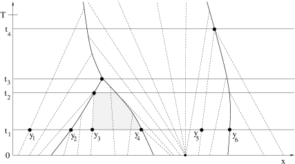
Figure 2: Proving that, under condition (C1), the solution $v$ of (5.1) is a regulated function. Here we choose the curves $\gamma_{j}$ to be the generalized characteristics through the points $y_{1},\ldots,y_{6}$. Notice that the values of the solution over the entire shaded region coincide with the values taken at time $t_{1}$ on the interval $\,]y_{3},y_{4}[\,$.

Proof.

1. Assume first that the condition (C1) holds. To fix the ideas, assume that $v_{0}(x)\in[-R,R]$ for all $x\in{\mathbb{R}}$, and Moreover, let $\varepsilon>0$ and an interval $[x_{1},x_{2}]$ be given. By the strict convexity of the flux, at any time $t>0$ the solution $v(t,\cdot)$ satisfies Oleinik’s inequality

$$v(t,y)-v(t,x)~{}\leq~{}{y-x\over\lambda t}\,,\qquad\quad\hbox{for all}~{}x<y.$$ (5.2)

Choose $t_{1}=\varepsilon/2$. Since $v(t_{1},\cdot)$ has locally bounded variation, we can choose finitely many points

$$x_{1}-LT~{}=~{}y_{0}~{}<~{}y_{1}<~{}\cdots~{}<~{}y_{N}~{}<~{}y_{N+1}~{}=~{}x_{2}+LT$$ (5.3)

such that the total variation of $v(t_{1},\cdot)$ on each open interval $\,]y_{j},y_{j+1}[\,$ is $<\varepsilon$.

For $j=1,\ldots,N$, call $t\mapsto\gamma_{j}(t)$ the forward generalized characteristic starting at $y_{j}$. More precisely, $\gamma_{j}$ is the unique solution to the upper semicontinuous, convex valued differential inclusion

$$\dot{x}(t)~{}\in~{}\Big{[}g^{\prime}\bigl{(}v(t,x(t)+))\bigr{)},\,g^{\prime}\bigl{(}v(t,x(t)-))\bigr{)}\Big{]},\qquad x(t_{1})~{}=~{}y_{j}\,.$$ (5.4)

We observe that, since the flux function is strictly convex, at any given point $(t,x)$ the right and left limits of the entropy admissible solution $v$ satisfy

$$\lim_{y\to x+}v(t,y)~{}\leq~{}\lim_{y\to x-}v(t,y).$$

Oleinik’s inequality (5.2) guarantees the forward uniqueness of solutions to (5.4).

By forward uniqueness, there can be at most $N-1$ times where two or more of these characteristics meet. This happens when two shocks join together, or a genuine characteristic hits a shock. Let

$$t_{1}~{}<~{}t_{2}~{}<~{}~{}\cdots~{}~{}<~{}t_{m}~{}<~{}t_{m+1}~{}=~{}T$$

be a finite set of times containing all the interaction times, for some $m\leq N$. To satisfy the conditions (i)–(iii) in Definition 1 we proceed as follows. Consider the disjoint time intervals

$$[a_{i},b_{i}]~{}=~{}\left[t_{i},t_{i+1}-\varepsilon/(2N)\right].$$

Define the curves $\gamma_{i,k}$ to be the restrictions of $\gamma_{1},\ldots,\gamma_{N}$ to $[a_{i},b_{i}]$. Of course, if $\gamma_{j}$ and $\gamma_{\ell}$ coincide on $[a_{i},b_{i}]$, they are regarded as one single curve. Finally, we define the constant states as the right limits

$$\alpha_{i,k}~{}\doteq~{}v\bigl{(}a_{i},\gamma_{i,k}(a_{i})+\bigr{)}.$$ (5.5)

It is now easy to check that all conditions (i)–(iii) in Definition 1 are satisfied. Indeed, the set of values attained by the solution $v$ satisfies

$$\Big{\{}v(t,x)\,;~{}t\in[a_{i},b_{i}],\;\gamma_{i,k-1}(t)<x<\gamma_{i,k}(t)\Big{\}}\;\subseteq\;\Big{\{}v(a_{i},x)\,;~{}\gamma_{i,k-1}(a_{i})<x<\gamma_{i,k}(a_{i}))\Big{\}}.$$

Since the total variation of $v(a_{i},\cdot)$ on the open interval $\,\bigl{]}\gamma_{i,k-1}(a_{i}),~{}\gamma_{i,k}(a_{i}))\bigr{[}\,$ is $<\varepsilon$, this proves (1.5).

Next, we observe that the speed of a genuine characteristic is constant in time, while the speed of a shock is a function of bounded variation. In all cases $\dot{\gamma}_{j}(\cdot)$ has bounded variation, hence it is a regulated function, as required in (ii). Finally, our construction yields

$$T-\sum_{i}(b_{i}-a_{i})~{}=~{}T-\sum_{i=1}^{m}(t_{i+1}-\frac{\varepsilon}{2N}-t_{i})~{}\leq~{}t_{1}+\varepsilon/2~{}=~{}\varepsilon,$$

proving (iii).

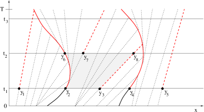
Figure 3: If the flux function has an inflection point, characteristics can originate from a shock, with tangential speed. In this case, the values attained by the solution $v(t,x)$ over the shaded region (bounded by the points $y_{2},y_{3},y_{8},y_{6}$) are not contained in the set of values attained at time $t_{1}$ over the open interval $]y_{2},y_{3}[\,$. For this reason, at some time $t_{2}$ sufficiently close to $t_{1}$ we need to insert an additional interface, along the characteristic starting at $y_{7}$.

2. Next, we consider the case where (C2) holds. The main difference is that now forward characteristics may not be unique. Indeed, as shown in Fig 3, characteristics can emerge to the right of a shock, with tangential velocity. To cope with this issue, the previous construction can be modified as follows.

Given $\varepsilon>0$, choose $t_{1}=\varepsilon/2$. At time $t_{1}$, choose points $y_{j}$ as in (5.3) so that the total variation of $v(t_{1},\cdot)$ on each open interval $\,]y_{j},y_{j+1}[\,$ is $<\varepsilon/4$. For $j=1,\ldots,N$, call $t\mapsto\gamma_{j}(t)$ the minimal forward generalized characteristic starting at $y_{j}$. More precisely,

$$\gamma_{j}(t)~{}\doteq~{}\inf~{}\bigl{\{}x(t)\,;~{}~{}x(\cdot)~{}\hbox{is a solution of}~{}\eqref{DI}\big{\}}.$$

Call $t_{2}^{\prime}>t_{1}$ the first time where two or more of the curves $\gamma_{j}$ join together. We remark that in this case it is no longer true that

$$\Big{\{}v(t,x)\,;~{}~{}t\in[t_{1},t^{\prime}_{1}],~{}~{}\gamma_{j-1}(t)<x<\gamma_{j}(t)\Big{\}}~{}\subseteq~{}\Big{\{}v(t_{1},x)\,;~{}~{}\gamma_{j-1}(t_{1})<x<\gamma_{j}(t_{1}))\Big{\}},$$

because of the characteristics emerging to the right of a shock. However, by the regularity estimates in [20, 24], there exists a constant $K$ such that, for all $t\geq t_{1}$ and $x\in{\mathbb{R}}$,

$$v(t,x)~{}>~{}\bar{s}+{\varepsilon\over 4}\qquad \Longrightarrow \qquad v_{x}(t,x)~{}<~{}K,$$

$$v(t,x)~{}<~{}\bar{s}-{\varepsilon\over 4}\qquad \Longrightarrow \qquad v_{x}(t,x)~{}>\,-K,$$

with $\bar{s}$ as in (C2). As a consequence, we can find $\delta_{0}>0$ such that, on any interval of the form $[\tau,\tau+\delta]$ with $\tau\geq t_{1}$, the total strength of all rarefaction waves emerging tangentially from a shock is $\leq 3\varepsilon/4$. Choosing $t_{2}\doteq\min\{t_{1}^{\prime},t_{1}+\delta\}$, the total oscillation of $v$ over each domain

$$\bigl{\{}(t,x)\,;~{}~{}t\in[t_{1},t_{2}],~{}~{}\gamma_{j-1}(t)<x<\gamma_{j}(t)\bigr{\}}$$

is $\leq\varepsilon$. At time $t_{2}$ we can insert some additional points $y_{k}$, so that the total oscillation of $v(t_{2},\cdot)$ on each open interval bounded by the points $\gamma_{j}(t_{2})$ and $y_{k}$ is $\leq\varepsilon/4$, and repeat the construction up to a time $t_{3}>t_{2}$, etc.

To prove that the total number of these time intervals remains finite, we observe that the total strength of all rarefaction waves emerging tangentially from a shock is finite. Indeed, these waves can be generated only when a rarefaction hits a shock form the left. This produces a decrease in the total variation. We thus have an estimate of the form

$$\begin{array}[]{c}[\hbox{total amount of rarefaction waves emerging tangentially from a shock,}\\[2.84526pt] \qquad\qquad\qquad\hbox{in the region where $|v-\bar{s}|>\varepsilon/4$}]~{}\leq~{}C\cdot\hbox{Tot.Var.}\{\bar{v}\},\end{array}$$

for some constant $C$. This ensures that the total number of additional points $y_{k}$ which we need to add during the inductive procedure is a priori bounded. Defining the constant states $\alpha_{ik}$ as in (5.5), the remainder of the proof is achieved in the same way as in case (C1). MM     

Remark. As shown in Fig. 4, the conclusion of Theorem 5.1 may fail if $g$ has two inflection points. Indeed, in this case a solution $v$ can have a pair of large shocks splitting apart and joining together infinitely many times. Nothing prevents the awkward situation where the two shock curves $\gamma_{1}(t)\leq\gamma_{2}(t)$ coincide on a Cantor-like set of times, totally disconnected but with positive measure. In this case, the conditions introduced in Definition 1 cannot be satisfied. Of course, this does not preclude the uniqueness of vanishing viscosity solutions of the triangular system (1.8). It simply yields a problem outside the scope of the present results.

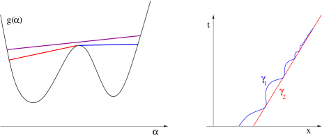
Figure 4: Left: a flux function $g$ with two inflection points. Right: for this flux, one can construct a solution having two large shocks splitting apart and joining together infinitely many times.

6 Concluding remarks

In this paper we established the existence and uniqueness of vanishing viscosity solutions for scalar conservation laws such as (1.1), where the flux function $f(t,x,\omega)=F\left(v(t,x),\omega\right)$ is discontinuous in both $t$ and $x$. See [8] for results of well posedness for fluxes with BV regularity with respect to the variable $t$.

In turn, the result yields the existence and uniqueness of solutions for the triangular system (1.8), under suitable assumptions on $g$. The system (1.8) may lose hyperbolicity where the two eigenvalues as well as the two eigenvectors coincide. We remark that it is well-known that the total variation for $u$ can blow up in finite time due to nonlinear resonances.

Our result applies beyond the case where $v(t,x)$ is a solution of a scalar conservation law. In particular, a regulated function $v(t,x)$ can have discontinuities also along lines where $t$ is constant. An application is provided by polymer flooding in two phase flow, with adsorption in rough porous media. This leads to a system of equations having the form

$$s_{t}+f(s,c,\kappa)_{x} = 0,$$

$$(m(c)+cs)_{t}+(c\,f(s,c,\kappa))_{x} = 0,$$

$$\kappa_{t} = 0.$$

The model describes an immiscible flow of water and oil phases, where polymers are dissolved in the water phase. Here $s$ is the saturation of the water phase, $c$ is the fraction of polymer in the water phase, and $\kappa=\kappa(x)$ denotes the varying porous media. In the case of rough media, $\kappa(x)$ can be discontinuous. The function $f$ is the fractional flow for the water phase, where the map $s\to f$ is typically S-shaped. The function $m(c)$ denotes the adsorption of polymers into the porous media, satisfying $m^{\prime}>0,m^{\prime\prime}<0$.

A global Riemann solver for this $3\times 3$ system was constructed in [38]. The results in the present paper suggest a possible way to solve general Cauchy problem. The connection is best revealed using a Lagrangian coordinate system $(\phi,\psi)$, defined as

$$\phi_{x}=-s,\qquad\phi_{t}=f(s,c,\kappa),\qquad\phi(0,0)=0,\qquad\psi=x.$$

In these coordinates, the equations take the form

$$\left(\frac{s}{f(s,c,\kappa)}\right)_{\phi}-\left(\frac{1}{f(s,c,\kappa)}\right)_{\psi} = 0,$$

$$m(c)_{\phi}+c_{\psi} = 0,$$

$$\kappa_{\phi} = 0.$$

We observe that the equations for $\kappa$ and $c$ are both decoupled, and can be solved separately. Treating $\phi$ as a time and $\psi$ as a space variable, the solution $c(\phi,\psi)$ is a regulated function, while the jumps in $\kappa$ occur along lines parallel to the $\phi$ axis. The system can thus be reduced to the first equation. This is a scalar conservation law where the flux depends on time and space in a regulated way. Details will be given in a future work.

Acknowledgment. The research of the first author was partially supported by NSF, with grant DMS-1411786: Hyperbolic Conservation Laws and Applications. The research of the second author was partially supported by the PRIN 2015 project Hyperbolic Systems of Conservation Laws and Fluid Dynamics: Analysis and Applications. The second author acknowledges the hospitality of the Department of Mathematics, Penn State University - May 2017.

References

• [1] J. Adimurthi and V. Gowda, Conservation laws with discontinuous flux. J. Math. Kyoto University 43 (2003), 27–70.
• [2] J. Adimurthi and V. Gowda, Godunov-type methods for conservation laws with a flux function discontinuous in space. SIAM J. Numer. Anal. 42 (2004), 179–208.
• [3] B. Andreianov, K. H. Karlsen, and N. H. Risebro, On vanishing viscosity approximation of conservation laws with discontinuous flux. Netw. Heterog. Media 5 (2010), 617–633.
• [4] B. Andreianov, K. H. Karlsen, and N. H. Risebro, A theory of $L^{1}$-dissipative solvers for scalar conservation laws with discontinuous flux. Arch. Ration. Mech. Anal. 201 (2011), 27–86.
• [5] E. Audusse and B. Perthame, Uniqueness for scalar conservation laws with discontinuous flux via adapted entropies. Proc. Roy. Soc. Edinburgh Sect. A 135 (2005), 253–265.
• [6] F. Bachmann and J. Vovelle, Existence and uniqueness of entropy solution of scalar conservation laws with a flux function involving discontinuous coefficients, Comm. Partial Diff. Equat. 31 (2006), 371–395.
• [7] A. Bressan, Hyperbolic systems of conservation laws. The one dimensional Cauchy problem, Oxford University Press, 2000.
• [8] G. M. Coclite and N. H. Risebro, Conservation laws with time dependent discontinuous coefficients. SIAM J. Math. Anal. 36 (2005), 1293–1309.
• [9] G. M. Coclite and N. H. Risebro, Viscosity solutions of Hamilton-Jacobi equations with discontinuous coefficients. J. Hyperbolic Differ. Equ. 4 (2007), 771–795.
• [10] M. G. Crandall, The semigroup approach to first order quasilinear equations in several space variables. Israel J. Math. 12 (1972), 108–132.
• [11] M. G. Crandall and T. M. Liggett, Generation of semigroups of nonlinear transformations on general Banach spaces. Amer. J. Math. 93 (1971), 265–298.
• [12] G. Crasta, V. De Cicco, and G. De Philippis, Kinetic formulation and uniqueness for scalar conservation laws with discontinuous flux. Comm. Partial Differential Equations 40 (2015), 694–726.
• [13] G. Crasta, V. De Cicco, G. De Philippis, and F. Ghiraldin, Structure of solutions of multidimensional conservation laws with discontinuous flux and applications to uniqueness. Arch. Ration. Mech. Anal. 221 (2016), 961–985.
• [14] C. Dafermos, Hyperbolic Conservation Laws in Continuum Physics. Third edition. Springer-Verlag, Berlin, 2010.
• [15] S. Diehl. Scalar conservation laws with discontinuous flux function. I. The viscous profile condition. Comm. Math. Phys. 176 (1996), 23–44.
• [16] D. H. Fremlin, Measure theory. Vol. 2, Torres Fremlin, Colchester, 2003.
• [17] M. Garavello, R. Natalini, B. Piccoli, and A. Terracina, Conservation laws with discontinuous flux. Netw. Heter. Media 2 (2007), 159–179.
• [18] T. Gimse and N. H. Risebro, Riemann problems with a discontinuous flux function. In Proc. Third Internat. Conf. on Hyperbolic Problems. Theory, Numerical Method and Applications. (B. Engquist, B. Gustafsson. eds.) Studentlitteratur/Chartwell-Bratt, Lund-Bromley, (1991), pp. 488-502.
• [19] T. Gimse and N. H. Risebro, Solution of the Cauchy problem for a conservation law with discontinuous flux function. SIAM J. Math. Anal. 23 (1992), pp. 635–648.
• [20] O. Glass, An extension of Oleinik’s inequality for general 1D scalar conservation laws. J. Hyperbolic Differ. Eq. 5 (2008), 113–165.
• [21] G. Guerra and W. Shen, Backward Euler Approximations for Conservation Laws with Discontinuous Flux. Preprint (2018).
• [22] D. Henry. Geometric Theory of Semilinear Parabolic Equations. Lecture Notes in Math. 840, Springer-Verlag, Berlin, 1981.
• [23] E. L. Isaacson and J. B. Temple, Analysis of a singular hyperbolic system of conservation laws, J. Differential Equations 65 (1986), 250–268.
• [24] H. K. Jenssen and C. Sinestrari, On the spreading of characteristics for non-convex conservation laws, Proc. Royal Soc. Edinburgh Sect. A 131 (2001), 909–925.
• [25] K. H. Karlsen, M. Rascle and E. Tadmor, On the existence and compactness of a two-dimensional resonant system of conservation laws, Commun. Math. Sci. 5, (2007), 253–265.
• [26] R. A. Klausen and N. H. Risebro, Stability of conservation laws with discontinuous coefficients. J. Differential Equations 157, (1999), 41–60.
• [27] C. Klingenberg and N. H. Risebro, Convex conservation laws with discontinuous coefficients, existence, uniqueness and asymptotic behavior. Comm. Partial Diff. Equat. 20 (1995), 1959–1990.
• [28] C. Klingenberg and N. H. Risebro, Stability of a resonant system of conservation laws modeling polymer flow with gravitation. J. Differential Equations 170, (2001), 344–380.
• [29] S. Kruzhkov, First-order quasilinear equations with several space variables, Mat. Sb. 123 (1970), 228–255. English transl. in Math. USSR Sb. 10 (1970), 217–273.
• [30] A. Lunardi, Analytic Semigroups and Optimal Regularity in Parabolic Equations. Birkhauser, Basel, 1995.
• [31] R. H. Martin, Nonlinear operators and differential equations in Banach spaces. Wiley-Interscience, New York-London-Sydney, 1976.
• [32] D. Mitrovic, New entropy conditions for scalar conservation laws with discontinuous flux. Discr. Cont. Dyn. Syst. 30 (2011), 1191-1210.
• [33] H. L. Royden and P. M. Fitzpatrick Real analysis. Pearson Prentice Hall, Boston, 2010.
• [34] N. Seguin and J. Vovelle, Analysis and approximation of a scalar conservation law with a flux function with discontinuous coefficients. Math. Models Methods Appl. Sci. 13 (2003), 221–257.
• [35] G. Sell and Y. You, Dynamics of Evolutionary Equations. Springer-Verlag, New York, 2002.
• [36] D. Serre, Systems of Conservation Laws I, II, Cambridge University Press, 2000.
• [37] W. Shen, On the Cauchy problem for polymer flooding with gravitation, J. Differential Equations 261 (2016), 627–653.
• [38] W. Shen, Global Riemann Solvers for Several $3\times 3$ Systems of Conservation Laws with Degeneracies. Preprint, 2017.
• [39] A. Tveito, and R. Winther. Existence, uniqueness, and continuous dependence for a system of hyperbolic conservation laws modeling polymer flooding. SIAM J. Math. Anal. 22 (1991), 905–933.