Facial Landmark Point Localization using Coarse-to-Fine Deep Recurrent Neural Network

Abstract

The accurate localization of facial landmarks is at the core of face analysis tasks, such as face recognition and facial expression analysis, to name a few. In this work we propose a novel localization approach based on a Deep Learning architecture that utilizes dual cascaded CNN subnetworks of the same length, where each subnetwork in a cascade refines the accuracy of its predecessor. The first set of cascaded subnetworks estimates heatmaps that encode the landmarks’ locations, while the second set of cascaded subnetworks refines the heatmaps-based localization using regression, and also receives as input the output of the corresponding heatmap estimation subnetwork. The proposed scheme is experimentally shown to compare favorably with contemporary state-of-the-art schemes.

1 Introduction

The localization of facial landmark points, such as eyebrows, eyes, nose, mouth and jawline, is one of the core computational components in visual face analysis, and is applied in a gamut of applications: face recognition [1], face verification [2], and facial attribute inference [3], to name a few. Robust and accurate localization entails difficulties due to varying face poses, illumination, resolution variations, and partial occlusions, as depicted in Fig. 1.

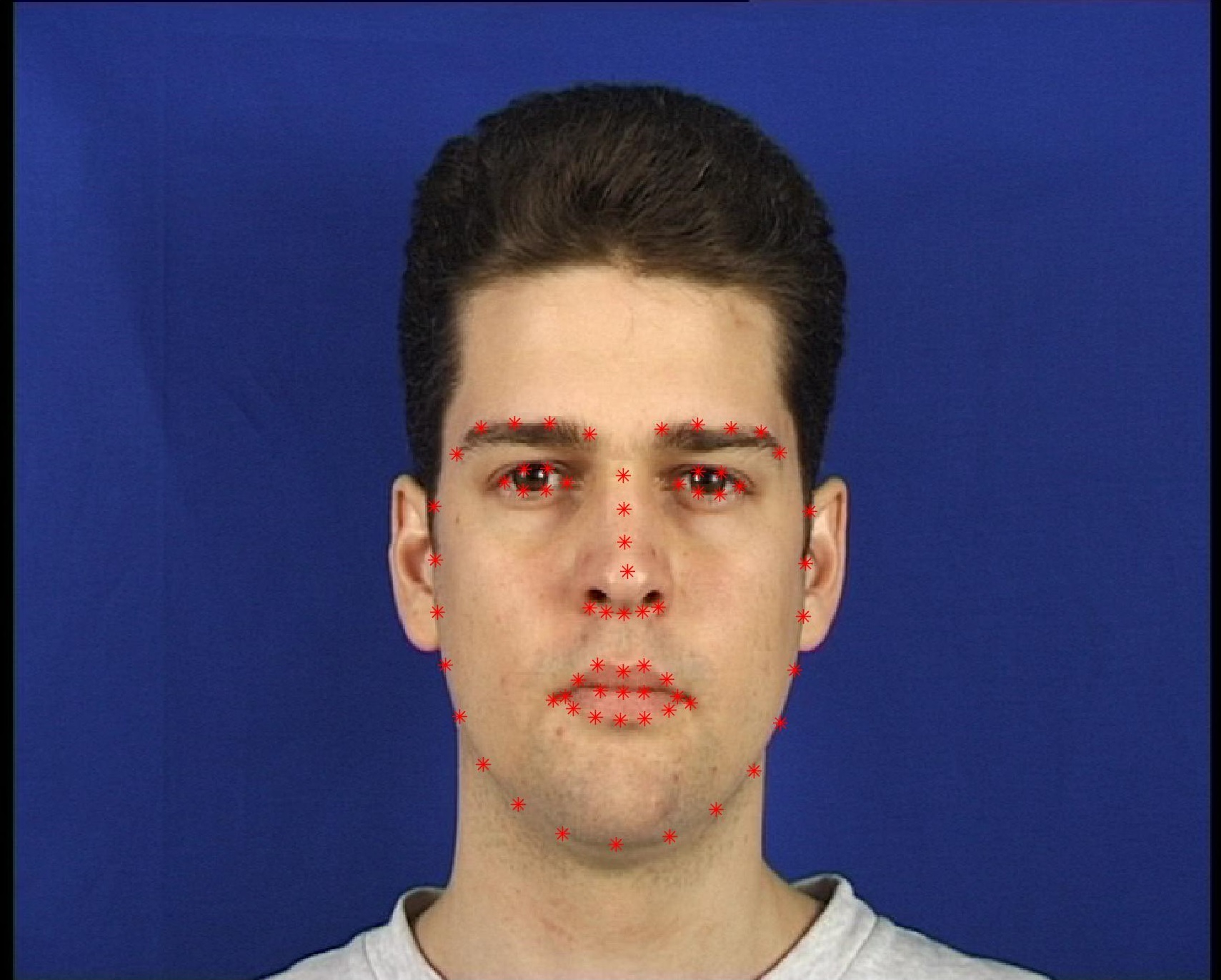
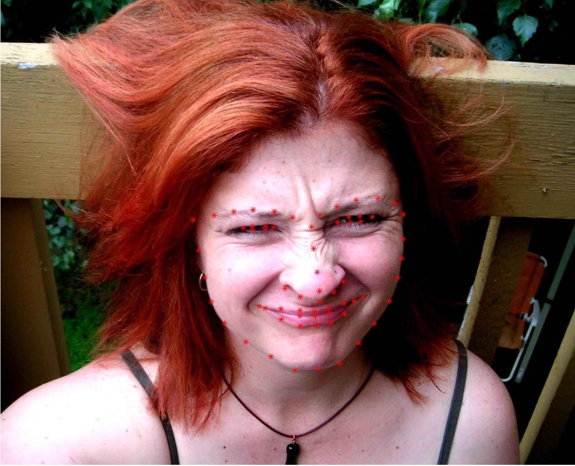
Figure 1: Facial landmark localization. Each image feature, marked by a point is considered a particular landmark and is localized individually. (a) A frontal face image from the XM2VTS datasets [4]. (b) An image from the Helen dataset [5] characterized by a non-frontal pose and expression variation, making the localization challenging.

Classical face localization schemes such as Active Appearance Models (AAM) [6] and Active shape models (ASM) [7] apply generative models aiming to learn a parametric statistical model of the face shape and its gray-level appearance in a training phase. The model is applied in test time to minimize the residual between the training image and the synthesized model. Parametric shape models such as Constrained Local Models (CLM) [8], utilize Bayesian formulations for shape constrained searches, to estimate the landmarks iteratively. Nonparametric global shape models [9] apply SVM classification to estimate the landmarks under significant appearance changes and large pose variations.

Regression based approaches [10, 11] learn high dimensional regression models that iteratively estimate landmarks positions using local image features, and showed improved accuracy when applied to in-the-wild face images. Such schemes are initiated using an initial estimate and are in general limited to yaw, pitch and head roll angles of less than $30{{}^{\circ}}$.

Following advances in object detection, parts-based models were applied to face localization [12, 13] where the facial landmarks and their geometric relationships are encoded by graphs. Computer vision was revolutionized by Deep Learning-based approaches that were also applied to face localization [14, 15, 16], yielding robust and accurate estimates. Convolutional neural networks (CNNs) extract high level features over the whole face region and are trained to predict all of the keypoints simultaneously, while avoiding local minima. In particular, heatmaps were used in CNN-based landmark localization schemes following the seminal work of Pfister et al. [17], extended by the iterative formulation by Belagiannis and Zisserman [18].

In this work we propose a novel Deep Learning-based framework for facial landmark localization that is formulated as a Cascaded CNN (CCNN) consisting of dual cascaded heatmaps and regression subnetworks. A outline of the architecture of the proposed CNN is depicted in Fig. 2, where after computing the feature maps of the entire image, each facial landmark is coarsely localized by a particular heatmap, and all localizations are refined by regression subnetworks. In that we extend prior works [17, 18] where iterative heatmaps computations were used, without the additional refinement subnetwork proposed in our work. The heatmaps are estimated using a Cascaded Heatmap subnetwork (CHCNN) consisting of multiple successive heatmap-based localization subnetworks, that compute a coarse-to-fine estimate of the landmark localization. This localization estimate is refined by applying the Cascaded Regression CNN (CRCNN) subnetwork. The cascaded layers in both the CHCNN and CRCNN are non-weight-sharing, allowing to separately learn a particular range of localizations. The CCNN is experimentally shown to compare favourably with contemporary state-of-the-art face localization schemes. Although this work exemplifies the use of the proposed approach in the localization of facial landmarks, it is of general applicability and can be used for any class of objects, given an appropriate annotated training set.

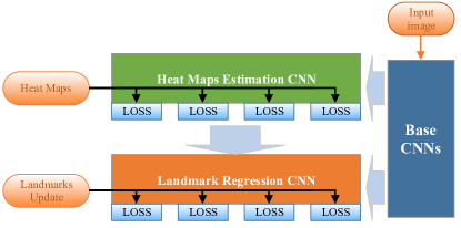
Figure 2: The outline of the proposed CCNN framework. The CCNN consists of Base CNNs that are proceeded by the Cascaded Heatmap subnetwork (CHCNN) that estimates the heatmaps and the Cascaded Regression CNN (CRCNN) that refines the heatmaps localization via pointwise regression.

Thus, we propose the following contributions:

First, we derive a face localizations scheme based on CNN-based heatmaps estimation and refinement by a corresponding regression CNN.

Second, both heatmap estimation and regression are formulated as cascaded subnetworks that allow iterative refinement of the localization accuracy. To the best of our knowledge, this is the first such formulation for the face localization problem.

Last, the proposed CCNN framework is experimentally shown to outperform contemporary state-of-the-art approaches.

This paper is organized as follows: Section 2 provides an overview of the state-of-the-art techniques for facial landmark localization, while Section 3 introduces the proposed CCNN and its CNN architecture. The experimental validation and comparison to state-of-the-art methods is detailed in Section 4. Conclusions are drawn in Section 5

2 Related work

The localization of facial landmarks, being a fundamental computer vision task, was studied in a multitude of works, dating back to the seminal results in Active Appearance Models (AAM) [6] and Constrained Local Models (CLM) [8] that paved the way for recent localization schemes. In particular, the proposed scheme relates to the Cascaded Shape Regression (CSR), [19] and Deep Learning-based [15, 14, 20, 21, 22] models.

CSR schemes localize the landmark points explicitly by iterative regression, where the regression estimates the localization refinement offset using the local image features computed at the estimated landmarks locations. Such schemes are commonly initiated by an initial estimate of the landmarks based on an average face template, and a bounding box of the face detected by a face detector, such as Viola-Jones [23]. Thus, the Supervised Descent Method by Xiong and De-la-Torre [11] learned a cascaded linear regression using SIFT features [24] computed at the estimated landmark locations. Other schemes strived for computational efficiency by utilizing Local Binary Features (LBF) that are learnt by binary trees in a training phase. Thus, Ren et al. in [25] proposed a face alignment technique achieving 3000 fps by learning highly discriminative LBFs for each facial landmark independently, and the learned LBFs are used to jointly learn a linear regression to estimate the facial landmarks’ locations.

Chen et al. [26] applied random regression forests to landmark localization using Haar-like local image features to achieve computational efficiency. Similarly, a discriminative regression approach was proposed by Asthana et al. [27] to learn regression functions from the image encodings to the space of shape parameters. A cascade of a mixture of regressors was suggested by Tuzel et al. [28], where each regressor learns a regression model adapted to a particular subspace of pose and expressions, such as a smiling face turned to the left. Affine invariance was achieved by aligning each face to a canonical shape before applying the regression.

A parts-based approach for a unified approach to face detection, pose estimation, and landmark localization was suggested by Zhu and Ramanan [12], where the facial features and their geometrical relations are encoded by the vertices of a corresponding graph. The inference is given by a mixture of trees trained using a training set. An iterative coarse-to-fine refinement implemented in space-shape was introduced by Zhu et al. [13], where the initial coarse solution allows to constrain the search space of the finer shapes. This allows to avoid suboptimal local minima and improves the estimation of large pose variations.

Deep Learning was also applied to face alignment by extending regression-based schemes for face alignment. The Mnemonic Descent Method by Trigeorgis et al. [19] combines regression as in CSR schemes, with feature learning using Convolutional Neural Networks (CNNs). The image features are learnt by the convolution layers, followed by a cascaded neural network that is jointly trained, yielding an end-to-end trainable scheme.

Autoencoders were applied by Zhang et al. [29] in a coarse-to-fine scheme, using successive stacked autoencoders. The first subnetwork predicts an initial estimate of the landmarks utilizing a low-resolution input image. The following subnetworks progressively refine the landmarks’ localization using the local features extracted around the current landmarks. A similar CNN-based approach was proposed by Shi et al. [30], where the subnetworks were based on CNNs, and a coarse face shape is initially estimated, while the following layers iteratively refine the face landmarks. CNNs were applied by Zhou et al. [31] to iteratively refine a subset of facial landmarks estimated by preceding network layers, where each layer predicts the position and rotation angles of each facial feature. Xiao et al. in [20] introduced a cascaded localization CNN using cascaded regressions that refine the localization progressively. The landmark locations are refined sequentially at each stage, allowing the more reliable landmark points to be refined earlier, where LSTMs are used to identify the reliable landmarks and refine their localization.

A conditional Generative Adversarial Network (GAN) was applied by Chen et al. [32] to face localization to induce geometric priors on the face landmarks, by introducing a discriminator that classifies real vs. erroneous (“fake”) localizations. A CNN with multiple losses was derived by Ranjan et al. in [14] for simultaneous face detection, landmarks localization, pose estimation and gender recognition. The proposed method utilizes the lower and intermediate layers of the CNN followed by multiple subnetworks, each with a different loss, corresponding to a particular tasks, such as face detection etc. Multi-task estimation of multiple facial attributes, such as gender, expression, and appearance attributes was also proposed by Zhang et al. [15], and was shown to improve the estimation robustness and accuracy.

Multi-task CNNs with auxiliary losses were applied by Sina et al. [33] for training a localization scheme using partially annotated datasets where accurate landmark locations are only provided for a small data subset, but where class labels for additional related cues are available. They propose a sequential multitasking scheme where the class labels are used via auxiliary losses. An unsupervised landmark localization scheme is also proposed, where the model is trained to produce equivalent landmark locations with respect to a set of transformations that are applied to the image.

Pfister et al. [17] introduced the use of heatmaps for landmark localization by CNN-based formulation. It was applied to human pose estimation in videos where the landmark points marks body parts, and optical flow was used to fuse heatmap predictions from neighboring frames. This approach was extended by Belagiannis and Zisserman by deriving a cascaded heatmap estimation subnetwork, consisting of multiple heatmap regression units, where the heatmap is estimated progressively such that each heatmap regression units received as input its predecessor’s output. This school of thought is of particular interest to our work that is also heatmaps-based, but also applies a cascaded regression subnetwork that refines the heatmap estimate.

Bulat and Tzimiropoulos [34] applied convolutional heatmap regression to 3D face alignment, by estimating the 2D coordinates of the facial landmarks using a set of 2D heatmaps, one per landmark, estimated using a CNN with an $L_{2}$ regression loss. Another CNN is applied to the estimated heatmaps and the input RGB image to estimate the $Z$ coordinate. A scheme consisting of two phases was proposed by Shao et al. [22] where the image features are first estimated by a heatmap, and then refined by a set of shape regression subnetworks each adapted and trained for a particular pose.

Kowalski et al. [16] proposed a multistage scheme for face alignment. It is based on a cascaded CNN where each stage refines the landmark positions estimated at the previous one. The inputs to each stage are a face image normalized to a canonical pose, the features computed by the previous stage, and a heatmap computed using the results of the previous phase. The heatmap is not estimated by the CNN, and in that, this scheme differs significantly from the proposed scheme, and other schemes that directly estimate the heatmaps as part of the CNN [17, 22, 34].

TABLE I: Overview of contemporary state-of-the-art facial landmark localization schemes.

Paper	Training Sets	Test Sets	Pts#
Ren [25]	LFPW[9],	i-bug[35]	68
	Helen[5],	Helen+LFPW[5, 9]
	AFW,300-W	i-bug+Helen+LFPW
Ranjan [14]	AFLW[36]	i-bug	68
		AFLW[36]	21
Zhu [13]	LFPW,	i-bug	68
	Helen,	Helen+LFPW
	AFW,	i-bug+Helen+LFPW
	300-W	LFPW[9]
		Helen[5]
Zhang [15]	MAFL[37],	i-bug	68
	AFLW,	Helen+LFPW
	COFW[38],	i-bug+Helen+LFPW
	Helen,300-W	Helen
Xiao [20]	LFPW,	i-bug	68
	Helen,	Helen+LFPW
	AFW,	i-bug+Helen+LFPW
	300-W	LFPW
		Helen
Lai [21]	LFPW,	i-bug	68
	Helen,	Helen+LFPW
	AFW,	i-bug+Helen+LFPW
	300-W	LFPW
		Helen
Shao [22]	CelebA[39],	i-bug	68
	300-W,	Helen+LFPW
	MENPO[40]	i-bug+Helen+LFPW
Sina [33]	Helen,	i-bug	68
	AFW,	Helen+LFPW
	LFPW	i-bug+Helen+LFPW
Chen [41]	Helen,	i-bug	68
	300-W,	Helen+LFPW
	MENPO	i-bug+Helen+LFPW
Kowalski [16]	LFPW,	i-bug	68
	Helen,	Helen+LFPW
	AFW,	i-bug+Helen+LFPW
	300-W	300-W private test set
	LFPW,	i-bug
	Helen,AFW,	Helen+LFPW
	300-W,	i-bug+Helen+LFPW
	MENPO	300-W private test set
He [42]	LFPW,	i-bug	68
	Helen,AFW
	300-W,
	MENPO
Chen [32]	LFPW,	300-W private test set	68
	Helen,AFW
	i-bug,

Last, we summarize the different face localization approaches in Table I, where we detail the training and test datasets, as these are the basis for forming the experimental validation in Section 4.

3 Face Localization using cascaded CNNs

The face localization problem is the localization of a set of landmarks points ${P}=\left\{\mathbf{p}_{i}\right\}_{1}^{N}$, such that $\mathbf{p}_{i}$=$[x_{i},y_{i}]^{T},$ in a face image $I\in\mathbb{R}^{w\times h\times 3}$. The number of estimated points $N$ relates to the annotation convention used, and in this work we used $N=68$ landmark points following most contemporary works. The general and detailed outlines of the proposed CCNN’s architecture are depicted in Figs. 2 and 3, respectively. It comprises of three subnetworks, where the first is a pseudo-siamese (non-weight-sharing) subnetwork consisting of two subnetworks $\left\{BaseCNN_{1},BaseCNN_{2}\right\}$ that compute the corresponding feature maps $\left\{\mathbf{F}_{1},\mathbf{F}_{2}\right\}$ of the input image and an initial estimate of the heatmaps.

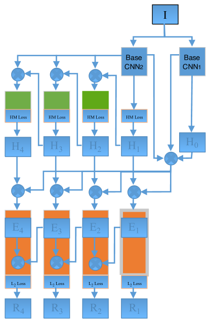
Figure 3: A schematic visualization of the proposed CCNN localization network. The input image is analyzed by the two Base subnetworks $\left\{BaseCNN_{1},BaseCNN_{2}\right\}$, and the Cascaded Heatmap CNN (CHCNN) consisting of four heatmap (HM) estimation units $H_{1}-H_{4}$. Their results are refined by the Cascaded Regression CNN (CHCNN) consisting of four regression units $R_{1}-R_{4}$. The symbol $\oplus$ relates to the concatenation of variables along their third dimension.

The second subnetwork is the cascaded heatmap subnetwork (CHCNN) that robustly estimates the heatmaps, that encode the landmarks, a single 2D heatmap per facial feature location. The heatmaps are depicted in Fig. 4. The CHCNN consists of $K=4$ cascaded 3D heatmaps estimation units, detailed in Section 3.2, that estimate $K$ 3D heatmaps $\{\mathbf{H}_{k}\}_{1}^{K}$ such that $\mathbf{H}_{k}\in\mathbb{R}^{64\times 64\times N}$. The cascaded formulation implies that each CHCNN subunit $\mathbf{H}_{k}$ is given as input the heatmap estimated by its preceding subunit $\mathbf{H}_{k-1}$, alongside the feature map $\mathbf{F}_{1}$. The heatmap subunits are non-weight-sharing, as each subunit refines a different estimate of the heatmaps. In that, the proposed schemes differs from the heatmaps-based pose estimation of Belagiannis and Zisserman [18] that applies weight-sharing cascaded units. The output of the CHCNN are the locations of the maxima of $\{\mathbf{H}_{k}\}_{1}^{K}$ denoted $\{\widehat{\mathbf{P}}_{k}\}_{1}^{K}$, such that $\widehat{\mathbf{P}}_{k}=\left\{\widehat{\mathbf{p}}_{k}^{i}\right\}$.

As the heatmap-based estimates $\{\widehat{\mathbf{P}}_{k}\}_{1}^{K}$ are given on a coarse grid, their locations are refined by applying the Cascaded Regression CNN (CRCNN) detailed in Section 3.2. The CRCNN consists of $K$ cascaded regression subunits $\{\mathbf{E}_{k}\}_{1}^{K}$, where each regression subunit $\mathbf{E}_{k}$ applies a regression loss to refine the corresponding heatmaps-based landmark estimate $\widehat{\mathbf{P}}_{k}$, and estimate the refinement $\Delta\widehat{\mathbf{P}}_{k}$

$$\Delta\widehat{\mathbf{P}}_{k}=vec\left(P_{k}\right)-vec\left(\widehat{\mathbf{P}}_{k}\right),$$ (1)

where $vec\left(\cdot\right)$ is a vectorized replica of the $N$ points in a set, and Eq. 1 is optimized using an $L_{2}$ loss.

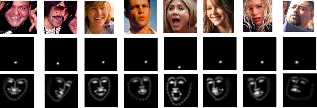
Figure 4: Visualizations of facial landmarks localization heatmaps. The first row shows the face images, while the second row depicts a corresponding single heatmap of a particular facial feature. The third row shows the corresponding $N=68$ points of all heatmap.

3.1 Base subnetwork

The Base subnetwork consists of two pseudo-siamese (non-weight-sharing) subnetworks detailed in Table II. The first part of the subnetwork, layers A1-A7 in Table II, computes the feature maps of the input image. The succeeding layers A8-A12 compute an estimate of the $N=68$ heatmaps, one per facial feature. These layers apply filters with wide $9\times 9$ support to encode the relations between neighboring facial features.

The base CNNs $\left\{BaseCNN_{1},BaseCNN_{2}\right\}$ and corresponding feature maps $\left\{\mathbf{F}_{1},\mathbf{F}_{2}\right\}$ are trained using different losses and backpropagation paths as depicted in Fig. 3. $BaseCNN_{1}$ is connected to the CRCNN and is thus adapted to the regression task, while $BaseCNN_{2}$ is connected to the CHCNN and its feature map $\mathbf{F}_{2}$ is adapted to the heatmaps estimation task. $BaseCNN_{2}$ computes the initial estimate of the heatmaps and is trained using a $L_{2}$ loss, while $BaseCNN_{1}$ is trained using the backpropagation of the CRCNN subnetwork.

TABLE II: Base subnetwork architecture. Given the input image, the base subnetwork estimates the feature map $F$ and the heatmap $H$. Two such non-weight-sharing subnetworks are used as depicted in Fig. 3.

$\mathbf{Layer}$	Feature Map	$\mathbf{F_{Size}}$	Stride	Pad
Input : $I$	256 x 256 x 3	-	-	-
A1-Conv	256 x 256 x 3	3 x 3	1 x 1	2 x 2
A1-ReLu	256 x 256 x 64	-	-	-
A2-Conv	256 x 256 x 64	3 x 3	1 x 1	2 x 2
A2-ReLu	256 x 256 x 64	-	-	-
A2-Pool	256 x 256 x 64	2 x 2	2 x 2	0 x 0
A3-Conv	128 x 128 x 64	3 x 3	1 x 1	2 x 2
A3-ReLu	128 x 128 x 64	-	-	-
A4-Conv	128 x 128 x 64	3 x 3	1 x 1	2 x 2
A4-ReLu	128 x 128 x 128	-	-	-
A4-Pool	128 x 128 x 128	2 x 2	2 x 2	0 x 0
A5-Conv	64 x 64 x 128	3 x 3	1 x 1	2 x 2
A5-ReLu	64 x 64 x 128	-	-	-
A6-Conv	64 x 64 x 128	3 x 3	1 x 1	2 x 2
A6-ReLu	64 x 64 x 128	-	-	-
A7-Conv	64 x 64 x 128	1 x 1	1 x 1	-
Output : $F$	64 x 64 x 128	-	-	-
A8-Conv	64 x 64 x 128	9 x 9	1 x 1	8 x 8
A8-ReLu	64 x 64 x 128	-	-	-
A9-Conv	64 x 64 x 128	9 x 9	1 x 1	8 x 8
A9-ReLu	64 x 64 x 128	-	-	-
A10-Conv	64 x 64 x 128	1 x 1	1 x 1	0 x 0
A10-ReLu	64 x 64 x 256	-	-	-
A11-Conv	64 x 64 x 256	1 x 1	1 x 1	0 x 0
A11-ReLu	64 x 64 x 256	-	-	-
A11-Dropout0.5	64 x 64 x 256	-	-	-
A12-Conv	64 x 64 x 256	1 x 1	1 x 1	0 x 0
A12-ReLu	64 x 64 x 68	-	-	-
Output : $H$	64 x 64 x 68	-	-	-

3.2 Cascaded heatmap estimation CNN

The heatmap images encode the positions of the set of landmarks points ${P}=\left\{\mathbf{p}_{i}\right\}_{1}^{N}$, by relating a single heatmap $\mathbf{H}^{i}$ per landmark $\mathbf{p}_{i}$ to the location of the maximum of $\mathbf{H}^{i}$, where the heatmaps are compute in a coarse resolution of $1/4$ of the input image resolution. The heatmaps are computed using the CHCNN subnetwork consisting of $K=4$ Heatmap Estimation Subunits (HMSU) detailed in Table III.

The cascaded architecture of the CHCNN implies that each heatmap subunit estimates a heatmap $\mathbf{H}_{k}$ and receives as input the heatmap $\mathbf{H}_{k-1}$ estimated by the previous subunit, and a feature map $\mathbf{F}_{2}$ estimated by the Base subnetwork $BaseCNN_{2}$. The different inputs are concatenated as channels such that the input is given by $\mathbf{F}_{2}\oplus\mathbf{H}_{k-1}$.

The HMSU architecture comprises of wide filters, $[7\times 7]$ and $[13\times 13]$ corresponding to layers B1 and B2, respectively, in Table III. These layers encode the geometric relationships between relatively distant landmarks. Each heatmap is trained with respect to a $L_{2}$ loss, and in the training phase, the locations of the facial landmarks are labeled by narrow Gaussians centered at the landmark location, to improve the training convergence.

TABLE III: The heatmap estimation subunit. The heatmap CNN (CHCNN) is a cascaded CNN consisting of a series of $K=4$ subunits. The input to each subunit is the output of the previous subunit and the feature map $F_{2}$.

$\mathbf{L_{Type}}$	Feature Map	$\mathbf{F_{Size}}$	Stride	Pad
Input : $F_{1}\oplus{H_{k-1}}$	64 x 64 x 136	-	-	-
B1-Conv	64 x 64 x 136	7 x 7	1 x 1	6 x 6
B1-ReLu	64 x 64 x 64	-	-	-
B2-Conv	64 x 64 x 64	13 x 13	1 x 1	12 x 12
B2-ReLu	64 x 64 x 64	-	-	-
B3-Conv	64 x 64 x 64	1 x 1	1 x 1	0 x 0
B3-ReLu	64 x 64 x 128	-	-	-
B4-Conv	64 x 64 x 128	1 x 1	1 x 1	0 x 0
B4-ReLu	64 x 64 x 68	-	-	-
Output : ${H_{k}}$	64 x 64 x 68	-	-	-
${L_{2}}$ regression loss

3.3 Cascaded regression CNN

The Cascaded regression CNN (CRCNN) is applied to refine the robust, but coarse landmark estimate computed by the CHCNN subnetwork. Similar to the CHCNN subnetwork detailed in Section 3.2, the CRCNN comprises of $K=4$ subunits $\left\{\mathbf{E}_{k}\right\}_{1}^{K}$ detailed in Table IV. Each subunit $\mathbf{E}_{k}$ is made of two succeeding subnetworks: the first computes a feature map of the regression CNN using layers C1-C3 in Table IV, while the second subnetwork, layers C4-C6 in Table IV, estimates the residual localization error. The input $x$ to each regression subunit $\mathbf{E}_{k}$ is given by

$$x=F_{1}\oplus F_{2}\oplus H_{k}\oplus H_{E},$$ (2)

that is a concatenation of both feature maps $F_{1}$ and $F_{2}$ computed by the Base CNNs, the corresponding heatmap estimate $H_{k}$ and a baseline heatmap estimate $H_{0}$. The output of the regression subunit $\mathbf{E}_{k}$ is the refinement term $\Delta\widehat{\mathbf{P}}_{k}$ as in Eq. 1, that is the refinement of the heatmap-based localization. It is trained using a $L_{2}$ regression loss, and the final localization output is given by the output of the last unit $\mathbf{E}_{K}$.

TABLE IV: The landmark regression subunit. The Cascaded regression CNN (CRCNN) is a cascaded CNN consisting of a series of $K=4$ subunits. The input to each subunit is the output of the previous regression subunit, the corresponding heatmap unit, as well as the feature maps $F_{1}$ and $F_{2}$.

$\mathbf{L_{Type}}$	Feature Map	$\mathbf{F_{Size}}$	Stride	Pad
Input :
$F_{1}\oplus F_{2}\oplus H_{k}\oplus H_{E}$	64 x 64 x 332	-	-	-
C1-Conv	64 x 64 x 332	7 x 7	2 x 2	5 x 5
C1-Pool	32 x 32 x 64	2 x 2	1 x 1	1 x 1
C2-Conv	32 x 32 x 64	5 x 5	2 x 2	3 x 3
C2-Pool	16 x 16 x 128	2 x 2	1 x 1	1 x 1
C3-Conv	16 x 16 x 128	3 x 3	2 x 2	1 x 1
C3-Pool	8 x 8 x 256	2 x 2	1 x 1	1 x 1
Output : $E_{k}$	8 x 8 x 256	-	-	-
Input : $E_{k}\oplus E_{k-1}$	8 x 8 x 512	-	-	-
C4-Conv	8 x 8 x 512	3 x 3	2 x 2	1 x 1
C4-Pool	4 x 4 x 512	2 x 2	1 x 1	1 x 1
C5-Conv	4 x 4 x 512	3 x 3	2 x 2	1 x 1
C5-Pool	2 x 2 x 1024	2 x 2	1 x 1	1 x 1
C6-Conv	2 x 2 x 1024	1 x 1	1 x 1	0 x 0
Output : $\Delta\widehat{P}_{k}$	1 x 1 x 136	-	-	-
$L_{2}$ regression loss

3.4 Discussion

The heatmap-based representation of the facial landmarks is essentially a general-purpose metric-space representation of a set of points. The use of smoothing filters applied to such representation relates to applying kernels to characterize a data point based on the geometry of the points in its vicinity [43, 44], where the use of filters of varying support allows approximate diffusion-like analysis at different scales. Moreover, applying multiple convolution layers and nonlinear activation functions to the heatmaps allows to utilize convolution kernels that might differ significantly from classical pre-designed kernels, such as Diffusion Kernels [43], as the filters in CNN-based schemes are optimally learnt given an appropriate loss.

In the proposed scheme the heatmap is used as a state variable that is initiated by the Base subnetwork (Section 3.1) and iteratively refined by using two complementary losses: the heatmap-based (Section 3.2) that induces the graph structure of the detected landmarks, and the coordinates-based representation, refined by pointwise regression (Section 3.3).

Such approaches might pave the way for other localization problems such as sensor localization [45] where the initial estimate of the heatmap is given by a graph algorithm, rather than image domain convolutions, but the succeeding CNN architecture would be similar to the CHCNN and CRCNN subnetworks, and we reserve such extensions to future work.

4 Experimental Results

The proposed CCNN scheme was experimentally evaluated using multiple contemporary image datasets used in state-of-the-art schemes, that differ with respect to the appearance and acquisition conditions of the facial images. We used the LFPW [9], M2VTS [4], Helen [5], AFW [46], i-bug [35], COFW [38], 300-W [47] and the MENPO challenge dataset [40].

In order to adhere to the state-of-the-art 300-W competition guidelines [19, 28] $N=68$ landmarks were used in all of our experiments, where the input RGB images were resized to $256\times 256$ dimensions, and the pixel values were normalized to $[-0.5,0.5]$. The heatmaps were computed at a $64\times 64$ spatial resolution, where the landmark’s labeling was applied using a symmetric Gaussian, with $\sigma=1.3$. The convolution layers of the CCNN were implemented with a succeeding batch normalization layer, and the training images were augmented by color changes, small angles rotation, scaling, and translations. The learning rate was changed manually and gradually, starting with $10^{-5}$ for the initial $30$ epochs, followed by $5\cdot 10^{-6}$ for the next five epochs, and was then fixed at $10^{-6}$ for the remainder of the training, where the CCNN was trained for 2500 epochs.

The localization accuracy per single face image was quantified by the Normalized Localization Error (NLE) between the localized and ground-truth landmarks

$$NLE=\frac{1}{N\cdot d}\sum\limits_{i=1}^{N}\left\|\widehat{\mathbf{p}}_{i}-\mathbf{p}_{i}\right\|_{2}$$ (3)

where $\widehat{\mathbf{p}}_{i}$ and $\mathbf{p}_{i}$ are the estimated and ground-truth coordinates, of a particular facial landmark, respectively. The normalization factor $d$ is either the inter-ocular distance (the distance between the outer corners of the eyes) [25, 40, 13], or the inter-pupil distance (the distance between the eye centers) [19].

The localization accuracy of a set of images was quantified by the average localization error and the failure rate, where we consider a normalized point-to-point localization error greater than 0.08 as a failure [19]. We also report the area under the cumulative error distribution curve (AUC_α) [19, 28], that is given by the area under the cumulative distribution summed up to a threshold $\alpha$. The proposed CCNN scheme was implemented in Matlab and the MatConvNet-1.0-beta23 deep learning framework [48] using a Titan X (Pascal) GPU.

Where possible, we quote the results reported in previous contemporary works, as most of them were derived using the 300-W competition datasets, where both the dataset and evaluation protocol are clearly defined. In general, we prefer such a comparative approach to implementing or training other schemes, as often, it is difficult to achieve the reported results, even when using the same code and training set.

4.1 300-W results

We evaluated the proposed CCNN approach using the 300-W competition dataset [35] that is a state-of-the-art face localization dataset of $3,837$ near frontal face images. It comprises of images taken from the LFPW, Helen, AFW, i-bug, and “300W private test set” datasets. Each image in these datasets was re-annotated in a consistent manner with $68$ landmarks and a bounding box per image was estimated by a face detector.

The CCNN was trained using the 300-W training set and the frontal face images of the Menpo dataset [40] that were annotated by 68 landmark points, same as in the 300-W dataset. The profile faces in the Menpo dataset were annotated by 39 landmark points that do not correspond to the 68 landmarks annotations, and thus could not be used in this work. The overall training set consisted of $11,007$ images.

The validation set was a subset of $2500$ images randomly drawn from the training set. The face images were extracted using the bounding boxes given in the 300-W challenge, where the shorter dimension was extended to achieve rectangular image dimensions, and the images were resized to a dimension of $256\times 256$ pixels.

4.1.1 300-W public testset

We compared the CCNN to contemporary state-of-the-art approaches using the Public and Private 300-W test-sets. The Public test-set was split into three test datasets following the split used in contemporary works [16, 49]. First, the Common subset consisting of the test-sets of the LFPW and Helen datasets (554 images overall). Second, the Challenging subset made of the i-bug dataset (135 images overall), and last, the 300-W public test-set (Full Set). The localization results of the other schemes in Tables V-VII are quoted as were reported by their respective authors.

The results are reported in Table V, and it follows that the proposed CCNN scheme compared favorably with all other scheme, outperforming other schemes in three out of the six test configurations. In particular, the proposed scheme outperforms all previous approaches when applied to the Challenging set that is the more difficult to localize.

TABLE V: Facial landmarks localization results of the 300-W Public dataset. We report the Normalized Localization Error (NLE) as a percentage using the 300-W public test set and its subsets. The best results are marked bold.

Method	Common set	Challenging set	Full Set
Inter-pupil normalization
LBF[25]	4.95	11.98	6.32
CFSS[13]	4.73	9.98	5.76
TCDCN[15]	4.80	8.60	5.54
RAR[20]	4.12	8.35	4.94
DRR[21]	4.07	8.29	4.90
Shao et al.[22]	4.45	8.03	5.15
Chen et al.[41]	3.73	7.12	4.47
DAN[16]	4.42	7.57	5.03
DAN-Menpo[16]	4.29	7.05	4.83
Robust FEC-CNN[42]	-	6.56	-
CCNN	4.55	5.67	4.85
Inter-ocular normalization
MDM[19]	-	-	4.05
k-Convuster[50]	3.34	6.56	3.97
DAN[16]	3.19	5.24	3.59
DAN-Menpo[16]	3.09	4.88	3.44
CCNN	3.23	3.99	3.44

We also depict in Fig. 5 the AUC_0.08 accuracy measure of the CCNN when applied to the Helen and LFPW testsets.

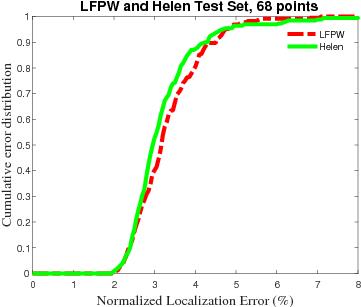
Figure 5: Facial localization results evaluated using the Helen and LFPW testsets. We report the Cumulative Error Distribution (CED) vs. the normalized localization error.

4.1.2 300-W private testset

We studied the localization of the 300W Private test set, LFPW and Helen datasets in Table VI where the proposed scheme prevailed in four out of the six test configurations.

TABLE VI: Localization results for the LFPW, Helen and 300-W Private Set. We report the Normalized Localization Error (NLE) as a percentage, where the best results are marked bold.

Method	LFPW	Helen	300-W Private Set
Inter-pupil normalization
CFSS[13]	4.87	4.63	-
TCDCN[15]	-	4.60	-
DRR[21]	4.49	4.02	-
CCNN	4.63	4.51	4.74
Inter-ocular normalization
RAR[20]	3.99	4.30	-
MDM[19]	-	-	5.05
DAN[16]	-	-	4.30
DAN-Menpo[16]	-	-	3.97
GAN[32]	-	-	3.96
CCNN	3.30	3.20	3.33

The AUC_0.08 measure and the localization failure rate are studied in Table VII, where we compared against contemporary schemes using the 300-W public and private test sets. It follows that the proposed CCNN scheme outperforms all other schemes in all test setups.

TABLE VII: AUC and failure rate of the face alignment scheme applied to the 300-W Public and Private test sets.

Test Set	Method	AUC0.08	Failure (%)
Inter-ocular normalization
300-W Public	ESR[10]	43.12	10.45
	SDM[11]	42.94	10.89
	CFSS[13]	49.87	5.08
	MDM[19]	52.12	4.21
	DAN[16]	55.33	1.16
	DAN-Menpo[16]	57.07	0.58
	CCNN	57.88	0.58
300-W Private	ESR[10]	32.35	17.00
	CFSS[13]	39.81	12.30
	MDM[19]	45.32	6.80
	DAN[16]	47.00	2.67
	DAN-Menpo[16]	50.84	1.83
	GAN[32]	53.64	2.50
	CCNN	58.67	0.83

We also used the 300-W private testset and the corresponding split of 300 Indoor and 300 Outdoor images, respectively, as these results were reported by the prospective authors as part of the 300-W challenge results [35]. Figures 6-8 depict the AUC_0.08 accuracy measure vs. NLE, that was normalized using the inter-ocular normalization. We show the results for the split of indoor, outdoor and combined (indoor+outdoor) test images in Figs. 6, 7 and 8, respectively. The results of the schemes we compare against are quoted from the 300-W challenge results[35]. It follows that for all three test subsets, the proposed CCNN scheme outperforms the contemporary schemes significantly.

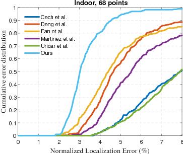
Figure 6: Facial localization results evaluated using the 300-W Indoor dataset. We report the Cumulative Error Distribution (CED) vs. the normalized localization error.

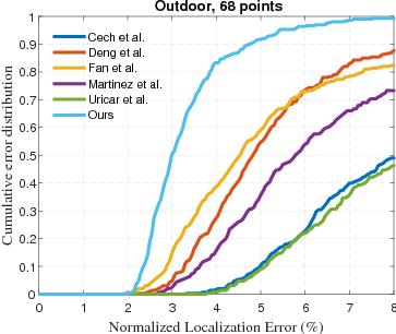
Figure 7: Facial localization results evaluated using the 300-W Outdoor dataset. We report the Cumulative Error Distribution (CED) vs. the normalized localization error.

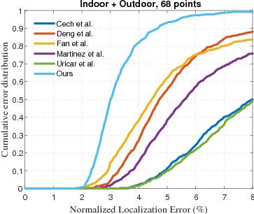
Figure 8: Facial localization results evaluated using the entire 300-W dataset. We report the Cumulative Error Distribution (CED) vs. the normalized localization error.

Figure 9 shows some of the estimated landmarks in images taken from the 300-W indoor and outdoor test sets. In particular, we show face images with significant yaw angles and facial expressions. These images exemplify the effectiveness of the proposed CCNN framework.

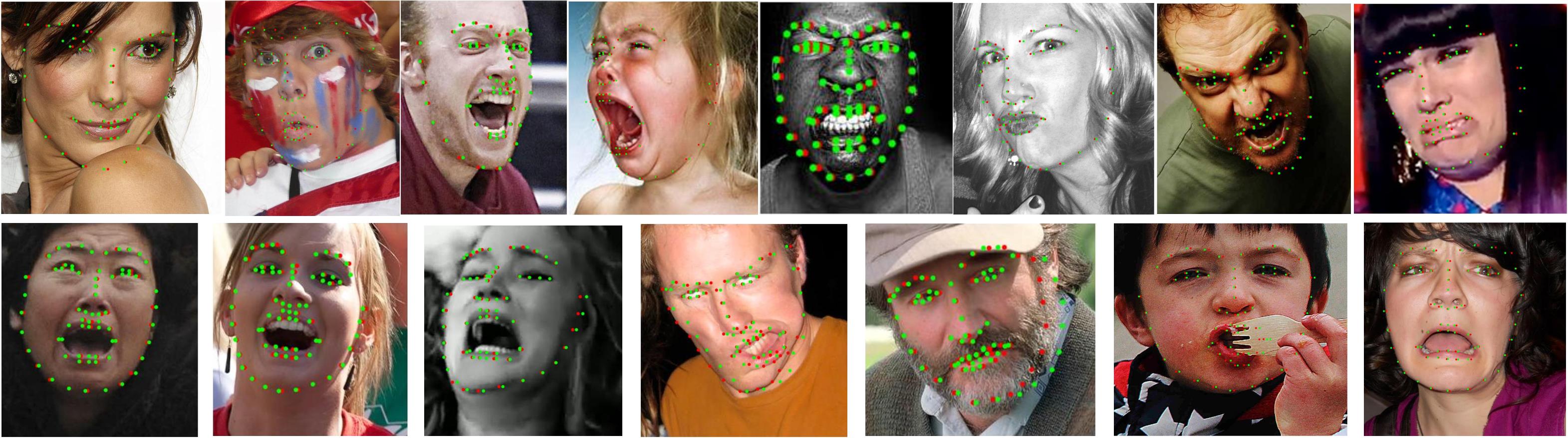
Figure 9: Facial landmarks localizations examples. The images are taken from the 300-W test set, where the red and green dots depict the groundtruth and estimated landmark points ,respectively, estimated by the proposed CCNN scheme.

4.2 COFW dataset results

The Caltech Occluded Faces in the Wild (COFW) dataset [38] is a challenging dataset consisting of $1,007$ faces depicting a wide range of occlusion patterns, and was annotated by Ghiasi and Fowlkes [51] with $68$ landmark points. The common train/test split is to use 500 images for training and the other 507 images for testing. Following previous works, we applied the same CCNN model as in Section 4.1 to the COFW testset (507 images) and compared the resulting accuracy with several state-of-the-art localization schemes. The experimental setup follows the work of Ghiasi and Fowlkes [51], where the results of prior schemes were also made public. In this setup the CFSS [13] and TCDCN [15] schemes were trained using the Helen68, LFPW68 and AFW68 datasets. The RCPR-occ scheme [38] was trained using the same training sets as the CCNN model, while the HPM and SAPM schemes,[51] were trained using Helen68 and LFPW68 datasets, respectively. The comparative results are depicted in Fig. 10 and it follows that the CCNN scheme outperforms the other contemporary schemes. For instance, for a localization accuracy of 0.05 the CCNN outperforms the CFSS, coming in second best, by close to 15%.

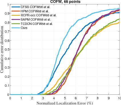
Figure 10: Facial localization results evaluated using the COFW dataset. We report the Cumulative Error Distribution (CED) vs. the normalized localization error.

4.3 Ablation study

We studied the effectivity of the proposed CCNN cascaded architecture by varying the number of cascades used in the CHCNN (heatmaps) and CRCNN (regression) subnetworks. For that we trained the CCNN using $K=\left\{1,2,3,4\right\}$ HCNN and CRCNN cascades with the same training sets and setup as in Section 4.1. The resulting CNNs were applied to the same test sets as in Sections 4.1 and 4.2. The results are depicted in Fig. 11, where we report the localization accuracy at the output of the CRCNN subnetwork. It follows that the more cascades are used the better the accuracy, and the most significant improvement is achieved for using more than a single cascade. Moreover, it seems that adding another cascade might improve the overall accuracy by $\sim 2\%$.

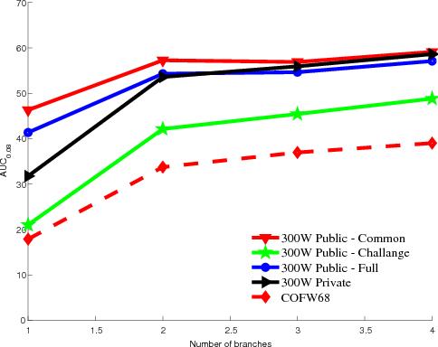
Figure 11: Ablation study results of the proposed CCNN scheme. We vary the number of cascades of both the CHCNN (heatmaps) and CRCNN (regression) subnetworks, and report the localization accuracy at the output of the CRCNN subnetwork.

5 Conclusions

In this work, we introduced a Deep Learning-based cascaded formulation of the coarse-to-fine localization of facial landmarks. The proposed cascaded CNN (CCNN) applied two dual cascaded subnetworks: the first (CHCNN) estimates a coarse but robust heatmap corresponding to the facial landmarks, while the second is a cascaded regression subnetwork (CRCNN) that refines the accuracy of CHCNN landmarks localization, via regression. The two cascaded subnetworks are aligned such that the output of each CHCNN unit is used as an input to the corresponding CRCNN unit, allowing the iterative refinement of the localization accuracy. The CCNN is an end-to-end solution to the localization problem that is fully data-driven and trainable, and extends previous results on heatmaps-based localization [52]. The proposed scheme is experimentally shown to be robust to large variations in head pose and its initialization. Moreover, it compares favorably with contemporary face localization schemes when evaluated using state-of-the-art face alignment datasets.

This work exemplifies the applicability of heatmaps-based landmarks localization. In particular, the proposed CCNN scheme does not utilize any particular appearance attribute of faces and can thus be applied, to the localization of other classes of objects of interest. In future, we aim to extend the proposed localization framework to the localization of sensor networks where the image domain CNN is reformulated as graph domain CNNs.

6 Acknowledgment

This work has been partially supported by COST Action 1206 “De-identification for privacy protection in multimedia content” and we gratefully acknowledge the support of NVIDIA^® Corporation for providing the Titan X Pascal GPU for this research work.

References

- [1] Z. Huang, X. Zhao, S. Shan, R. Wang, and X. Chen, “Coupling alignments with recognition for still-to-video face recognition,” in 2013 IEEE International Conference on Computer Vision, Dec 2013, pp. 3296–3303.
- [2] C. Lu and X. Tang, “Surpassing human-level face verification performance on lfw with gaussian face,” in Proceedings of the Twenty-Ninth AAAI Conference on Artificial Intelligence, ser. AAAI’15. AAAI Press, 2015, pp. 3811–3819.
- [3] N. Kumar, P. Belhumeur, and S. Nayar, “Facetracer: A search engine for large collections of images with faces,” in Computer Vision – ECCV 2008, D. Forsyth, P. Torr, and A. Zisserman, Eds. Berlin, Heidelberg: Springer Berlin Heidelberg, 2008, pp. 340–353.
- [4] K. Messer, J. Kittler, M. Sadeghi, S. Marcel, C. Marcel, S. Bengio, F. Cardinaux, C. Sanderson, J. Czyz, L. Vandendorpe, S. Srisuk, M. Petrou, W. Kurutach, A. Kadyrov, R. Paredes, B. Kepenekci, F. B. Tek, G. B. Akar, F. Deravi, and N. Mavity, “Face verification competition on the xm2vts database,” Audio- and Video-Based Biometric Person Authentication: 4th International Conference, AVBPA 2003 Guildford, UK, June 9–11, 2003 Proceedings, pp. 964–974, 2003.
- [5] V. Le, J. Brandt, Z. Lin, L. Bourdev, and T. S. Huang, “Interactive facial feature localization,” Computer Vision – ECCV 2012: 12th European Conference on Computer Vision, Florence, Italy, October 7-13, 2012, Proceedings, Part III, pp. 679–692, 2012.
- [6] T. F. Cootes, G. J. Edwards, and C. J. Taylor, “Active appearance models,” IEEE Transactions on Pattern Analysis and Machine Intelligence, vol. 23, no. 6, pp. 681–685, Jun 2001.
- [7] T. F. Cootes and C. J. Taylor, “Active shape models — ‘smart snakes’,” in BMVC92, D. Hogg and R. Boyle, Eds. London: Springer London, 1992, pp. 266–275.
- [8] D. Cristinacce and T. Cootes, “Feature detection and tracking with constrained local models,” in British Machine Vision Conference, 2006, pp. 929–938.
- [9] P. N. Belhumeur, D. W. Jacobs, D. J. Kriegman, and N. Kumar, “Localizing parts of faces using a consensus of exemplars,” IEEE Transactions on Pattern Analysis and Machine Intelligence, vol. 35, no. 12, pp. 2930–2940, Dec 2013.
- [10] X. Cao, Y. Wei, F. Wen, and J. Sun, “Face alignment by explicit shape regression,” in 2012 IEEE Conference on Computer Vision and Pattern Recognition, June 2012, pp. 2887–2894.
- [11] X. Xiong and F. D. la Torre, “Supervised descent method and its applications to face alignment,” in 2013 IEEE Conference on Computer Vision and Pattern Recognition, June 2013, pp. 532–539.
- [12] X. Zhu and D. Ramanan, “Face detection, pose estimation, and landmark localization in the wild,” in 2012 IEEE Conference on Computer Vision and Pattern Recognition, June 2012, pp. 2879–2886.
- [13] S. Zhu, C. Li, C. C. Loy, and X. Tang, “Face alignment by coarse-to-fine shape searching,” in 2015 IEEE Conference on Computer Vision and Pattern Recognition (CVPR), June 2015, pp. 4998–5006.
- [14] R. Ranjan, V. M. Patel, and R. Chellappa, “Hyperface: A deep multi-task learning framework for face detection, landmark localization, pose estimation, and gender recognition,” IEEE Transactions on Pattern Analysis and Machine Intelligence, vol. PP, no. 99, pp. 1–1, 2017.
- [15] Z. Zhang, P. Luo, C. C. Loy, and X. Tang, “Learning deep representation for face alignment with auxiliary attributes,” IEEE Transactions on Pattern Analysis and Machine Intelligence, vol. 38, no. 5, pp. 918–930, May 2016.
- [16] M. Kowalski, J. Naruniec, and T. Trzcinski, “Deep alignment network: A convolutional neural network for robust face alignment,” in 2017 IEEE Conference on Computer Vision and Pattern Recognition Workshops (CVPRW), July 2017, pp. 2034–2043.
- [17] T. Pfister, J. Charles, and A. Zisserman, “Flowing convnets for human pose estimation in videos,” in International Conference on Computer Vision (ICCV), 2015.
- [18] V. Belagiannis and A. Zisserman, “Recurrent human pose estimation,” in 2017 12th IEEE International Conference on Automatic Face Gesture Recognition (FG 2017), May 2017, pp. 468–475.
- [19] G. Trigeorgis, P. Snape, M. A. Nicolaou, E. Antonakos, and S. Zafeiriou, “Mnemonic descent method: A recurrent process applied for end-to-end face alignment,” in 2016 IEEE Conference on Computer Vision and Pattern Recognition (CVPR), June 2016, pp. 4177–4187.
- [20] S. Xiao, J. Feng, J. Xing, H. Lai, S. Yan, and A. Kassim, “Robust facial landmark detection via recurrent attentive-refinement networks,” in Computer Vision – ECCV 2016, B. Leibe, J. Matas, N. Sebe, and M. Welling, Eds. Cham: Springer International Publishing, 2016, pp. 57–72.
- [21] H. Lai, S. Xiao, Y. Pan, Z. Cui, J. Feng, C. Xu, J. Yin, and S. Yan, “Deep recurrent regression for facial landmark detection,” IEEE Transactions on Circuits and Systems for Video Technology, vol. PP, no. 99, pp. 1–1, 2017.
- [22] X. Shao, J. Xing, J. Lv, C. Xiao, P. Liu, Y. Feng, and C. Cheng, “Unconstrained face alignment without face detection,” in 2017 IEEE Conference on Computer Vision and Pattern Recognition Workshops (CVPRW), July 2017, pp. 2069–2077.
- [23] P. Viola and M. Jones, “Rapid object detection using a boosted cascade of simple features,” in Proceedings of the 2001 IEEE Computer Society Conference on Computer Vision and Pattern Recognition. CVPR 2001, vol. 1, 2001, pp. I–511–I–518 vol.1.
- [24] D. G. Lowe, “Distinctive image features from scale-invariant keypoints,” International Journal of Computer Vision, vol. 60, no. 2, pp. 91–110, Nov 2004.
- [25] S. Ren, X. Cao, Y. Wei, and J. Sun, “Face alignment at 3000 fps via regressing local binary features,” in 2014 IEEE Conference on Computer Vision and Pattern Recognition, June 2014, pp. 1685–1692.
- [26] D. Chen, S. Ren, Y. Wei, X. Cao, and J. Sun, “Joint cascade face detection and alignment,” in Computer Vision – ECCV 2014, D. Fleet, T. Pajdla, B. Schiele, and T. Tuytelaars, Eds. Cham: Springer International Publishing, 2014, pp. 109–122.
- [27] A. Asthana, S. Zafeiriou, S. Cheng, and M. Pantic, “Robust discriminative response map fitting with constrained local models,” in 2013 IEEE Conference on Computer Vision and Pattern Recognition, June 2013, pp. 3444–3451.
- [28] O. Tuzel, T. K. Marks, and S. Tambe, “Robust face alignment using a mixture of invariant experts,” in Computer Vision – ECCV 2016, B. Leibe, J. Matas, N. Sebe, and M. Welling, Eds. Cham: Springer International Publishing, 2016, pp. 825–841.
- [29] J. Zhang, S. Shan, M. Kan, and X. Chen, “Coarse-to-fine auto-encoder networks (cfan) for real-time face alignment,” in Computer Vision – ECCV 2014, D. Fleet, T. Pajdla, B. Schiele, and T. Tuytelaars, Eds. Cham: Springer International Publishing, 2014, pp. 1–16.
- [30] B. Shi, X. Bai, W. Liu, and J. Wang, “Face alignment with deep regression,” IEEE Transactions on Neural Networks and Learning Systems, vol. 29, no. 1, pp. 183–194, Jan 2018.
- [31] E. Zhou, H. Fan, Z. Cao, Y. Jiang, and Q. Yin, “Extensive facial landmark localization with coarse-to-fine convolutional network cascade,” in 2013 IEEE International Conference on Computer Vision Workshops, Dec 2013, pp. 386–391.
- [32] Y. Chen, C. Shen, X. Wei, L. Liu, and J. Yang, “Adversarial learning of structure-aware fully convolutional networks for landmark localization,” CoRR, vol. abs/1711.00253, 2017.
- [33] S. Honari, P. Molchanov, S. Tyree, P. Vincent, C. J. Pal, and J. Kautz, “Improving landmark localization with semi-supervised learning,” in Computer Vision and Pattern Recognition (CVPR), 2014 IEEE Conference on, June 2018.
- [34] A. Bulat and G. Tzimiropoulos, “Two-stage convolutional part heatmap regression for the 1st 3d face alignment in the wild (3dfaw) challenge,” in Computer Vision – ECCV 2016 Workshops, G. Hua and H. Jégou, Eds. Cham: Springer International Publishing, 2016, pp. 616–624.
- [35] C. Sagonas, E. Antonakos, G. Tzimiropoulos, S. Zafeiriou, and M. Pantic, “300 faces in-the-wild challenge: database and results,” Image and Vision Computing, vol. 47, no. Supplement C, pp. 3 – 18, 2016, 300-W, the First Automatic Facial Landmark Detection in-the-Wild Challenge.
- [36] P. M. R. Martin Koestinger, Paul Wohlhart and H. Bischof, “Annotated Facial Landmarks in the Wild: A Large-scale, Real-world Database for Facial Landmark Localization,” in Proc. First IEEE International Workshop on Benchmarking Facial Image Analysis Technologies, 2011.
- [37] Y. Sun, X. Wang, and X. Tang, “Deep learning face representation from predicting 10,000 classes,” in 2014 IEEE Conference on Computer Vision and Pattern Recognition, June 2014, pp. 1891–1898.
- [38] X. P. Burgos-Artizzu, P. Perona, and P. Dollár, “Robust face landmark estimation under occlusion,” in 2013 IEEE International Conference on Computer Vision, Dec 2013, pp. 1513–1520.
- [39] Z. Liu, P. Luo, X. Wang, and X. Tang, “Deep learning face attributes in the wild,” in Proceedings of the 2015 IEEE International Conference on Computer Vision (ICCV), ser. ICCV ’15. Washington, DC, USA: IEEE Computer Society, 2015, pp. 3730–3738.
- [40] S. Zafeiriou, G. Trigeorgis, G. Chrysos, J. Deng, and J. Shen, “The menpo facial landmark localisation challenge: A step towards the solution,” in 2017 IEEE Conference on Computer Vision and Pattern Recognition Workshops (CVPRW), July 2017, pp. 2116–2125.
- [41] X. Chen, E. Zhou, Y. Mo, J. Liu, and Z. Cao, “Delving deep into coarse-to-fine framework for facial landmark localization,” in 2017 IEEE Conference on Computer Vision and Pattern Recognition Workshops (CVPRW), July 2017, pp. 2088–2095.
- [42] Z. He, J. Zhang, M. Kan, S. Shan, and X. Chen, “Robust fec-cnn: A high accuracy facial landmark detection system,” in 2017 IEEE Conference on Computer Vision and Pattern Recognition Workshops (CVPRW), July 2017, pp. 2044–2050.
- [43] R. R. Coifman and S. Lafon, “Diffusion maps,” Applied and Computational Harmonic Analysis, vol. 21, no. 1, pp. 5 – 30, 2006. [Online]. Available: http://www.sciencedirect.com/science/article/pii/S1063520306000546
- [44] M. M. Bronstein and A. M. Bronstein, “Shape recognition with spectral distances,” IEEE Transactions on Pattern Analysis and Machine Intelligence, vol. 33, no. 5, pp. 1065–1071, May 2011.
- [45] S. Gepshtein and Y. Keller, “Sensor network localization by augmented dual embedding,” IEEE Transactions on Signal Processing, vol. 63, no. 9, pp. 2420–2431, May 2015.
- [46] D. Ramanan, “Face detection, pose estimation, and landmark localization in the wild,” in Proceedings of the 2012 IEEE Conference on Computer Vision and Pattern Recognition (CVPR), ser. CVPR ’12. Washington, DC, USA: IEEE Computer Society, 2012, pp. 2879–2886.
- [47] C. Sagonas, G. Tzimiropoulos, S. Zafeiriou, and M. Pantic, “A semi-automatic methodology for facial landmark annotation,” in 2013 IEEE Conference on Computer Vision and Pattern Recognition Workshops, June 2013, pp. 896–903.
- [48] A. Vedaldi and K. Lenc, “Matconvnet – convolutional neural networks for matlab,” in Proceeding of the ACM Int. Conf. on Multimedia, 2015.
- [49] D. Lee, H. Park, and C. D. Yoo, “Face alignment using cascade gaussian process regression trees,” in 2015 IEEE Conference on Computer Vision and Pattern Recognition (CVPR), vol. 00, June 2015, pp. 4204–4212.
- [50] M. Kowalski and J. Naruniec, “Face alignment using k-cluster regression forests with weighted splitting,” IEEE Signal Processing Letters, vol. 23, no. 11, pp. 1567–1571, Nov 2016.
- [51] G. Ghiasi and C. C. Fowlkes, “Occlusion coherence: Detecting and localizing occluded faces,” CoRR, vol. abs/1506.08347, 2015.
- [52] V. Belagiannis and A. Zisserman, “Recurrent human pose estimation,” in 2017 12th IEEE International Conference on Automatic Face Gesture Recognition (FG 2017), May 2017, pp. 468–475.