Shaped Pulses for Energy Efficient High-Field NMR at the Nanoscale

Abstract

The realisation of optically detected magnetic resonance via nitrogen vacancy centers in diamond faces challenges at high magnetic fields which include growing energy consumption of control pulses as well as decreasing sensitivities. Here we address these challenges with the design of shaped pulses in microwave control sequences that achieve orders magnitude reductions in energy consumption and concomitant increases in sensitivity when compared to standard top-hat microwave pulses. The method proposed here is general and can be applied to any quantum sensor subjected to pulsed control sequences.

I Introduction

Nuclear magnetic resonance (NMR) techniques Rabi38 applied to macroscopic samples have enabled fundamental scientific breakthroughs in organic chemistry, biology, medicine and material science Ernst87 ; Findeisen14 . Recently, NMR detection has been extended to the nanoscale  SchmittGS17 ; BossCZ17 ; GlennBL18 where macroscopic detecting coils Levitt08 are replaced by a quantum sensor based on the nitrogen-vacancy (NV) center in diamond Doherty13 ; Dobrovitski13 ; Wu16 . These minute detectors can be located very close to the sample under study thus opening the door for the detection of NMR signals emitted by nanoscale samples or even by individual nuclei Kolkowitz12 ; Taminiau12 ; Zhao12 ; Muller14 ; Lovchinsky16 ; Abobeih18 . NV centers are particularly well suited for this purpose because their magnetic sub-levels can be initialised and read-out with laser fields, while their hyperfine spin transitions are manipulated entirely with microwave (MW) radiation Doherty13 ; Dobrovitski13 . In addition, even at room temperature NV centers can achieve long coherent times thanks to the application of dynamical decoupling (DD) techniques Ryan10 ; NaydenovDH11 ; Souza12 . Here, external microwave driving fields act continuously, or stroboscopically in the form of $\pi$-pulses, on the NV quantum sensor to average out environmental noise while preserving the sensitivity for external signals.

Typically sensing experiments based on NV centers are performed at relatively low static magnetic fields, on the order (or lower) than a few hundred of Gauss Gurudev07 ; Robledo11 ; Sar12 ; Zhao12 ; Souza12 ; Kolkowitz12 ; Taminiau12 ; Liu13 ; Taminiau14 ; Waldherr14 ; Cramer16 ; Hensen15 ; Abobeih18 , with singular exceptions as, for example, Muller14 and Neumann10 that operate at thousands of Gauss. For nanoscale NMR the realisation of detection under large magnetic fields (on the order of several Tesla) presents a number of advantages. These include longer nuclear $T_{1}$-times Reynhardt01 , increased thermal spin polarisation which leads to enhanced NMR signal strength, as well as larger chemical shifts which are key quantities in molecular structure determination Levitt08 . However, large magnetic fields also poses significant challenges caused by the increase of the nuclear Larmor frequency of the target nuclei. For continuous microwave driving, one requires the application on the NV of a microwave Rabi frequency equal to the nuclear Larmor-frequency to achieve the Hartmann-Hahn resonance condition Hartmann62 ; Cai12 . Pulsed schemes give access to higher harmonics of the basic modulation frequency but at the cost of reducing the effective NV-target coupling strength Taminiau12 . Furthermore, pulsed schemes assume the application of $\pi$-pulses on the NV in time intervals that are shorter than the nuclear Larmor frequency Pasini08 ; Pasini08bis ; Wang11 . A failure of this condition leads to severe reduction of the sensitivity to the NMR signal which, as we will show, scales as the inverse square of the Larmor frequency for fixed pulse duration. To restore the NMR signal, high peak power and high average power should be delivered. Unfortunately high microwave power lead to heating effects especially in biological samples Cao17 , and is difficult to achieve as microwave structures that deliver the control fields are limited in peak and average power.

In this article we will first demonstrate these relationships between standard (top-hat like) $\pi$-pulses of fixed length, the power requirements and the effective coupling strength to the signal emanating from the target. Secondly, we present a solution to this problem based on suitable shaping of long $\pi$-pulses which achieve an effective dynamics that has the same effect as an instantaneous $\pi$-pulse restoring the ideal sensor-target interaction. In this manner we can extend the duration of the $\pi$-pulses and reduce the required peak and average power to levels that are more accessible to current technology and compatible with sensing applications in biological samples Wu16 ; Cao17 . Our protocol is universal and can be incorporated into any pulse sequence used in experiments to reduce microwave power consumption. Furthermore, our method is not restricted to NV centers and extends to a broad range of systems that benefit from DD sequences to reduce their noise level, e.g. trapped ions and a variety of solid state physics architectures, thus opening the field of DD under the critical limitation of accessible power.

II Preliminaries

We consider the detection of nuclear spins at a strong magnetic field $B_{z}\gtrsim 1$ T. If the Rabi frequency of the MW driving field is limited, then, for sufficiently high $B_{z}$, nuclear spins complete several oscillations during a $\pi$-pulse. Now we analyse the reduction in sensitivity due to this effect. The Hamiltonian of an NV-nucleus system is

$$H=DS_{z}^{2}-\gamma_{e}B_{z}S_{z}-\omega_{L}I_{z}+S_{z}\ \vec{A}\cdot\vec{I}+\sqrt{2}\Omega S_{x}\cos(\omega t-\phi).$$ (1)

Here, $S_{z}=|1\rangle\langle 1|-|-1\rangle\langle-1|$, $S_{x}=1/\sqrt{2}(|1\rangle\langle 0|+|-1\rangle\langle 0|+{\rm H.c.})$, $D=(2\pi)\times 2.87$ GHz, $\gamma_{e}\approx-(2\pi)\times 28.024$ GHz/T and $\vec{A}$ is the hyperfine vector of the NV-nucleus interaction Maze08 . For $B_{z}\gtrsim 1$ T, the NV energy splitting between the $|0\rangle\leftrightarrow|\pm 1\rangle$ transition is tens of GHz Doherty13 while $\omega_{L}$ (i.e. the nuclear Larmor frequency) would reach tens of MHz. The MW driving leads to $\sqrt{2}\Omega S_{x}\cos(\omega t-\phi)$, $\sqrt{2}$ is introduced for convenience. When two NV levels, e.g. $|0\rangle$ and $|1\rangle$, are selected as the NV qubit basis, and setting the driving field on resonance with that $|0\rangle\leftrightarrow|1\rangle$ transition (i.e. $\omega=D+|\gamma_{e}|B_{z}$) one finds that Eq. (1) is (see Appendix A)

$$H=\frac{F_{z}(t)}{2}\ \sigma_{z}\big{[}A^{\perp}_{x}I_{x}\cos{(\omega_{n}t)}+A^{\perp}_{y}I_{y}\sin{(\omega_{n}t)}\big{]}.$$ (2)

Here $F_{z}(t)$ is the modulation function that appears as a consequence of the MW pulse sequence, $\omega_{n}$ is the nuclear resonance frequency, and $A^{\perp}_{x,y}$ are electron-nucleus coupling constants (see Appendix A). We consider periodic pulse sequences of period $T$ such that $F_{z}(t)=\sum_{l}f_{l}\cos{(l\omega_{\rm m}t)}$ where $\omega_{\rm m}=\frac{2\pi}{T}$ and $f_{l}=\frac{2}{T}\int_{0}^{T}F_{z}(s)\cos{(l\omega_{\rm m}s)}\ ds$. Examples of these sequences are those of the XY family Maudsley86 ; Gullion90 or more sophisticated schemes Ryan10 ; Souza11 ; Casanova15 ; Wang16 ; Casanova16 ; Wang17 ; Casanova17 ; Haase17 . For $k\omega_{\rm m}=\omega_{n}$ (resonance condition with the $k$th harmonic, i.e. for $l=k$ ) Eq. (2) is

$$H=\frac{f_{k}}{4}A^{\perp}_{x}\sigma_{z}I_{x}.$$ (3)

The latter can be easily seen as Eq. (2) can be expanded as

$$H = \frac{f_{k}}{2}\cos{(k\omega_{\rm m}t)}\sigma_{z}\big{[}A^{\perp}_{x}I_{x}\cos{(\omega_{n}t)}+A^{\perp}_{y}I_{y}\sin{(\omega_{n}t)}\big{]}$$

$$+ \sum_{l\neq k}\frac{f_{l}}{2}\cos{(l\omega_{\rm m}t)}\sigma_{z}\big{[}A^{\perp}_{x}I_{x}\cos{(\omega_{n}t)}+A^{\perp}_{y}I_{y}\sin{(\omega_{n}t)}\big{]}.$$

Now, if one uses the resonance condition $k\omega_{\rm m}=\omega_{n}$, the above Hamiltonian is approximated by

$$H \approx \frac{f_{k}}{4}A^{\perp}_{x}\sigma_{z}I_{x}$$ (5)

$$+ \sum_{l\neq k}\frac{f_{l}}{8}\sigma_{z}A^{\perp}_{x}I_{x}\big{[}e^{i(\omega_{n}\frac{k-l}{k}t)}+e^{-i(\omega_{n}\frac{k-l}{k}t)}\big{]},$$

$$+ \sum_{l\neq k}\frac{f_{l}}{8i}\sigma_{z}A^{\perp}_{y}I_{y}\big{[}e^{i(\omega_{n}\frac{k-l}{k}t)}-e^{-i(\omega_{n}\frac{k-l}{k}t)}\big{]},$$

where we have eliminated counter-rotating terms. Now, in order to get Eq. (2), the last two lines in Eq. (5) can be eliminated under the condition $|\gamma_{n}B_{z}|>>k|A^{\perp}_{x}|$. The latter can be derived by comparing the time-dependent phases and the couplings in the last two lines of Eq. (5), and noting that, for large $B_{z}$ fields, we have $\omega_{n}\approx\gamma_{n}B_{z}$. Note also that, the condition $|\gamma_{n}B_{z}|>>k|A^{\perp}_{x}|$ can be easily fulfilled in situations with a large $B_{z}$ field (which corresponds to our operating regime) as we will demonstrate in our numerical simulations.

Hence, according to Eq. (3) it is the product of $A^{\perp}_{x}$ and the Fourier $f_{k}$ coefficient which determines the strength of the NV-nucleus interaction. If the target is a classical signal, e.g. an oscillating magnetic field of the kind $\vec{B}_{s}\cos{(\omega_{\rm s}t)}$, the sensor target Hamiltonian in case of resonance with the $k$th harmonic (in this case $k\omega_{\rm m}=\omega_{s}$) is

$$H=\frac{\Omega_{s}}{4}f_{k}\ \sigma_{z}$$ (6)

with $\Omega_{s}$ the Rabi frequency associated to the classical field (see Appendix B).

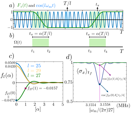
Figure 1: a) Modulation function $F_{z}(t)$ (green line) and its $l$th Fourier component $\cos(l\omega_{\rm m}t)$ (in blue) for $l=27$. Superimposed (shaded in green) the MW pulses width. Shaded in blue it is shown one period, $T/l$, of $\cos(l\omega_{\rm m}t)$, $T$ being the period of $F_{z}(t)$. b) MW pulses (in green) where it can be seen the relation between the pulse width $t_{\pi}$, and the period of $\cos(l\omega_{\rm m}t)$. In this case we have $\alpha=4$. c) Decay of the $f_{k}(\alpha)$ coefficients with $\alpha$ for $l=25$ (blue), $27$ (green), and $29$ (yellow). We highlight the value of $f_{27}(1)$ that is used in the next plot. d) Expectation value of the NV $\sigma_{x}$ operator evolving under Hamiltonian (2) with $B_{z}=2$ T and $\vec{A}=(2\pi)\times[19.12,55.21,-96.82]$ kHz. We applied 1120 $\pi$-pulses (final evolution time $t_{f}\approx 177\ \mu$s). The blue line is the signal for ideal instantaneous pulses with large contrast corresponding to $f_{27}(0)=-\frac{4}{27\pi}\approx-0.0472$, i.e. $\alpha=0.$ The green line corresponds to $\alpha=1$ (we simulated top-hat $\pi$-pulses with $\Omega\approx(2\pi)\times 42$ MHz, leading to $f_{27}(1)=-0.0157$) which yields to a reduced contrast. Violet panel is the theoretical prediction of $\langle\sigma_{x}\rangle_{t_{f}}=\cos{[f_{k}(\alpha)A^{\perp}_{x}t_{f}/4]}$ for $f_{27}(1)$ (i.e. $k=27$ and $\alpha=1$), blue square is the prediction for instantaneous $\pi$-pulses ($\langle\sigma_{x}\rangle_{t_{f}}=\cos{[f_{27}(0)A^{\perp}_{x}t_{f}/4]}$).

III Signal reduction

For the common case of top-hat pulses, the value of each $f_{l}$ coefficient for the elementary block in Fig. 1 a) is

$$f_{l} = \frac{2}{T}\big{[}\int_{0}^{t_{1}}\cos{(l\omega_{\rm m}s)}\ ds+\int_{t_{1}}^{t_{2}}\cos{[\Omega(s-t_{1})]}\cos{(l\omega_{\rm m}s)}\ ds$$ (7)

$$-\int_{t_{2}}^{t_{3}}\cos{(l\omega_{\rm m}s)}\ ds-\int_{t_{3}}^{t_{4}}\cos{[\Omega(s-t_{3})]}\cos{(l\omega_{\rm m}s)}\ ds$$

$$+\int_{t_{4}}^{T}\cos{(l\omega_{\rm m}s)}\ ds\big{]},$$

where $t_{2}-t_{1}=t_{4}-t_{3}\equiv t_{\pi}$ are the lengths of the $\pi$-pulses, see Fig. 1 a). For instantaneous $\pi$-pulses, $t_{\pi}=0$, the integrals $\int_{t_{1}}^{t_{2}}\cos{[\Omega(s-t_{1})]}\cos{(l\omega_{\rm m}s)}\ ds$ and $\int_{t_{3}}^{t_{4}}\cos{[\Omega(s-t_{1})]}\cos{(l\omega_{\rm m}s)}\ ds$ in Eq. (7) vanish, and $|f_{l}|=|\frac{4}{\pi l}|$ for odd $l$, and $|f_{l}|=0$ for even $l$. When $t_{\pi}$ is non-negligible one finds

$$f_{l}\equiv f_{l}(\alpha) = \frac{4(-1)^{(l+1)/2}\cos{(\alpha\pi)}}{(4\alpha^{2}-1)l\pi},$$ (8)

which implies that the sensitivity under a finite-width pulse sequence decreases as $\alpha^{-2}$, where $\alpha$ equals the length of $t_{\pi}=\alpha(T/l)$ measured in terms of the number of nuclear Larmor periods, Fig. 1 b). If we aim for a resonance at a certain $l$th harmonic we need to set $T=2\pi l/\omega_{n}$ (equivalent to the resonance condition $l\omega_{\rm m}=\omega_{\rm n}$) where $\omega_{n}$, grows linearly with the applied magnetic field $B_{z}$. Regarding the latter, note that according to the expressions in Appendix A we have $\omega_{n}=|\vec{\omega}_{n}|$ where $\vec{\omega}_{n}=(-\frac{1}{2}A_{x},-\frac{1}{2}A_{y},\omega_{\rm L}-\frac{1}{2}A_{z})$ and $\omega_{\rm L}=\gamma_{n}B_{z}$. Then, we have $\omega_{n}\approx\omega_{\rm L}-\frac{1}{2}A_{z}$, and for the case of large $B_{z}$ fields the behaviour of the resonance frequency $\omega_{n}$ can be well approximated by $\gamma_{n}B_{z}$.

From Eq. (1) we have $t_{\pi}=\pi/{\Omega}$, hence we have

$$\Omega=\frac{\pi}{\alpha}\frac{l}{T}\approx\frac{\gamma_{n}B_{z}}{2\alpha},$$ (9)

where we have used that $T=2\pi l/\omega_{n}$ and that, for large $B_{z}$ fields, $\omega_{n}\approx\gamma_{n}B_{z}$. Equation (9) implies for $B=2$ T ($5$ T), a proton nuclear spin as a target ($\gamma_{n}\equiv\gamma_{\rm H}=(2\pi)\times 42.57$ MHz/T), and a peak power limited by a maximum achievable value for $\Omega$, namely $\Omega=(2\pi)\times 10$ MHz, that $\alpha\approx 4.26\ (10.65)$. Note that, the peak power is $\propto\Omega^{2}$ while average power is $\propto\Omega$, in this respect see Supplemental Material Supplemental .

In Figure 1 c) we show the rapid decay of $f_{l}(\alpha)$ coefficients with $\alpha$, for $l=25$ (blue), $27$ (green), and $29$ (yellow) dictated by Eq. (8). In Fig. 1 d) we have computed the spectrum of a problem involving an NV center and a H nucleus for two values of $\Omega$ with $B_{z}=2$ T (see caption for details). In addition, with Hamiltonian (3) one can predict that, under the resonance condition, and assuming $\rho_{0}=\frac{1}{4}(\mathbb{I}+\sigma_{x})\otimes\mathbb{I}$ as the initial state of the NV-nucleus system (i.e. the NV is initialised in an equal superposition of the $|0\rangle$ and $|1\rangle$ states, and the nucleus is in a thermal state) the measured signal, i.e. the NV coherence, is

$$\langle\sigma_{x}\rangle_{t_{f}}=\frac{1}{4}{\rm Tr}\bigg{[}\rho_{0}\ e^{if_{k}(\alpha)A^{\perp}_{x}t_{f}/4\sigma_{z}\sigma_{x}}\ (\sigma_{x}\otimes\mathbb{I})\bigg{]}=\cos[f_{k}(\alpha)A^{\perp}_{x}t_{f}/4].$$ (10)

with $t_{f}$ the final time of the sequence. In Fig 1 d), the vertical violet line corresponds to the theoretically predicted resonance according Eq. (10) and we can observe how it matches with the numerically computed signal depth (green curve) for a finite value of the MW Rabi frequency at the resonance position $\omega_{\rm m}=\omega_{n}/27$. The blue square in the same figure is the signal depth for instantaneous pulses (i.e. at infinite MW power) corresponding to use $f_{27}(0)$ in Eq. (10). It is noteworthy to mention that, to take into account different effects as finite-width pulses as well as the presence of different rotating axes in the applied $\pi$-pulses (see next section), the numerical simulations in this article have been performed starting from Hamiltonian (16) in Appendix A. This Hamiltonian only assumes the elimination of fast counter rotating terms, of the order of GHz, on the MW driving as well as the presence of the third NV spin level which is detuned by a similar frequency amount of the order of GHz. For more details, see Eq. (16) and the paragraph below in Appendix A.

Hence, we can conclude that if an experiment is conducted at high $B_{z}$ (which implies large $\alpha$ to compensate for limited $\Omega$) the obtained signal gets dramatically reduced due to the decay of each $f_{l}(\alpha)$ with the $\alpha$ parameter.

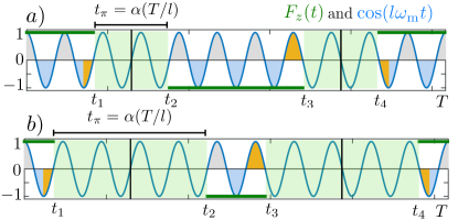
Figure 2: $F_{z}(t)$ and $\cos{(l\omega_{\rm m}t)}$ for two different pulse widths (shaded in green). a) $t_{\pi}=2(T/l)$ and b) $t_{\pi}=4(T/l)$, in both cases $l=11$. In the $\pi$-pulse regions it is remarked the center of each finite-width $\pi$-pulse with a vertical black line. The latter would correspond with the locations of the instantaneous $\pi$-pulses. The areas in yellow contribute to the value of $f_{l}$, while grey areas (positive oscillations) are cancelled by blue areas (negative oscillations).

IV Shaped $\pi$-pulses

If we measure the signal at a certain $l$th harmonic of $F_{z}(t)$ the length of the $\pi$-pulses may extend over many Larmor periods as long as the extended $\pi$-pulse action equals that of an instantaneous pulse. This can be seen in Fig. 2, where $F_{z}(t)$ (green flat lines), $\cos{(l\omega_{\rm m}t)}$ (solid blue lines) for $l=11$, and two possible time intervals used for the $\pi$-pulses (shaded in green panels) are shown. Specifically in Fig. 2 a) $t_{\pi}=2(T/l)$, while in b) $t_{\pi}=4(T/l)$. Then, if one assumes that the integral of $f_{l}$ could be written as

$$f_{l} = \frac{2}{T}\int_{0}^{T}F(s)\cos{(l\omega_{\rm m}s)}\ ds$$ (11)

$$= \frac{2}{T}\bigg{[}\int_{0}^{t_{1}}\cos{(l\omega_{\rm m}s)}\ ds-\int_{t_{2}}^{t_{3}}\cos{(l\omega_{\rm m}s)}\ ds$$

$$+ \int_{t_{4}}^{T}\cos{(l\omega_{\rm m}s)}\ ds\bigg{]},$$

i.e. without any contribution of the regions containing the $\pi$-pulses (see next paragraph for an explicit construction that will allow us having $f_{l}$ coefficients of the form that appears in Eq. 11) both cases in Figs. 2 a) and b) would lead to the same ideal value $|f_{l}|=|\frac{4}{\pi l}|$ as opposed to Eq. (8). This is because when $\pi$-pulses contain a natural number of periods of $\cos{(l\omega_{\rm m}t)}$ the latter expression of $f_{l}$ is reduced to the integral of yellow areas in Figs. 2, which are equal for a) and b). This offers the opportunity to extend their length until $t_{\pi}=(l-1)/2(T/l)$ and the potential to significantly reduce the Rabi frequency and hence the MW power.

Now, by substituting top-hat pulses for appropriately shaped pulses we can recover the ideal $|f_{l}|=|\frac{4}{\pi l}|$ scaling. This gains a factor of $\alpha^{2}$ in sensitivity and allows for a significant reduction in the power requirements of the pulsed schemes. To this end we consider the shaped $\pi$-pulse Hamiltonian as

$$H_{p}=\frac{\Omega(t)}{2}(|1\rangle\langle 0|e^{i\phi}+|0\rangle\langle 1|e^{-i\phi})=\frac{\Omega(t)}{2}\sigma_{\phi},$$ (12)

and a pulse width equal to a natural number of oscillations of $\cos{(l\omega_{\rm m}t)}$.

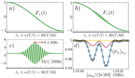
Figure 3: a) $F_{z}(t)$ in the $\pi$-pulse region after the application of a constant $\Omega$, while in b) we can observe the oscillating character of $F_{z}(t)$ because of the action of $\Omega(t)$ in c). The latter is displayed over $t_{\pi}=30(T/63)\approx 0.469\ \mu$s, i.e. $\alpha=30$ and $l=63$. We selected $c=t_{\pi}/10$. The maximum value of $\Omega(t)$ is $\approx(2\pi)\times 6.4$ MHz. d) Spectrum for ideal instantaneous pulses (blue), shaped pulses (squares), and top-hat pulses with a constant $\Omega$ of $(2\pi)\times 20$ MHz (yellow line) and $(2\pi)\times 40$ MHz (red line).

In the rotating frame of $H_{p}$, a $\sigma_{z}$ electronic operator evolves, for the first shaped $\pi$-pulse, as $\sigma_{z}\rightarrow\cos{\bigg{[}\int_{t_{1}}^{t}\Omega(s)\ ds\bigg{]}}\sigma_{z}+\sin{\bigg{[}\int_{t_{1}}^{t}\Omega(s)\ ds\bigg{]}}\sigma_{\phi}^{\perp}$, where $t<t_{1}+t_{\pi}\equiv t_{2}$, and $\sigma_{\phi}^{\perp}=-i(|1\rangle\langle 0|e^{i\phi}-|0\rangle\langle 1|e^{-i\phi})$. This description is similar for any other shaped $\pi$-pulse of the sequence by simply replacing $t_{1}$ by $t_{j}$, the latter being the initial time of the $j$th shaped $\pi$-pulse. Now we focus only on the part containing the $\sigma_{z}$ operator, i.e. the one leading to the $F_{z}(t)\equiv\cos{\big{[}\int_{t_{j}}^{t_{j+1}}\Omega(s)\ ds\big{]}}$ modulation function, because the $\sigma_{\phi}^{\perp}$ component leads to the $F_{x}(t)$ and $F_{y}(t)$ modulation functions that do not contribute to the spectrum if the sequence contains pulses over different directions Haase16 ; Lang17 . Then, we have to find a $\Omega(s)$ that minimise, in the shaped $\pi$-pulse region, the overlap between $F_{z}(t)$ and $\cos{(l\omega_{\rm m}t)}$, this is

$$\int_{t_{j}}^{t_{j+1}}F_{z}(u)\ \cos{\big{(}l\omega_{\rm m}u\big{)}}\ du=0,$$ (13)

with $t_{j+1}-t_{j}=t_{\pi}$. In addition, in order to have a continuous $F_{z}(t)$ the following boundary conditions are needed: $F_{z}(t_{j})=(-1)^{n+1}\ \ {\rm and}\ \ F_{z}(t_{j+1})=(-1)^{n}$, for the $n$th shaped $\pi$-pulse.

These conditions have an infinite number of solutions and here we present as an example the analytical solution

$$F_{z}(u)=\cos{\bigg{[}\frac{\pi}{t_{\pi}}(u-t_{j})\bigg{]}}-\beta e^{-\frac{(u-t_{p})^{2}}{2c^{2}}}\sin{\bigg{[}\frac{2\pi\alpha}{t_{\pi}}(u-t_{j})\bigg{]}},$$ (14)

with $\beta$ a parameter that will be fixed with Eq. (13). For the first shaped $\pi$-pulse $t_{p}$ is the middle point in between $t_{1}$ and $t_{2}$, or between $t_{3}$ and $t_{4}$ for the second one. The $\alpha$ and $c$ parameters can be advisedly adjusted, such that their value determine the pulse length and maximum intensity of the employed $\Omega(t)$ in Eq. (12). The above solution is valid for $\alpha$ equal to $1,2,3,..$ i.e. when the shaped $\pi$-pulse contains a natural number of periods of $\cos{(l\omega_{\rm m}t)}$. Equation (13) leads to the following condition for $\beta$ (see Appendix C)

$$\beta=\frac{4\sqrt{2}\gamma\alpha}{(4\alpha^{2}-1)\pi^{3/2}}/\big{[}1-\exp{\big{(}\frac{-8\alpha^{2}\pi^{2}}{\gamma^{2}}\big{)}}\big{]}$$ (15)

where $\gamma$ and $c$ are related as $\gamma=t_{\pi}/c$. Once $\beta$ is chosen, one can calculate $\Omega(t)=\partial_{t}\arccos{[F(t)]}$ from $F_{z}(t)=\cos{\big{[}\int_{t_{j}}^{t_{j+1}}\Omega(s)\ ds\big{]}}$.

Fig. 3 a) shows the evolution of $F_{z}(t)$ from $+1$ to $-1$ that results from the application of a $\pi$-pulse with a constant $\Omega$, i.e. a standard top-hat pulse as those in Fig. 1 b), while Fig. 3 b) corresponds to $F_{z}(t)$ for the shaped $\pi$-pulse whose $\Omega(t)$ is shown in c). To further visualise the effect of the modulated Rabi frequency $\Omega(t)$ in the $F_{z}(t)$ function, in the Supplemental Material Supplemental we have included a whole period of $F_{z}(t)$ that results from the application of the $\Omega(t)$ in Fig. 3 c). In Fig. 3 d) we have computed the response versus frequency that results from a system at $B_{z}=1.5$ T involving a NV center and two H nuclei with $\vec{A}_{1}=(2\pi)\times[0,14.43,-46.63]$ kHz and, $\vec{A}_{2}=(2\pi)\times[-10.93,6.31,-42.34]$ kHz. The blue line corresponds to the signal obtained for $1440$ ideal instantaneous $\pi$-pulses (final time of the sequence $t_{f}\approx 0.71$ ms). The black squares represent the signal that emerges when our shaped pulses in Fig. 3 c) are applied. Here we use the sequence [XYXYYXYX]^N for its robustness against errors on the MW control (for an analysis including non-robust pulse constructions see Suplemental Material Supplemental ) with $N=180$ and X (Y) a shaped pulse with phase $\phi=0$ ($\phi=\frac{\pi}{2}$), see Eq. (12). This signal overlaps with the ideal one employing instantaneous $\pi$-pulses which demonstrates the efficiency of our method. At this point it is important to clarify that the previous numerical simulation involving NV nuclei has been computed from Eq. (16) replacing the driving in that equation by the pulse Hamiltonian in Eq. (12). The yellow line corresponds to the application of standard top-hat $\pi$-pulses with $\Omega=(2\pi)\times 20$ MHz, while the red one uses $\Omega=(2\pi)\times 40$ MHz. In these two cases, the signal contrast is seriously reduced with respect to the one obtained with our shaped pulses which employ a maximum of only $\Omega=(2\pi)\times 6.4$ MHz.

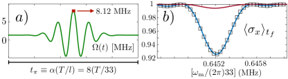
Figure 4: Our method applied to a classical signal of the form $B_{s}[\cos{(\omega_{s_{1}}t)}+\cos{(\omega_{s_{2}}t)}]$ with $\omega_{s_{1,2}}=(2\pi)\times(21.288,21.295)$ MHz, and $B_{s}=0.2$ G. The modulated Rabi frequency in a) leads to a signal in b) (squares) that overlaps with the ideal signal obtained with instantaneous $\pi$-pulses (blue line). We used $\alpha=8$ and $c=t_{\pi}/10$. The red line in b) uses top-hat $\pi$-pulses with $\Omega=(2\pi)\times 10$ MHz.

In Fig. 4 the same effect is shown for a classical signal target. Here we demonstrate that the contrast reduction appears even at not so high $B_{z}$ fields (note we used a classical signal with frequencies corresponding to H nuclei at $B_{z}\approx 0.5$ T). In this respect, by inspecting Eq. (9) it gets clear that finding a non negligible value for $\alpha$, which leads to a reduced $f_{l}(\alpha)$, depends on the ratio between $B_{z}$ and $\Omega$. Hence, if the MW source cannot deliver high power, i.e. only low values of $\Omega$ are accesible, we get poor signal contrast. However, the application of our shaped $\pi$-pulses leads to an undistinguishable signal (squares) with respect to the ideal spectrum (blue line). The red line with poor contrast has been computed with top hat pulses corresponding to $\Omega=(2\pi)\times 10$ MHz. We used the same $[{\rm XYXYYXYX}]^{N}$ sequence for $N=5$. That is 40 pulses, shaped and top-hat, have been applied. The final time of the sequence is $t_{f}\approx 0.03$ ms and shaped pulses are generated with a maximum of $\Omega=(2\pi)\times 8.12$ MHz.

Finally, we want to remark that in order to achieve similar results to the ideal case in Fig. 3 d) with finite top-hat pulses, a value for $\Omega$ of, at least, $\Omega=(2\pi)\times 100$ MHz is needed. This is much larger than the maximum of $\Omega(t)$ in Fig. 3 c) which implies that our method requires a much lower peak power. More specifically, the square ratio (peak power ratio) of these two quantities is $[(2\pi)\times 100/(2\pi)\times 6.4]^{2}\approx 244$. In addition, the ratio between the average energy required by the two approaches is $E_{[\pi-\rm pulse]}^{\rm top-hat}/E_{[\pi-\rm pulse]}^{\rm shaped}=27.47$ (see Supplemental Material Supplemental for a derivation of the standard expressions for the $\pi$-pulse average energies) which certifies that our method is energy efficient. A similar situation occurs in Fig. 4. Here for obtaining the same contrast as in the ideal case, top-hat pulses require at least $\Omega=(2\pi)\times 50$ MHz, larger than the maximum value of $\Omega(t)$ in Fig.4 a). This leads a peak power ratio $\approx 38$ while $E_{[\pi-\rm pulse]}^{\rm top-hat}/E_{[\pi-\rm pulse]}^{\rm shaped}=10.63$.

V Conclusions

We have considered quantum sensing experiments at high magnetic fields that lead to high frequency signals and demonstrated that the finite length of standard top-hat pulses in dynamical decoupling sequences lead to a rapid decrease of sensitivity with signal frequency. We present a general solution to this problem which allows to significant reductions in the required microwave power. Our method is general and applicable to any magnetic defect.

VI acknowledgments

This work was supported by the ERC Synergy grant BioQ (grant no 319130), the EU STREP project HYPERDIAMOND and the DFG CRC 1279. The authors acknowledge support by the state of Baden-Württemberg through bwHPC and the German Research Foundation (DFG) through grant no INST 40/467-1 FUGG. J. C. acknowledges Universität Ulm for a Forschungsbonus.

Appendix A NV-nucleus Hamiltonian

The Hamiltonian (1) in the rotating frame of the electron-spin free-energy term, $DS_{z}^{2}-\gamma_{e}B_{z}S_{z}$, reads

$$H=-\omega_{n}\ \hat{\omega}_{n}\cdot\vec{I}+\frac{1}{2}\sigma_{z}\ \vec{A}\cdot\vec{I}+\frac{\Omega}{2}(|1\rangle\langle 0|e^{i\phi}+|0\rangle\langle 1|e^{-i\phi}).$$ (16)

Here, we have eliminated any electron spin component containing the $|-1\rangle$ state because, as the MW driving is tuned with the $|0\rangle\leftrightarrow|1\rangle$ transition, the $|-1\rangle$ component gets no populated as well as fast counter rotating terms of the MW driving. In this manner, and as it is commented in the text, we will use this Hamiltonian as the starting point for our numerical simulations. The $\vec{\omega}_{n}$ vector is $\vec{\omega}_{n}=(-\frac{1}{2}A_{x},-\frac{1}{2}A_{y},\omega_{\rm L}-\frac{1}{2}A_{z})$, with $\vec{A}=\frac{\mu_{0}\gamma_{e}\gamma_{n}}{2|\vec{r}|^{3}}[\hat{z}-3\frac{(\hat{z}\cdot\vec{r})\vec{r}}{|\vec{r}|^{2}}]$ being the hyperfine vector (note that we are assuming dipole-dipole interactions between the NV and the nuclear spin) $\omega_{n}=|\vec{\omega}_{n}|$ is the resonance frequency of the nucleus which is shifted from the Larmor frequency because of the hyperfine field, and $\hat{\omega}_{n}=\vec{\omega}_{n}/\omega_{n}$.

In a new rotating frame with respect to (w.r.t.), both, $-\omega_{n}\ \hat{\omega}_{n}\cdot\vec{I}$ and to the MW driving, one can find that

$$H=\frac{F_{z}(t)\sigma_{z}}{2}\vec{I}\cdot\bigg{[}(\vec{A}-\vec{A}\cdot\hat{\omega}_{n}\hat{\omega}_{n})\cos{(\omega_{n}t)}+\hat{\omega}_{n}\times\vec{A}\sin{(\omega_{n}t)}+\vec{A}\cdot\hat{\omega}_{n}\hat{\omega}_{n}\bigg{]},$$ (17)

where $F_{z}(t)$ is the modulation function, see Lang17 , that appears as a consequence of the applied $\pi$-pulses. As $F_{z}(t)$ will alternate between $+1$ and $-1$ the constant term $\vec{A}\cdot\hat{\omega}_{n}\hat{\omega}_{n}$ can be averaged out. Then, the above Hamiltonian can be written as

$$H=\frac{F_{z}(t)}{2}\ \sigma_{z}\bigg{[}A^{\perp}_{x}I_{x}\cos{(\omega_{n}t)}+A^{\perp}_{y}I_{y}\sin{(\omega_{n}t)}\bigg{]},$$ (18)

where $A^{\perp}_{x}=|\vec{A}-\vec{A}\cdot\hat{\omega}_{n}\hat{\omega}_{n}|=A^{\perp}_{y}=|\hat{\omega}_{n}\times\vec{A}|$, the $\hat{x}$ and $\hat{y}$ directions are $\hat{x}=(\vec{A}-\vec{A}\cdot\hat{\omega}_{n}\hat{\omega}_{n})/A^{\perp}_{x}$, $\hat{y}=\hat{\omega}_{n}\times\vec{A}/A^{\perp}_{y}$, and $I_{x}=\vec{I}\cdot\hat{x}$, $I_{y}=\vec{I}\cdot\hat{y}$. In this manner, Eq (18) coincides with Hamiltonian (2).

Appendix B The case of a classical field

If we want to detect classical signals of the form $\vec{B}_{\rm s}\cos{(\omega_{\rm s}t)}$, instead of the initial Hamiltonian in Eq. (1), we have to consider

$$H=DS_{z}^{2}-\gamma_{e}B_{z}S_{z}+\Omega_{\rm s}S_{z}\cos{(\omega_{\rm s}t)}+\sqrt{2}\Omega S_{x}\cos(\omega t-\phi),$$ (19)

where the target signal Rabi frequency is $\Omega_{\rm s}=\gamma_{e}\vec{B}_{\rm s}\cdot\hat{z}$. The other components ($\hat{x}$ and $\hat{y}$) of the classical signal field $\vec{B}_{\rm s}\cos{(\omega_{\rm s}t)}$ can be averaged out because $\omega_{\rm s}$ is not on resonance with any of the two possible NV electron spin transitions. More specifically, if we assume that $\vec{B}_{\rm s}\cos{(\omega_{\rm s}t)}$ is generated by a spin cluster, $\omega_{\rm s}$ would be on the range of several MHz for $B_{z}$ around a few teslas, while NV transitions require several the Gigahertz to be excited.

In the rotating frame of $DS_{z}^{2}+|\gamma_{e}|B_{z}S_{z}$ and setting on resonance the driving frequency $\omega$ with, for example, the $|0\rangle\leftrightarrow|1\rangle$ transition, we have

$$H=\frac{\Omega_{s}}{2}\sigma_{z}\cos{(\omega_{\rm s}t)}+\frac{\Omega}{2}(|1\rangle\langle 0|e^{i\phi}+|0\rangle\langle 1|e^{-i\phi}),$$ (20)

once we have eliminated constants and any term including the $|-1\rangle$ NV spin component. The use of a standard scheme, as the Hartmann-Hahn double resonance condition Hartmann62 , to make interact the NV with the classical field is limited to low values of $\omega_{s}$. This is because it is required to hold $\omega_{s}=\Omega$ and the driving power, here reflected in the value of $\Omega$, could be limited. The latter can be easily seen by noting that, in a rotating frame with respect to $\frac{\Omega}{2}(|1\rangle\langle 0|+|0\rangle\langle 1|)$ where we set $\phi=0$ and $\Omega$ is constant, the above Hamiltonian is

$$H=\frac{\Omega_{s}}{4}(|+\rangle\langle-|e^{i\Omega t}+|-\rangle\langle+|e^{-i\Omega t})(e^{i\omega_{s}t}+e^{-i\omega_{s}t}).$$ (21)

where $|\pm\rangle=\frac{1}{\sqrt{2}}(|\uparrow\rangle\pm i|\downarrow\rangle)$. Now one can see that, unless the condition $\Omega=\omega_{s}$ holds, the previous Hamiltonian is entirely time-dependent and would average to zero because of the rotating wave approximation.

Hence, one should consider the use of pulsed schemes. In this case, Eq. (20) can be written in the rotating frame of the MW driving $\frac{\Omega}{2}(|1\rangle\langle 0|e^{i\phi}+|0\rangle\langle 1|e^{-i\phi})$ with $\Omega$ applied stroboscopically, as

$$H=\frac{\Omega_{s}}{2}F_{z}(t)\sigma_{z}\cos{(\omega_{s}t)}.$$ (22)

Now, as $F_{z}(t)=\sum_{l}f_{l}\cos{(l\omega_{\rm m}t)}$, and in the case of $k\omega_{\rm m}=\omega_{s}$ (i.e. resonance condition for the $k$th harmonic) the above Hamiltonian after eliminating fast rotating terms is

$$H=\frac{\Omega_{s}}{4}f_{k}\ \sigma_{z},$$ (23)

which is Eq. (6).

Appendix C Integrating $F_{z}(u)$

The condition in Eq. (13) when applied to the solution in Eq. (14) leads to the two following integrals

$$\int_{t_{1}}^{t_{2}}\cos{\bigg{[}\frac{\pi}{t_{\pi}}(u-t_{1})\bigg{]}}\ \cos{\bigg{[}k\frac{2\pi}{T}u\bigg{]}}\ du$$ (24)

$$= t_{\pi}\bigg{[}\frac{1}{(2\alpha+1)\pi}+\frac{1}{(2\alpha-1)\pi}\bigg{]},$$

and

$$\int_{t_{1}}^{t_{2}}\exp{\bigg{[}-\frac{(u-t_{p})^{2}}{2c^{2}}\bigg{]}}\sin{\bigg{[}\frac{2\pi\alpha}{t_{\pi}}(u-t_{1})\bigg{]}}\ \cos{\bigg{[}k\frac{2\pi}{T}u\bigg{]}}\ du$$ (25)

$$\approx c\sqrt{\frac{\pi}{2}}\bigg{[}1-\exp{\bigg{(}\frac{-8\alpha^{2}\pi^{2}}{\gamma^{2}}\bigg{)}}\bigg{]}$$

with $c=\frac{t_{\pi}}{\gamma}$. Note that for solving the last integral we have used the following relations

$$\int_{-\infty}^{+\infty}e^{-(x-b)^{2}/2c^{2}}dx=\sqrt{2}|c|\sqrt{\pi}$$

$$\int_{-\infty}^{+\infty}e^{-ax^{2}}\cos{(bx)}dx=\sqrt{\frac{\pi}{a}}e^{-b^{2}/4a}.$$ (26)

References

- (1) I. I. Rabi, J. R. Zacharias, S. Millman, and P. Kusch, A New Method of Measuring Nuclear Magnetic Moment, Phys. Rev. 53, 318 (1938).
- (2) R.R. Ernst, G. Bodenhausen, and A. Wokaun, Principles of Nuclear Magnetic Resonance in One and Two Dimensions, Oxford Science Publications (1987).
- (3) M. Findeisen and S. Berger, 50 and More Essential NMR Experiments: A Detailed Guide, Wiley-VCH, Weinheim, (2014).
- (4) S. Schmitt, T. Gefen, F. M. Stürmer, T. Unden, G. Wolff, Ch. Müller, J. Scheuer, B. Naydenov, M. Markham, S. Pezzagna, J. Meijer, I. Schwarz, M. B. Plenio, A. Retzker, L. P. McGuinness, and F. Jelezko, Submillihertz magnetic spectroscopy performed with a nanoscale quantum sensor, Science 351, 832 (2017).
- (5) J.M. Boss, K.S. Cujia, J. Zopes, and C.L. Degen, Quantum sensing with arbitrary frequency resolution, Science 351, 837 (2017).
- (6) D.R. Glenn, D.B. Bucher, J. Lee, M.D. Lukin, H. Park and R.L. Walsworth, High-resolution magnetic resonance spectroscopy using a solid-state spin sensor, Nature 555, 351 (2018).
- (7) M. H. Levitt, Spin dynamics: Basics of nuclear magnetic resonance (Wiley, 2008).
- (8) Y. Wu, F. Jelezko, M. B. Plenio, and T. Weil, Diamond Quantum Devices in Biology, Angew. Chem. Int. Ed. 55, 6586 (2016).
- (9) M. W. Doherty, N. B. Manson, P. Delaney, F. Jelezko, J. Wrachtrup, and L. C. L. Hollenberg, The nitrogen-vacancy colour centre in diamond, Phys. Rep. 528, 1 (2013).
- (10) V.V. Dobrovitski, G.D. Fuchs, A.L. Falk, C. Santori, and D.D. Awschalom, Quantum Control over Single Spins in Diamond, Annu. Rev. Condens. Matter Phys 4, 23 (2013).
- (11) S. Kolkowitz, Q. P. Unterreithmeier, S. D. Bennett, and M. D. Lukin, Sensing Distant Nuclear Spins with a Single Electron Spin, Phys. Rev. Lett. 109, 137601 (2012).
- (12) T. H. Taminiau, J. J. T. Wagenaar, T. van der Sar, F. Jelezko, V. V. Dobrovitski, and R. Hanson, Detection and Control of Individual Nuclear Spins Using a Weakly Coupled Electron Spin, Phys. Rev. Lett. 109, 137602 (2012).
- (13) N. Zhao, J. Honert, B. Schmid, M. Klas, J. Isoya, M. Markham, D. Twitchen, F. Jelezko, R.-B. Liu, H. Fedder, and J. Wrachtrup, Sensing single remote nuclear spins, Nat. Nanotechnol. 7, 657 (2012).
- (14) C. Müller, X. Kong, J.-M. Cai, K. Melentijević, A. Stacey, M. Markham, D. Twitchen, J. Isoya, S. Pezzagna, J. Meijer, J. F. Du, M. B. Plenio, B. Naydenov, L. P. McGuinness, and F. Jelezko, Nuclear magnetic resonance spectroscopy with single spin sensitivity, Nat. Commun 5, 4703 (2014).
- (15) I. Lovchinsky, A.O. Sushkov, E. Urbach, N. P. de Leon, S. Choi, K. De Greve, R. Evans, R. Gertner, E. Bersin, C. Müller, L. McGuinness, F. Jelezko, R. L. Walsworth, H. Park, M. D. Lukin, Nuclear magnetic resonance detection and spectroscopy of single proteins using quantum logic, Science 351, 836 (2016).
- (16) M. H. Abobeih, J. Cramer, M. A. Bakker, N. Kalb, M. Markham, D. J. Twitchen, and T. H. Taminiau, One-second coherence for a single electron spin coupled to a multi-qubit nuclear-spin environment, Nat. Commun. 9, 2552 (2018).
- (17) C. A. Ryan, J. S. Hodges, and D. G. Cory, Robust Decoupling Techniques to Extend Quantum Coherence in Diamond, Phys. Rev. Lett. 105, 200402 (2010).
- (18) B. Naydenov, F. Dolde, L.T. Hall, C. Shin, H. Fedder, L.C.L. Hollenberg, F. Jelezko, J. Wrachtrup, Dynamical decoupling of a single-electron spin at room temperature, Phys. Rev. B 83, 081201(R) (2011).
- (19) A. M. Souza, G. A. Álvarez, and D. Suter, Robust dynamical decoupling, Phil.Trans. R. Soc. A 370, 4748 (2012).
- (20) M. V. Gurudev Dutt, L. Childress, L. Jiang, E. Togan, J. Maze, F. Jelezko, A. S. Zibrov, P. R. Hemmer, and M. D. Lukin, Quantum Register Based on Individual Electronic and Nuclear Spin Qubits in Diamond, Science 316, 1312 (2007).
- (21) L. Robledo, L. Childress, H. Bernien, B. Hensen, P. F. A. Alkemade, and R. Hanson, High-fidelity projective read-out of a solid-state spin quantum register, Nature 477, 574 (2011).
- (22) T. van der Sar, Z. H. Wang, M. S. Blok, H. Bernien, T. H. Taminiau, D. M. Toyli, D. A. Lidar, D. D. Awschalom, R. Hanson, and V. V. Dobrovitski, Decoherence-protected quantum gates for a hybrid solid-state spin register, Nature 484, 82 (2012).
- (23) G.-Q. Liu, H. C. Po, J. Du, R.-B. Liu, and X.-Y. Pan, Noise-resilient quantum evolution steered by dynamical decoupling, Nat. Commun. 4, 2254 (2013).
- (24) T. H. Taminiau, J. Cramer, T. van der Sar, V. V. Dobrovitski, and R. Hanson, Universal control and error correction in multi-qubit spin registers in diamond, Nat. Nanotechnol. 9, 171 (2014).
- (25) G. Waldherr, Y. Wang, S. Zaiser, M. Jamali, T. Schulte- Herbrüggen, H. Abe, T. Ohshima, J. Isoya, J. F. Du, P. Neumann, and J. Wrachtrup, Quantum error correction in a solid-state hybrid spin register, Nature 506, 204 (2014).
- (26) B. Hensen, H. Bernien, A. E. Dréau, A. Reiserer, N. Kalb, M. S. Blok, J. Ruitenberg, R. F. L. Vermeulen, R. N. Schouten, C. Abellán, W. Amaya, V. Pruneri, M. W. Mitchell, M. Markham, D. J. Twitchen, D. Elkouss, S. Wehner, T. H. Taminiau, and R. Hanson, Loophole-free Bell inequality violation using electron spins separated by 1.3 kilometres, Nature 526, 682 (2015).
- (27) J. Cramer, N. Kalb, M. A. Rol, B. Hensen, M. S. Blok, M. Markham, D. J. Twitchen, R. Hanson, and T. H. Taminiau, Repeated quantum error correction on a continuously encoded qubit by real-time feedback, Nat. Commun. 7, 11526 (2016).
- (28) P. Neumann, J. Beck, M. Steiner, F. Rempp, H. Fedder, P. R. Hemmer, J. Wrachtrup, and F. Jelezko, Single-Shot Readout of a Single Nuclear Spin, Science 329, 542 (2010).
- (29) E. C. Reynhardt and G. L. High, Nuclear magnetic resonance studies of diamond, Progress in Nuclear Magnetic Resonance Spectroscopy 38, 37 (2001).
- (30) S. Hartmann and E. Hahn, Nuclear Double Resonance in the Rotating Frame, Phys. Rev. 128, 2042 (1962).
- (31) J.-M. Cai, B. Naydenov, R. Pfeiffer, L. McGuinness, K. D. Jahnke, F. Jelezko, M. B. Plenio, an A. Retzker, Robust dynamical decoupling with concatenated continuous driving, New J. Phys. 14, 113023 (2012).
- (32) S. Pasini, T. Fischer, P. Karbach, and G. S. Uhrig, Optimization of short coherent control pulses, Phys. Rev. A 77, 032315 (2008).
- (33) S Pasini and G S Uhrig, Generalization of short coherent control pulses: extension to arbitrary rotations, J. Phys. A: Math. Theor. 41, 312005 (2008).
- (34) Z.-Y. Wang and R.-B. Liu, Protection of quantum systems by nested dynamical decoupling, Phys. Rev. A 83, 022306 (2011).
- (35) Q.-Y. Cao, Z.-J. Shu, P.-C. Yang, M. Yu, M.-S. Gong, J.-Y. He, R.-F. Hu, A. Retzker, M. B. Plenio, C. Müller, N. Tomek, B. Naydenov, L. P. McGuinness, F. Jelezko, and J.-M. Cai, Protecting quantum spin coherence of nanodiamonds in living cells, arXiv:1710.10744.
- (36) J. R. Maze, J. M. Taylor, and M. D. Lukin, Electron spin decoherence of single nitrogen-vacancy defects in diamond, Phys. Rev. B 78, 094303 (2008).
- (37) A. A. Maudsley, Modified Carr-Purcell-Meiboom-Gill sequence for NMR fourier imaging applications, J. Magn. Reson. 69, 488 (1986).
- (38) T. Gullion, D. B. Baker, and M. S. Conradi, New, compensated Carr-Purcell sequences, J. Magn. Reson. 89, 479 (1990).
- (39) A. M. Souza, G. A. Alvarez, and D. Suter, Robust Dynamical Decoupling for Quantum Computing and Quantum Memory, Phys. Rev. Lett. 106, 240501 (2011).
- (40) J. Casanova, Z.-Y. Wang, J. F. Haase, and M. B. Plenio, Robust dynamical decoupling sequences for individual-nuclear-spin addressing, Phys. Rev. A 92, 042304 (2015).
- (41) Z.-Y. Wang, J. F. Haase, J. Casanova, and M. B. Plenio, Positioning nuclear spins in interacting clusters for quantum technologies and bioimaging, Phys. Rev. B 93, 174104 (2016).
- (42) J. Casanova, Z.-Y. Wang, and M. B. Plenio, Noise-Resilient Quantum Computing with a Nitrogen-Vacancy Center and Nuclear Spins, Phys. Rev. Lett. 117, 130502 (2016).
- (43) Z.-Y. Wang, J. Casanova, and M. B. Plenio, Delayed entanglement echo for individual control of a large number of nuclear spins, Nat. Commun. 8, 14660 (2017).
- (44) J. Casanova, Z.-Y. Wang, and M. B. Plenio, Arbitrary nuclear-spin gates in diamond mediated by a nitrogen-vacancy-center electron spin, Phys. Rev. A 96, 032314 (2017).
- (45) J. F. Haase, Z.-Y. Wang, J. Casanova, and M. B. Plenio, Soft Quantum Control for Highly Selective Interactions among Joint Quantum Systems, Phys. Rev. Lett. 121, 050402 (2018).
- (46) Supplemental Material.
- (47) J. F. Haase, Z.-Y. Wang, J. Casanova, and M. B. Plenio, Pulse-phase control for spectral disambiguation in quantum sensing protocols, Phys. Rev. A 94, 032322 (2016).
- (48) J. E. Lang, J. Casanova, Z.-Y. Wang, M. B. Plenio, and T. S. Monteiro, Enhanced Resolution in Nanoscale NMR via Quantum Sensing with Pulses of Finite Duration, Phys. Rev. Applied 7, 054009 (2017).