Mixed aggregated finite element methods for the unfitted discretization of the Stokes problem

Abstract.

In this work, we consider unfitted finite element methods for the numerical approximation of the Stokes problem. It is well-known that this kind of methods lead to arbitrarily ill-conditioned systems. In order to solve this issue, we consider the recently proposed aggregated finite element method, originally motivated for coercive problems. However, the well-posedness of the Stokes problem is far more subtle and relies on a discrete inf-sup condition. We consider mixed finite element methods that satisfy the discrete version of the inf-sup condition for body-fitted meshes, and analyze how the discrete inf-sup is affected when considering the unfitted case. We propose different aggregated mixed finite element spaces combined with simple stabilization terms, which can include pressure jumps and/or cell residuals, to fix the potential deficiencies of the aggregated inf-sup. We carry out a complete numerical analysis, which includes stability, optimal a priori error estimates, and condition number bounds that are not affected by the small cut cell problem. For the sake of conciseness, we have restricted the analysis to hexahedral meshes and discontinuous pressure spaces. A thorough numerical experimentation bears out the numerical analysis. The aggregated mixed finite element method is ultimately applied to two problems with non-trivial geometries.

Keywords: Embedded boundary; unfitted finite elements; Stokes; inf-sup; conditioning.

1. Introduction

Unfitted finite element (FE) techniques are receiving increasing attention since they are very appealing in many practical situations. Such techniques avoid the generation of body-fitted meshes, which is a serious bottleneck in large scale simulations. They are particularly well-suited to multi-phase and multi-physics applications with moving interfaces (e.g., fracture mechanics, fluid-structure interaction [1], or free surface flows), and in applications with varying domains (e.g., shape or topology optimization frameworks, additive manufacturing and 3D printing simulations [2], stochastic geometry problems). Unfitted FE methods have been named in different ways. When designed for capturing interfaces, they are usually denoted as extended finite element method (XFEM) [3], whereas they are denoted as embedded, immersed, or unfitted methods when the motivation is to simulate a problem using a (usually simple) background mesh (see, e.g., the cutFEM method [4]).

Yet useful, unfitted FE methods have known drawbacks. They pose problems to numerical integration, imposition of Dirichlet boundary conditions, and lead to ill conditioned problems [5]. For most of the unfitted FE techniques, the condition number of the discrete linear system does not only depend on the characteristic element size of the background mesh, but also on the ratios for all cut cells of the total cell volume and the cell volume inside the physical domain, which can be arbitrarily small, leading to the so-called small cut cell problem. Methods based on fictitious material [6] require a penalty term that goes to zero with a power of the mesh size for optimal convergence and thus, are also affected by these problems. Preconditioned iterative linear solvers suitable for standard FE methods are not robust for these formulations. Recently, a robust domain decomposition preconditioner able to deal with cut cells has been proposed in [7] for first order methods, but these preconditioners still require some special treatment for the robust direct solution of local-to-subdomain systems.

The authors have recently proposed in [8] an unfitted FE formulation, referred to as the aggregated finite element method (agFEM), that fixes the ill conditioning issues associated with cut cells for elliptic partial differential equations. This novel method relies on the so-called aggregated finite element (agFE) spaces, grounded on cell aggregation techniques and judiciously chosen linear constraints for conflictive degrees of freedom with respect to interior ones. This approach can be applied to grad-conforming (globally continuous) spaces and discontinuous FE spaces of arbitrary order. The agFEM leads to a well-posed Galerkin formulation of elliptic problems, viz., no stabilization terms are needed and the method is thus consistent. Furthermore, the resulting linear system have condition numbers that scale only with the element size of the background mesh in the same way as in standard FE methods for body-fitted meshes. These methods have been implemented in FEMPAR, a large scale FE software package [9, 10].

Compared to other existing approaches, the most salient one is the ghost penalty formulation used in the CutFEM method [4, 11]. In any case, this approach leads to weakly non-consistent algorithms and requires to compute high order derivatives on faces for high order FEs, which are not at our disposal in general FE codes and are expensive to compute, certainly complicating the implementation of the methods and harming code performance. For B-spline approximations, one can consider the so-called extension or extrapolation techniques (see, e.g., [12, 13, 14]). These works are close to the agFEM [8] in the sense that the problematic DOFs associated with B-splines with small support inside the physical domain are eliminated by constraining them as a linear combination of well-posed DOFs. Such aggregation approaches are not new in discontinuous Galerkin (DG) methods (see, e.g., [15, 16, 17]), for which the situation is much easier, since no conformity must be kept. In fact, some aggregation techniques in DG [15, 16, 17] can be casted as discontinuous agFEMs.

The use of mixed FE methods on unfitted meshes has been explored in previous works. The combination of ghost penalty stabilization and inf-sup stable elements for the unfitted FE approximation of the Stokes problem was originally addressed in [18] for triangular meshes in two dimensions. The analysis therein relies on the continuous inf-sup condition on the interior domain, viz., the union of interior cells (not intersecting the boundary), in order to prove pressure stability in interior cells, whereas cut cell pressure stability relies on ghost penalty stabilization. The extension of this work to interface Stokes problems for the MINI element has been proposed in [19] (see also [20] for a similar strategy). It has been observed in [21] that the analysis of unfitted and XFEM FE methods, e.g., in [18, 19, 20], is not fully satisfactory, because it relies on the inf-sup condition of the interior domain, which has an inf-sup constant that depends on the mesh refinement and can tend to zero. Guzmán and Olshanskii follow a different approach in [21], proving stability and error estimates for some families of inf-sup stable elements on triangles and tetrahedra. We refer the reader to [18, 21] for more references on this subject in the frame of XFEM. As an alternative to mixed FE methods, globally stabilized residual-based and pressure jump first order schemes combined with ghost penalty stabilization have been used in [22]. Global residual-based stabilization has also been used in [13, 14] for B-spline approximations.

In this work, we propose to combine the agFEM approach, which fixes the small cut cell problem for the numerical approximation of elliptic PDEs, with mixed FE spaces. Unsurprisingly, the development of mixed agFE spaces that satisfy a discrete version of the inf-sup condition is not straightforward. The discrete inf-sup condition requires a perfect balance of the velocity and pressure spaces, whereas the boundary-cell intersections can be arbitrary, leading to a large set of possible cell aggregates geometries. In this work, we consider hexahedral meshes and arbitrary order mixed FE spaces with discontinuous pressures, and analyze the potential deficiencies of the unfitted inf-sup in terms of a set of improper aggregates and interfaces that will require additional stabilization. An abstract stability analysis under some assumptions about such stabilization allows us to define effective stabilization terms. We propose two algorithms. The first one combines a standard aggregated tensor-product Lagrangian FE with interior residual-based and pressure jump face stabilization on improper aggregates and faces, respectively. The second one makes use of an agFE space in terms of a serendipity-based extension of tensor-product Lagrangian FEs combined with pressure jump stabilization on improper faces. The resulting schemes can be used in quadrilateral/hexahedral meshes, the order of approximation can be selected by the user, the algorithm does not require to compute (higher than order one) derivatives on cell boundaries (unlike ghost penalty/cutFEM approaches), and it involves minimal stabilization (e.g., only pressure jump stabilization on a very small subset of faces close to the interface). A complete numerical analysis shows the uniform stability (that does not rely on the potentially ill inf-sup condition on the union of interior cells), optimal a priori error estimates, and condition number bounds with respect to the mesh size and cell boundary intersection. Another remarkable feature of our approach is that it exposes a high degree of message-passing parallelism, and thus it is suitable for the development of a highly scalable parallel unfitted FE framework on distributed memory computers, so far still missing in the literature. In fact, a highly scalable parallel implementation of agFEM, grounded on p4est for efficient octree handling [23], is under development in FEMPAR [9, 10]. Apart from their ability of controlling geometry approximation errors by local adaptation in regions of high geometric variability, octree meshes can be very efficiently generated, refined and coarsened, partitioned, and 2:1 balanced on hundreds of thousands of processors [23], being the latter the main reason why we favour this sort of meshes in our approach.

The outline of this work is as follows. In Sect. 2, we introduce the Stokes problem and, in Sect. 3, a brief introduction to FE spaces and some notation follows. Sect. 4 is devoted to the definition of agFE spaces and their mathematical properties. A discrete agFEM for the approximation of the Stokes problem is proposed in Sect. 5, in which the stabilization terms are not defined yet. Sect. 6 is devoted to a complete numerical analysis of mixed agFEMs. More specifically, in Sect. 6.1, we perform an abstract stability analysis under some assumptions over the mixed agFE space and the stabilization terms. Two different algorithms that satisfy these assumptions are proposed in Sect. 6.2. A priori error estimates and condition number bounds that are independent of the cut cell intersection with the boundary are proved in Sect. 6.3 and Sect. 6.4, respectively. A complete set of numerical experiments can be found in 7. To close this work, some conclusions are drawn in Sect. 8.

2. Problem statement

Let us consider an open and bounded physical domain $\Omega\subset\mathbb{R}^{d}$ (where $d=2,\,3$ is the physical space dimension) with Lipschitz boundary ${\Gamma}$, occupied by a viscous fluid. We consider Dirichlet boundary conditions on ${\Gamma}$ for brevity in the exposition; the introduction of Neumann boundary conditions is straightforward. The Stokes problem, after scaling the pressure with the inverse of the diffusion coefficient, reads as: find the velocity field $\boldsymbol{u}:\Omega\rightarrow\mathbb{R}^{d}$ and the pressure field $p:\Omega\rightarrow\mathbb{R}$ such that

$$-\Delta\boldsymbol{u}+\boldsymbol{\nabla}p={\boldsymbol{f}}\quad\text{in }\ \Omega,\qquad\boldsymbol{\nabla}\cdot\boldsymbol{u}=0\quad\text{in }\ \Omega,\qquad\boldsymbol{u}={\boldsymbol{g}}\quad \text{on }\ \Gamma,$$ (1)

where ${\boldsymbol{f}}$ is the body force and ${\boldsymbol{g}}$ is the prescribed Dirichlet data, which must satisfy $\int_{\Gamma}{\boldsymbol{g}}\cdot{\boldsymbol{n}}=0$, where ${\boldsymbol{n}}$ stands for the outward normal. In order to uniquely determine the pressure, we additionally enforce that $\int_{\Omega}p=0$.

We use standard notation for Sobolev spaces (see [24]). In particular, the $L^{2}(\omega)$ scalar product will be denoted by $(\cdot,\cdot)_{\omega}$ for some $\omega\subset\mathbb{R}^{d}$. Making abuse of notation, we represent the $H^{1}(\omega)$ duality pairing the same way. $L^{2}_{0}(\omega)$ is the subspace of functions in $L^{2}(\omega)$ with zero mean value. For a Sobolev space $X$, we denote its norm by $\|\cdot\|_{X}$. In particular, the $L^{2}(\omega)$ norm is denoted by ${\|\cdot\|}_{{\omega}}$, whereas the $H^{1}(\omega)$ norm as ${\|\cdot\|}_{1,\omega}$. The seminorm on the Sobolev space $W^{k,p}(\omega)$ is denoted by $|\cdot|_{W^{k,p}(\omega)}$, or simply $|\cdot|_{1,\omega}$ for $H^{1}(\omega)$. Given a function $g\in H^{\frac{1}{2}}(\partial\omega)$, the subspace of functions in $H^{1}(\omega)$ with trace equal to $g$ is represented with $H^{1}_{g}(\omega)$. Vector-valued Sobolev spaces are represented with boldface letters.

Let us assume that ${\boldsymbol{f}}\in\boldsymbol{L}^{2}(\Omega)$ and ${\boldsymbol{g}}\in\boldsymbol{H}^{\frac{1}{2}}({\Gamma})$. The weak form of the Stokes problem (1) reads as follows: find $(\boldsymbol{u},\,p)\in\boldsymbol{H}^{1}_{{\boldsymbol{g}}}(\Omega)\times L_{0}^{2}(\Omega)$ such that

$$\left({\boldsymbol{\nabla}}\boldsymbol{u},{\boldsymbol{\nabla}}\boldsymbol{v}\right)_{\Omega}-\left(p,{\boldsymbol{\nabla}}\cdot\boldsymbol{v}\right)_{\Omega}-\left(q,{\boldsymbol{\nabla}}\cdot\boldsymbol{u}\right)_{\Omega}=\left({\boldsymbol{f}},\boldsymbol{v}\right)_{\Omega},$$ (2)

for any $(\boldsymbol{v},q)\in\boldsymbol{H}^{1}_{\boldsymbol{0}}(\Omega)\times L_{0}^{2}(\Omega)$. The well-posedness of this linear problem relies on the fact that the divergence operator on $\boldsymbol{H}^{1}_{\boldsymbol{0}}(\Omega)$ is surjective in $L^{2}_{0}(\Omega)$. There exists a constant $\beta$ that depends on $\Omega$ such that

$$\inf_{p\in L^{2}_{0}(\Omega)}\sup_{\boldsymbol{v}\in\boldsymbol{H}^{1}_{\boldsymbol{0}}(\Omega)}\frac{\left(p,{\boldsymbol{\nabla}}\cdot\boldsymbol{v}\right)_{\Omega}}{{\|p\|}_{{\Omega}}{\|\boldsymbol{v}\|}_{1,\Omega}}\geq\beta>0.$$ (3)

In the following exposition, we consider the numerical approximation of this problem by using FE methods. In particular, we are interested in the discretization of the Stokes problem when using unfitted FE methods, i.e., the mesh is not fitted to $\Omega$.

3. Finite element spaces

Let us consider an open polyhedral domain $\omega$ and its partition $\mathcal{K}_{h}(\omega)$ into a set of cells. We may consider the case in which all cells are hexahedra/quadrilaterals (hex mesh) or all cells are tetrahedra/triangles (tet mesh). At any cell $K\in\mathcal{K}_{h}(\omega)$, we define the local FE spaces as follows. Using the abstract definition of Ciarlet, a FE is represented by the triplet $\{K,\mathcal{V},\Sigma\}$, where $K$ is a compact, connected, Lipschitz subset of $\mathbb{R}^{d}$, $\mathcal{V}$ is a vector space of functions, and $\Sigma$ is a set of linear functionals that form a basis for the dual space $\mathcal{V}^{\prime}$. The elements of $\Sigma$ are the so-called DOFs of the FE; we denote the number of DOFs as $n_{\Sigma}$. The DOFs can be written as $\sigma^{a}$ for $a\in\mathcal{N}_{\Sigma}\doteq\{1,\ldots,n_{\Sigma}\}$. We can also define the basis $\{\phi^{a}\}_{a\in\mathcal{N}_{\Sigma}}$ for $\mathcal{V}$ such that $\sigma^{a}(\phi^{b})=\delta_{ab}$ for $a,\,b\in\mathcal{N}_{\Sigma}$. These functions are the so-called shape functions of the FE, and there is a one-to-one mapping between shape functions and DOFs.

In this work, we consider three different concretizations of the vector space $\mathcal{V}$: (1) the space $\mathcal{P}_{q}(K)$ of polynomials of degree less or equal to $q$; (2) the space $\mathcal{Q}_{q}(K)$ of polynomials of degree less or equal to $q$ with respect to each reference space coordinate; (3) the space $\breve{\mathcal{Q}}_{q}(K)$ of polynomials of superlinear degree less or equal to $q$ (see [25] for more details). $\breve{\mathcal{Q}}_{q}(K)$ on hex meshes leads to the serendipity FE. For the sake of simplicity, we assume that all cells in the mesh have the same topology and (for a given field) the same polynomial order.

In order to build globally continuous FE spaces, we denote by $\mathcal{N}(K)$ the set of $n_{\Sigma}$ Lagrangian nodes of order $q$ of cell $K$ for $\mathcal{P}_{q}(K)$ in tets and $\mathcal{Q}_{q}(K)$ in hexs. The set of nodal values, i.e., $\sigma^{a}(v)\doteq v(\boldsymbol{x}^{a})$ for $a\in\mathcal{N}(K)$, is a basis for the dual space $\mathcal{V}^{\prime}$. By definition, it holds $\phi^{a}(\boldsymbol{x}^{b})=\delta_{ab}$, where $\boldsymbol{x}^{b}$ are the space coordinates of node $b$ in the corresponding set of nodes. Next, we assume that there is a local-to-global DOF map such that the resulting global space is $\mathcal{C}^{0}$ continuous. It leads to the following $\mathcal{C}^{0}(\omega)$ global FE spaces: (1) the space $\mathcal{P}_{q,h}(\omega)$ of functions such that its cell restriction belongs to $\mathcal{P}_{q}(K)$ for a tet mesh; (2) the space $\mathcal{Q}_{q,h}(\omega)$ (resp. $\breve{\mathcal{Q}}_{q,h}(\omega)$) of functions such that its cell restriction belongs to $\mathcal{Q}_{q}(K)$ (resp. $\breve{\mathcal{Q}}_{q}(K)$) for a hex mesh. We note that for discontinuous FE spaces, the definition of DOF is flexible, since no inter-cell continuity must be enforced. We will make use of the global space $\mathcal{P}^{-}_{q,h}(\omega)$ of piecewise discontinuous functions that belong to $\mathcal{P}_{q}(K)$, for an arbitrary cell topology. The spaces of vector-valued functions with components in these spaces are represented with boldface letters.

Given a function $v$, we define the local interpolator for nodal Lagrangian FEs, as

$$\pi^{I}_{K}(v)\doteq\sum_{a\in\mathcal{N}(K)}\sigma^{a}(v)\phi^{a}=\sum_{a\in\mathcal{N}(K)}v(\boldsymbol{x}^{a})\phi^{a},\qquad K\in\mathcal{K}_{h}(\omega).$$ (4)

It is easy to check that the interpolation operator is in fact a projection. The global interpolator $\pi_{h}^{I}(\cdot)$ is defined as the sum over the cells of the corresponding local interpolators, i.e., $\pi_{h}^{I}(v)=\sum_{K\in\mathcal{K}_{h}(\omega)}\pi_{K}^{I}(v)$.

4. Aggregated finite element spaces

In this section, we define agFE spaces. We refer to [8] for more details. First, we introduce some geometrical concepts related to the use of embedded boundary methods, the cell aggregation algorithm, and the map between vertices, edges, and faces on cut cells and aggregates. Next, we use the geometrical aggregation to define agFE spaces on unfitted meshes. Finally, we provide some trace and inverse inequalities, together with approximability properties that will be used in the following sections to analyze the stability and to obtain a priori error estimates. In the following, we assume that hex meshes are being used. In practice, we are interested in Cartesian hex meshes, where all the cells can be represented as the scaling of a $d$-cube. This restriction simplifies implementation issues, since polynomial bases in the physical space can be obtained as the mapped reference cell polynomial bases, a fact that does not hold for general (first order) hex meshes. However, agFE spaces can readily be obtained for tet meshes using the ideas below.

4.1. Embedded boundary setup and cell aggregation

As usual for embedded boundary methods, we consider an artificial domain ${\Omega_{\rm art}}$ with a simple shape that can easily be meshed using a conforming Cartesian grid $\mathcal{K}^{\rm art}_{h}\doteq\mathcal{K}_{h}({\Omega_{\rm art}})$ of characteristic size $h$ that includes the physical domain $\Omega\subset{\Omega_{\rm art}}$ (see Fig.  1(a)). Let us assume for the sake of simplicity that the domain boundary is implicitly defined as the zero level-set of a given scalar function $\psi^{\mathrm{ls}}$, i.e., ${\Gamma}\doteq\{\boldsymbol{x}\in\mathbb{R}^{d}:\psi^{\mathrm{ls}}(\boldsymbol{x})=0\}$. In practice, we consider an approximation $\Omega_{h}$ of $\Omega$, e.g., using a marching cubes-like algorithm, which also leads to an approximated boundary $\Gamma_{h}$. Even though the actual computational domain is $\Omega_{h}$, we will omit the subscript for the sake of conciseness in the notation, unless the distinction is important.

Cells in $\mathcal{K}^{\rm art}_{h}$ can be classified as follows: a cell $K\in\mathcal{K}^{\rm art}_{h}$ such that $K\subset\Omega$ is an internal cell; if $K\cap\Omega=\emptyset$, $K$ is an external cell; otherwise, $K$ is a cut cell (see Fig. 1(b)). The set of interior (resp., external and cut) cells is represented with $\mathcal{K}^{\rm in}_{h}$ and its union ${\Omega_{\rm in}}\subset\Omega$ (resp., $(\mathcal{K}^{\rm ext}_{h},{\Omega_{\rm ext}})$ and $(\mathcal{K}^{\rm cut}_{h},{\Omega_{\rm cut}}))$. Furthermore, we define the set of active cells as $\mathcal{K}_{h}\doteq\mathcal{K}^{\rm in}_{h}\cup\mathcal{K}^{\rm cut}_{h}$ and its union ${\Omega_{\rm act}}$. We assume that the background mesh is quasi-uniform (see, e.g., [27, p.107]) to reduce technicalities, and define a characteristic mesh size ${h}$.

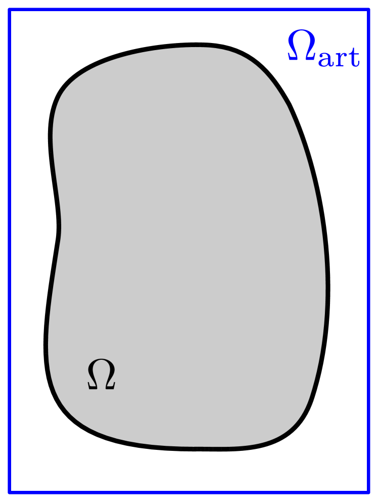
(a)

(b)

internal cells

cut cells

external cells

Figure 1. Embedded boundary setup.

We can also consider a partition of $\Omega$ into non-overlapping cell aggregates composed of cut cells and only one interior cell such that each aggregate is connected, using, e.g., the strategy described in Algorithm 4.1 below.

Algorithm 4.1 (Cell aggregation algorithm).

1. Mark all interior cells as touched and all cut cells as untouched.

2. For each untouched cell, if there is at least one touched cell connected to it through a facet $F$ such that $F\cap\Omega\neq\emptyset$, we aggregate the cell to the touched cell belonging to the aggregate containing the closest interior cell. If more than one touched cell fulfills this requirement, we choose one arbitrarily, e.g., the cell connected via the facet with more area inside the physical domain, or the one with smaller global label.

3. Mark as touched all the cells aggregated in step 2.

4. Repeat steps 2. and 3. until all cells are aggregated.

Fig. 2 shows an illustration of each step in Alg. 2. The black thin lines represent the boundaries of the aggregates. Note that from step 1 to step 2, some of the lines between adjacent cells are removed, meaning that the two adjacent cells have been merged in the same aggregate. The aggregation schemes can be easily applied to arbitrary spatial dimensions.

touched

untouched

Aggregates’ boundary

$\partial\Omega$

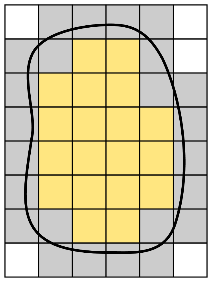
(a) Step 1.

(b) Step 2.

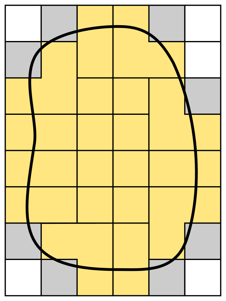
(c) Step 3.

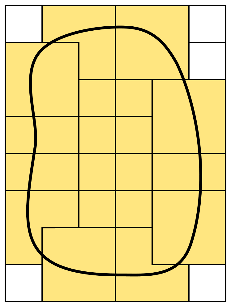
(d) Step 4.

Figure 2. Illustration of the cell aggregation scheme defined in Algorithm 4.1. We note that the definition of an aggregate in (5) is such that it only considers the part of the aggregated cells inside $\Omega$ as this simplifies the notation in the numerical analysis.

In the forthcoming sections, we need an upper bound of the size of the aggregates generated with Algorithm 4.1 in terms of the cell mesh size $h$, i.e., the characteristic size of an aggregate is bounded by $\gamma h$ for some $\gamma$ independent of $h$ and the cut cell intersection with the boundary. We refer to [8, Lem. 2.2] and the subsequent discusion for a bound of this quantity, supported with the numerical experiments in [8, Sect. 6.3].

Alg. 2 leads to another partition $\mathcal{T}_{h}$ into aggregates, where an aggregate is defined in terms of a set of cells as follows:

$$A\doteq\{\cup_{i=0}^{n_{A}}K_{i}\cap\Omega:\ K_{i}\in\mathcal{K}_{h}\},\qquad\forall A\in\mathcal{T}_{h},$$ (5)

where (without loss of generality) $K_{0}\in\mathcal{K}^{\rm in}_{h}$ is the owner interior cell, also represented with $\mathcal{O}(A)$. By construction of Algorithm 4.1, it holds: 1) $n_{A}\geq 0$; 2) interior cells that have no aggregated cut cells ($n_{A}=0$) remain the same; 3) there is only one interior cell per aggregate, i.e., $K_{i}\not\subset\Omega$ for $i>0$; 4) every cut cell belongs to one and only one aggregate.

For a interior/cut cell $K\in\mathcal{K}_{h}$, we define its owner (interior) cell $\mathcal{O}(K)$ as the owner $\mathcal{O}(A)$ of the only aggregate $A\in\mathcal{T}_{h}$ that contains the cell, i.e., $K\cup A$ has non-zero measure in dimension $d$. Thus, the owner of an interior cell is the cell itself.

We can also construct a map that, given an outer VEF, i.e., a VEF that belongs to at least one cut cell in $\mathcal{K}^{\rm cut}_{h}$ but does not belong to any interior cell in $\mathcal{K}^{\rm in}_{h}$, provides its aggregate owner among all the aggregates that contain it (see Fig. 3). This map can be arbitrarily built, e.g., we can consider the smallest aggregate that contain the VEF. The map between the outer VEF $b$ and the interior cell owner is also represented with $\mathcal{O}(b)$.

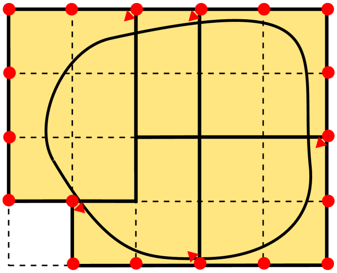
(a) Outer vertex to aggregate map

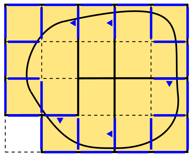
(b) Outer face to aggregate map

	Aggregate
	Cell
	Outer face
	Outer vertex

Figure 3. Map from outer faces and vertex to aggregate owner. The small pointers denote the aggregate owner. Pointers are not used for vertex and faces belonging to only one aggregate since the owner is obvious. Aggregates in (a) and (b) are the same, but the aggregate bounds are clearer in (a.

4.2. Aggregated finite element spaces

Our goal is to define FE spaces using the cell aggregates introduced above, in order to end up with unfitted FE spaces on the domain $\Omega$, with optimal approximability properties not affected by the small cut cell problem. In this work, the spaces will eventually be used for the interpolation of every velocity component and the pressure in the Stokes problem. Thus, it is enough to define the agFE spaces for a generic scalar-valued field.

Let us represent with ${\mathcal{V}_{h}}(\omega)$ a generic global and continuous Lagrangian FE space, i.e., it can be $\mathcal{Q}_{q,h}$ for hex meshes and $\mathcal{P}_{q,h}$ for tet meshes, for an arbitrary order $q$. We introduce the active FE space associated with the active portion of the background mesh ${\mathcal{V}_{h}^{\rm act}}\doteq{\mathcal{V}_{h}}(\mathcal{K}^{\rm act}_{h})$ and the interior FE space ${\mathcal{V}_{h}^{\rm in}}\doteq{\mathcal{V}_{h}}(\mathcal{K}^{\rm in}_{h})$. The active FE space ${\mathcal{V}_{h}^{\rm act}}$ (see Fig. 4(c)) is the functional space typically used in unfitted FE methods (see, e.g., [7, 5, 6]). It is well known that ${\mathcal{V}_{h}^{\rm act}}$ leads to arbitrary ill conditioned systems when integrating the FE weak form on the physical domain $\Omega$ only (if no stabilization technique is used to remedy it). It is obvious that the interior FE space ${\mathcal{V}_{h}^{\rm in}}$ (see Fig. 4(a)) is not affected by this problem, but it is not usable since it is not defined on $\Omega$.

Herein, we propose an alternative agFE space ${\mathcal{V}_{h}}$ that is defined on ${\Omega}$ but does not present the ill-conditioning issues related to ${\mathcal{V}_{h}^{\rm act}}$. To this end, we can define the set of nodes of ${\mathcal{V}_{h}^{\rm in}}$ and ${\mathcal{V}_{h}^{\rm act}}$ as $\mathcal{N}_{h}^{\rm in}$ and $\mathcal{N}_{h}^{\rm act}$, respectively (see Fig. 4). We define the set of outer nodes as $\mathcal{N}_{h}^{\rm out}\doteq\mathcal{N}_{h}^{\rm act}\setminus\mathcal{N}_{h}^{\rm in}$ (e.g., the nodes that belong to outer VEFs in Fig. 3). The outer nodes are the ones that can lead to conditioning problems due to the small cut cell problem (see, e.g., [5]). The space of global shape functions of ${\mathcal{V}_{h}^{\rm in}}$ and ${\mathcal{V}_{h}^{\rm act}}$ can be represented as $\{\phi^{b}\,:\,b\in\mathcal{N}_{h}^{\rm in}\}$ and $\{\phi^{b}\,:\,b\in\mathcal{N}_{h}^{\rm act}\}$, respectively. Any function $u_{h}\in{\mathcal{V}_{h}^{\rm in}}$ can be written as $u_{h}=\sum_{a\in\mathcal{N}_{h}^{\rm in}}u^{a}_{h}\phi^{a}$; analogously for functions in ${\mathcal{V}_{h}^{\rm act}}$. The space ${\mathcal{V}_{h}}$ is defined taking as starting point ${\mathcal{V}_{h}^{\rm act}}$, and adding judiciously defined constraints for the nodes in $\mathcal{N}_{h}^{\rm out}$.

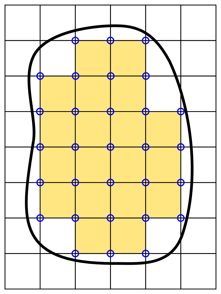
(a) ${\mathcal{V}_{h}^{\rm in}}$

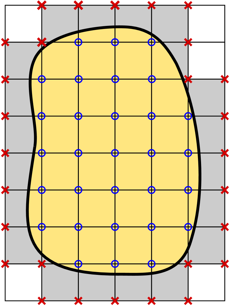
(b) ${\mathcal{V}_{h}}$

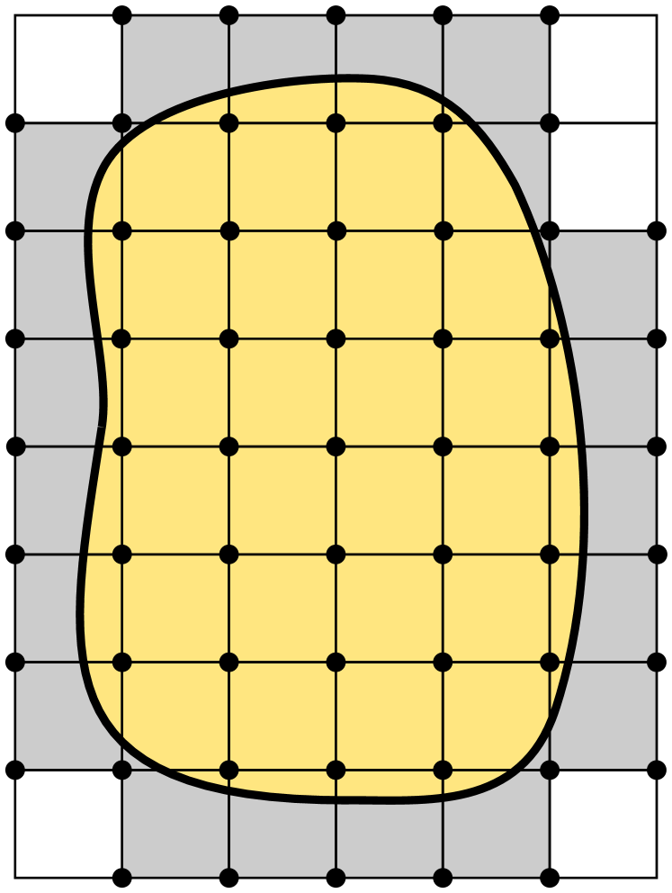
(c) ${\mathcal{V}_{h}^{\rm act}}$

$\circ$ nodes in $\mathcal{N}_{h}^{\rm in}$

$\bullet$ nodes in $\mathcal{N}_{h}^{\rm act}$

$\times$ nodes in $\mathcal{N}_{h}^{\rm out}$

Figure 4. Finite Element spaces.

In order to define ${\mathcal{V}_{h}}$, we observe that, in nodal Lagrangian FE spaces, there is a one-to-one map between DOFs and nodes (points) of the FE mesh. For globally continuous FE spaces, we can define the owner VEF of a node as the lowest-dimensional VEF that contains the node. As a result, the geometrical outer-VEF-to-cell-owner map above leads to an outer-DOF-to-cell-owner map too. Making abuse of notation, we also define the DOF map as $\mathcal{O}(b)$ for an outer DOF $b$.

Given a function $v_{h}\in{\mathcal{V}_{h}^{\rm in}}$ and a cell $K\in\mathcal{K}^{\rm in}_{h}$, we define the unique polynomial $\xi_{h}^{K}(v_{h}):\mathbb{R}^{d}\rightarrow\mathbb{R}$ such that its restriction to the cell $K$ coincides with the FE function, i.e., $v_{h}(\boldsymbol{x})=\xi_{h}^{K}(v_{h})(\boldsymbol{x})$, $\boldsymbol{x}\in K$. With these ingredients, we define ${\mathcal{V}_{h}}\subset{\mathcal{V}_{h}^{\rm act}}$ as the subset of functions in ${\mathcal{V}_{h}^{\rm act}}$ such that, for any DOF $a\in\mathcal{N}_{h}^{\rm out}$,

$$v_{h}^{a}=\sigma^{a}(\xi_{h}^{\mathcal{O}(a)}(v_{h}))=\sum_{b\in\mathcal{N}(\mathcal{O}(a))}\sigma^{a}(\xi_{h}^{\mathcal{O}(a)}(\phi^{b}))\sigma^{b}(v_{h}).$$ (6)

By construction, functions in ${\mathcal{V}_{h}}$ are uniquely determined by the DOFs of ${\mathcal{V}_{h}^{\rm in}}$. Thus, we can define the extension operator $\mathcal{E}:{\mathcal{V}_{h}^{\rm in}}\rightarrow{\mathcal{V}_{h}}\subset{\mathcal{V}_{h}^{\rm act}}$, such that, given $u_{h}\in{\mathcal{V}_{h}^{\rm in}}$ provides the FE function $\mathcal{E}_{h}(u_{h})\in{\mathcal{V}_{h}^{\rm act}}$ with outer nodal values computed as in (6). Thus, the agFE space is the range of this operator, i.e., ${\mathcal{V}_{h}}\doteq\mathcal{E}_{h}({\mathcal{V}_{h}^{\rm in}})\subset{\mathcal{V}_{h}^{\rm act}}$. Since ${\mathcal{V}_{h}}\subset{\mathcal{V}_{h}^{\rm act}}$, if ${\mathcal{V}_{h}^{\rm in}}$ and ${\mathcal{V}_{h}^{\rm act}}$ are $\mathcal{C}^{0}$ continuous, so it is ${\mathcal{V}_{h}}$. We note that (6) has sense for continuous and discontinuous spaces, and both tensor-product and serendipity spaces for hex meshes.

4.2.1. Nodal Lagrangian aggregated finite element spaces

In particular, for nodal-based Lagrangian FE spaces (which include tensor-product $\mathcal{Q}_{q,h}(\mathcal{K}_{h})$ and serendipity spaces $\breve{\mathcal{Q}}_{q,h}(\mathcal{K}_{h})$ for hex meshes and $\mathcal{P}_{q,h}(\mathcal{K}_{h})$ for tet meshes), the previous expression is reduced to:

$$v_{h}(\boldsymbol{x}^{a})=\sum_{b\in\mathcal{N}(\mathcal{O}(a))}v_{h}(\boldsymbol{x}^{b})\phi^{b}(\boldsymbol{x}^{a}).$$ (7)

The computation of the constraint is straightforward, and simply involves to evaluate the shape function polynomials of a cell in a set of points that do not belong to the cell, viz., the nodes of an aggregated cut cell. The definition of DOF ownership is simple, the VEF or cell that contains the node related to the DOF with minimum dimension, which is uniquely defined.

4.2.2. Discontinuous aggregated finite element spaces

Let us comment on discontinuous FE spaces, e.g., $\mathcal{P}^{-}_{q,h}(\mathcal{K}_{h})$ on hex meshes. In this case, all the DOFs belong to the cell itself, since no continuity must be enforced. Thus, the DOFs owner and DOFs-to-cell maps are trivial once defined the cell aggregation. Since no continuity must be enforced among cells, the DOFs definition is very flexible. The definition in (6) is general and can be used for discontinuous spaces with DOFs that are not nodal evaluations. It is easy to check that for discontinuous spaces, the agFE space can be analogously defined as:

$${\mathcal{V}_{h}}=\{v:\,v|_{A}\in\mathcal{P}_{q}^{-}(A),\,\hbox{for any}\ A\in\mathcal{T}_{h}\}.$$ (8)

The equivalence between the definition based on (6) and the one in (8) is straightforward. The use of aggregation techniques within DG methods has already been used, e.g., in [28, 17].

4.2.3. Aggregated finite elements with serendipity extension

Up to now, we have assumed that the constraints for the extension operator were computed using the same shape functions as the ones of the local FE space in the owner interior cell (see (6)). Here, we consider a more general case in which these two shape functions bases (and the corresponding spanned spaces) can differ. In particular, we are interested in using a tensor-product Lagrangian space at all cells in a hex mesh, but to compute the constraints through the corresponding serendipity basis (preserving the order of approximation). As we will see later on, it does not affect accuracy and has positive properties when considering stable mixed agFE spaces.

Let us introduce some notation, in order to distinguish between tensor-product and serendipity FE spaces. For serendipity FEs and hex meshes, i.e., $\breve{\mathcal{Q}}_{q}(K)$, we represent its unisolvent set of nodes with $\breve{\mathcal{N}}(K)$, i.e., the corresponding nodal values are a basis for the dual space, with cardinality $\breve{n}_{\Sigma}$ (see [25, Fig. 1]). The corresponding shape functions and DOFs are represented with $\{\breve{\phi}^{a}\}_{a\in\breve{\mathcal{N}}(K)}$ and $\{\breve{\sigma}^{a}\}_{a\in\breve{\mathcal{N}}(K)}$, respectively. For serendipity spaces, we denote its corresponding nodal interpolator in (4) as $\breve{\pi}^{I}_{K}(v)$.

We constrain every outer DOF $a\in\mathcal{N}_{h}^{\rm out}$ of a function $v_{h}\in{\mathcal{V}_{h}^{\rm act}}$ as

$$v_{h}^{a}=\sigma^{a}(\xi_{h}^{\mathcal{O}(a)}\circ\breve{\pi}^{I}_{\mathcal{O}(a)}(v_{h})))=\sum_{b\in\breve{\mathcal{N}}(\mathcal{O}(a))}\sigma^{a}(\xi_{h}^{\mathcal{O}(a)}(\breve{\phi}^{b}))\breve{\sigma}^{b}(v_{h}),$$ (9)

or analogously,

$$v_{h}(\boldsymbol{x}^{a})=\sum_{b\in\breve{\mathcal{N}}(\mathcal{O}(a))}v_{h}(\boldsymbol{x}^{b})\breve{\phi}^{b}(\boldsymbol{x}^{a}).$$ (10)

It leads to the new agFE space ${\breve{\mathcal{V}}_{h}}$ and its corresponding extension operator $\breve{\mathcal{E}}_{h}$.

4.3. Mathematical properties

In the following, we list some FE inequalities that will be used in the next sections. We use $A\lesssim B$ to say that $A<CB$ for some positive constant $C$; analogously for $\gtrsim$ and $\eqsim$. We use $C$ to denote such a constant, which can be different in different appearances. The word constant in this work always denotes independence with respect to $h$ and the cut cell intersection, i.e., it is not affected by the small cut cell problem.

Let us consider an arbitrary FE space ${\mathcal{V}_{h}}$. The following inverse inequalities hold (see, e.g., [27]):

$${\|{\boldsymbol{\nabla}}u_{h}\|}_{{K}} \lesssim h_{K}^{-1}{\|u_{h}\|}_{{K}},$$ (11)

$${\|{\partial_{\boldsymbol{n}}}u_{h}\|}_{{{\Gamma}\cap K}} \lesssim h_{K}^{-\frac{1}{2}}{\|{\boldsymbol{\nabla}}u_{h}\|}_{{{K}}},$$ (12)

where ${\boldsymbol{n}}$ is the outward normal (in this appearance, with respect to ${\Gamma}_{\rm D}\cap K$), and ${\partial_{\boldsymbol{n}}}\doteq{\boldsymbol{n}}\cdot{\boldsymbol{\nabla}}$. Furthermore, we have the following trace inequalities (see [29]):

$${\|u_{h}\|}_{{\partial K}} \lesssim h_{K}^{-\frac{1}{2}}{\|u_{h}\|}_{{K}}+h_{K}^{\frac{1}{2}}{\|{\boldsymbol{\nabla}}u_{h}\|}_{{K}}.$$ (13)

$${\|u_{h}\|}_{{{\Gamma}\cap K}} \lesssim h_{K}^{-\frac{1}{2}}{\|u_{h}\|}_{{K}}+h_{K}^{\frac{1}{2}}{\|{\boldsymbol{\nabla}}u_{h}\|}_{{K}},$$ (14)

(We note that (14) implies (13)). The extension operators $\mathcal{E}_{h}(\cdot)$ and $\breve{\mathcal{E}}_{h}(\cdot)$ satisfy the following stability bounds. The standard extension operator can be considered for both tet and hex meshes, whereas the serendipity extension operator only for hex meshes.

Lemma 4.2.

Given a function $u_{h}\in{\mathcal{V}_{h}^{\rm in}}$, it holds:

$${\|\mathcal{E}_{h}(u_{h})\|}_{{{\Omega_{\rm act}}}}\lesssim{\|u_{h}\|}_{{{\Omega_{\rm in}}}},\quad {\|{\breve{\mathcal{E}}_{h}(u_{h})}\|}_{{{\Omega_{\rm act}}}}\lesssim{\|u_{h}\|}_{{{\Omega_{\rm in}}}},$$ (15)

$${\|{\boldsymbol{\nabla}}\mathcal{E}_{h}(u_{h})\|}_{{{\Omega_{\rm act}}}}\lesssim{\|{\boldsymbol{\nabla}}u_{h}\|}_{{{\Omega_{\rm in}}}},\quad {\|{\boldsymbol{\nabla}}\breve{\mathcal{E}}_{h}(u_{h})\|}_{{{\Omega_{\rm act}}}}\lesssim{\|{\boldsymbol{\nabla}}u_{h}\|}_{{{\Omega_{\rm in}}}}.$$ (16)

Proof.

The proof for $\mathcal{E}_{h}(\cdot)$ can be found in [8, Corollary 5.3] for a general agFE space, that can be either ${\mathcal{V}_{h}^{\rm in}}$ or the discontinuous FE space of its gradients. The results for $\breve{\mathcal{E}}_{h}(\cdot)$ can be proved analogously. ∎

Given the interior FE space ${\mathcal{V}_{h}^{\rm in}}$, we can define the standard Scott-Zhang interpolation using the standard definition in [30]. Let us define an extended Scott-Zhang interpolant as follows: 1) perform the standard interior Scott-Zhang interpolator onto ${\mathcal{V}_{h}^{\rm in}}$ through the assignment for every interior DOF $a\in\mathcal{N}_{h}^{\rm in}$ of an arbitrary VEF/cell $\tilde{K}_{a}\subset{\Omega_{\rm in}}$ that contains the owner VEF of $a$, and compute the mean value of the function on $\tilde{K}_{a}$, represented with $\sigma^{SZ,a}_{\tilde{K}_{a}}(\cdot)$; 2) extend the interior function to $\Omega$ using the extension operator $\mathcal{E}_{h}(\cdot)$ (or $\breve{\mathcal{E}}_{h}(\cdot)$), leading to a function in ${\mathcal{V}_{h}}$ (or ${\breve{\mathcal{V}}_{h}}$). Thus, the extended Scott-Zhang interpolant reads:

$$\pi_{h}^{SZ}(u)(\boldsymbol{x})\doteq\sum_{a\in\mathcal{N}_{h}^{\rm in}}\sigma^{SZ,a}_{\tilde{K}_{a}}(u)\mathcal{E}(\phi^{a}(\boldsymbol{x})).$$

The serendipity-extended interpolant, represented with $\breve{\pi}_{h}^{SZ}(u)$, is obtained as above, but using $\breve{\mathcal{E}}_{h}(\cdot)$ instead.

In the next theorem, we prove the approximability properties of the extended Scott-Zhang interpolant. In the statement of the theorem, we represent with $\omega(A)$ the union of the owner of the aggregate itself and the owners of all its neighbors, i.e., $\omega(A)\doteq\{\mathcal{O}(B):A\cap B\neq\emptyset,\ B\in\mathcal{T}_{h}\}$. We note that $A\not\subseteq\omega(A)\subset{\Omega_{\rm in}}$ in general.

Theorem 4.3.

Let us consider an agFE space ${\mathcal{V}_{h}}$ such that $\mathcal{P}_{q}(A)\subset{\mathcal{V}_{h}}(A)$ for $A\in\mathcal{T}_{h}$, $q\in\mathbb{N}^{+}$. Let us consider a function $u\in W_{p}^{m}(\Omega)$, where $1\leq p\leq\infty$, $m\leq q+1$, and $m\geq d$ for $p=1$ or $m>\frac{d}{p}$ for $p>1$. It holds:

$$\|u-\pi_{h}^{SZ}(u)\|_{W_{p}^{s}(A)}\lesssim{h}^{m-s}|u|_{W_{p}^{m}(\omega(A))},\qquad \|u-\pi_{h}^{SZ}(u)\|_{W_{p}^{s}(S)}\lesssim{h}^{m-s-\frac{1}{2}}|u|_{W_{p}^{m}(\omega(A))},$$ (17)

for $1\leq s\leq m$, $A\in\mathcal{T}_{h}$, and $S$ being the intersection between a plane in $\mathbb{R}^{d}$ and $A$. The same results apply for the serendipity-extended agFE space ${\breve{\mathcal{V}}_{h}}$ and its corresponding interpolant $\breve{\pi}_{h}^{SZ}(\cdot)$.

Proof.

The standard and serendipity interpolants can be analyzed analogously. The Scott-Zhang moments $\sigma^{SZ,a}_{\tilde{K}_{a}}(\cdot)$ are bounded in $W^{m}_{p}(\Omega)$ owing to the trace theorem, i.e., $W_{p}^{l}(\Omega)\subset L^{1}(\tilde{K}_{a})$ for $\tilde{K}_{a}$ being a facet or cell (see [30]). On the other hand, $\mathcal{E}(\phi^{a}(\boldsymbol{x}))\in W_{\infty}^{m}(\Omega)\subset W_{p}^{m}(\Omega)$, since it is a combination of shape function with bounded nodal values (see (6) and Lem. 4.2). Moreover, from the definition of the extension operator, the nodal values of $\pi_{h}^{SZ}(\cdot)|_{A}$ are constrained from the DOFs of the owner interior cell of $A$ or the DOFs of the owner cell of a neighbor of $A$. Thus, we readily obtain that $\|\pi_{h}^{SZ}(u)\|_{W_{p}^{m}(A)}\leq C\|u\|_{W_{p}^{m}(\omega(A))}$. Next, we consider an arbitrary function $\pi(u)\in W_{p}^{m}(\Omega)$ such that $\pi(u)|_{K}\in\mathcal{P}_{q}(\omega(A))\subset{\mathcal{V}_{h}}(\omega(A))$ (note that the inclusion also holds for the serendipity extension). The fact that $\pi_{h}^{SZ}(\cdot)$ is a projection onto ${\mathcal{V}_{h}}$ by construction yields $\pi(u)|_{A}=\pi_{h}^{SZ}(\pi(u))|_{A}$. Thus, we have:

$$\|u-\pi_{h}^{SZ}(u)\|_{W_{p}^{m}(A)} \leq\|u-\pi(u)\|_{W_{p}^{m}(A)}+\|\pi_{h}^{SZ}(\pi(u)-u)\|_{W_{p}^{m}(A)}$$ (18)

$$\lesssim\|u-\pi(u)\|_{W_{p}^{m}(A)}+\|\pi(u)-{u}\|_{W_{p}^{m}(\omega(A))}\lesssim\|u-\pi(u)\|_{W_{p}^{m}(\omega(A))}.$$ (19)

Since $\omega(A)$ is an open bounded domain with Lipschitz boundary by definition, one can use the Deny-Lions lemma (see, e.g., [31]). As a result, using the $\pi(u)$ that minimizes the right-hand side, it holds:

$$\|u-\pi_{h}^{SZ}(u)\|_{W_{p}^{m}(A)}\lesssim|u|_{W_{p}^{m}(\omega(A))}.$$ (20)

The Sobolev embedding theorem and the trace theorem yield:

$$\|u-\pi_{h}^{SZ}(u)\|_{W_{p}^{s}(A)}\leq C(A)|u|_{W_{p}^{m}(\omega(A))},\qquad$$ (21)

$$\|u-\pi_{h}^{SZ}(u)\|_{W_{p}^{s-\frac{1}{2}}(S)}\leq\|u-\pi_{h}^{SZ}(u)\|_{W_{p}^{s}(A)}\leq C(A)|u|_{W_{p}^{m}(\omega(A))}.$$ (22)

Using standard scaling arguments, we prove the lemma. ∎

5. Approximation of the Stokes problem

In this section, we consider the FE approximation of the Stokes problem (1) using agFE spaces on unfitted meshes. We focus on extended by aggregation inf-sup stable spaces (velocity-pressure pairs of FE spaces that satisfy a discrete version of the inf-sup condition on body-fitted meshes) with additional stabilizing terms to cure the potential deficiencies of the unfitted inf-sup condition. In this section, the velocity and pressure spaces are represented with $\boldsymbol{V}_{h}$ and $Q_{h}$, respectively. As usual in unfitted FE methods, the Dirichlet boundary conditions cannot be enforced strongly. Instead, we consider a Nitsche-type weak imposition of the Dirichlet data [32, 33]. It provides a consistent numerical scheme with optimal converge rates (also for high-order elements) that is commonly used in the embedded boundary community (see, e.g., [22] for its application in unfitted discretizations of the Stokes problem). Another important ingredient in unfitted FE approximations is the integration on cut cells. We refer to [7] for a detailed exposition of the particular technique used in this paper. With these ingredients, we define the Stokes operator:

$$A_{h}(\boldsymbol{u}_{h},p_{h},\boldsymbol{v}_{h},q_{h})\doteq a_{h}(\boldsymbol{u}_{h},\boldsymbol{v}_{h})+b_{h}(\boldsymbol{v}_{h},p_{h})+b_{h}(\boldsymbol{u}_{h},q_{h})-j_{h}(\boldsymbol{u}_{h},p_{h},\boldsymbol{v}_{h},q_{h}),$$ (23)

where

$$a_{h}(\boldsymbol{u}_{h},\boldsymbol{v}_{h}) \doteq\left({\boldsymbol{\nabla}}\boldsymbol{u}_{h},{\boldsymbol{\nabla}}\boldsymbol{v}_{h}\right)_{\Omega}-\left({\partial_{\boldsymbol{n}}}\boldsymbol{u}_{h},\boldsymbol{v}_{h}\right)_{{\Gamma}}-\left({\partial_{\boldsymbol{n}}}\boldsymbol{v}_{h},\boldsymbol{u}_{h}\right)_{{\Gamma}}+{\tau}\left({h}\boldsymbol{u}_{h},\boldsymbol{v}_{h}\right)_{{\Gamma}},$$ (24)

$$b_{h}(\boldsymbol{v}_{h},p_{h}) \doteq-\left({\boldsymbol{\nabla}}\cdot\boldsymbol{v}_{h},p_{h}\right)_{\Omega}+\left({\boldsymbol{n}}\cdot\boldsymbol{v}_{h},p_{h}\right)_{{\Gamma}},$$ (25)

with ${\tau}$ a large enough positive constant, for stability purposes. The right-hand side reads:

$$L_{h}(\boldsymbol{v}_{h},q_{h})\doteq\left({\boldsymbol{f}},\boldsymbol{v}_{h}\right)_{\Omega}+g_{h}({\boldsymbol{f}},\boldsymbol{v}_{h}).$$ (26)

The pressure stabilization term $j_{h}$ and the corresponding potential modification of the right-hand side $g_{h}$ to keep consistency will be defined in Sect. 6.2, motivated from the numerical analysis. The discrete Stokes problem finally reads: find $(\boldsymbol{u}_{h},\,p_{h})\in\boldsymbol{V}_{h}\times Q_{h}$ such that

$$A_{h}(\boldsymbol{u}_{h},p_{h},\boldsymbol{v}_{h},q_{h})=L_{h}(\boldsymbol{v}_{h},p_{h}),\qquad\forall\,(\boldsymbol{v}_{h},\,q_{h})\in\boldsymbol{V}_{h}\times Q_{h}.$$ (27)

In the following analysis, we restrict ourselves to hexahedral meshes and discontinuous pressures. Similar ideas can be applied to inf-sup stable mixed FEs on tetrahedral meshes and continuous pressures, but we do not consider these cases for the sake of conciseness. Thus, using the notation in Sect. 4.2, we will make use of the following global agFE spaces: the space $\mathcal{Q}_{q,h}$, for $q\geq 1$, in which the local FE space is the tensor-product Lagrangian $\mathcal{Q}_{q}(K)$ in all cells $K\in\mathcal{K}_{h}$, and the constraints are defined using the standard expression in (7); the space $\breve{\mathcal{Q}}_{q,h}$, for $q\geq 1$, which only differs from the previous one in the constraint definition, based now on the serendipity extension in (10); the discontinuous space $\mathcal{P}^{-}_{q,h}$, for $q\geq 0$, defined in (8).

6. Numerical analysis

In this section, we perform the stability analysis of FE methods for (23). First, in Sect. 6.1, we consider an abstract stability analysis , i.e., we prove an inf-sup condition under some assumptions over the mixed agFE space and the stabilization terms. Two different algorithms that satisfy these assumptions, and thus are stable, are proposed in Sect. 6.2. A priori error estimates for these methods are obtained in Sect. 6.3. Finally, in Sect. 6.4, we prove condition number bounds that are independent of the cut cell intersection with the boundary, i.e., the small cut cell problem.

The analysis of the discrete problem obviously relies on the well-posedness of the continuous problem, i.e., the inf-sup condition in (3). For the sake of conciseness in notation, we have not distinguished between the actual computational domain $\Omega_{h}$ and the physical domain $\Omega$. However, it is important to distinguish between these two in the definition of the inf-sup constant, i.e., $\beta(\Omega)$ vs. $\beta(\Omega_{h})$. In general, $\beta(\Omega_{h})$ can tend to zero as $h\to 0$. The lower bound for $\beta(\cdot)$ relies on a decomposition of the domain into a finite number of strictly star shaped domains. $\beta(\Omega_{h})$ could tend to zero as $h\to 0$ unless one can prove that this number is bounded away from zero for $\Omega_{h}$. It is in fact a problem for methods that rely on inf-sup conditions for ${\Omega_{\rm in}}$ (see [21]). Even though it is hard to imagine that a reasonable smooth approximation $\Omega_{h}$ of $\Omega$ would require a decomposition into a number of star shaped domains that blows up as $h\to 0$, there are constructions of $\Omega_{h}$ for which one can prove that in fact $\beta(\Omega_{h})$ is bounded below, or even more, converges to $\beta(\Omega)$. In particular, if $\Omega_{h}$ is a polygonal $h$-approximation of $\Omega$ in the sense of [34, Def. 4.5], it holds $|\beta(\Omega)-\beta(\Omega_{h})|\leq c(\Omega)h$. In what follows, we simply consider $\beta\doteq\inf_{h<h_{0}}\beta(\Omega_{h})$, for $h_{0}$ a fine enough mesh size to represent the topology of the geometry at hand.

6.1. An abstract stability analysis

In this section, we analyze the well-posedness of the discretization of the Stokes problem (23) in an abstract setting, in which the FE spaces and stabilization terms are not explicitly stated. Instead, we do the analysis under some assumptions of these ingredients.

We define the following norms:

$$\mathopen{|\mkern-1.5mu|\mkern-1.5mu|}\boldsymbol{u}\mathclose{|\mkern-1.5mu|\mkern-1.5mu|}_{h}^{2}\doteq{\|{\boldsymbol{\nabla}}\boldsymbol{u}\|}_{{\Omega}}^{2}+{\|h^{-\frac{1}{2}}\boldsymbol{u}\|}_{{{\Gamma}}}^{2},\qquad\mathopen{|\mkern-1.5mu|\mkern-1.5mu|}\boldsymbol{u},\,p\mathclose{|\mkern-1.5mu|\mkern-1.5mu|}_{h}^{2}\doteq\mathopen{|\mkern-1.5mu|\mkern-1.5mu|}\boldsymbol{u}\mathclose{|\mkern-1.5mu|\mkern-1.5mu|}_{h}^{2}+{\|p\|}_{{\Omega}}^{2}.$$ (28)

In the following lemma, we prove some stability and continuity properties of the different terms that compose the Stokes operator in (23).

Lemma 6.1.

It holds for any $\boldsymbol{u}_{h},\,\boldsymbol{v}_{h}\in\boldsymbol{V}_{h}$

$$a_{h}(\boldsymbol{u}_{h},\boldsymbol{u}_{h})\geq\gamma_{a}\mathopen{|\mkern-1.5mu|\mkern-1.5mu|}\boldsymbol{u}_{h}\mathclose{|\mkern-1.5mu|\mkern-1.5mu|}_{h}^{2},\qquad a_{h}(\boldsymbol{u}_{h},\boldsymbol{v}_{h})\leq\xi_{a}\mathopen{|\mkern-1.5mu|\mkern-1.5mu|}\boldsymbol{u}_{h}\mathclose{|\mkern-1.5mu|\mkern-1.5mu|}_{h}\mathopen{|\mkern-1.5mu|\mkern-1.5mu|}\boldsymbol{v}_{h}\mathclose{|\mkern-1.5mu|\mkern-1.5mu|}_{h},\qquad b_{h}(\boldsymbol{v}_{h},q_{h})\leq\xi_{b}\mathopen{|\mkern-1.5mu|\mkern-1.5mu|}\boldsymbol{v}_{h}\mathclose{|\mkern-1.5mu|\mkern-1.5mu|}_{h}\mathopen{|\mkern-1.5mu|\mkern-1.5mu|}q_{h}\mathclose{|\mkern-1.5mu|\mkern-1.5mu|}_{h}.$$ (29)

for ${\tau}$ a large enough positive constant in (24).

Proof.

The continuity and stability of $a_{h}$ can be found, e.g., in [8, Th. 5.7]. The continuity of $b_{h}$ is obtained by using in its two terms the Cauchy-Schwarz inequality and in the second one the inequalities (11) and (14) (see also [22]). ∎

Next, we prove the unfitted inf-sup condition for agFE spaces, using the following strategy. First, we introduce some definitions for the concept of improper facets and aggregates (Defs. 6.2-6.3 and 6.4-6.5) which are the ones that will require some type of stabilization, due to the potential deficiency of the discrete inf-sup condition. Second, we prove a weak inf-sup condition for a particular type of mixed FE spaces in Th. 6.9. Finally, using an abstract definition of the pressure stabilization term that satisfies Asm. 6.10, we prove the stability of the agFE method for the Stokes problem in Th. 6.11. In the subsequent sections, we will consider different realizations of mixed FE spaces, analyze how to determine a superset of improper facets/aggregates, and define a pressure stabilization fulfilling Asm. 6.10 for (23) to be well-posed.

Let us define the set of aggregate interfaces:

$$\qquad F_{AB}\doteq\partial A\cap\partial B,\ \ A,\,B\in\mathcal{T}_{h},\qquad\mathcal{F}_{h}\doteq\{F_{AB}\,:\,A,\,B\in\mathcal{T}_{h}\}.$$

We note that, since $A\subset\Omega$ for any aggregate $A\in\mathcal{T}_{h}$ by its definition in (5), $F_{AB}$ can include a cut facet of a cut cell.

Definition 6.2 (Aggregate interface bubble).

Given an aggregate interface $F_{AB}\in\mathcal{F}_{h}$ shared by $A,\,B\in\mathcal{T}_{h}$, an aggregate interface bubble is a function $\boldsymbol{\phi}_{h}^{F_{AB}}\in\boldsymbol{V}_{h}$ with $\sup(\boldsymbol{\phi}_{h}^{F_{AB}})\subseteq AB\doteq A\cup B$ such that

$$\int_{F_{AB}}\boldsymbol{\phi}_{h}^{F_{AB}}\cdot{\boldsymbol{n}}>C|F_{AB}|>0,\quad\|\boldsymbol{\phi}_{h}^{F_{AB}}\|_{\infty}\leq C,\quad\boldsymbol{\phi}_{h}^{F_{AB}}\cdot{\boldsymbol{n}}={0}\ \ \hbox{on}\ \ \partial AB.$$

Definition 6.3 (Improper interface set of $\boldsymbol{V}_{h}$).

Given an aggregate interface $F_{AB}$ shared by $A,\,B\in\mathcal{T}_{h}$, it is improper with respect to $\boldsymbol{V}_{h}$ if there not exists any interface bubble satisfying the properties of Def. 6.2. The set of improper interfaces is denoted by $\mathcal{F}_{h}^{-}$. Its complement is represented with $\mathcal{F}_{h}^{+}\doteq\mathcal{F}_{h}\setminus\mathcal{F}_{h}^{-}$.

Definition 6.4 (Aggregate bubble).

Given an aggregate $A\in\mathcal{T}_{h}$, an aggregate bubble is a function ${\phi}^{A}_{h}\in\boldsymbol{\mathcal{Q}}_{2}(A)\cap H_{0}^{1}(A)$ with $\sup({\phi}^{A}_{h})\subseteq A$ such that:

$$\boldsymbol{\phi}_{h}^{A}(\boldsymbol{x})\geq 0,\quad\int_{A}\boldsymbol{\phi}_{h}^{A}>C|A|>0,\quad\|\boldsymbol{\phi}_{h}^{A}\|_{\infty}\leq C.$$ (30)

Definition 6.5 (Improper aggregate set of $\boldsymbol{V}_{h}$).

Given an aggregate $A\in\mathcal{T}_{h}$, it is improper with respect to $\boldsymbol{V}_{h}$ if there not exists any aggregate bubble satisfying the properties of Def. 6.4. The set of improper aggregates is denoted by $\mathcal{T}_{h}^{-}$. Its complement is represented with $\mathcal{T}_{h}^{+}\doteq\mathcal{T}_{h}\setminus\mathcal{T}_{h}^{-}$.

In the next lemma we propose a weak version of the standard Fortin interpolator (see, e.g., [31]), which we denote as quasi-Fortin interpolator.

Lemma 6.6 (Quasi-Fortin interpolant).

For any $\boldsymbol{v}\in\boldsymbol{H}^{1}_{\boldsymbol{0}}(\Omega)$, there exists a function $\pi^{qF}_{h}(\boldsymbol{v})\in\boldsymbol{V}_{h}$ such that:

$$\int_{F}\boldsymbol{v}\cdot{\boldsymbol{n}}=\int_{F}\pi_{h}^{qF}(\boldsymbol{v})\cdot{\boldsymbol{n}}\quad\forall F\in\mathcal{F}_{h}^{+},\qquad\mathopen{|\mkern-1.5mu|\mkern-1.5mu|}\pi_{h}^{qF}(\boldsymbol{v})\mathclose{|\mkern-1.5mu|\mkern-1.5mu|}_{h}\leq\xi_{qF}{\|\boldsymbol{v}\|}_{1,\Omega},$$ (31)

for a positive constant $\xi_{qF}>0$.

Proof.

Given a function $\boldsymbol{v}\in\boldsymbol{H}^{1}_{\boldsymbol{0}}(\Omega)$, let us consider, e.g., the extended Scott-Zhang interpolant $\pi_{h}^{SZ}(\boldsymbol{v}_{h})$ with the optimal approximability properties in Th. 4.3. For agFE spaces with serendity extensions, we would consider $\breve{\pi}_{h}^{SZ}(\boldsymbol{v}_{h})$ instead. From Def. 6.2, at every proper interface $F\in\mathcal{F}_{h}^{+}$, we can compute $\zeta_{F}(\boldsymbol{v})\in\mathbb{R}$ such that:

$$\zeta_{F}(\boldsymbol{v})\int_{F}\boldsymbol{\phi}_{h}^{F}\cdot{\boldsymbol{n}}=\int_{F}(\boldsymbol{v}-\pi_{h}^{SZ}(\boldsymbol{v}))\cdot{\boldsymbol{n}},$$ (32)

and define $\boldsymbol{\zeta}_{h}(\boldsymbol{v})=\sum_{F\in\mathcal{F}_{h}^{+}}\boldsymbol{\phi}_{h}^{F}\zeta_{F}(\boldsymbol{v})$. Thus, taking $\pi_{h}^{qF}(\boldsymbol{v})\doteq\pi_{h}^{SZ}(\boldsymbol{v})+\boldsymbol{\zeta}_{h}(\boldsymbol{v})$, one readily checks the equality in (31). Next, we prove the stability of the quasi-Fortin interpolant. We can bound $\zeta_{F}(\boldsymbol{v})$, since $F\in\mathcal{F}_{h}^{+}$, as follows. Let us represent with $A_{F}\in\mathcal{T}_{h}$ one of the two aggregates sharing $F$. The definition of the aggregate bubble in Def. 6.4, the extended Scott-Zhang approximability properties in (17), the inverse inequality (14), and the Cauchy-Schwarz inequality yield:

$$\zeta_{F} =\frac{\int_{F}(\boldsymbol{v}-\pi_{h}^{SZ}(\boldsymbol{v}))\cdot{\boldsymbol{n}}}{\int_{F}\boldsymbol{\phi}_{h}^{F}\cdot{\boldsymbol{n}}}\lesssim\frac{\int_{F}(\boldsymbol{v}-\pi_{h}^{SZ}(\boldsymbol{v}))\cdot{\boldsymbol{n}}}{|F|}\lesssim\frac{{\|\boldsymbol{v}-\pi_{h}^{SZ}(\boldsymbol{v})\|}_{{F}}}{|F|^{\frac{1}{2}}}$$ (33)

$$\lesssim h^{-\frac{d-1}{2}}{\|\boldsymbol{v}-\pi_{h}^{SZ}(\boldsymbol{v})\|}_{{\partial A_{F}}}\lesssim h^{-\frac{d-1}{2}}(h^{-\frac{1}{2}}{\|\boldsymbol{v}-\pi_{h}(\boldsymbol{v})\|}_{{A_{F}}}+h^{\frac{1}{2}}{|\boldsymbol{v}-\pi_{h}(\boldsymbol{v})|}_{1,A_{F}})\lesssim h^{-\frac{d-2}{2}}{\|\boldsymbol{v}\|}_{1,\omega(A_{F})}.$$

Using scaling arguments and the properties of the interface bubbles in Def. 6.2 and (33), and the fact that for any interior cell $K\in\mathcal{K}^{\rm in}_{h}$, the cardinality of the set $\{A\in\mathcal{T}_{h}\ :\ K\subseteq\omega(A)\}$ is bounded independently of $h$, we get:

$$\mathopen{|\mkern-1.5mu|\mkern-1.5mu|}\boldsymbol{\zeta}_{h}(\boldsymbol{v})\mathclose{|\mkern-1.5mu|\mkern-1.5mu|}_{h}^{2}=\sum_{F\in\mathcal{F}_{h}^{+}}{\|\zeta_{F}\boldsymbol{\phi}_{h}^{F}\|}_{1,AB_{F}}^{2}\lesssim\sum_{F\in\mathcal{F}_{h}^{+}}\zeta_{F}^{2}h^{d-2}\|\boldsymbol{\phi}_{h}^{F}\|^{2}_{L^{\infty}(AB_{F})}\lesssim\sum_{F\in\mathcal{F}_{h}^{+}}{\|\boldsymbol{v}\|}_{1,\omega(A_{F})}^{2}\lesssim{\|\boldsymbol{v}\|}_{1,\Omega}^{2}.$$ (34)

This result, combined with the stability and approximability of the Scott-Zhang projector and the triangle inequality, leads to the stability of the quasi-Fortin interpolant in (31):

$$\mathopen{|\mkern-1.5mu|\mkern-1.5mu|}\pi_{h}^{qF}(\boldsymbol{v})+\boldsymbol{\zeta}_{h}(\boldsymbol{v})\mathclose{|\mkern-1.5mu|\mkern-1.5mu|}_{h}\lesssim\mathopen{|\mkern-1.5mu|\mkern-1.5mu|}\pi_{h}^{qF}(\boldsymbol{v})\mathclose{|\mkern-1.5mu|\mkern-1.5mu|}_{h}+\mathopen{|\mkern-1.5mu|\mkern-1.5mu|}\boldsymbol{\zeta}_{h}(\boldsymbol{v})\mathclose{|\mkern-1.5mu|\mkern-1.5mu|}_{h}\lesssim{\|\boldsymbol{v}\|}_{1,\Omega}.$$ (35)

It proves the lemma. ∎

Lemma 6.7.

Given an aggregate $A\in\mathcal{T}_{h}^{+}$, we consider the aggregate bubble function ${\phi}^{A}_{h}\in H^{1}_{{0}}(A)$ that satisfies the properties in Def. 6.5. For any $p_{h}\in Q_{h}$, the function $\boldsymbol{\varphi}_{h}(p_{h})\doteq\sum_{A\in\mathcal{T}_{h}^{+}}{\phi}^{A}_{h}{h}^{2}{\boldsymbol{\nabla}}p_{h}$ satisfies the following properties:

$$\frac{1}{\beta_{0}^{\prime}}\sum_{A\in\mathcal{T}_{h}^{+}}{\|p_{h}-\pi_{h}^{-,0}(p_{h})\|}_{{A}}^{2}\leq b_{h}(\boldsymbol{\varphi}_{h}(p_{h}),p_{h}),\qquad\mathopen{|\mkern-1.5mu|\mkern-1.5mu|}\boldsymbol{\varphi}_{h}(p_{h})\mathclose{|\mkern-1.5mu|\mkern-1.5mu|}_{h}^{2}\leq\sum_{A\in\mathcal{T}_{h}^{+}}{\|p_{h}-\pi_{h}^{-,0}(p_{h})\|}_{{A}}^{2}.$$ (36)

Proof.

The fact that $\boldsymbol{\varphi}_{h}(p_{h})$ vanishes on ${\Gamma}$, the definition of the norms in (28), and the inverse inequality (11), yield the continuity bound in (36):

$$\mathopen{|\mkern-1.5mu|\mkern-1.5mu|}\boldsymbol{\varphi}_{h}(p_{h})\mathclose{|\mkern-1.5mu|\mkern-1.5mu|}_{h}^{2}={\|\boldsymbol{\varphi}_{h}(p_{h})\|}_{1,\Omega}^{2}\lesssim\sum_{A\in\mathcal{T}_{h}^{+}}h^{2}\|{\boldsymbol{\nabla}}p_{h}\|^{2}=\sum_{A\in\mathcal{T}_{h}^{+}}h^{2}\|{\boldsymbol{\nabla}}(p_{h}-\pi_{h}^{-,0}(p_{h}))\|^{2}\lesssim\sum_{A\in\mathcal{T}_{h}^{+}}{\|p_{h}-\pi_{h}^{-,0}(p_{h})\|}_{{A}}^{2}.$$ (37)

Next, we note that given a proper aggregate $A\subset\mathcal{T}_{h}^{+}$ and FE function $\boldsymbol{v}_{h}$, using scaling arguments, the first two properties in (30), and the equivalence of norms in finite dimension, we have:

$$C_{-}\left(\boldsymbol{v}_{h},\boldsymbol{v}_{h}\right)_{A}\leq\left({\phi}^{A}_{h}\boldsymbol{v}_{h},\boldsymbol{v}_{h}\right)_{A}\leq C_{+}\left(\boldsymbol{v}_{h},\boldsymbol{v}_{h}\right)_{A},$$ (38)

for positive constants independent of $h$ and cut cell intersections. Thus, integrating by parts the first term in (25), using the definition of $\boldsymbol{\varphi}_{h}(p_{h})$ in the statement of Lem. 6.7, the fact that aggregate bubbles vanish on aggregate boundaries (see Def. 6.4), and the equivalence of norms in (38), we obtain:

$$b_{h}(\boldsymbol{\varphi}_{h}(p_{h}),p_{h}) =\sum_{A\in\mathcal{T}_{h}^{+}}\left(\boldsymbol{\varphi}_{h}(p_{h}),{\boldsymbol{\nabla}}p_{h}\right)_{A}=\sum_{A\in\mathcal{T}_{h}^{+}}h^{2}\left({\phi}^{A}_{h},|{\boldsymbol{\nabla}}p_{h}|^{2}\right)_{A}\gtrsim\sum_{A\in\mathcal{T}_{h}^{+}}h^{2}{\|{\boldsymbol{\nabla}}p_{h}\|}_{{A}}^{2}.$$ (39)

On the other hand, since $(p_{h}-\pi_{h}^{-,0}(p_{h}))|_{A}\in Q_{h}(A)\cap L_{0}^{2}(A)$, it holds from the Poincaré-Wirtinger inequality with a scaling argument:

$${\|p_{h}-\pi_{h}^{-,0}(p_{h})\|}_{{A}}\lesssim h{\|{\boldsymbol{\nabla}}(p_{h}-\pi_{h}^{-,0}(p_{h}))\|}_{{A}}=h{\|{\boldsymbol{\nabla}}p_{h}\|}_{{A}}.$$ (40)

Combining (39) and (40), we prove the lemma. ∎

In what follows, we will make use of the jump operator over facets:

$$[\![p]\!](\boldsymbol{x})=\lim_{\epsilon\to 0^{+}}\left(p(\boldsymbol{x}+\epsilon{\boldsymbol{n}})-p(\boldsymbol{x}-\epsilon{\boldsymbol{n}})\right),\qquad\forall\boldsymbol{x}\in F,\ \ \forall F\in\mathcal{F}_{h},$$ (41)

where ${\boldsymbol{n}}$ is a normal to the facet.

Lemma 6.8.

Let us consider the mixed FE space $\boldsymbol{V}_{h}\times Q_{h}$ for $Q_{h}\doteq\mathcal{P}_{{0},h}^{-}\cap L^{2}_{0}(\Omega)$. Then, for any $p_{h}\in\mathcal{P}_{{0},h}^{-}\cap L^{2}_{0}(\Omega)$, there exists a $\boldsymbol{v}_{h}\in\boldsymbol{V}_{h}$ such that:

$$\frac{1}{\beta_{0}}{\|p_{h}\|}_{{\Omega}}^{2}\leq b_{h}(\boldsymbol{v}_{h},p_{h})+\sum_{F\in\mathcal{F}_{h}^{-}}h{\|[\![p]\!]\|}_{{F}}^{2},\qquad\mathopen{|\mkern-1.5mu|\mkern-1.5mu|}\boldsymbol{v}_{h}\mathclose{|\mkern-1.5mu|\mkern-1.5mu|}_{h}\leq{\|p_{h}\|}_{{\Omega}},$$ (42)

for a positive constant $\beta_{0}$.

Proof.

Relying on the continuous inf-sup condition (3), for any $p_{h}\in\mathcal{P}_{{0},h}^{-}\cap L^{2}_{0}(\Omega)$ there exists a $\boldsymbol{v}\in\boldsymbol{H}_{\boldsymbol{0}}^{1}(\Omega)$ such that:

$$b_{h}(\boldsymbol{v},p_{h})= -\left({\boldsymbol{\nabla}}\cdot\boldsymbol{v},p_{h}\right)_{\Omega}+\left(\boldsymbol{v}\cdot{\boldsymbol{n}},p_{h}\right)_{{\Gamma}}=-\sum_{F\in\mathcal{F}_{h}}\left(\boldsymbol{v}\cdot{\boldsymbol{n}},[\![p_{h}]\!]\right)_{F}\geq\frac{1}{\beta}{\|p_{h}\|}_{{\Omega}}^{2},\qquad{\|\boldsymbol{v}\|}_{1,\Omega}\lesssim{\|p_{h}\|}_{{\Omega}},$$ (43)

where we have used integration by parts and added up the contributions from both cells sharing an interior interface. Using the properties of the quasi-Fortin interpolant in (31), after some algebraic manipulation, we obtain:

$$b(\pi_{h}^{qF}(\boldsymbol{v}),p_{h}) =-\left({\boldsymbol{\nabla}}\cdot\pi_{h}^{qF}(\boldsymbol{v}),p_{h}\right)_{\Omega}+\left(\pi_{h}^{qF}(\boldsymbol{v})\cdot{\boldsymbol{n}},p_{h}\right)_{{\Gamma}}=-\sum_{F\in\mathcal{F}_{h}}\left(\pi_{h}^{qF}(\boldsymbol{v})\cdot{\boldsymbol{n}},[\![p_{h}]\!]\right)_{F}$$ (44)

$$=-\sum_{F\in\mathcal{F}_{h}^{+}}\left(\pi_{h}^{qF}(\boldsymbol{v})\cdot{\boldsymbol{n}},[\![p_{h}]\!]\right)_{F}-\sum_{F\in\mathcal{F}_{h}^{-}}\left(\pi_{h}^{qF}(\boldsymbol{v})\cdot{\boldsymbol{n}},[\![p_{h}]\!]\right)_{F}$$ (45)

$$=-\sum_{F\in\mathcal{F}_{h}^{+}}\left(\boldsymbol{v}\cdot{\boldsymbol{n}},[\![p_{h}]\!]\right)_{F}-\sum_{F\in\mathcal{F}_{h}^{-}}\left(\pi_{h}^{qF}(\boldsymbol{v})\cdot{\boldsymbol{n}},[\![p_{h}]\!]\right)_{F}$$ (46)

$$=-\sum_{F\in\mathcal{F}_{h}}\left(\boldsymbol{v}\cdot{\boldsymbol{n}},[\![p_{h}]\!]\right)_{F}+\sum_{F\in\mathcal{F}_{h}^{-}}\left((\boldsymbol{v}-\pi_{h}^{qF}(\boldsymbol{v}))\cdot{\boldsymbol{n}},[\![p_{h}]\!]\right)_{F}.$$ (47)

We can bound the last term in (47) using the trace inequality (14), the local Scott-Zhang interpolant error estimate in Th. 4.3 for $\boldsymbol{v}\in H_{\boldsymbol{0}}^{1}(\Omega)$, the second bound in (43), and Young’s and Cauchy-Schwarz inequalities as follows:

$$\sum_{F\in\mathcal{F}_{h}^{-}}\left((\boldsymbol{v}-\pi_{h}^{qF}(\boldsymbol{v}))\cdot{\boldsymbol{n}},[\![p_{h}]\!]\right)_{F} \leq\sum_{F\in\mathcal{F}_{h}^{-}}{\|\boldsymbol{v}-\pi_{h}^{qF}(\boldsymbol{v})\|}_{{F}}{\|[\![p_{h}]\!]\|}_{{F}}$$ (48)

$$\lesssim\sum_{F\in\mathcal{F}_{h}^{-}}(h^{-\frac{1}{2}}{\|\boldsymbol{v}-\pi_{h}^{qF}(\boldsymbol{v})\|}_{{A_{F}}}+h^{\frac{1}{2}}{\|\boldsymbol{v}-\pi_{h}^{qF}(\boldsymbol{v})\|}_{1,A_{F}}){\|[\![p_{h}]\!]\|}_{{F}}$$ (49)

$$\lesssim\sum_{F\in\mathcal{F}_{h}^{-}}{\|\boldsymbol{v}\|}_{1,{\omega(A_{F})}}h^{\frac{1}{2}}{\|[\![p_{h}]\!]\|}_{{F}}\lesssim\alpha{\|\boldsymbol{v}\|}_{1,\Omega}^{2}+\frac{1}{\alpha}\sum_{F\in\mathcal{F}_{h}^{-}}h{\|[\![p_{h}]\!]\|}_{{F}}^{2}$$ (50)

$$\lesssim\alpha{\|p_{h}\|}_{{\Omega}}^{2}+\frac{1}{\alpha}\sum_{F\in\mathcal{F}_{h}^{-}}h{\|[\![p_{h}]\!]\|}_{{F}}^{2},$$ (51)

for any $\alpha>0$. Combining (43), (47), and (51) with $\alpha$ large enough, we readily get:

$$b(\pi_{h}^{qF}(\boldsymbol{v}),p_{h})\geq\frac{1}{\beta}{\|p_{h}\|}_{{\Omega}}^{2}-C\alpha{\|p_{h}\|}_{{\Omega}}^{2}-\frac{C}{\alpha}\sum_{F\in\mathcal{F}_{h}^{-}}h{\|[\![p_{h}]\!]\|}_{{F}}^{2}\geq\frac{1}{\beta_{0}}{\|p_{h}\|}_{{\Omega}}^{2}-\frac{C}{\alpha}\sum_{F\in\mathcal{F}_{h}^{-}}h{\|[\![p_{h}]\!]\|}_{{F}}^{2},$$ (52)

for $\beta_{0}>0$. It proves the lemma. ∎

Let us define the $L^{2}$ interpolant for extended discontinuous Lagrangian spaces as follows. Given $p_{h}\in\mathcal{P}^{-}_{q,h}$ and $0\leq r<q$, $\pi_{h}^{-,r}(p_{h})\in\mathcal{P}^{-}_{q,h}$ is such that

$$\left(\pi_{h}^{-,r}(p_{h}),q_{h}\right)_{A}=\left(p_{h},q_{h}\right)_{A},\qquad\forall q_{h}\in\mathcal{P}_{{r},h}^{-}.$$ (53)

Theorem 6.9.

Let us assume that there exists a $q\in\mathbb{Z}^{+}$, $q\geq 2$, such that $\boldsymbol{\mathcal{Q}}_{q}(A)\subset\boldsymbol{V}_{h}(A)$ and that the mixed FE space $\boldsymbol{V}_{h}\times\mathcal{P}_{{0},h}^{-}\cap L_{0}^{2}(\Omega)$ satisfies the inf-sup condition (42) in Lem. 6.8. Then, for any $p_{h}\in\mathcal{P}_{{q-1},h}^{-}$, there exists a $\boldsymbol{v}_{h}\in\boldsymbol{V}_{h}$ such that:

$$\frac{1}{\beta_{q}}{\|p_{h}\|}_{{\Omega}}^{2}\leq b_{h}(\boldsymbol{v}_{h},p_{h})+\sum_{F\in\mathcal{F}_{h}^{-}}h{\|[\![p_{h}]\!]\|}_{{F}}^{2}-\sum_{A\in\mathcal{T}_{h}^{-}}{\|p_{h}+\pi_{h}^{-,0}(p_{h})\|}_{{A}}^{2},\qquad\mathopen{|\mkern-1.5mu|\mkern-1.5mu|}\boldsymbol{v}_{h}\mathclose{|\mkern-1.5mu|\mkern-1.5mu|}_{h}\leq{\|p_{h}\|}_{{,}}$$ (54)

for a positive constant $\beta_{q}$.

Proof.

Let us decompose $b_{h}(\boldsymbol{v}_{h},p_{h})$ as follows:

$$b_{h}(\boldsymbol{v}_{h},p_{h}) =b_{h}(\boldsymbol{v}_{h},\pi_{h}^{-,0}(p_{h}))+b_{h}(\boldsymbol{v}_{h},\pi_{h}^{-,0}(p_{h})-p_{h}).$$ (55)

Since $\boldsymbol{V}_{h}\times(\mathcal{P}_{{0},h}^{-}\cap L_{0}^{2}(\Omega))$ is weakly inf-sup stable by the statement of the theorem, i.e., it satisfies (42), there exists a function $\boldsymbol{v}_{h}$ such that

$$\frac{1}{\beta_{0}}{\|\pi_{h}^{-,0}(p_{h})\|}_{{\Omega}}^{2}\leq b_{h}(\boldsymbol{v}_{h},\pi_{h}^{-,0}(p_{h}))+\sum_{F\in\mathcal{F}_{h}^{-}}h{\|[\![\pi_{h}^{-,0}(p_{h})]\!]\|}_{{F}}^{2},\qquad\mathopen{|\mkern-1.5mu|\mkern-1.5mu|}\boldsymbol{v}_{h}\mathclose{|\mkern-1.5mu|\mkern-1.5mu|}_{h}\leq{\|\pi_{h}^{-,0}(p_{h})\|}_{{\Omega}}.$$ (56)

Using the trace inequality (13), the inverse inequality (11), the stability of $\boldsymbol{v}_{h}$ in the weak inf-sup condition (56), and Young’s and Cauchy-Schwarz inequalities, the first term in (55) can be bounded as follows:

$$b_{h}(\boldsymbol{v}_{h},\pi_{h}^{-,0}(p_{h})-p_{h}) \lesssim{\|\boldsymbol{v}_{h}\|}_{1,\Omega}{\|p_{h}-\pi_{h}^{-,0}(p_{h})\|}_{{\Omega}}+h^{-\frac{1}{2}}{\|\boldsymbol{v}_{h}\|}_{{{\Gamma}}}h^{\frac{1}{2}}{\|p_{h}-\pi_{h}^{-,0}(p_{h})\|}_{{{\Gamma}}}$$ (57)

$$\lesssim\mathopen{|\mkern-1.5mu|\mkern-1.5mu|}\boldsymbol{v}_{h}\mathclose{|\mkern-1.5mu|\mkern-1.5mu|}_{h}{\|p_{h}-\pi_{h}^{-,0}(p_{h})\|}_{{\Omega}}$$ (58)

$$\lesssim\alpha{\|\pi_{h}^{-,0}(p_{h})\|}_{{\Omega}}^{2}+\frac{1}{\alpha}{\|p_{h}+\pi_{h}^{-,0}(p_{h})\|}_{{\Omega}}^{2}.$$ (59)

Combining (55), (56), and (59) for $\alpha$ small enough, we get:

$$\frac{1}{\beta^{*}_{0}}{\|\pi_{h}^{-,0}(p_{h})\|}_{{\Omega}}^{2}\leq b_{h}(\boldsymbol{v}_{h},p_{h})+\sum_{F\in\mathcal{F}_{h}^{-}}h{\|[\![\pi_{h}^{-,0}(p_{h})]\!]\|}_{{F}}^{2}+C{\|p_{h}-\pi_{h}^{-,0}(p_{h})\|}_{{\Omega}}^{2},$$ (60)

where $\beta_{0}^{*}>0$. On the other hand, we have that ${\boldsymbol{\nabla}}p_{h}\in\boldsymbol{\mathcal{P}}_{{q-2},h}^{-}$ and $\boldsymbol{\varphi}_{h}(p_{h})\in\boldsymbol{\mathcal{Q}}_{q}(A)\cap\boldsymbol{H}_{0}^{1}(A)\subset\boldsymbol{V}_{h}$ for any $A\in\mathcal{F}_{h}^{+}$. Thus, combining the first inequality in (36) from Lem. 6.7 with (60), we obtain, for an arbitrary positive constant $\alpha^{\prime}$:

$$b_{h}(\boldsymbol{\varphi}_{h}(p_{h})+\alpha^{\prime}\boldsymbol{v}_{h},p_{h})\geq \frac{1}{\beta^{\prime}_{0}}\sum_{A\in\mathcal{T}_{h}^{+}}{\|p_{h}-\pi_{h}^{-,0}(p_{h})\|}_{{A}}^{2}+\frac{\alpha^{\prime}}{\beta^{*}_{0}}{\|\pi_{h}^{-,0}(p_{h})\|}_{{\Omega}}^{2}$$ (61)

$$-\alpha^{\prime}\sum_{F\in\mathcal{F}_{h}^{-}}h{\|[\![\pi_{h}^{-,0}(p_{h})]\!]\|}_{{F}}^{2}-\alpha^{\prime}C{\|p_{h}-\pi_{h}^{-,0}(p_{h})\|}_{{\Omega}}^{2}$$ (62)

$$\geq \frac{1}{\beta^{\prime}_{0}}\sum_{A\in\mathcal{T}_{h}^{+}}{\|p_{h}-\pi_{h}^{-,0}(p_{h})\|}_{{A}}^{2}+\frac{\alpha^{\prime}}{\beta^{*}_{0}}{\|\pi_{h}^{-,0}(p_{h})\|}_{{\Omega}}^{2}-\alpha^{\prime}\sum_{F\in\mathcal{F}_{h}^{-}}h{\|[\![\pi_{h}^{-,0}(p_{h})]\!]\|}_{{F}}^{2}$$ (63)

$$-\alpha^{\prime}C\sum_{A\in\mathcal{T}_{h}^{+}}{\|p_{h}-\pi_{h}^{-,0}(p_{h})\|}_{{A}}^{2}-\alpha^{\prime}C\sum_{A\in\mathcal{T}_{h}^{-}}{\|p_{h}-\pi_{h}^{-,0}(p_{h})\|}_{{A}}^{2}$$ (64)

$$\geq \frac{1-\alpha^{\prime}C\beta_{0}^{\prime}}{\beta^{\prime}_{0}}\sum_{A\in\mathcal{T}_{h}^{+}}{\|p_{h}-\pi_{h}^{-,0}(p_{h})\|}_{{A}}^{2}+\frac{\alpha^{\prime}}{\beta^{*}_{0}}{\|\pi_{h}^{-,0}(p_{h})\|}_{{\Omega}}^{2}$$ (65)

$$-\alpha^{\prime}\sum_{F\in\mathcal{F}_{h}^{-}}h{\|[\![\pi_{h}^{-,0}(p_{h})]\!]\|}_{{F}}^{2}-\alpha^{\prime}C\sum_{A\in\mathcal{T}_{h}^{-}}{\|p_{h}-\pi_{h}^{-,0}(p_{h})\|}_{{A}}^{2}$$ (66)

$$\geq \frac{1-\alpha^{\prime}C\beta^{\prime}_{0}}{\beta^{\prime}_{0}}\sum_{A\in\mathcal{T}_{h}}{\|p_{h}-\pi_{h}^{-,0}(p_{h})\|}_{{A}}^{2}+\frac{\alpha^{\prime}}{\beta^{*}_{0}}{\|\pi_{h}^{-,0}(p_{h})\|}_{{\Omega}}^{2}$$ (67)

$$-\alpha^{\prime}\sum_{F\in\mathcal{F}_{h}^{-}}h{\|[\![\pi_{h}^{-,0}(p_{h})]\!]\|}_{{F}}^{2}-\frac{1-2\alpha^{\prime}C\beta_{0}^{\prime}}{\beta_{0}^{\prime}}\sum_{A\in\mathcal{T}_{h}^{-}}{\|p_{h}-\pi_{h}^{-,0}(p_{h})\|}_{{A}}^{2}.$$ (68)

Furthermore, using the fact that ${\|\pi_{h}^{-,0}(p_{h})\|}_{{\Omega}}\leq{\|p_{h}\|}_{{\Omega}}$, the stability in (36), and the triangle inequality, we get:

$$\mathopen{|\mkern-1.5mu|\mkern-1.5mu|}\boldsymbol{\varphi}_{h}(p_{h})+\alpha^{\prime}\boldsymbol{v}_{h}\mathclose{|\mkern-1.5mu|\mkern-1.5mu|}_{h}^{2}\lesssim\mathopen{|\mkern-1.5mu|\mkern-1.5mu|}\boldsymbol{\varphi}_{h}(p_{h})\mathclose{|\mkern-1.5mu|\mkern-1.5mu|}_{h}^{2}+\mathopen{|\mkern-1.5mu|\mkern-1.5mu|}\alpha^{\prime}\boldsymbol{v}_{h}\mathclose{|\mkern-1.5mu|\mkern-1.5mu|}_{h}^{2}\leq\sum_{A\in\mathcal{T}_{h}^{+}}{\|p_{h}-\pi_{h}^{-,0}(p_{h})\|}_{{A}}^{2}+{\|\alpha^{\prime}\pi_{h}^{-,0}(p_{h})\|}_{{\Omega}}^{2}\lesssim{\|p_{h}\|}_{{\Omega}}^{2}.$$ (69)

On the other hand, the trace inequality (14) and the triangle inequality yield:

$$\sum_{F\in\mathcal{F}_{h}^{-}}h{\|[\![\pi_{h}^{-,0}(p_{h})]\!]\|}_{{F}}^{2} \leq\sum_{F\in\mathcal{F}_{h}^{-}}h{\|[\![p_{h}-\pi_{h}^{-,0}(p_{h})]\!]\|}_{{F}}^{2}+\sum_{F\in\mathcal{F}_{h}^{-}}h{\|[\![p_{h}]\!]\|}_{{F}}^{2}$$ (70)

$$\lesssim\sum_{A\in\mathcal{T}_{h}}{\|p_{h}-\pi_{h}^{-,0}(p_{h})\|}_{{A}}^{2}+\sum_{F\in\mathcal{F}_{h}^{-}}h{\|[\![p_{h}]\!]\|}_{{F}}^{2}.$$ (71)

Bounds (68)-(71) yield (54) for $\alpha^{\prime}$ small enough, after a proper scaling of $\boldsymbol{\varphi}_{h}(p_{h})+\alpha^{\prime}\boldsymbol{v}_{h}$. ∎

Assumption 6.10 (Pressure stabilization).

For a mixed FE space $\boldsymbol{V}_{h}\times Q_{h}$, we consider a pressure stabilization that is positive semidefinite and holds:

$$\frac{1}{\gamma_{j}}j_{h}(\boldsymbol{u}_{h},p_{h},\boldsymbol{u}_{h},p_{h}) \geq\sum_{A\in\mathcal{T}_{h}^{-}}{\|p_{h}-\pi_{h}^{-,0}(p_{h})\|}_{{A}}^{2}+\sum_{F\in\mathcal{F}_{h}^{-}}h{\|[\![p_{h}]\!]\|}_{{F}}^{2}-\frac{\gamma_{a}}{2\gamma_{j}}\mathopen{|\mkern-1.5mu|\mkern-1.5mu|}\boldsymbol{u}_{h}\mathclose{|\mkern-1.5mu|\mkern-1.5mu|}_{h}^{2},$$ (72)

$$j_{h}(\boldsymbol{u}_{h},p_{h},\boldsymbol{v}_{h},q_{h}) \leq\xi_{j}\mathopen{|\mkern-1.5mu|\mkern-1.5mu|}\boldsymbol{u}_{h},p_{h}\mathclose{|\mkern-1.5mu|\mkern-1.5mu|}_{h}\mathopen{|\mkern-1.5mu|\mkern-1.5mu|}\boldsymbol{v}_{h},q_{h}\mathclose{|\mkern-1.5mu|\mkern-1.5mu|}_{h},$$ (73)

for any $(\boldsymbol{u}_{h},p_{h}),\ (\boldsymbol{v}_{h},q_{h})\in\boldsymbol{V}_{h}\times Q_{h}$.

Theorem 6.11.

Let us assume that the mixed FE space $\boldsymbol{V}_{h}\times Q_{h}$ satisfies the inf-sup condition (54) and that the pressure stabilization $j_{h}$ satisfies Ass. 6.10. It holds:

$$\frac{1}{\beta_{d}}\mathopen{|\mkern-1.5mu|\mkern-1.5mu|}\boldsymbol{u}_{h},p_{h}\mathclose{|\mkern-1.5mu|\mkern-1.5mu|}_{h}\leq\sup_{(\boldsymbol{v}_{h},q_{h})\in\boldsymbol{V}_{h}\times Q_{h}}\frac{A_{h}(\boldsymbol{u}_{h},p_{h},\boldsymbol{v}_{h},q_{h})}{\mathopen{|\mkern-1.5mu|\mkern-1.5mu|}\boldsymbol{v}_{h},q_{h}\mathclose{|\mkern-1.5mu|\mkern-1.5mu|}_{h}},$$ (74)

for a positive constant $\beta_{d}$.

Proof.

First, we take as test function $(\boldsymbol{u}_{h},-p_{h})$. Using the first inequality in (29), we get:

$$A_{h}(\boldsymbol{u}_{h},p_{h},\boldsymbol{u}_{h},p_{h}) =a_{h}(\boldsymbol{u}_{h},\boldsymbol{u}_{h})+j_{h}(\boldsymbol{u}_{h},p_{h},\boldsymbol{u}_{h},p_{h})\geq{\gamma_{a}}\mathopen{|\mkern-1.5mu|\mkern-1.5mu|}\boldsymbol{u}_{h}\mathclose{|\mkern-1.5mu|\mkern-1.5mu|}_{h}^{2}+j_{h}(\boldsymbol{u}_{h},p_{h},\boldsymbol{u}_{h},p_{h}).$$ (75)

Next, taking as test function $(\boldsymbol{v}_{h},0)$, where $\boldsymbol{v}_{h}$ satisfies the weak inf-sup (54) in Th. 6.9, we get:

$$A_{h}(\boldsymbol{u}_{h},p_{h},\boldsymbol{v}_{h},0)= a_{h}(\boldsymbol{u}_{h},\boldsymbol{v}_{h})+b_{h}(\boldsymbol{v}_{h},p_{h})-j_{h}(\boldsymbol{u}_{h},p_{h},\boldsymbol{v}_{h},0)$$ (76)

$$\geq \frac{1}{\beta_{q}}{\|p_{h}\|}_{{\Omega}}^{2}-\sum_{F\in\mathcal{F}_{h}^{-}}h{\|[\![p_{h}]\!]\|}_{{F}}^{2}-\sum_{A\in\mathcal{T}_{h}^{-}}{\|p_{h}-\pi_{h}^{-,0}p_{h}\|}_{{A}}^{2}$$ (77)

$$+a_{h}(\boldsymbol{u}_{h},\boldsymbol{v}_{h})-j_{h}(\boldsymbol{u}_{h},p_{h},\boldsymbol{v}_{h},0).$$ (78)

On one side, the second inequality in (29) together with Young’s and Cauchy-Schwarz inequalities yield:

$$a_{h}(\boldsymbol{u}_{h},\boldsymbol{v}_{h})\leq\frac{4\xi_{a}^{2}}{\alpha}\mathopen{|\mkern-1.5mu|\mkern-1.5mu|}\boldsymbol{u}_{h}\mathclose{|\mkern-1.5mu|\mkern-1.5mu|}_{h}^{2}+\alpha\mathopen{|\mkern-1.5mu|\mkern-1.5mu|}\boldsymbol{v}_{h}\mathclose{|\mkern-1.5mu|\mkern-1.5mu|}_{h}^{2}\leq\frac{4\xi_{a}^{2}}{\alpha}\mathopen{|\mkern-1.5mu|\mkern-1.5mu|}\boldsymbol{u}_{h}\mathclose{|\mkern-1.5mu|\mkern-1.5mu|}_{h}^{2}+\alpha{\|p_{h}\|}_{{\Omega}}^{2},$$ (79)

for an arbitrary constant $\alpha$. On the other side, using the fact that the pressure stabilization is positive semidefinite, Cauchy-Schwarz and Young’s inequalities, the continuity in (73), and the stability for $\boldsymbol{v}_{h}$ in (54), we get:

$$j_{h}(\boldsymbol{u}_{h},p_{h},\boldsymbol{v}_{h},0)\leq \frac{4}{\alpha}j_{h}(\boldsymbol{u}_{h},p_{h},\boldsymbol{u}_{h},p_{h})+\alpha j_{h}(\boldsymbol{v}_{h},0,\boldsymbol{v}_{h},0)$$

$$\leq \frac{4}{\alpha}j_{h}(\boldsymbol{u}_{h},p_{h},\boldsymbol{u}_{h},p_{h})+\alpha\xi_{j}\mathopen{|\mkern-1.5mu|\mkern-1.5mu|}\boldsymbol{v}_{h}\mathclose{|\mkern-1.5mu|\mkern-1.5mu|}_{h}^{2}\leq\frac{4}{\alpha}j_{h}(\boldsymbol{u}_{h},p_{h},\boldsymbol{u}_{h},p_{h})+\alpha\xi_{j}{\|p_{h}\|}_{{\Omega}}^{2}.$$ (80)

As a result, combining (78)-(80), and taking $\alpha$ small enough, we obtain:

$$A_{h}(\boldsymbol{u}_{h},p_{h},\boldsymbol{v}_{h},0)\gtrsim {\|p_{h}\|}_{{\Omega}}^{2}-\sum_{F\in\mathcal{F}_{h}^{-}}h{\|[\![p_{h}]\!]\|}_{{F}}^{2}-\sum_{A\in\mathcal{T}_{h}^{-}}{\|p_{h}-\pi_{h}^{-,0}(p_{h})\|}_{{A}}^{2}$$

$$-j_{h}(\boldsymbol{u}_{h},p_{h},\boldsymbol{u}_{h},p_{h})-\mathopen{|\mkern-1.5mu|\mkern-1.5mu|}\boldsymbol{u}_{h}\mathclose{|\mkern-1.5mu|\mkern-1.5mu|}_{h}^{2}.$$ (81)

By taking $(\boldsymbol{u}_{h}+\alpha^{\prime}\boldsymbol{v}_{h},p_{h})$ as a test function with $\alpha^{\prime}$ small enough, using (80), (81), and the assumption over the pressure stability in (72), we finally get:

$$A_{h}(\boldsymbol{u}_{h},p_{h},\boldsymbol{u}_{h}+\alpha^{\prime}\boldsymbol{v}_{h},p_{h})\gtrsim \mathopen{|\mkern-1.5mu|\mkern-1.5mu|}\boldsymbol{u}_{h}\mathclose{|\mkern-1.5mu|\mkern-1.5mu|}_{h}^{2}+\alpha^{\prime}C{\|p_{h}\|}_{{\Omega}}^{2}+j_{h}(\boldsymbol{u}_{h},p_{h},\boldsymbol{u}_{h},p_{h})$$ (82)

$$-\alpha^{\prime}C\sum_{F\in\mathcal{F}_{h}^{-}}h{\|[\![p_{h}]\!]\|}_{{F}}^{2}-\alpha^{\prime}C\sum_{A\in\mathcal{T}_{h}^{-}}{\|p_{h}-\pi_{h}^{-,0}(p_{h})\|}_{{A}}^{2}$$ (83)

$$\gtrsim \mathopen{|\mkern-1.5mu|\mkern-1.5mu|}\boldsymbol{u}_{h}\mathclose{|\mkern-1.5mu|\mkern-1.5mu|}_{h}^{2}+{\|p_{h}\|}_{{\Omega}}^{2}+j_{h}(\boldsymbol{u}_{h},p_{h},\boldsymbol{u}_{h},p_{h}).$$ (84)

On the other hand, the stability for $\boldsymbol{v}_{h}$ in (54) and the triangle inequality yield:

$$\mathopen{|\mkern-1.5mu|\mkern-1.5mu|}\boldsymbol{u}_{h}+\alpha^{\prime}\boldsymbol{v}_{h},p_{h}\mathclose{|\mkern-1.5mu|\mkern-1.5mu|}_{h}\lesssim\mathopen{|\mkern-1.5mu|\mkern-1.5mu|}\boldsymbol{u}_{h},p_{h}\mathclose{|\mkern-1.5mu|\mkern-1.5mu|}_{h}+\mathopen{|\mkern-1.5mu|\mkern-1.5mu|}\alpha^{\prime}\boldsymbol{v}_{h}\mathclose{|\mkern-1.5mu|\mkern-1.5mu|}_{h}\lesssim\mathopen{|\mkern-1.5mu|\mkern-1.5mu|}\boldsymbol{u}_{h},p_{h}\mathclose{|\mkern-1.5mu|\mkern-1.5mu|}_{h}+{\|\alpha^{\prime}p_{h}\|}_{{\Omega}}\lesssim\mathopen{|\mkern-1.5mu|\mkern-1.5mu|}\boldsymbol{u}_{h},p_{h}\mathclose{|\mkern-1.5mu|\mkern-1.5mu|}_{h}.$$ (85)

It proves the theorem. ∎

6.2. Stable mixed FEs and pressure stabilization

We propose below two different algorithms that satisfy Ass. 6.10 and thus, the stability results in Th. 6.11.

Algorithm 6.12.

We consider a hex mesh, the velocity space $\boldsymbol{V}_{h}\doteq\boldsymbol{\mathcal{Q}}_{q,h}$, and the pressure space $Q_{h}\doteq\mathcal{P}_{{q-1},h}^{-}$ for an integer $q\geq 2$. On the other hand, for any facet $F\in\mathcal{F}_{h}$, and the two aggregates $A_{F},B_{F}\in\mathcal{T}_{h}$, we include the facet in the subset of facets $\mathcal{F}_{h}^{*}$ if $A_{F}$ or $B_{F}$ belong to the set $\mathcal{T}_{h}\setminus\mathcal{T}_{h}\cap\mathcal{K}_{h}$. On the other hand, we define the set of aggregates to be stabilized as $\mathcal{T}_{h}^{*}\doteq\mathcal{T}_{h}\setminus\mathcal{T}_{h}\cap\mathcal{K}_{h}$. The pressure stabilization term is taken as:

$$j_{h}(\boldsymbol{u}_{h},p_{h},\boldsymbol{v}_{h},q_{h}) \doteq\sum_{F\in\mathcal{F}_{h}^{*}}\tau_{j1}h\left([\![p_{h}]\!],[\![q_{h}]\!]\right)_{F}+\sum_{A\in\mathcal{T}_{h}^{*}}\tau_{j2}h^{2}\left(-\Delta\boldsymbol{u}_{h}+{\boldsymbol{\nabla}}p_{h},-\Delta\boldsymbol{v}_{h}+{\boldsymbol{\nabla}}q_{h}\right)_{A},$$ (86)

$$g_{h}({\boldsymbol{f}},\boldsymbol{v}_{h}) \doteq\sum_{A\in\mathcal{T}_{h}^{*}}h^{2}\left({\boldsymbol{f}},-\Delta\boldsymbol{v}_{h}+{\boldsymbol{\nabla}}q_{h}\right)_{A},$$ (87)

for positive algorithmic constants $\tau_{j1}$ and $\tau_{j2}$.

The agFE space thus relies on the popular FE space $\boldsymbol{\mathcal{Q}}_{q,h}\times\mathcal{P}_{{q-1},h}^{-}$ for the interior cells. The velocity field is extended to cut cells by the standard extension operator in Sect. 4.2.3, and the discontinuous pressure field is extended by the standard (discontinuous) one. This choice has been motivated by the proof of the abstract discrete inf-sup condition.

Theorem 6.13.

The method proposed in Alg. 6.12 has a pressure stabilization term that satisfies Ass. 6.10 and thus, it satisfies Th. 6.11. As a result, the discrete problem (27) is well-posed for ${\boldsymbol{f}}\in\boldsymbol{L}^{2}(\Omega)$.

Proof.

It is clear that for aggregates that are interior cells, i.e., in $\mathcal{T}_{h}\cap\mathcal{K}_{h}$, the extension of their quadratic bubble functions is the zero extension outside the cell. Thus, for these cells, there exists a cell bubble satisfying the requirements in Def. 6.4. Analogously, for facets that are being shared by two aggregates that are interior cells, the extension of the corresponding quadratic bubble function is also the zero extension. These facet bubbles satisfy the requirements in Def. 6.2. Thus, $\mathcal{F}_{h}^{-}\subset\mathcal{F}_{h}^{*}$ and $\mathcal{T}_{h}^{-}\subset\mathcal{T}_{h}^{*}$.

As required in Ass. 6.10, the pressure stabilization is positive semidefinite. In order to prove that (72) holds, we use the following inequality. Given three functions $v,p$ in a Hilbert space $X$ and $u$ in a Banach space $Y$, defining $\gamma^{\frac{1}{2}}\doteq\frac{\|u\|_{Y}}{\|v\|_{X}}$, we have, using Young’s inequality for an arbitrary constant $\alpha>1$:

$$2\|p+v\|_{X}^{2} =\|p+v\|_{X}^{2}+\|p\|_{X}^{2}+\|v\|_{X}^{2}-2(p,v)_{X}$$ (88)

$$\geq\|p+v\|_{X}^{2}+\left(1-\frac{1}{\alpha}\right)\|p\|_{X}^{2}+(\alpha-1)\|v\|_{X}^{2}$$ (89)

$$=\|p+v\|_{X}^{2}+\left(1-\frac{1}{\alpha}\right)\|p\|_{X}^{2}-\frac{\alpha-1}{\gamma}\|u\|_{Y}^{2}.$$ (90)

Taking $\alpha=1+\frac{\gamma}{2}>1$, we obtain

$$2\|p+v\|_{X}^{2} \geq\|p+v\|_{X}^{2}+\frac{1}{1+\frac{2}{\gamma}}\|p\|_{X}^{2}-\|u\|_{Y}^{2}.$$ (91)

Let us consider $X=L^{2}(A)$, $v=-h\Delta\boldsymbol{u}_{h}$, $p=h{\boldsymbol{\nabla}}p_{h}$, $Y=\boldsymbol{H}^{1}(A)$, and $u=\omega^{\frac{1}{2}}\boldsymbol{u}_{h}$, for $A\in\mathcal{T}_{h}^{-}$ and an arbitrary positive constant $\omega$. Using the inverse inequality (11), we have that $h{\|-\Delta\boldsymbol{u}_{h}\|}_{{A}}\leq C{\|\boldsymbol{u}_{h}\|}_{1,A}$, thus $\gamma\geq C^{-2}\omega^{-1}$. The previous bound leads to:

$$\sum_{A\in\mathcal{T}_{h}^{*}}h^{2}{\|-\Delta\boldsymbol{u}_{h}+{\boldsymbol{\nabla}}p_{h}\|}_{{A}}^{2}\geq C\sum_{A\in\mathcal{T}_{h}^{*}}h^{2}{\|{\boldsymbol{\nabla}}p_{h}\|}_{{\Omega}}^{2}-\sum_{A\in\mathcal{T}_{h}^{*}}\frac{\omega}{2}{\|\boldsymbol{u}_{h}\|}_{1,A}^{2}.$$ (92)

The Poincaré-Wirtinger inequality with a scaling argument yields:

$$\|p_{h}-\pi_{h}^{-,0}(p_{h})\|_{A}\lesssim h{\|{\boldsymbol{\nabla}}(p_{h}-\pi_{h}^{-,0}(p_{h})\|}_{{\Omega}}=h{\|{\boldsymbol{\nabla}}p_{h}\|}_{{\Omega}}.$$ (93)

Combining (92) and (93), and adjusting $\omega$ accordingly, we find

$$j_{h}(\boldsymbol{u}_{h},p_{h},\boldsymbol{u}_{h},p_{h})\geq\gamma_{j}\sum_{A\in\mathcal{T}_{h}^{*}}\|p_{h}-\pi_{h}^{-,0}(p_{h})\|_{A}^{2}+\gamma_{j}\sum_{F\in\mathcal{F}_{h}^{*}}h\|[\![p_{h}]\!]\|_{F}^{2}-\frac{\gamma_{a}}{2\gamma_{j}}{\|\boldsymbol{u}_{h}\|}_{1,\Omega}^{2},$$ (94)

for a positive constant $\gamma_{j}$. Thus, the stabilization term satisfies Ass. 6.10. Its continuity in (73) is obtained from the trace inequalities (13)-(14) and the inverse inequality (11). This result, together with (74), proves the well-posedness of the discrete operator. Furthermore, for ${\boldsymbol{f}}\in L^{2}_{0}(\Omega)$, we can easily prove that $g_{h}({\boldsymbol{f}},\boldsymbol{v}_{h})\leq\xi_{g}{\|{\boldsymbol{f}}\|}_{{\Omega}}\mathopen{|\mkern-1.5mu|\mkern-1.5mu|}\boldsymbol{v}_{h}\mathclose{|\mkern-1.5mu|\mkern-1.5mu|}_{h}$. ∎

Algorithm 6.14.

We consider a hex mesh, the velocity space $\boldsymbol{V}_{h}\doteq\breve{\boldsymbol{\mathcal{Q}}}_{q,h}$, and the pressure space $Q_{h}\doteq\mathcal{P}_{{q-1},h}^{-}$ for an integer $2\leq q\leq 2d-2$. On the other hand, for any facet $F\in\mathcal{F}_{h}$, and the two aggregates $A_{F},B_{F}\in\mathcal{T}_{h}$, we include the facet in the subset of facets $\mathcal{F}_{h}^{*}$ if $A_{F}$ or $B_{F}$ belong to the set $\mathcal{T}_{h}\setminus\mathcal{T}_{h}\cap\mathcal{K}_{h}$. In 3D, if $q\leq 2d-3$, $F\in\mathcal{F}_{h}^{*}$ can be restricted further, by considering only those before that also satisfy that their corresponding owner interior cells $K_{A_{F}}$ and $K_{B_{F}}$ do not share a FE facet, i.e., $|K_{A_{F}}\cap K_{B_{F}}|=\emptyset$ in $d-1$ sense. The pressure stabilization term is taken as:

$$j_{h}(p_{h},q_{h})\doteq\sum_{F\in\mathcal{F}_{h}^{*}}\tau_{j1}h\left([\![p_{h}]\!],[\![q_{h}]\!]\right)_{F},$$ (95)

for a positive algorithmic constant $\tau_{j1}$, whereas $g_{h}({\boldsymbol{f}},\boldsymbol{v}_{h})\doteq 0$.

The agFE space again relies on $\breve{\boldsymbol{\mathcal{Q}}}_{q,h}\times\mathcal{P}_{{q-1},h}^{-}$ for the interior cells. The velocity field is extended to cut cells by the serendipity extension operator in Sect. 4.2.3, and the discontinuous pressure field is extended by the standard (discontinuous) one. This choice has also been motivated by the proof of the abstract discrete inf-sup condition.

Theorem 6.15.

The method proposed in Alg. 6.14 has a pressure stabilization term that satisfies Ass. 6.10 and thus, it satisfies Th. 6.11. As a result, the discrete problem (27) is well-posed for ${\boldsymbol{f}}\in\boldsymbol{H}^{-1}(\Omega)$.

Proof.

First, we note that for the serendipity FE up to order $2d-2$, a unisolvent set of DOFs are nodal values on the cell boundary only, and thus, zero for bubble functions (see [25] for more details). Thus, the serendipity extension of the quadratic bubble function of the owner cell of the aggregate is zero in $\Omega\setminus{\Omega_{\rm in}}$ for $q\leq 2d-2$. Thus, all the aggregates are proper, and no cell interior stabilization is needed. On the other hand, for facets in $\mathcal{F}_{h}\setminus\mathcal{F}_{h}^{*}$, i.e., facets between interior cells that have not been aggregated to other cut cells, the quadratic facet function belongs to the space $\boldsymbol{V}_{h}$ (we note that it leads to a zero extension outside of the two interior cells that share the facet), and satisfies the requirements in Def. 6.2. Thus, the only stabilization that is needed is on the interface between aggregates that are not simply interior cells. In 3D, since serendipity FE up to order $2d-3$ do not include the DOFs corresponding to the quadratic facet bubbles, i.e., the facet bubbles of interior cells that are the owner of an aggregate are extended by zero. Thus, the subset $\mathcal{F}_{h}^{*}$ can be restricted as stated in the definition of the algorithm. Thus, $\mathcal{F}_{h}^{-}\subset\mathcal{F}_{h}^{*}$ and $\mathcal{T}_{h}^{-}=\emptyset$. It is obvious to check that

$$j_{h}(\boldsymbol{u}_{h},p_{h},\boldsymbol{u}_{h},p_{h})=\sum_{F\in\mathcal{F}_{h}^{*}}\tau_{j1}h{\|[\![p_{h}]\!]\|}_{{F}}^{2}.$$ (96)

We can readily check that the stabilization term satisfies (72). The continuity result in (73) is readily obtained from the trace inequalities (13)-(14). As a result, the stabilization term satisfies Ass. 6.10. This result, together with (74), proves the theorem. ∎

6.3. A priori error estimates

At this point, we have already checked that Algs. 6.12 and 6.14 are well-posed. Next, we want to prove a priori error estimates for these algorithms. The proof of these results is fairly straightforward, since the pressure stabilization terms are consistent for pressure fields in $H^{1}(\Omega)$. As usual, Galerkin orthogonality, the stability in Ths. 6.13 and 6.15, and the approximability properties in Th. 4.3, lead to the desired results.

Let us note that the jump stabilization in (95) (also in (87)) can be modified by integrating not only on (potentially) cut facets $F\in\mathcal{F}_{h}$ but in the corresponding whole facets. Such modification does provide more stabilization and does not affect the consistency of the method in the error analysis of Th. 6.16 below.

Theorem 6.16.

Let us assume that the solution $(\boldsymbol{u},p)$ of the Stokes problem (2) belongs to $\boldsymbol{H}^{k+1}(\Omega)\times H^{k}(\Omega)$ for some $k\geq 1$. Then, the discrete solution $(\boldsymbol{u}_{h},p_{h})\in\boldsymbol{v}_{h}\times Q_{h}$ in Algs. 6.12 and 6.14 satisfy the following a priori error estimate:

$$\mathopen{|\mkern-1.5mu|\mkern-1.5mu|}\boldsymbol{u}-\boldsymbol{u}_{h},p-p_{h}\mathclose{|\mkern-1.5mu|\mkern-1.5mu|}_{h}\lesssim h^{k}\|\boldsymbol{u}\|_{H^{k+1}(\Omega)}+h^{k}\|p\|_{H^{k}(\Omega)}.$$ (97)

Proof.

First, let us note that the bilinear form $A_{h}$ in Algs. 6.12 and 6.14 is consistent. Since $p\in H^{1}(\Omega)$, the pressure jump stabilization vanishes. It is obvious to check that the interior residual-based stabilization vanishes too. Let us consider the extended Scott-Zhang projector for every component of the velocity $\pi_{h}^{SZ}(\boldsymbol{u})$ and for the pressure $\pi_{h}^{SZ}(p)$. The Galerkin orthogonality and the continuity of $A_{h}$ readily yield:

$$A_{h}(\boldsymbol{u}_{h}-\pi_{h}^{SZ}(\boldsymbol{u}),p_{h}-\pi_{h}^{SZ}(p),\boldsymbol{v}_{h},q_{h}) =A_{h}(\boldsymbol{u}-\pi_{h}^{SZ}(\boldsymbol{u}),p-\pi_{h}^{SZ}(p),\boldsymbol{v}_{h},q_{h})$$ (98)

$$\leq\xi_{A}\mathopen{|\mkern-1.5mu|\mkern-1.5mu|}\boldsymbol{u}-\pi_{h}^{SZ}(\boldsymbol{u}),p-\pi_{h}^{SZ}{p}\mathclose{|\mkern-1.5mu|\mkern-1.5mu|}_{h}\mathopen{|\mkern-1.5mu|\mkern-1.5mu|}\boldsymbol{v}_{h},p_{h}\mathclose{|\mkern-1.5mu|\mkern-1.5mu|}_{h}.$$ (99)

Taking as test function the $(\boldsymbol{v}_{h},q_{h})$ for which the global inf-sup condition in Th. 6.11 is satisfied, we readily get:

$$\mathopen{|\mkern-1.5mu|\mkern-1.5mu|}\boldsymbol{u}_{h}-\pi_{h}^{SZ}(\boldsymbol{u}),p_{h}-\pi_{h}^{SZ}(p)\mathclose{|\mkern-1.5mu|\mkern-1.5mu|}_{h}^{2} \leq\beta_{d}A_{h}(\boldsymbol{u}_{h}-\pi_{h}^{SZ}(\boldsymbol{u}),p_{h}-\pi_{h}^{SZ}(p),\boldsymbol{v}_{h},q_{h})$$ (100)

$$\leq\beta_{d}\xi_{A}\mathopen{|\mkern-1.5mu|\mkern-1.5mu|}\boldsymbol{u}-\pi_{h}^{SZ}(\boldsymbol{u}),p-\pi_{h}^{SZ}(p)\mathclose{|\mkern-1.5mu|\mkern-1.5mu|}_{h}\mathopen{|\mkern-1.5mu|\mkern-1.5mu|}\boldsymbol{u}_{h}-\pi_{h}^{SZ}(\boldsymbol{u}),p_{h}-\pi_{h}^{SZ}(p)\mathclose{|\mkern-1.5mu|\mkern-1.5mu|}_{h}.$$ (101)

Finally, the approximability properties of the extended Scott-Zhang projector in Th. 4.3 yields:

$$\mathopen{|\mkern-1.5mu|\mkern-1.5mu|}\boldsymbol{u}-\pi_{h}^{SZ}(\boldsymbol{u}),p-\pi_{h}^{SZ}{p}\mathclose{|\mkern-1.5mu|\mkern-1.5mu|}_{h}^{2} ={\|{\boldsymbol{\nabla}}(\boldsymbol{u}-\pi_{h}^{SZ}(\boldsymbol{u}))\|}_{{\Omega}}^{2}+{\|h^{-\frac{1}{2}}(\boldsymbol{u}-\pi_{h}^{SZ}(\boldsymbol{u}))\|}_{{{\Gamma}}}^{2}+{\|p-\pi_{h}^{SZ}{p}\|}_{{\Omega}}^{2}$$ (102)

$$\lesssim h^{2k}\|\boldsymbol{u}\|^{2}_{H^{k+1}(\Omega)}+h^{2k}\|p\|^{2}_{H^{k}(\Omega)}.$$ (103)

It proves the theorem. ∎

6.4. Condition number bounds

It is well-known that extended FE spaces without aggregation lead to arbitrary ill-conditioned systems, due to the small cut cell problem, i.e., when the ratio $\eta_{K}$ tends to zero (see [5] for details). Thus, arbitrarily high condition numbers are expected in practice since the position of the interface cannot be controlled and the value $\eta_{K}$ can be arbitrarily close to zero. It has motivated the agFEM in [8]. We prove in the following theorem that the agFEM proposed herein for the Stokes problem lead to the same condition number bounds as for body-fitted methods, i.e., they do not depend on the cut cell intersection. We represent with $|\cdot|_{\ell^{2}}$ the Euclidean norm of vectors and matrices.

Theorem 6.17.

The condition number of the matrices that arise from Algs. 6.12 and 6.14, i.e., $\kappa(A_{h})\doteq|A_{h}|_{\ell^{2}}|A_{h}^{-1}|_{\ell^{2}}$, satisfies $\kappa(A_{h})\leq C_{\kappa}h^{-2}$, for a positive constant $C_{\kappa}$.

Proof.

First, we note that $\boldsymbol{u}_{h}\in\boldsymbol{V}_{h}$ can be stated in terms of a global basis of FE shape functions as $\sum_{a=1}^{N_{u}}U_{i}\boldsymbol{\phi}_{u}^{a}$. We define the Cartesian norm for the vector of DOF values of $\boldsymbol{u}_{h}$ as $|\boldsymbol{u}_{h}|_{\ell^{2}}$. We proceed analogously for the pressure, e.g., $p_{h}=\sum_{a=1}^{N_{p}}P_{i}{\phi}_{p}^{a}\in Q_{h}$; we note that the pressure space has dimension $N_{p}-1$ due to the zero mean restriction, i.e., $Q_{h}\subset L^{2}_{0}(\Omega)$. Let us represent velocity-pressure functions in $\boldsymbol{V}_{h}\times Q_{h}$ with bold capital Greek letters. Given $\boldsymbol{\Phi}_{h}\doteq(\boldsymbol{u}_{h},p_{h})$, we define $|\boldsymbol{\Phi}_{h}|_{\ell^{2}}^{2}\doteq|\boldsymbol{u}_{h}|_{\ell^{2}}^{2}+|p_{h}|_{\ell^{2}}^{2}$. For any velocity component and pressure, we have from the fact that the eigenvalues of the local mass matrix in every interior cell are bounded (see, e.g., [35]), that $C_{m}^{-}h^{d}|U|_{\ell^{2}}^{2}\leq{\|u_{h}\|}_{{{\Omega_{\rm in}}}}^{2}\leq C_{m}^{+}h^{d}|U|_{\ell^{2}}^{2}$. This result, combined with the stability of the extension operator in Lem. 4.2 yields:

$$C_{M}^{-}h^{d}|u_{h}|_{\ell^{2}}^{2}\leq{\|u_{h}\|}_{{\Omega}}^{2}\leq C_{M}^{+}h^{d}|u_{h}|_{\ell^{2}}^{2}.$$ (104)

Now, we can bound the following velocity norm using the inverse inequality (11), the trace inequality (13), and the norm relation in (104), as follows:

$$\mathopen{|\mkern-1.5mu|\mkern-1.5mu|}\boldsymbol{u}_{h}\mathclose{|\mkern-1.5mu|\mkern-1.5mu|}_{h}^{2}={\|{\boldsymbol{\nabla}}\boldsymbol{u}_{h}\|}_{{\Omega}}^{2}+{\|h^{-\frac{1}{2}}\boldsymbol{u}_{h}\|}_{{{\Gamma}}}^{2}\lesssim h^{-2}{\|\boldsymbol{u}_{h}\|}_{{\Omega}}^{2}\lesssim h^{d-2}|\boldsymbol{u}_{h}|_{\ell^{2}}^{2}.$$ (105)

Thus, we have $\mathopen{|\mkern-1.5mu|\mkern-1.5mu|}\boldsymbol{\Phi}_{h}\mathclose{|\mkern-1.5mu|\mkern-1.5mu|}_{h}^{2}\lesssim h^{d-2}|\boldsymbol{\Phi}_{h}|_{\ell^{2}}^{2}$ for any $\boldsymbol{\Phi}_{h}\in\boldsymbol{V}_{h}\times Q_{h}$. The Friedrichs inequality and (104) yield $|\boldsymbol{u}_{h}|_{\ell^{2}}^{2}\leq C(\Omega)h^{-d}{\|\boldsymbol{u}_{h}\|}_{{\Omega}}^{2}\lesssim C(\Omega)h^{-d}\mathopen{|\mkern-1.5mu|\mkern-1.5mu|}\boldsymbol{u}_{h}\mathclose{|\mkern-1.5mu|\mkern-1.5mu|}_{h}^{2}$. As a result:

$$C(\Omega)^{-1}h^{d}|\boldsymbol{u}_{h}|_{\ell^{2}}^{2}\lesssim\mathopen{|\mkern-1.5mu|\mkern-1.5mu|}\boldsymbol{u}_{h}\mathclose{|\mkern-1.5mu|\mkern-1.5mu|}_{h}^{2}\lesssim h^{d-2}\mathopen{|\mkern-1.5mu|\mkern-1.5mu|}\boldsymbol{u}_{h}\mathclose{|\mkern-1.5mu|\mkern-1.5mu|}_{h}^{2}.$$ (106)

We can bound the norm of $A_{h}$ by using its continuity (from the continuity results in (29) and (73)) and the norm equivalence in (106) as follows:

$$|A_{h}|_{\ell^{2}}=\max_{\boldsymbol{\Phi}_{h}\in\boldsymbol{V}_{h}\times Q_{h}}\max_{\boldsymbol{\Psi}_{h}\in\boldsymbol{V}_{h}\times Q_{h}}\frac{A_{h}(\boldsymbol{\Phi}_{h},\boldsymbol{\Psi}_{h})}{|\boldsymbol{\Phi}_{h}|_{\ell^{2}}|\boldsymbol{\Psi}_{h}|_{\ell^{2}}}\leq\xi_{A}\frac{\mathopen{|\mkern-1.5mu|\mkern-1.5mu|}\boldsymbol{\Phi}_{h}\mathclose{|\mkern-1.5mu|\mkern-1.5mu|}_{h}\mathopen{|\mkern-1.5mu|\mkern-1.5mu|}\boldsymbol{\Psi}_{h}\mathclose{|\mkern-1.5mu|\mkern-1.5mu|}_{h}}{|\boldsymbol{\Phi}_{h}|_{\ell^{2}}|\boldsymbol{\Psi}_{h}|_{\ell^{2}}}\lesssim h^{d-2}.$$ (107)

Making abuse of notation, we use $A_{h}\boldsymbol{\Phi}_{h}\doteq A_{h}(\boldsymbol{\Phi}_{h},\cdot)$. Next, we provide a lower bound for the norm of the operator $A_{h}\boldsymbol{\Phi}_{h}$, for some $\boldsymbol{\Phi}_{h}\in Q_{h}$. Using the inf-sup condition in Th. 6.11 and the norm equivalence in (106), we obtain:

$$|A_{h}\boldsymbol{\Phi}_{h}|_{\ell^{2}}=\max_{\boldsymbol{\Psi}_{h}\in\boldsymbol{V}_{h}\times Q_{h}}\frac{A_{h}(\boldsymbol{\Phi}_{h},\boldsymbol{\Psi}_{h})}{|\boldsymbol{\Psi}_{h}|_{\ell^{2}}}=\max_{\boldsymbol{\Psi}_{h}\in\boldsymbol{V}_{h}\times Q_{h}}\frac{A_{h}(\boldsymbol{\Phi}_{h},\boldsymbol{\Psi}_{h})}{\mathopen{|\mkern-1.5mu|\mkern-1.5mu|}\boldsymbol{\Psi}_{h}\mathclose{|\mkern-1.5mu|\mkern-1.5mu|}_{h}}\frac{\mathopen{|\mkern-1.5mu|\mkern-1.5mu|}\boldsymbol{\Psi}_{h}\mathclose{|\mkern-1.5mu|\mkern-1.5mu|}_{h}}{|\boldsymbol{\Psi}_{h}|_{\ell^{2}}}\geq\beta_{d}\mathopen{|\mkern-1.5mu|\mkern-1.5mu|}\boldsymbol{\Phi}_{h}\mathclose{|\mkern-1.5mu|\mkern-1.5mu|}_{h}\min_{\boldsymbol{\Psi}_{h}\in\boldsymbol{V}_{h}\times Q_{h}}\frac{\mathopen{|\mkern-1.5mu|\mkern-1.5mu|}\boldsymbol{\Psi}_{h}\mathclose{|\mkern-1.5mu|\mkern-1.5mu|}_{h}}{|\boldsymbol{\Psi}_{h}|_{\ell^{2}}}.$$ (108)

Combining (108) and the lower bound in (106), we get $|A_{h}\boldsymbol{\Phi}_{h}|_{\ell^{2}}\gtrsim h^{d}|\boldsymbol{\Phi}_{h}|_{\ell^{2}}.$ Taking $\boldsymbol{\Phi}_{h}=A_{h}^{-1}\boldsymbol{\Psi}_{h}$, we readily obtain $|\boldsymbol{\Psi}_{h}|_{\ell^{2}}\gtrsim h^{d}|A_{h}^{-1}\boldsymbol{\Psi}_{h}|_{\ell^{2}}$. Thus, $|A_{h}^{-1}|_{\ell^{2}}\lesssim h^{-d}$, which, together with (107), proves the theorem. ∎

7. Numerical experiments

The main purpose of this section is to evaluate the performance of the agFE spaces in several different scenarios. We start with a convergence test (cf. Sect. 7.2), where we numerically validate the a priori error estimates of Sect. 6.3 and the condition number bounds of Sect. 6.4. Next, we consider a moving domain test (cf. Sect. 7.3) in order to check the robustness of the methods with respect to small cuts. Finally, we provide the numerical solution of two realistic problems (cf. Sect. 7.4) in order to illustrate the ability of the agFEM to deal with complex geometrical data.

7.1. Setup

In all cases, we solve the Stokes problem (1) using Galerkin approximations with conforming Lagrangian FE spaces as indicated in Sect. 5. We consider both agFE spaces and conventional ones in order to evaluate the benefits of using cell aggregation. For the conventional (un-aggregated) case, we use $\mathcal{Q}_{2,h}(\mathcal{K}_{h})$, and ${\mathcal{P}}^{-}_{1,h}(\mathcal{K}_{h})$ spaces for the approximation of velocities and pressures, respectively (e.g., in 3D, hexahedral elements with continuous piecewise triquadratic shape functions for the velocity, and discontinuous piecewise linear shape functions for the pressure). For the aggregated case, we consider the space $\breve{\mathcal{Q}}_{2,h}$ for velocities (i.e., the aggregated version of $\mathcal{Q}_{2,h}(\mathcal{K}_{h})$ using the serendipity extension in the constraint definition as indicated in Sect. 4.2.3), whereas for pressures we use the aggregated counterpart of ${\mathcal{P}}^{-}_{1,h}$. In order to fulfill inf-sup stability, we use the facet-based stabilization given in Algorithm 6.14 for the aggregated spaces with $\tau_{j1}=0.01$ (the value that minimized the error for a simple test and a set of possible constants). The results for the usual (un-aggregated) spaces are labeled as standard throughout the numerical examples, whereas results using cell aggregation are labeled as aggregated. considered is provided in Table 1.

Name	Description
Standard	($\mathcal{Q}_{2,h}(\mathcal{K}_{h})$,${\mathcal{P}}^{-}_{1,h}(\mathcal{K}_{h})$) elements without cell aggregation.
Aggregated	($\breve{\mathcal{Q}}_{2,h}$,${\mathcal{P}}^{-}_{1,h}$) elements with cell aggregation using the serendipity extension (cf. Sect. 4.2.3) for velocity components.

Table 1. FE interpolations used in the experiments.

The algorithms subject of study were coded using the tools provided by the object-oriented HPC code FEMPAR [9]. The underlying systems of linear equations are solved by means of a robust sparse direct solver from the MKL PARDISO package [36] specially designed for symmetric indefinite matrices (to which FEMPAR provides appropriate interfaces). The condition number estimates provided below are computed outside FEMPAR using the MATLAB function condest. Numerical integration is based on local body-fitted triangulations of cut cells into triangles (in 2D) or tetrahedra (in 3D), where standard quadrature rules can be applied. The local triangulation of a cut cell is obtained by FEMPAR from its nodal coordinates and the intersection points of cell edges with the unfitted boundary via the Delaunay method available in the QHULL library [37, 38]. Note that these sub-meshes are used only for integration purposes and are completely independent from one cut cell to another (see [7] for details).

7.2. Convergence test

We consider the Stokes problems defined in the 2D and 3D domains shown in Fig. 5. The 2D domain (cf. Fig. 5(a)) is a circular cavity defined as the set difference of the unit square $[0,1]^{2}$ and the circle of radius $R=0.3$ and center $C=(0.5,0.5)$. The 3D domain is a complex-shaped cavity defined as the set difference of the unit cube $[0,1]^{3}$ and a 3D body whose shape reminds the one of a popcorn flake (cf. Figs. 5(b) and 5(c)). This “popcorn-flake” geometry is often used in the literature to study the performance of unfitted FE methods (see, e.g., [4]). The popcorn flake geometry considered here is obtained by taking the one defined in [4], scaling it by a factor of $0.5$ and translating it a value of $0.5$ in each direction such that the body fits in the unit cube $[0,1]^{3}$. We consider Dirichlet boundary conditions on the interior walls of the cavities, whereas Neumann conditions are imposed on the facets of the unit square and unit cube (see Fig. 5). Dirichlet boundary conditions are imposed using Nitsche’s method as discussed in Sect. 5.

Physical domain $\Omega$     Dirichlet boundary $\Gamma_{\mathrm{D}}$     Neumann boundary $\Gamma_{\mathrm{N}}$

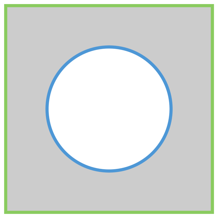
(a) 2D case.

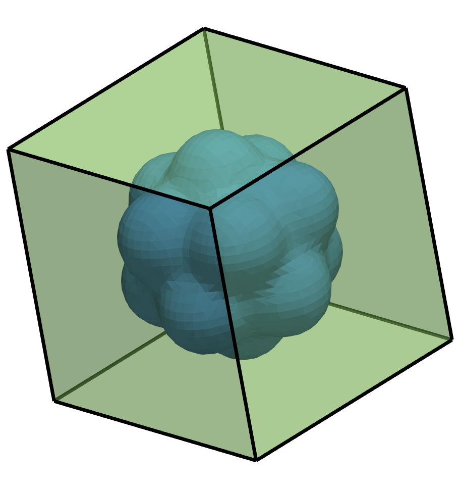
(b) 3D case (outer view).

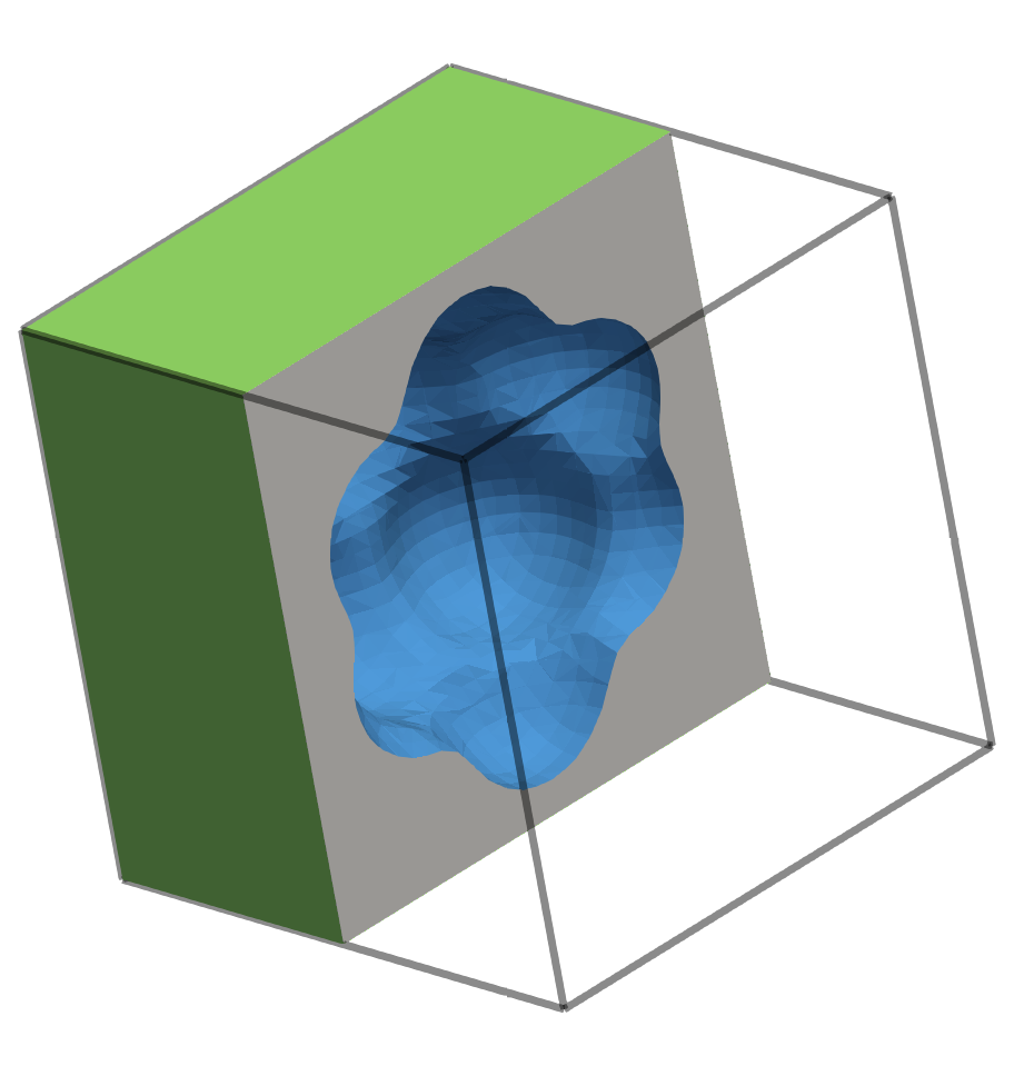
(c) 3D case (internal view).

Figure 5. Convergence test: View of the problem geometries.

We use the method of manufactured solutions in order to have a problem with known exact solution, which is used here to compute discretization errors. The (manufactured) exact solution we have considered is

$$\boldsymbol{u}\doteq\dfrac{\boldsymbol{u}^{*}}{|\boldsymbol{u}^{*}|},\hskip 40.00006ptp\doteq x^{3}y^{3},$$ (109)

where

$$\begin{array}[]{l}\boldsymbol{u}^{*}=\left(-y+0.5,\ x+0.3\right)^{t},\quad(x,y)\in\Omega\subset\mathbb{R}^{2}\quad\text{in 2D,}\\ \boldsymbol{u}^{*}=\left(y-0.5,\ -x-z-0.3,\ y-0.5\right)^{t},\quad(x,y,z)\in\Omega\subset\mathbb{R}^{3}\quad\text{in 3D.}\end{array}$$ (110)

This solution corresponds to a (divergence-free) velocity field of magnitude $1$ that spins around the point $(x,y)=(-0.3,0.5)$ for the 2D case and around the line $(x,y,z)=(-z-0.3,0.5,z)$, $z\in\mathbb{R}$, in 3D (see Fig. 6). The particular value of the boundary conditions (both Dirichlet and Neumann) and external loads are defined such that (109) is the exact solution of the Stokes problem (1).

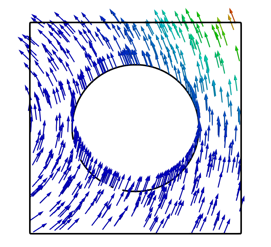
(a) 2D case.

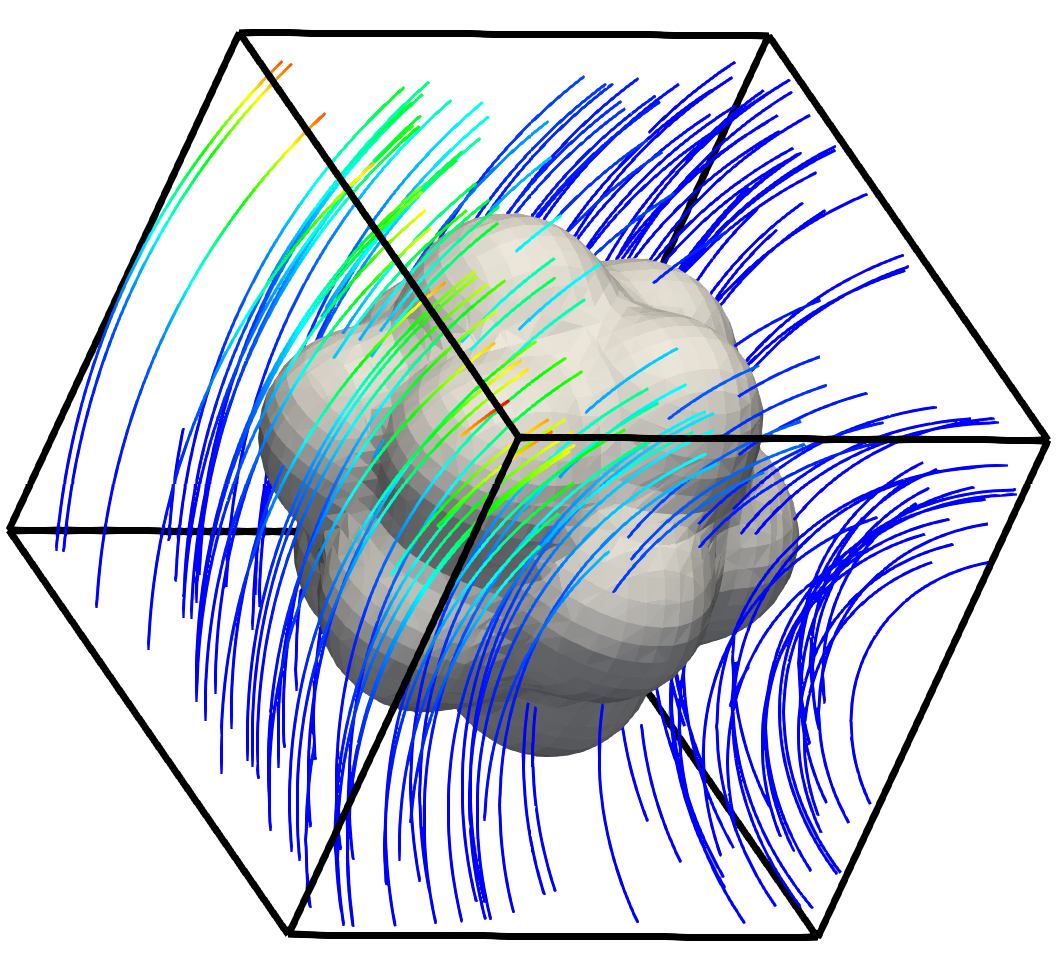
(b) 3D case.

Figure 6. Convergence test: View of the manufactured solution (vectors / streamlines colored by pressure field).

The numerical approximation is done using a family of uniform Cartesian meshes obtained by dividing each direction of the unit square and cube into $2^{m}$ parts, with $m=3,4,\ldots,9$ in 2D, and $m=3,4,5$ in 3D. The obtained results are displayed in Figs. 7, 8, and 9.

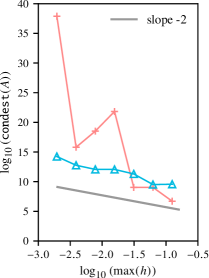
(a) 2D case.

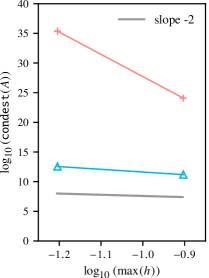
(b) 3D case.

Figure 7. Convergence test: Scaling of the condition number upon mesh refinement.

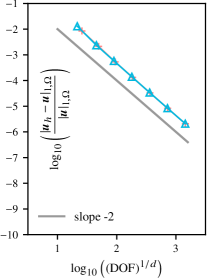
(a) Velocity $H^{1}$ semi-norm.

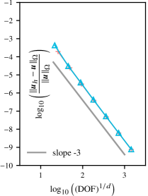
(b) Velocity $L^{2}$ norm.

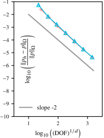
(c) Pressure $L^{2}$ norm.

Figure 8. Convergence test: Convergence of the discretization error for the 2D case ($d=2$).

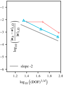
(a) Velocity $H^{1}$ semi-norm.

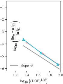
(b) Velocity $L^{2}$ norm.

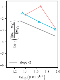
(c) Pressure $L^{2}$ norm.

Figure 9. Convergence test: Convergence of the discretization error for the 3D case ($d=3$).

Fig. 7 shows the scaling of the condition number of the underlying linear systems as the mesh is refined. For the agFE spaces, the condition number scales as expected in conventional FE methods for body-fitted meshes (i.e., the condition number is proportional to $h^{-2}$), which confirms the theoretical condition number bound derived in Sect. 6.4. The same behavior is observed in 2D and 3D cases. The lines for the 3D case in Fig. 7(b) have only two points, since we were able to estimate the condition number only for two of the 3D meshes due to the large amount of memory demanded by the condest function of MATLAB. The benefit of using cell aggregation is clearly illustrated in Fig. 7. The standard FE spaces without cell aggregation lead to condition numbers that do not scale proportional to $h^{-2}$. Theoretically, the condition number can be arbitrary large without cell aggregation depending on how cells are cut, which leads in practice to an erratic scaling of the condition number that reaches large values, as shown by the red lines in Fig. 7.

On the other hand, Figs. 8 and 9 report the convergence of the $H^{1}$ semi-norm and $L^{2}$ norm of the discretization error for the velocity field, and the $L^{2}$ norm of the discretization error for the pressure field for the 2D and 3D cases respectively. Since we consider standard ($\mathcal{Q}_{2,h}(\mathcal{K}_{h})$,${\mathcal{P}}^{-}_{1,h}(\mathcal{K}_{h})$) and aggregated ($\breve{\mathcal{Q}}_{2,h}$,${\mathcal{P}}^{-}_{1,h}$) velocity-pressure elements (which corresponds to $2$nd polynomial order for the velocities and $1$st for the pressures), the optimal convergence orders are $3$rd order of convergence for the velocity error measured in the $L^{2}$ norm, $2$nd order for the velocity error in the $H^{1}$ semi-norm, and $2$nd order for the pressure error in $L^{2}$ norm. The plots show that the agFE spaces lead to these optimal FE convergence orders, which in turn confirms the analysis of Sect. 6.3. Note that the standard (un-aggregated) FE spaces lead to the optimal convergence orders in the 2D case (cf. Fig. 8). However, the underlying linear systems are so ill-conditioned (reaching condition numbers up to $10^{35}$ as previously showed in Fig. 7) that in general one cannot rely on the results computed by the linear solver using double precision floating point arithmetics. We have encountered some situations where the linear solver was not able to provide an accurate solution for this reason, see, e.g., the red line in Fig. 9(c).

7.3. Moving domain experiment

In the second numerical experiment, we study the robustness of the unfitted FE formulation with respect to the relative position between the problem geometry and the background mesh. To this end, we consider two geometries whose definition is parametrized by a scalar value $\ell$ (cf. Fig. 10). The 2D geometry is a circular cavity, with radius $R=0.225$ and whose center is located at an arbitrary point on a diagonal of the unit square (cf. Fig. 10(a)). The 3D domain is again a cavity defined using the popcorn flake geometry (cf. Fig. 10(b)). In this case, We scale down the popcorn flake used in the convergence test (cf. Sect. 7.2) by a factor or $0.5$ and place it at an arbitrary point of the diagonal of the unit cube. In both cases, the position of the bodies is controlled by the value of the parameter $\ell$ (i.e., the distance between the center of the body and a selected vertex of the square/cube). As the value of $\ell$ varies, the objects move and their relative position with respect to the background mesh changes. In this process, arbitrary small cut cells can show up, leading to potential ill conditioning problems. In this experiment, we consider a background mesh that discretizes the unit square/cube with $2^{m}$ elements per direction, being $m=5$ for the 2D case and $m=4$ for the 3D case.

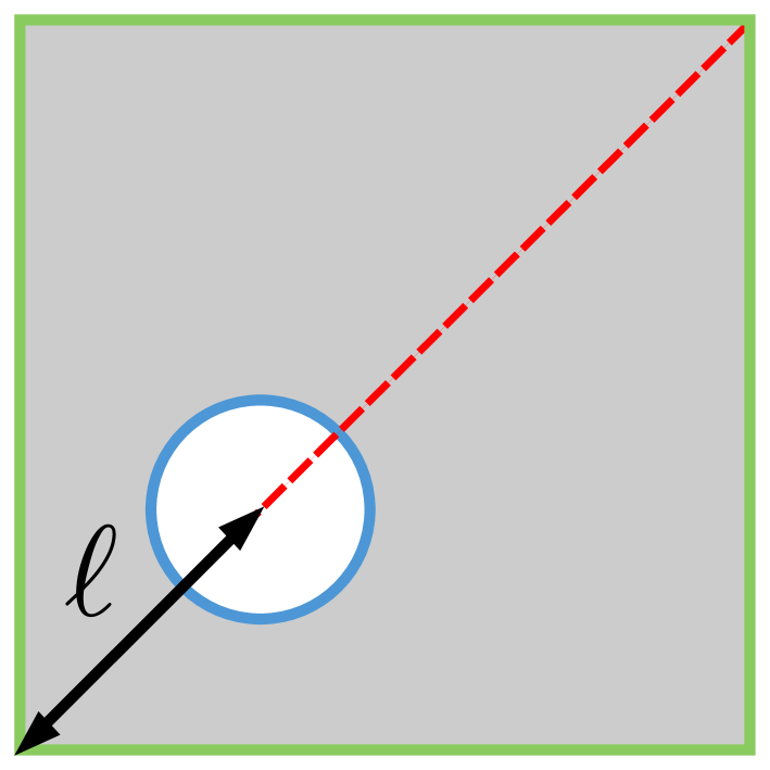
(a) 2D case.

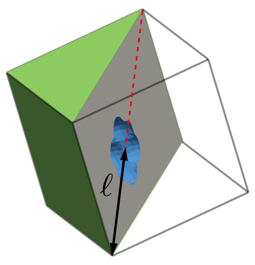
(b) 3D case (internal view).

Figure 10. Moving domain experiment: View of the problem geometries.

Fig. 11 shows the condition number estimate of the underlying linear systems versus $\ell$. The plot is generated using a sample of 200 different values of $\ell$. It is observed that the agFE spaces lead to condition numbers that are nearly independent of the value of $\ell$, which shows that the agFEM is very robust regardless how cells are cut. The benefit of using aggregation is clearly demonstrated here by observing the results associated to the standard FE spaces. In that case, the condition numbers are very sensitive to the position of the geometry and reach very high values (condition number greater than $10^{35}$ in the 3D case).

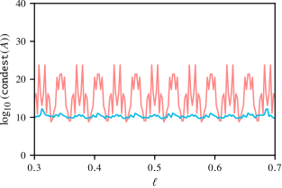
(a) 2D case.

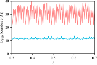
(b) 3D case.

Figure 11. Moving domain experiment: Condition number vs. domain position.

7.4. Complex 3D examples

We conclude the numerical examples with the simulation of two complex geometries in order to show that the cell aggregation can be effectively used also in more complex settings. The first complex example is the simulation of a Stokes flow around a set of randomly spherical obstacles (see Fig. 12). The (fluid) domain is the set difference of the unit cube $[0,1]^{3}$ and the spherical obstacles. We consider homogeneous Dirichlet conditions (no-slip conditions) in the surfaces of the spherical obstacles using Nitsche’s method. The inflow boundary is the face $x=0$ of the unit cube (see Fig. 12(a)), where we impose a prescribed polynomial inflow velocity profile with value:

$$\boldsymbol{u}=(10y(y-1)z(z-1),\ 0,\ 0),\quad(x,y,z)\in\Gamma^{\mathrm{in}}=\{0\}\times[0,1]^{2}.$$ (111)

The outflow boundary is the face $x=1$ of the unit cube, where we impose homogeneous Neumann boundary conditions. We impose homogeneous Dirichlet conditions on the remaining faces of the cube. The problem is simulated using a background Cartesian mesh defined on the cube with $2^{5}$ elements per direction. The obtained numerical solution is plotted in Figs. 12(b) and 12(c). Note that the approximation of the velocities clearly conforms to the unfitted surfaces even though the interpolation is slightly coarsened near these surfaces by the cell aggregation.

Inflow     Outflow

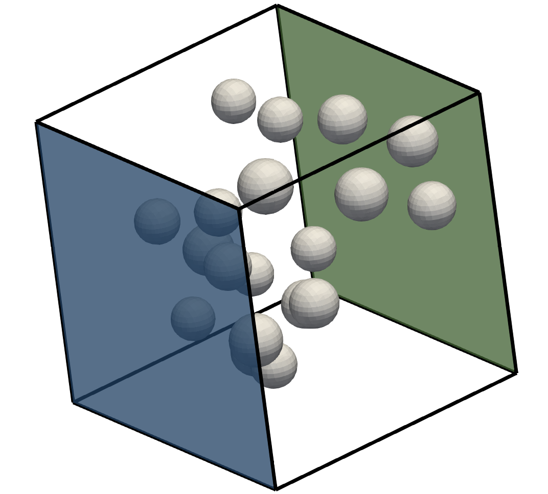
(a) Problem geometry.

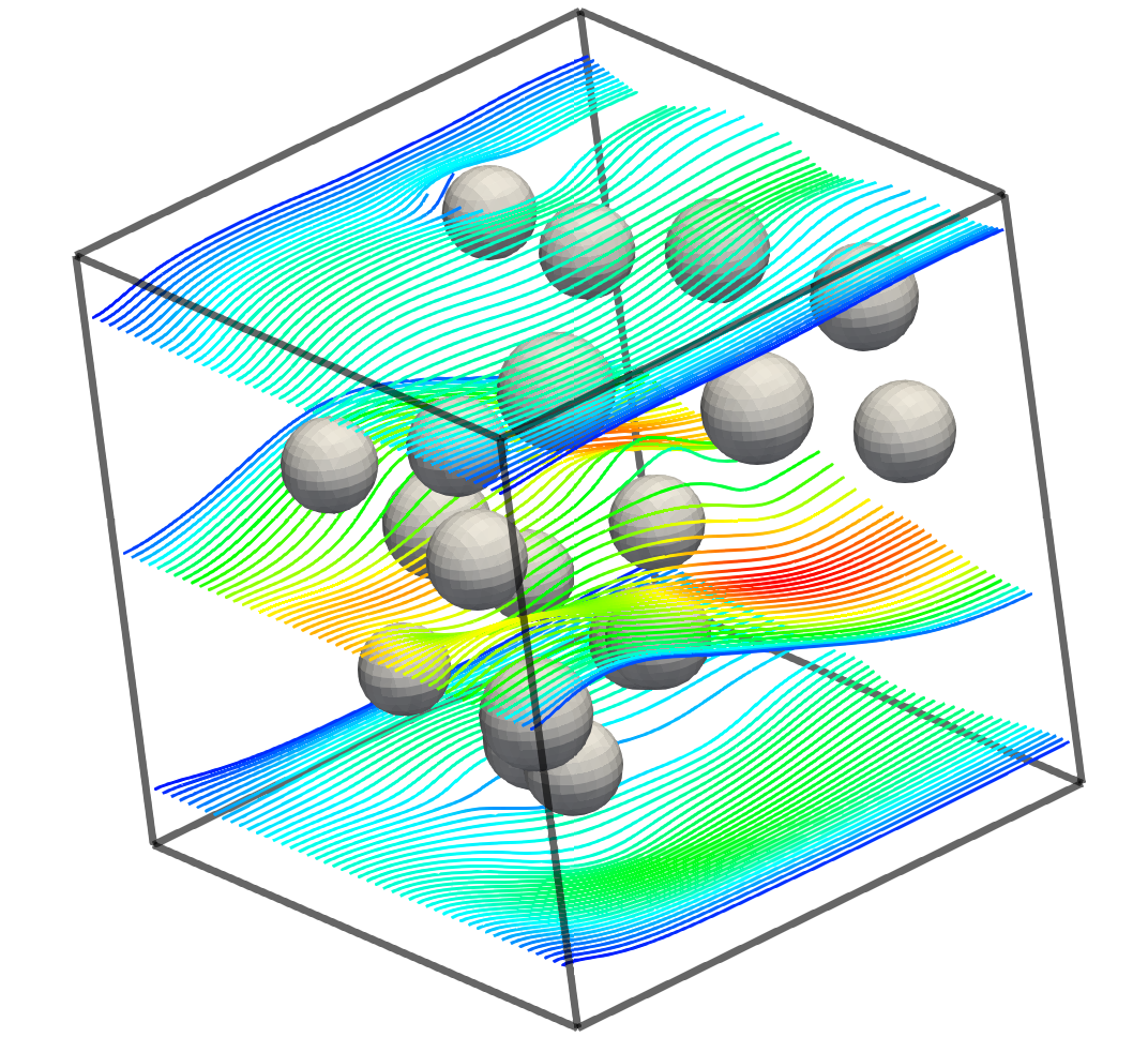
(b) Velocity (magnitude).

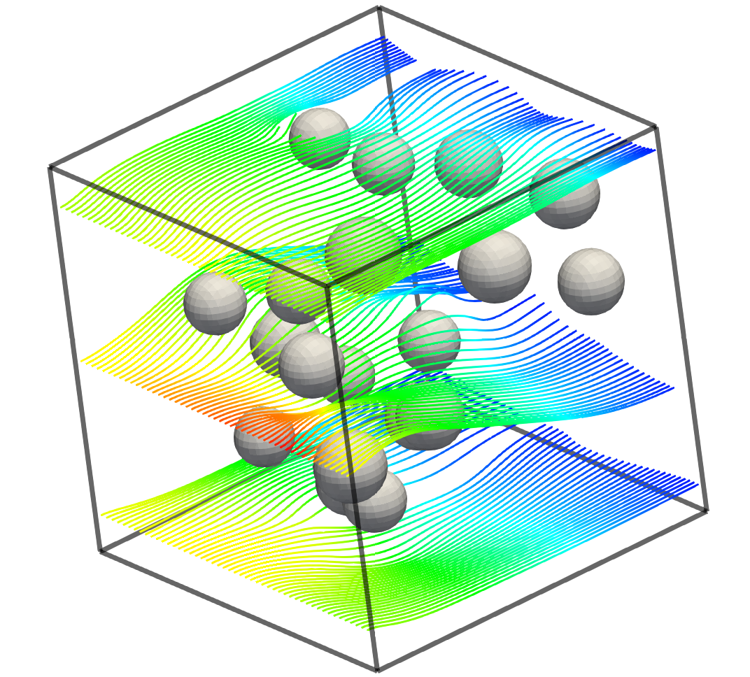
(c) Pressure.

Figure 12. Complex 3D examples: Problem geometry and numerical solution for the stokes flow around spherical obstacles (streamlines colored by velocity magnitude and pressure).

The second complex example is a Stokes flow inside a spiral pipe (see Fig. 13). The radius of the tubular cross section of the pipe is $0.1$, whereas the radius of the spiral central axis is $0.875$. We impose homogeneous Dirichlet conditions on the walls of the spiral. The inflow boundary is one of the two terminal cross sections of the pipe, i.e., the disk of center $C=(0,0.875,0.86)$ and radius $R=0.1$ (see Fig. 13(a)). On the inflow boundary we impose a parabolic velocity profile with value:

$$\boldsymbol{u}=(10-10\frac{r^{2}}{R^{2}},\ 0,\ 0),$$ (112)

where $r\in[0,R]$ is the distance between a point $x$ in the inflow boundary and the center $C$. Homogeneous Neumann boundary conditions are considered on the outflow boundary. Like in the previous example, the problem is simulated using a uniform Cartesian mesh of the unit cube with $2^{5}$ elements at each direction. The results are showed in Figs. 13(b) and 13(c). Note that, even though this is a very challenging example for the cell-aggregation strategy because the surface to volume ratio is very high, the computed results reproduce a perfectly laminar velocity field that flows smoothly through the spiral pipe.

Inflow     Outflow

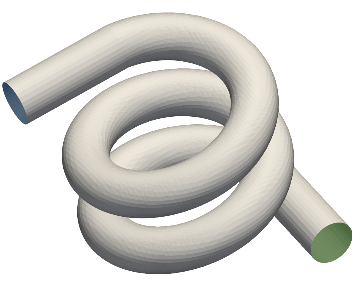
(a) Problem geometry.

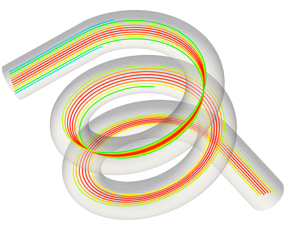
(b) Velocity (magnitude).

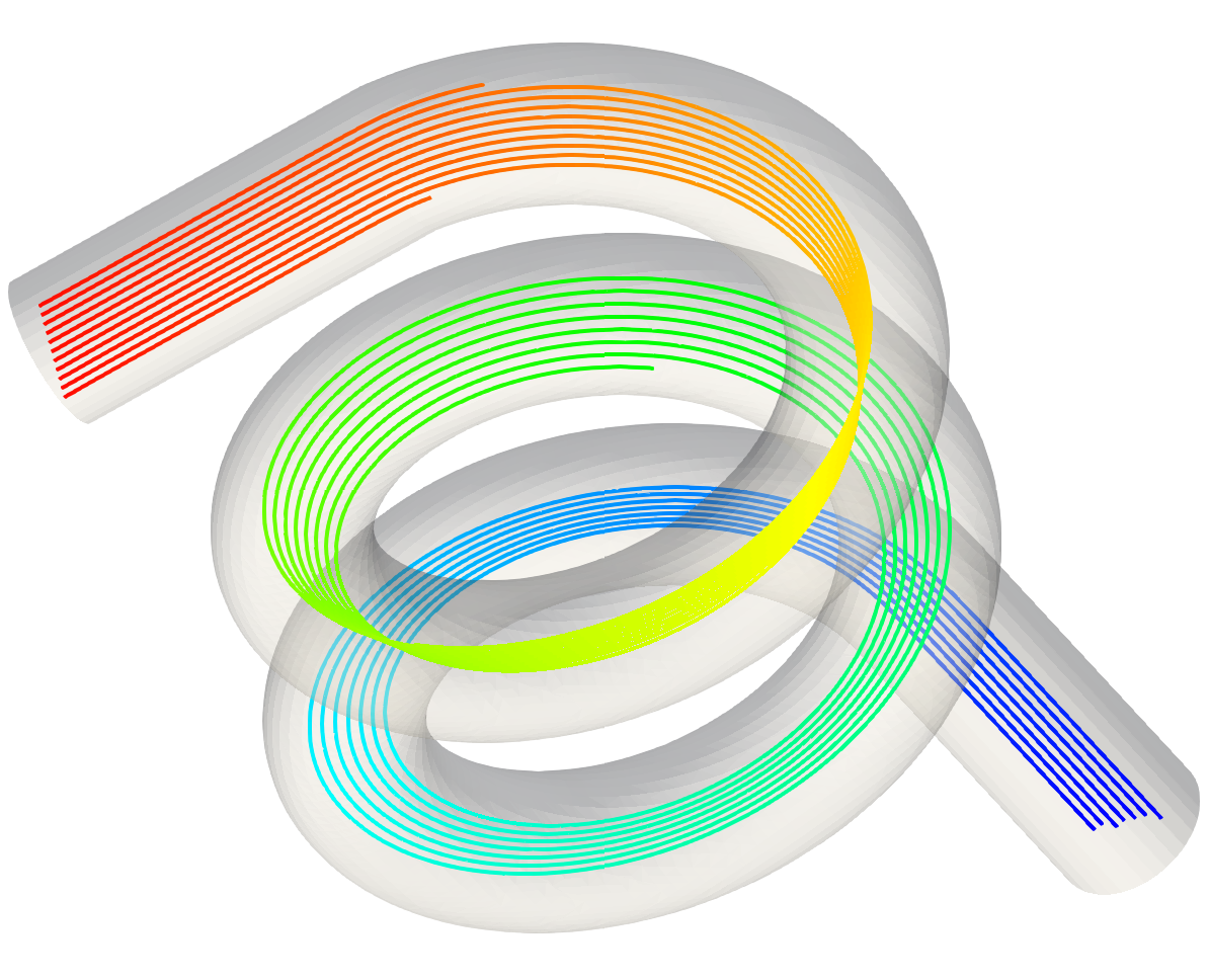
(c) Pressure.

Figure 13. Complex 3D examples: Problem geometry and numerical solution for the stokes flow in a spiral pipe (streamlines colored by velocity magnitude and pressure).

8. Conclusions

In this work, we have developed mixed agFEMs for the approximation of the Stokes problem on unfitted meshes. We have considered the standard extension operator for the definition of agFE spaces and a new one that relies on the extension of the serendipity component only (for hex meshes). A cell aggregation algorithm allows one to start with a FE mesh and create an aggregate partition with some desired properties. The agFE space is readily computed from a typical FE space plus simple cell-wise constraints.

For the sake of conciseness, we have considered as starting point mixed FE methods on body-fitted meshes with discontinuous pressure spaces on hexahedral meshes, considering both the standard and serendipity extension for the velocity field. We have performed an abstract stability analysis that relies on a set of assumptions, in order to prove a weak inf-sup condition for mixed agFE spaces. Such analysis shows the potential deficiency of the unfitted discrete inf-sup for such spaces. It allows us to identify a subset of aggregates/facets (close to the boundary), coined improper aggregates/facets; these subsets depend on the mixed agFE space being used.

Based on the abstract stability analysis, we have defined two different algorithms that satisfy the required assumption for having stability. The first algorithm relies on a standard velocity extension plus interior (residual-based) stabilization in improper aggregates and pressure jump stabilization on improper facets. The second algorithm relies on the serendipity extension for the velocity field components and pressure jump stabilization on improper facets. For these algorithms, a complete numerical analysis proves stability, a priori error estimates, and condition number bounds that are not affected by the small cut cell problem.

A complete set of numerical experiments bears out the numerical analysis. Finally, the mixed agFEM is applied to two problems with non-trivial geometries, viz., free flow in a medium with inclusions and confined flow in a spiral.

References

- Badia et al. [2008] S. Badia, F. Nobile, and C. Vergara. Fluid–structure partitioned procedures based on Robin transmission conditions. Journal of Computational Physics, 227(14):7027–7051, 2008. doi:10.1016/j.jcp.2008.04.006.
- Chiumenti et al. [2017] M. Chiumenti, E. Neiva, E. Salsi, M. Cervera, S. Badia, J. Moya, Z. Chen, C. Lee, and C. Davies. Numerical modelling and experimental validation in Selective Laser Melting. Additive Manufacturing, 18:171–185, 2017. doi:10.1016/j.addma.2017.09.002.
- Belytschko et al. [2001] T. Belytschko, N. Moës, S. Usui, and C. Parimi. Arbitrary discontinuities in finite elements. International Journal for Numerical Methods in Engineering, 50(4):993–1013, 2001. doi:10.1002/1097-0207(20010210)50:4<993::AID-NME164>3.0.CO;2-M.
- Burman et al. [2015] E. Burman, S. Claus, P. Hansbo, M. G. Larson, and A. Massing. CutFEM: Discretizing geometry and partial differential equations. International Journal for Numerical Methods in Engineering, 104(7):472–501, 2015. doi:10.1002/nme.4823.
- de Prenter et al. [2017] F. de Prenter, C. V. Verhoosel, G. J. van Zwieten, and E. H. van Brummelen. Condition number analysis and preconditioning of the finite cell method. Computer Methods in Applied Mechanics and Engineering, 316:297–327, 2017. doi:10.1016/j.cma.2016.07.006.
- Schillinger and Ruess [2014] D. Schillinger and M. Ruess. The Finite Cell Method: A Review in the Context of Higher-Order Structural Analysis of CAD and Image-Based Geometric Models. Archives of Computational Methods in Engineering, 22(3):391–455, 2014. doi:10.1007/s11831-014-9115-y.
- Badia and Verdugo [In press, 2017] S. Badia and F. Verdugo. Robust and scalable domain decomposition solvers for unfitted finite element methods. Computational and Applied Mathematics, In press, 2017.
- Badia et al. [2018a] S. Badia, F. Verdugo, and A. F. Martín. The aggregated unfitted finite element method for elliptic problems. Computer Methods in Applied Mechanics and Engineering, 336:533–553, 2018a.
- Badia et al. [2018b] S. Badia, A. F. Martín, and J. Principe. FEMPAR: An object-oriented parallel finite element framework. Archives of Computational Methods in Engineering, 25(2):195–271, 2018b.
- [10] FEMPAR webpage. http://www.fempar.org/.
- Burman and Hansbo [2012] E. Burman and P. Hansbo. Fictitious domain finite element methods using cut elements: II. A stabilized Nitsche method. Applied Numerical Mathematics, 62(4):328–341, 2012. doi:10.1016/j.apnum.2011.01.008.
- Höllig et al. [2001] K. Höllig, U. Reif, and J. Wipper. Weighted Extended B-Spline Approximation of Dirichlet Problems. SIAM Journal on Numerical Analysis, 39(2):442–462, 2001. doi:10.1137/S0036142900373208.
- Rüberg and Cirak [2012] T. Rüberg and F. Cirak. Subdivision-stabilised immersed b-spline finite elements for moving boundary flows. Computer Methods in Applied Mechanics and Engineering, 209-212:266–283, 2012. doi:10.1016/j.cma.2011.10.007.
- Rüberg and Cirak [2014] T. Rüberg and F. Cirak. A fixed-grid b-spline finite element technique for fluid–structure interaction. International Journal for Numerical Methods in Fluids, 74(9):623–660, 2014. doi:10.1002/fld.3864.
- Helzel et al. [2005] C. Helzel, M. Berger, and R. Leveque. A High-Resolution Rotated Grid Method for Conservation Laws with Embedded Geometries. SIAM Journal on Scientific Computing, 26(3):785–809, 2005. doi:10.1137/S106482750343028X.
- Johansson and Larson [2013] A. Johansson and M. G. Larson. A high order discontinuous Galerkin Nitsche method for elliptic problems with fictitious boundary. Numerische Mathematik, 123(4):607–628, 2013. doi:10.1007/s00211-012-0497-1.
- Kummer [2013] F. Kummer. Extended Discontinuous Galerkin methods for multiphase flows: The spatial discretization. Center for Turbulence Research Annual Research Briefs, pages 319–333, 2013.
- Burman and Hansbo [2014] E. Burman and P. Hansbo. Fictitious domain methods using cut elements: III. A stabilized Nitsche method for Stokes’ problem. ESAIM: Mathematical Modelling and Numerical Analysis, 48(3):859–874, 2014. doi:10.1051/m2an/2013123.
- Hansbo et al. [2014] P. Hansbo, M. G. Larson, and S. Zahedi. A cut finite element method for a {Stokes} interface problem. Applied Numerical Mathematics, 85:90–114, 2014. doi:10.1016/j.apnum.2014.06.009.
- Cattaneo et al. [2015] L. Cattaneo, L. Formaggia, G. F. Iori, A. Scotti, and P. Zunino. Stabilized extended finite elements for the approximation of saddle point problems with unfitted interfaces. Calcolo, 52(2):123–152, 2015. doi:10.1007/s10092-014-0109-9.
- Guzmán and Olshanskii [2017] J. Guzmán and M. Olshanskii. Inf-sup stability of geometrically unfitted Stokes finite elements. Mathematics of Computation, page 1, 2017. doi:10.1090/mcom/3288.
- Massing et al. [2014] A. Massing, M. G. Larson, A. Logg, and M. E. Rognes. A Stabilized Nitsche Fictitious Domain Method for the Stokes Problem. Journal of Scientific Computing, 61(3):604–628, 2014. doi:10.1007/s10915-014-9838-9.
- Burstedde et al. [2011] C. Burstedde, L. C. Wilcox, and O. Ghattas. p4est: Scalable algorithms for parallel adaptive mesh refinement on forests of octrees. SIAM Journal on Scientific Computing, 33(3):1103–1133, 2011. doi:10.1137/100791634.
- Brezis [2010] H. Brezis. Functional Analysis, Sobolev Spaces and Partial Differential Equations. Springer, 2010.
- Arnold and Awanou [2011] D. N. Arnold and G. Awanou. The Serendipity Family of Finite Elements. Foundations of Computational Mathematics, 11(3):337–344, 2011. doi:10.1007/s10208-011-9087-3.
- Arnold et al. [2000] D. N. Arnold, D. Boffi, and R. S. Falk. Approximation by quadrilateral finite elements. Mathematics of Computation, 71(239):13, 2000. doi:10.1090/S0025-5718-02-01439-4.
- Brenner and Scott [2010] S. C. Brenner and R. Scott. The Mathematical Theory of Finite Element Methods. Springer, softcover reprint of hardcover 3rd ed. 2008 edition, 2010.
- Johansson and Larson [2013] A. Johansson and M. G. Larson. A high order discontinuous Galerkin Nitsche method for elliptic problems with fictitious boundary. Numerische Mathematik, 123(4):607–628, 2013. doi:10.1007/s00211-012-0497-1.
- Hansbo and Hansbo [2002] A. Hansbo and P. Hansbo. An unfitted finite element method, based on Nitsche’s method, for elliptic interface problems. Computer methods in applied mechanics and engineering, 191(47):5537–5552, 2002. doi:10.1016/S0045-7825(02)00524-8.
- Scott and Zhang [1990] L. R. Scott and S. Zhang. Finite Element Interpolation of Nonsmooth Functions Satisfying Boundary Conditions. Mathematics of Computation, 54(190):483–493, 1990. doi:10.2307/2008497.
- Ern and Guermond [2004] A. Ern and J.-L. Guermond. Theory and Practice of Finite Elements. Springer, 2004.
- Becker [2002] R. Becker. Mesh adaptation for Dirichlet flow control via Nitsche’s method. Communications in Numerical Methods in Engineering, 18(9):669–680, 2002. doi:10.1002/cnm.529.
- Nitsche [1971] J. Nitsche. Über ein Variationsprinzip zur Lösung von Dirichlet-Problemen bei Verwendung von Teilräumen, die keinen Randbedingungen unterworfen sind. Abhandlungen aus dem Mathematischen Seminar der Universität Hamburg, 36(1):9–15, 1971. doi:10.1007/BF02995904.
- Bernardi et al. [2016] C. Bernardi, M. Costabel, M. Dauge, and V. Girault. Continuity Properties of the Inf-Sup Constant for the Divergence. SIAM Journal on Mathematical Analysis, 48(2):1250–1271, 2016. doi:10.1137/15M1044989.
- Elman et al. [2005] H. C. Elman, D. J. Silvester, and A. J. Wathen. Finite elements and fast iterative solvers: with applications in incompressible fluid dynamics. Oxford University Press, 2005.
- [36] Intel MKL PARDISO - Parallel Direct Sparse Solver Interface. https://software.intel.com/en-us/articles/intel-mkl-pardiso.
- [37] QHULL webpage. http://www.qhull.org/.
- Barber et al. [1996] C. B. Barber, D. P. Dobkin, and H. Huhdanpaa. The Quickhull algorithm for convex hulls. ACM Transactions on Mathematical Software, 22(4):469–483, 1996.