Non-linear model and optimization method for a single-axis linear-motion energy harvester for footstep excitation

Michael N. Struwig, Riaan Wolhuter, Thomas Niesler

Abstract

We propose and develop an electrical and mechanical system model of a single-axis linear-motion kinetic energy harvester for impulsive excitation that allows its generated load power to be numerically optimised as a function of design parameters. The device consists of an assembly of one or more spaced magnets suspended by a magnetic spring and passing through one or more coils when motion is experienced along the axis. The design parameters that can be optimised include the number of coils, the coil height, coil spacing, the number of magnets, the magnet spacing and the physical size. We use the proposed model to design optimal energy harvesters for the case of impulse-like motion like that experienced when attached to the leg of a human. We generate several optimised designs, ranked in terms of their predicted load power output. The three best designs are subsequently constructed and subjected to controlled practical evaluation while attached to the leg of a human subject. The results show that the ranking of the measured output power corresponds to the ranking predicted by the optimisation, and that the numerical model correctly Predicts the relative differences in generated power for complex motion. It is also found that all three designs far outperform a baseline design. The best energy harvesters generated an average power of 3.01mW into a 40$\Omega$ test load when driven by footsteps whose measured peak impact was approximately 2.2g. With respect to the device dimensions, this corresponds to a power density of 179.380$\mu\text{W/cm}^{3}$.

Keywords: kinetic energy harvesting, magnetic spring, optimization, footstep

Declaration of interest: none.

1 Introduction

Energy harvesting has become an increasingly popular field as researchers and industry alike attempt to discover and improve ways of powering electrical devices in situations where conventional sources of power are unavailable [1] [2] [3]. One source is kinetic energy, where the mechanism of electromagnetic induction is used to generate electrical energy [4]. The literature has described a wide variety of electromagnetic kinetic microgenerators, many of which are modelled as linear spring-damper systems that harvest energy from sources of harmonic vibration [5] [6] [7]. More recently, increasingly complex non-linear models have been proposed in a quest to harvest energy from a wider variety of kinetic sources [8] [9] [10]. However, for both linear and non-linear models, the analysis based on electromagnetic first principles results in a significant degree of mathematical complexity and requires the use of parameters that are difficult to determine [11]. This has hindered the development of techniques that allow the parametric optimization of kinetic energy harvesting beyond resonant-frequency optimization and resistive load matching [12] [13]. When parametric optimization is performed, it is typically in the form of experimental iteration [14] [15], or considers a very limited number of parameters [16] [17].

In contrast to harmonic vibration, very little attention has been given to energy harvesters driven by impulse-like accelerations [18]. This currently severely limits the design of a kinetic energy harvesting device for an environment in which the primary source of energy is impulse-like acceleration, such as that resulting from the footstep of a person or animal. Methods developed for harmonic vibration cannot accurately be applied in these situations.

The initial motivation for the work we present here was to enable the design of self-powering animal-borne sensors for use in the monitoring and conservation of large wildlife. In this situation, the source of energy is the impulse-like motion of the animal’s leg, while severe size and weight limitations make it essential to maximize the harvested energy. Despite major advancement in the sophistication of animal-tracking collars, such as the inclusion of GPS, on-board data transmission and on-board behaviour classification [19], battery life remains the greatest limitation [20] [21].

We propose a non-linear mechanical model for a single-axis electromagnetic kinetic microgenerator that allows the constrained parametric optimization of design parameters in order to maximize the average power supplied to the attached load. This is achieved by developing an electrical model for a simplified configuration of the energy harvesting device for a form of non-harmonic motion. This model is applied to the analysis of more complex configurations, thereby providing a means of optimizing the microgenerator design. It should be noted that despite sharing similar architecture features, the proposed model and optimization methodology differs significantly from those typically found in literature [22] due to the focus on harvesting energy from non-vibrational sources. Additionally, our approximate analytical model is in contrast to the use of first-principle electromagnetic techniques previously proposed [23][24] and offers the advantage of much greater computational speed, once defined, in comparison to performing a simulation with finite element analysis (FEA) due to the proposed model’s parametric nature. We demonstrate the effectiveness of our method by using it to determine a number of optimal microgenerator designs, and subsequently constructing and practically evaluating these for footstep input.

2 Microgenerator architecture

The kinetic energy harvester we consider consists of a hollow circular tube, inside of which a set of one or more magnets is able to move, as illustrated in Fig. 1. The primary axis is parallel to the limb of the person or animal. A number of uniformly spaced coils are wound around the outside of the tube. The magnet assembly consists of a number of permanent magnets that are arranged with alternating polarity and separated by a spacer of some ferrous material. A fixed pole-matched magnet is placed at the bottom of the tube. This non-linear magnetic spring allows the magnet assembly to oscillate and for gravity to reset its position after motion. The non-linear characteristic of the magnet spring increases model complexity, but affords several benefits. Firstly, the non-linear spring can push the magnet assembly upwards, but cannot pull it downwards, thereby increasing the range of motion of the magnet assembly. Secondly, the magnetic spring is more consistent and less prone to mechanical failure than a mechanical spring, which is of critical importance for our eventual intended application in wildlife monitoring. Finally, it is simpler to assemble, as the magnetic spring consists of the same type of magnet used in the magnet assembly, and does not require manufacture or sourcing of a specialized mechanical spring.

Once selected, the properties of the individual permanent magnets, copper wire and winding density are considered to be fixed. The remaining variables, which include the footstep forces, coil height, electrical load, number of magnets, number of coils and various coil properties are varied to optimize the design of the kinetic energy harvester.

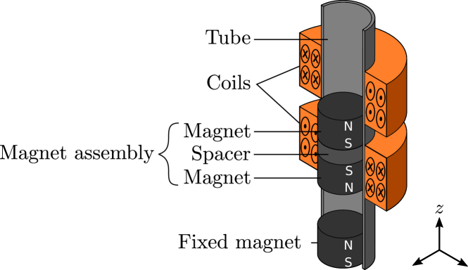
Figure 1: Basic structure of the linear kinetic energy harvester, showing multiple coils and multiple magnets. The magnets and coils are pole-matched. A single fixed magnet at the base provides a magnetic spring.

3 Analytical models for microgenerator optimization

This section develops an analytical model for the kinetic energy harvester. The model consists of a mechanical system model, describing the mechanical responses of the kinetic energy harvester, the footstep model that drives the mechanical model and an electrical system model that describes the electrical output.

3.1 Footstep model

The acceleration $a_{\text{step}}$ of the footstep is modelled as a piece-wise constant non-periodic function, given by Eq. 1 and shown graphically in Fig. 2. This model is based on a simplified footstep cycle using measurements taken from an accelerometer attached to the leg of a human when walking and aligned with corresponding video footage. The constant accelerations $a_{\text{up}}$, $a_{\text{dec}}$, $a_{\text{down}}$ and $a_{\text{impact}}$ respectively represent the average acceleration experienced by the microgenerator body during the upstroke, deceleration, downstroke and impact phases of a single footstep cycle as shown in Fig. 3.

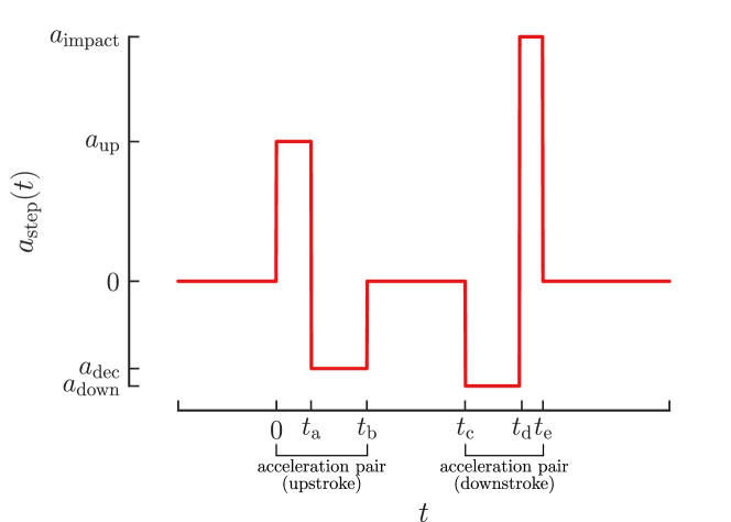
Figure 2: The footstep is modelled as two acceleration pairs; one for the upstroke and another for the downstroke. The two stroke pairs are separated by the time interval $t_{\text{b}}<t\leq t_{\text{c}}$.

$$a_{\text{step}}(t)=\begin{cases}a_{\text{up}},&\text{for}\ 0\leq t\leq t_{\text{a}}\\ a_{\text{dec}},&\text{for}\ t_{\text{a}}<t\leq t_{\text{b}}\\ 0,&\text{for}\ t_{\text{b}}<t\leq t_{\text{c}}\\ a_{\text{down}},&\text{for}\ t_{\text{c}}\leq t\leq t_{\text{d}}\\ a_{\text{impact}},&\text{for}\ t_{\text{d}}<t\leq t_{\text{e}}\\ 0,&\text{for}\ t_{\text{e}}<t,\end{cases}$$ (1)

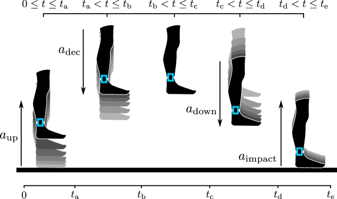
Figure 3: Shows the motion of the leg at different stages during the footstep cycle and the resulting direction of acceleration experience by the kinetic microgenerator body.

Assuming the foot to be motionless in the $z$-direction at $t=0$ and again at $t=t_{\text{b}}$, $t_{\text{a}}$ and $t_{\text{b}}$ can be calculated from the kinematic equations of motion.

$$t_{\text{a}} =\sqrt{\frac{2a_{\text{dec}}s_{\text{h}}}{a_{\text{up}}(a_{\text{dec}}-a_{\text{up}})}}$$ (2)

$$t_{\text{b}} =\frac{2s_{\text{h}}}{a_{\text{up}}t_{\text{a}}}\left(1+\frac{a_{\text{dec}}}{a_{\text{up}}-a_{\text{dec}}}\right)+t_{\text{a}}.$$ (3)

Assuming further that the foot is motionless in the $z$-direction at $t=t_{\text{c}}$ and again at $t=t_{\text{e}}$, analogous equations can be written for $t_{\text{d}}$ and $t_{\text{e}}$ in terms of $a_{\text{down}}$ and $a_{\text{impact}}$. In this way the values of $a_{\text{up}},a_{\text{dec}},a_{\text{down}}$ and $a_{\text{impact}}$ as well as the maximum vertical displacement $s_{\text{h}}$ can be selected to match any practically measurable footstep-like motion.

The piecewise-constant acceleration approximation shown in Fig. 2 was adopted for two reasons. Firstly, the utilized accelerometer data was sampled at 40Hz, which is too sparse to use directly when computing a numerical solution for Eq. 4. Secondly, by selecting the acceleration values of each phase of the footstep to match measured accelerometer data, $a_{\text{step}}(t)$ can approximate a wide variety of footstep-like motion, which potentially opens up the device’s application in other fields, such as energy harvesting on wildlife.

3.2 Mechanical system model

The device in Fig. 1 is modelled by a mechanical system consisting of a mass $M_{\text{mag}}$ representing the magnet assembly attached to the bottom of the outer tube via a non-linear magnetic spring with force $\delta_{\text{mag}}$ and a damper representing energy losses that are proportional to the relative velocity between the magnet assembly and the tube with constant $b_{\text{damper}}$. Similar models have been used to design energy harvesters, but these employ a linear spring $\delta_{\text{spring}}$ to facilitate the oscillatory motion of the magnet assembly [16] [25] [26]. In contrast, our design makes use of a magnetic spring $\delta_{\text{mag}}$. This differs from other work in the literature that utilize a magnetic spring [11] [22] , as we utilize a single repelling magnet at the bottom of the device, as shown in Fig. 1. The resulting mechanical model of the system is shown in Fig. 4.

Figure 4: Idealized mechanical model of microgenerator. The mass of the magnet assembly $M_{\text{mag}}$ is suspended by the nonlinear magnetic spring $\delta_{\text{mag}}$ and experiences mechanical losses through friction with constant $b_{\text{damper}}$ through the walls of the tube.

The value $z_{\text{m}}(t)$ represents the position of the magnet assembly relative to the bottom of the magnet in the assembly and $z_{\text{t}}(t)$ represents the position of the microgenerator tube relative to the top of the fixed magnet. The magnetic spring force $\delta_{\text{mag}}$ is a non-linear function of the relative displacement between the magnet assembly and the tube. The mechanical system can be reduced to a set of first-order differential equations by defining $x_{1}=z_{\text{m}}$, $x_{2}=\dot{z_{\text{m}}}$, $x_{3}=z_{\text{t}}$, $x_{4}=\dot{z_{\text{t}}}$, to find:

$$\begin{bmatrix}\dot{x_{1}}\\ \dot{x_{2}}\\ \dot{x_{3}}\\ \dot{x_{4}}\\ \end{bmatrix}=\begin{bmatrix}x_{2}\\ \big{(}\delta_{\text{mag}}(x_{1}-x_{3})+b_{\text{damper}}\cdot(x_{2}-x_{4})\big{)}/M_{\text{mag}}\\ x_{4}\\ a_{\text{step}}(t)\end{bmatrix}.$$ (4)

To solve Eq. 4, the continuous function $\delta_{\text{mag}}$ and the function $a_{\text{step}}$ must be known. The force between two permanent magnets as a function of the distance between them is difficult to determine analytically because it requires a knowledge of quantities that are extremely difficult to describe, such as the $B-$field vector of magnetic flux density, the vector of the magnetic dipole moment $m$, and the interactions of these properties between the two magnets [27].

We propose a simple approximation of $\delta_{\text{mag}}(z)$ that can be obtained by considering Coulomb’s Law, which can be used to describe the force between two hypothetical magnetic monopoles of strength $m_{1}$ and $m_{2}$ as inversely proportional to the squared distance $r$ between them.

$$\delta_{\text{mag}}(z) =\frac{\mu_{0}m_{1}m_{2}}{4\pi z^{2}}$$ (5)

For comparison, we consider a power series model that is commonly utilized in literature to model the force between two magnets [28]:

$$\delta_{\text{mag}}(z)=\sum_{n=0}^{3}a_{n}z^{n}.$$ (6)

Discrete values of $\delta_{\text{mag}}(z)$ can be obtained by simulation using FEA analysis of two identical cylindrical magnets aligned vertically along their N-S axes such that their poles are matched. The force experienced by the second magnet can then be obtained using FEA for a discrete set of separating distances $z$. The results of such a simulation are compared with the approximation given by Eqs. 5 and 6 in Fig. 5 for constants of $m_{1}=m_{2}=4.119\text{A}\cdot\text{m}$ in the case of Eq. 5 and for coefficients $a_{o}=$1.709\text{\times}{10}^{1}$,~{}a_{1}=$-1.713\text{\times}{10}^{03}$,~{}a_{2}=$5.082\text{\times}{10}^{04}$~{}\text{and}~{}a_{3}=$-4.594\text{\times}{10}^{05}$$ in the case of Eq. 6. The constants and coefficients are found using a typical least-squares curve-fit procedure.

We see that the power series approximation gives a poor approximation of the force between two magnets in our case. We also see that, while the approximation is poor when the magnets are close together, the Coulomb’s Law approximation is good when the magnets are far apart.

Figure 5: The repelling force between two pole-matched cylindrical N35-grade NdFeB magnets with height of 10mm and a radius of 5mm. The power series model provides a generally poor approximation for the true force between two magnets at all distances. In contrast, Coulomb’s Law provides a poor approximation when the two magnets are close to one another, yet is accurate when they are far apart. By including the additional parameter $G$ in the denominator of Coulomb’s Law, a much better correspondence with FEA is achieved for smaller separation distances $z$.

To improve the approximation given by Coulomb’s Law, we modify Eq. 5 as shown in Eq. 7, creating a modified version of Coulomb’s Law:

$$\delta_{\text{mag}}(z)=\frac{\mu_{0}m_{1}m_{2}}{4\pi z^{2}+G}.$$ (7)

The constant parameter $G$ sharpens the knee of the original Coulomb’s Law curve for small values of $z$, and is determined by fitting Eq. 7 to values of $\delta_{\text{mag}}$ obtained by numerical simulation, giving $m_{1}=m_{2}=15.302\text{A}\cdot{m}$ and $G=$1.125\text{\times}{10}^{-4}$$. This provides a much better approximation of the true value of $\delta_{\text{mag}}$ in a closed form, shown in Fig. 5 , which will allow FEA to be sidestepped later.

3.3 Electrical system model

The primary goal of the electrical system model is to describe the power delivered to the load, parameterized in terms of a set of important design parameters. A model will first be developed to describe the idealized movement of a single magnet passing through a single coil at a constant velocity. Subsequently, this will be extended to include configurations with multiple coils and multiple magnets for the same type of movement. Finally, it will be demonstrated that the estimated power produced with this simple motion is representative of the true power that produced when the device is operated practically in the field.

Figure 6: The kinetic microgenerator powering a load is modelled as a voltage source and two resistors connected in series. The first resistor, $R_{\text{mcrg}}$, represents the internal resistance of the kinetic microgenerator and the second, $R_{\text{load}}$, represents the load. The voltage $e(t)$ represents the instantaneous open-circuit EMF produced by the kinetic microgenerator in volts.

A resistive load $R_{\text{load}}$ in series with a kinetic microgenerator with internal resistance $R_{\text{mcrg}}$, as shown in Fig. 6, dissipates an instantaneous power $P_{\text{load}}(t)$ in the load as given by

$$P_{\text{load}}(t)=V_{\text{load}}(t)^{2}/R_{\text{load}}$$ (8)

where it can be shown that

$$V_{\text{load}}(t)=e(t)\frac{R_{\text{load}}}{R_{\text{load}}+R_{\text{mcrg}}}$$ (9)

and where $e(t)$ is the instantaneous open-circuit EMF produced by the kinetic microgenerator, in volts. The RMS power $\bar{P}_{\text{load}}$ delivered to the load is then given by:

$$\bar{P}_{\text{load}}=\frac{e^{2}_{\text{RMS}}R_{\text{load}}}{(R_{\text{mcrg}}+R_{\text{load}})^{2}}.$$ (10)

Hence, by modeling $e(t)$ and $R_{\text{mcrg}}$, $P_{\text{load}}$ and $\bar{P}_{\text{load}}$ can be determined.

3.3.1 Single coil, single magnet configuration

We first consider the case of a kinetic microgenerator consisting of a single coil and a single magnet, before extending the analysis to a more general case.

Figure 7 shows a coil defined by three primary parameters; the turn density $\gamma$ (measured in turns per mm), the height of the coil $h$ (measured in mm) and the resistance per turn $\beta$ (measured in Ohms per turn). The turn density is given by

Figure 7: Cross section of microgenerator body and coil with square tiling of turns. The coil consists of $N$ number of packed turns, with wire radius $r_{\text{c}}$, creating a coil with thickness $c_{\text{th}}$ and height $h$.

$$\gamma =\frac{N}{h_{\text{unit}}}$$

$$=f_{\text{f}}\frac{c_{\text{th}}}{\pi r^{2}_{\text{c}}},$$ (11)

where $N$ is the number of packed coil turns, $f_{\text{f}}=0.7$ is the fill factor ratio of the turns, $c_{\text{th}}$ is the coil thickness in mm and $r_{\text{c}}$ is the radius of the copper wire in mm.

Assuming square tiling of the turns, the coil resistance $R_{\text{coil}}$ is given by

$$R_{\text{coil}}=N\pi R_{\text{gauge}}(2r+2r_{\text{c}}+c_{\text{th}}),$$ (12)

where $R_{\text{gauge}}$ is the resistance per unit length of the copper wire in $\mathrm{\SIUnitSymbolOhm}\text{\,}{\mathrm{mm}}^{-1}$. From Eq. 12, the resistance per turn $\beta$ in mm is given by:

$$\beta =\frac{R_{\text{coil}}}{N}$$

$$=\pi R_{\text{gauge}}(2r+2r_{\text{c}}+c_{\text{th}}).$$ (13)

Combining Eq. 11 and Eq. 13 allows the coil resistance to be expressed in terms of all coil parameters:

$$R_{\text{coil}}=\beta\gamma h.$$ (14)

With the coil model defined, we consider the effect of the coil height $h$ on the open-circuit EMF $e(t)$. This is achieved by varying $h$ while keeping all other coil parameters constant. With the magnetic field vector $\vec{\boldsymbol{B}}$ known, an expression for $e(t)$ can be derived using the concept of motional EMF,

$$e(t)=\int_{c}(\vec{\boldsymbol{u}}\times\vec{\boldsymbol{B}})\cdot\vec{dl}_{c},$$ (15)

where $\vec{\boldsymbol{u}}$ is the velocity of a conductor moving through magnetic field $\vec{\boldsymbol{B}}$ with elemental length $\vec{dl}$ and where $c$ indicates the path of integration. Alternatively, Faraday’s law of induction can be used to derive an expression for the EMF.

$$e(t)=-\frac{d}{dt}\int_{s}\vec{\boldsymbol{B}}\cdot d\vec{\boldsymbol{s}},$$ (16)

where $d\vec{\boldsymbol{s}}$ is the infinitesimal surface element of a surface $s$ enclosed by the conductor. However, the analytic solutions of Eqs. 15 and 16 for the problem at hand are prohibitively complex. Hence the characteristics of $e(t)$ will be investigated numerically using FEA.

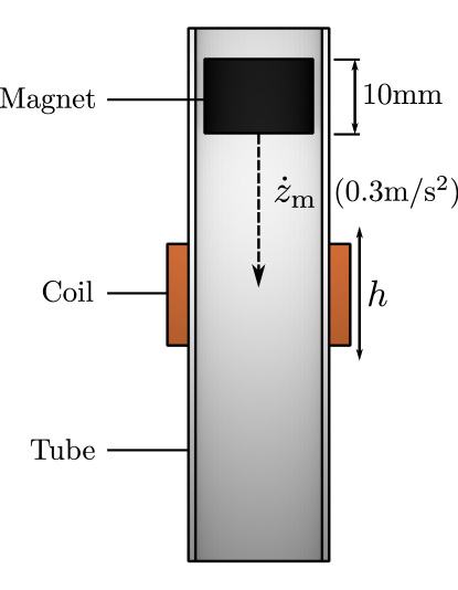
Figure 8: The FEA model used to determine the effect of $h$ on the open-circuit EMF $e(t)$ of a single coil, single magnet kinetic microgenerator.

To do this, we consider the idealized simple transient model shown in Fig. 8. The model consists of a single-magnet, single-coil microgenerator, in which the magnet is assumed to pass through the coil with a constant velocity. Figure 9 shows the result of numerical simulations, by means of FEA, for a range of values of $h$, while a constant velocity $\dot{z}_{\text{m}}=0.3\text{m/s}^{2}$ is used as well as constant values for the parameters $c_{\text{th}},\gamma,\beta$ and the magnet properties. We see that the induced EMF consists of a pulse of positive amplitude followed by one of negative amplitude. These positive and negative pulses occur as the magnet enters and exits the coil, respectively. The zero-crossing occurs at the instant the magnet is at the centre of the coil and the rate of change of flux becomes zero.

Figure 9: FEA of the open-circuit EMF produced by a single-coil, single magnet design for varied $h$ when $\dot{z}_{\text{m}}=0.3\text{m/s}^{2}$.

It can be seen that both the shape and the peak amplitudes of the waveform change substantially with $h$, making it difficult to infer the effect of $h$ on $e(t)$ directly. Instead we consider the RMS of the FEA waveforms shown in Fig. 9. It was found empirically that this RMS voltage can be approximated by Eq. 17, with the constants $A$ and $\alpha$ found from the FEA for the values of $h$ in question. A comparison of the RMS voltage values obtained by FEA and the $e_{\text{RMS}}(h)$ estimated using Eq. 17 is shown in Fig. 10.

$$e_{\text{RMS}}(h)=A\cdot(1-\exp{(-\alpha h)}).$$ (17)

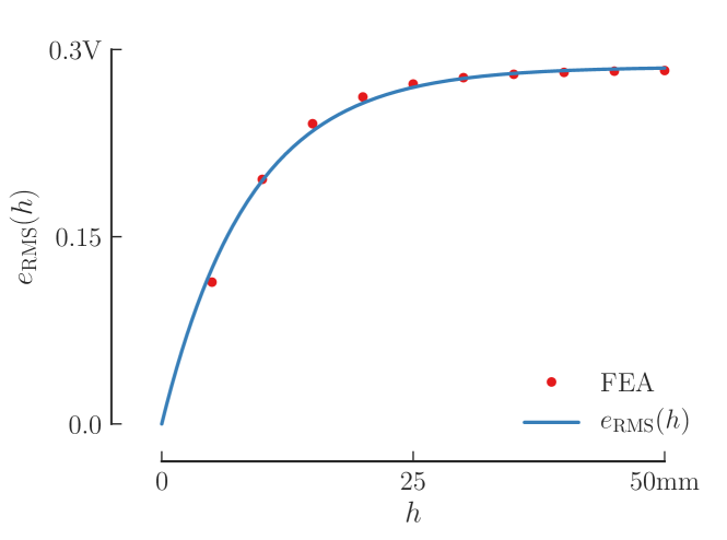
Figure 10: Equation 17 approximates the open-circuit EMF, as a function of the coil height, produced by a single-coil, single-magnet microgenerator.

For a given set of coil parameters $c_{\text{th}}$, $\gamma$, $\beta$ and a given magnetic field, the results in Fig. 10 show that the open-circuit RMS EMF rapidly increases with $h$ before approaching a constant value. This indicates that the coil height $h$ strongly influences the amount of harvestable energy up to a point, after which further increases provide ever diminishing returns.

As a next step, we approximate the waveforms shown in Fig. 9 by the superposition $E(t)$ of two half periods of a sinusoid with period $T_{e}$, as shown in Fig. 11 and described by Eq. 18.

$$E(t)=\begin{cases}V_{\text{p}}\sin{\frac{2\pi}{T_{e}}(t-t_{1})},&\text{for }t_{1}\leq t\leq t_{1}+T_{e}/2\\ -V_{\text{p}}\sin{\frac{2\pi}{T_{e}}(t-t_{2})},&\text{for }t_{2}\leq t\leq t_{2}+T_{e}/2\\ 0,&\text{otherwise}.\end{cases}$$ (18)

The positive half-period in Eq. 18, beginning at $t_{1}$, approximates the EMF generated as the magnet enters the coil, and the negative half-period, beginning at $t_{2}$, approximates the EMF generated as the magnet exits the coil. Equation 18 is zero when the rate of change of flux in the coil is zero. This occurs when the magnet is not in close proximity to the coil (before $t=t_{1}$ and after $t=t_{2}+T_{e}/2$) or when the magnet is approximately centered within the coil at $t_{1}\leq t\leq t_{2}+T_{e}/2$.

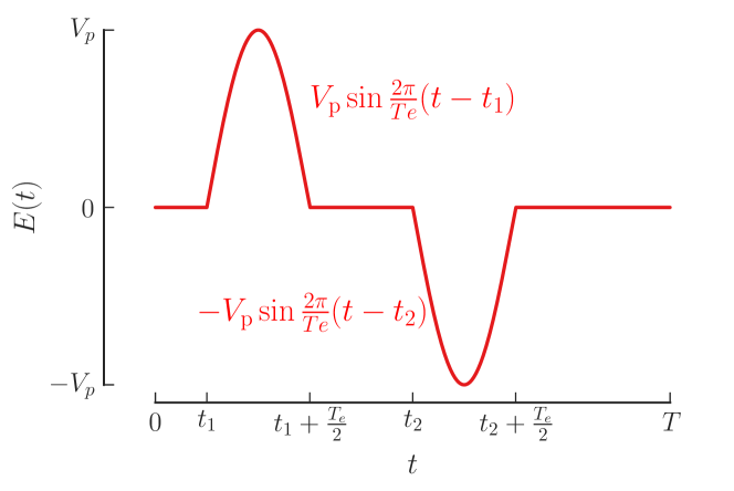
Figure 11: The function $E(t)$ consists of two half-sine lobes, given by Eq. 18, that occur somewhere between $0\leq t\leq T$.

The RMS of $E(t)$ over a period $T$ can be expressed as:

$$e_{\text{RMS}}(V_{\text{p}},T_{e},T)=\sqrt{\frac{T_{e}}{2T}}V_{\text{p}},$$ (19)

The constants $V_{\text{p}}$ and $T_{e}$ can be determined from the open-circuit EMF waveforms determined by FEA, such as those shown in Fig. 9.

Equation 19 can be used to approximate the open-circuit RMS EMF obtained by FEA, shown in Fig. 9. From Fig. 12, it is clear that this approximation is accurate.

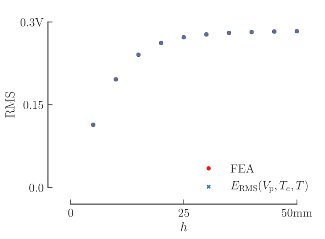
Figure 12: Comparison of Eq. 19 to the RMS of open-circuit EMF simulated using FEA for discrete values of $h$.

Note that Eqs. 19 and 17 both describe the same open circuit RMS EMF, but as functions of different parameters. Since the parameters $V_{\text{p}}$ and $T_{e}$ are dependent on $h$ and if the RMS calculations leading to $e_{\text{RMS}}(h)$ by way of Eq. 17 are performed over the same length of time $T$ used in Eq. 19, then Eqs. 19 and 17 must produce the same RMS value. Hence, for $T=T_{1}$ and $h=h_{1}$,

$$e_{\text{RMS}}(h=h_{1})|_{T=T_{1}}=e_{\text{RMS}}(V_{\text{p}},T_{e},T=T_{1})|_{h=h_{1}}.$$ (20)

3.3.2 Multiple coil, single magnet configuration

We now extend the model for a single-coil single-magnet microgenerator to the more general case of $c$ identical coils, with identical heights $h$, and a single magnet $(m=1)$. As the magnet passes through each of the coils, an EMF of the form shown in Fig. 9 will be induced. This basic waveform will henceforth be referred to as the basic EMF pulse. It has been shown to be well approximated by two half-sine periods.

In addition, we can observe that, for a single-axis microgenerator, as an individual magnet passes through a coil, it induces a basic EMF pulse in that coil. Thus, the number of such pulses $=c\cdot m$, where $c$ is the number of coils and $m$ is the number of magnets present in the system.

Since our goal is to maximize the energy we can harvest, destructive superposition among these sequential pulses should be avoided. For this to occur, two requirements must be met. First, the polarity of the pulses must match. This can be achieved by ensuring the correct sequence of coil polarities. Second, adjacent coils must be spaced in such a way as to optimally superimpose the lobes of successive EMF pulses. This can be achieved by suitable choice of the length and spacing of the coils.

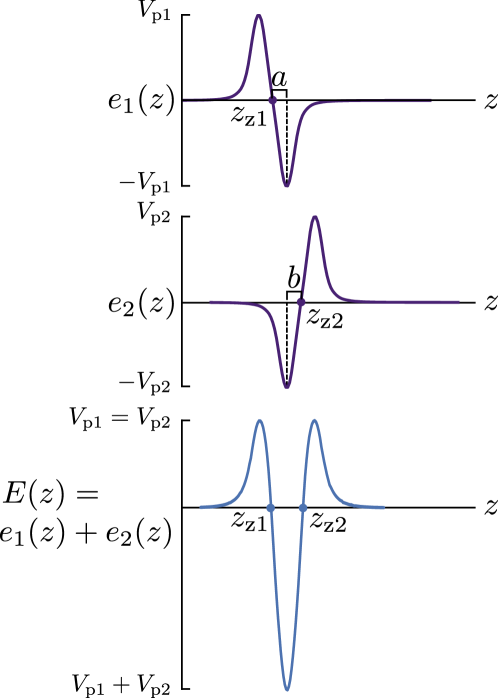
Figure 13: Two individual pulses, $e_{1}(z)$ with peak $V_{\text{p1}}$ and $e_{2}(z)$ with peak $V_{\text{p2}}$, produced by a device with $c=2$ coils and $m=1$ magnet (or alternatively $c=1$, $m=2$ as discussed in Section 3.3.2) and the optimal superposition of the two pulses , resulting in waveform $E(z)$.

Consider the EMF waveform $E(z)$ in Fig. 13, which is the result of a favourable superposition of two successive individual basic EMF pulses $e_{1}(z)$ and $e_{2}(z)$ resulting from the single magnet passing through two successive coils, and where $z$ is the vertical displacement of the magnet. The polarities of the pulses have been matched to ensure that the trailing negative excursion of the first pulse is reinforced by the leading negative extrusion of the second. Since the two coils are identical $V_{\text{p1}}=V_{\text{p2}}$. Furthermore, as can also be seen from Fig. 13, the pulse peaks $V_{\text{p1}}$ and $V_{\text{p2}}$ coincide when the displacement between the zero-crossing (indicated by $z_{\text{z1}}$ and $z_{\text{z2}}$) of the pulses is

$$z_{\text{z2}}-z_{\text{z1}}=a+b,$$ (21)

where $a$ is the $z$-distance between $z_{\text{z1}}$ and the trailing peak of $e_{1}(z)$, and $b$ is the $z$-distance between $z_{\text{z2}}$ and the leading peak of $e_{2}(z)$.

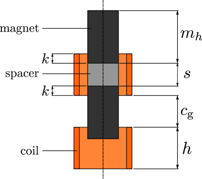
Figure 14: Cross section showing a position of the magnet assembly when it induces one of the EMF waveform peaks. This occurs when the leading or trailing edges of the magnets is a distance $k$ from the edge of the coils. The lengths $m_{\text{h}},s,h$ and $c_{\text{g}}$ denote the magnet height, magnet spacer height, coil height and coil gap, respectively.

The use of the zero-crossings as a frame of reference is deliberate, as their positions are independent of the coil properties and the magnetic field. This is not true for the position of the peaks, for example. The zero-crossings occur when the rate of change of flux $\frac{d\phi}{dt}=0$, which occurs when the centre of the magnet passes through the centre of the coil. Consider Fig. 14, where parameter $k$ indicates the position at which the peaks of a pulse occur and correspond to the displacement between the leading and trailing coil edges and the displacement between leading and trailing magnet edges. This allows Eq. 21 to be related to the dimensions shown in Fig. 14, as follows

$$z_{\text{z2}}-z_{\text{z1}}=c_{\text{g}}+h,$$ (22)

where $c_{\text{g}}$ is the gap between the coils in mm and is given by

$$c_{\text{g}}=m_{\text{h}}-2k.$$ (23)

Since the height $h$ of all coils are identical, Eqs. 22 and 23 will hold for any number of coils when there is a single moving magnet ($m=1$).

Finally, the total internal resistance of the microgenerator $R_{\text{mcrg}}$ is calculated by multiplying the resistance of a single coil $R_{\text{coil}}$, given by Eq. 14, by the number of coils $c$:

$$R_{\text{mcrg}}=c\beta\gamma h.$$ (24)

3.3.3 Single coil, multiple magnet configuration

The previous section extended the model for a single-coil single-magnet microgenerator to one with $c$ identical coils and one magnet ($m=1$). The case of a single coil ($c=1$) and $m$ identical magnets with identical heights $m_{\text{h}}$ can be treated in an analogous way. In this case, the RMS of $E(z)$ is maximized by separating adjacent magnets in the magnet assembly with an iron spacer, and by alternating the polarity of these magnets. As in Section 3.3.2, this leads to opposite polarity for successive pulses. This leads to the requirement:

$$z_{\text{z2}}-z_{\text{z1}}=s+m_{\text{h}},$$ (25)

where $s$ is the spacing between the magnets and $m_{\text{h}}$ is the magnet height. The value of $s$ is given by,

$$s=h-2k,$$ (26)

where once again $k$ can be determined as described on Section 3.3.2.

Since the height of the magnets $m_{\text{h}}$ in the magnet assembly are identical, Eqs. 25 and 26 will hold for any number of magnets.

3.3.4 Multiple coil, multiple magnet configuration

To obtain a model for a microgenerator with $c$ coils and $m$ magnets we simultaneously enforce Eqs. 25 and 22 to obtain:

$$s+m_{\text{h}}=c_{\text{g}}+h.$$ (27)

Now, Eqs. 27, 23 and 26 can be used to determine the spacing of the coils and magnets that optimizes the RMS voltage.

3.3.5 Generalized power delivery by multiple coil, multiple magnet designs

We now consider the peak amplitudes of $E(z)$, the total open-circuit output voltage produced by the linear kinetic energy harvester as an assembly with $m$ magnets that traverses $c$ coils. For ease of analysis, we will normalize these peak voltages by the peak amplitude $V_{\text{p}}$ of the basic pulse, as shown in Fig. 11. The magnitude of these normalized voltages will be denoted by $P(n,c,m)$, where $c$ refers to the number of coils, $m$ the number of magnets and $n$ refers to each peak’s index within the peak sequence. Since all magnets have the same geometry and are evenly spaced, and all coils have the same geometry and are evenly spaced, inspection of Fig. 13 allows us to state for the general case:

For $$m>c$$:

$$P(n,c,m) =\left\{\begin{array}[]{ll}P(-n+\lambda,c,m)&:N_{i}\leq n<0\\ 2c&:0\leq n\leq\lambda\\ 2(m-n)-1&:\lambda<n\leq N_{f}\\ 0&:\text{otherwise,}\end{array}\right.$$ (33)

where

$$\lambda =m-c-1$$

$$N_{f} =m-1$$

$$N_{i} =-c.$$

For $$m=c$$:

$$P(n,c,m) =\left\{\begin{array}[]{ll}P(-n+1,c,m)&:N_{i}\leq n<0\\ 2c-1&:n=0\\ 2(c-n)+1&:0<n\leq N_{f}\\ 0&:\text{otherwise,}\end{array}\right.$$ (39)

where

$$N_{f} =c=m$$

$$N_{i} =c-1=m-1.$$

For $$m<c$$:

$$P(n,c,m) =\left\{\begin{array}[]{ll}P(-n+\lambda,c,m)&:N_{i}\leq n<0\\ 2m&:0\leq n\leq\lambda\\ 2(c-n)-1&:\lambda<n\leq N_{f}\\ 0&:\text{otherwise,}\end{array}\right.$$ (45)

where

$$\lambda =c-m-1$$

$$N_{f} =c-1$$

$$N_{i} =-m.$$

In Eqs. 33, 39 and 45, $N_{i}$ and $N_{f}$ are the values of $n$ that indicate initial and final peak of the peak sequence.

A specific example , for a microgenerator consisting of $c=4$ coils and $m=3$ magnets is shown in Fig. 15. Equations 45, 39 and 33 have been used to calculate the magnitudes of the peaks produced by a microgenerator.

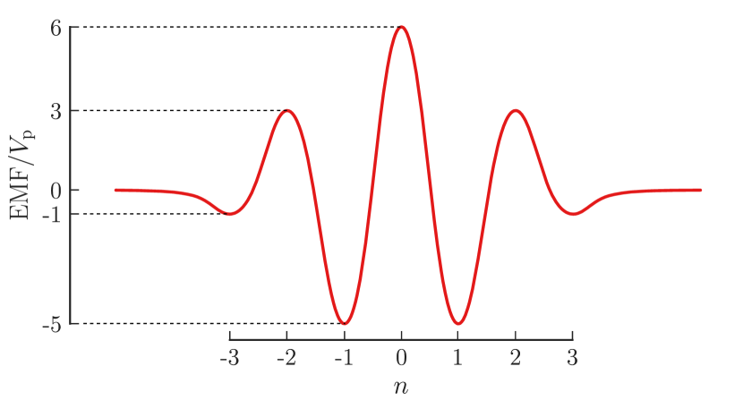
Figure 15: An example, showing the waveform produced by a microgenerator consisting of $c=3$ coils and $m=3$ magnets, for a magnet assembly moving through the coils at a constant velocity. If we use Eq. 45, as for this example $m<c$, we correctly predict the relative magnitude of peaks in the waveform to be $P(n,4,3)=\{1,3,5,6,5,3,1\}$ for each peak position $n\in\{-3,-2,-1,0,1,2,3\}$.

The true peak voltage is given by:

$$\hat{P}(n,c,m)=|V_{\text{p}}|\cdot P(n,c,m).$$ (46)

This allows a comparison between kinetic microgenerators with different magnet and coil properties, and hence different values of $V_{\text{p}}$.

Next we extend Eq. 19, which models the open-circuit RMS voltage as a function of coil height $h$ for a single coil, single magnet configuration, to the general case of $c$ coils and $m$ magnets. Since $E(t)$ consists of a series of half-sine wave lobes, with each lobe’s peak given by Eq. 46, the open-circuit RMS voltage when $c$ coils and $m$ magnets are considered can be obtained by applying Eq. 19:

$$E_{\text{RMS}}(c,m)=\sqrt{\frac{T_{e}}{4T}\sum_{n=N_{i}}^{N_{f}}\hat{P}(n,c,m)^{2}},$$ (47)

where $T_{\text{e}}$ is the period of the basic pulse.

Equation 47 provides an approximation of the final open-circuit RMS voltage delivered by the energy harvester in terms of design parameters $c$ and $m$. However, since $T_{e}$ and $\hat{P}(n,c,m)$ depend on $h$, this result can be developed further. We begin by defining the ratio of RMS open-circuit voltages of microgenerators with different values of $c$ and $m$, but identical $h$ using Eq. 47:

$$\eta(c_{1},m_{1},c_{2},m_{2}) =\frac{E_{\text{RMS}}(c_{2},m_{2})|_{h}}{E_{\text{RMS}}(c_{1},m_{1})|_{h}}$$

$$=\sqrt{\frac{\sum_{N_{i2}}^{N_{f2}}P(n,c_{2},m_{2})^{2}}{\sum_{N_{i1}}^{N_{f1}}P(n,c_{1},m_{1})^{2}}}.$$ (48)

Using Eqs. 17, 19, 20, 48 and 47 and noting, from Eq. 39, that $\sum_{N_{i1}}^{N_{f1}}P(n,1,1)^{2}=1^{2}+1^{2}=2$ and by substituting into Eq. 10, an expression for the average power delivered to the load can be determined:

$$\bar{P}_{\text{load}}(h,c,m,R_{\text{load}})=\frac{A^{2}R_{\text{load}}\cdot(1-\exp(-\alpha h))^{2}\sum_{N_{i}}^{N_{f}}P(n,c,m)^{2}}{2(R_{\text{load}}+R_{\text{mcrg}})^{2}}.$$ (49)

By substituting Eq. 24, the final expression is obtained as a function of all design parameters.

$$\bar{P}_{\text{load}}(h,c,m,R_{\text{load}})=\frac{A^{2}R_{\text{load}}\cdot(1-\exp(-\alpha h))^{2}\sum_{N_{i}}^{N_{f}}P(n,c,m)^{2}}{2(R_{\text{load}}+c\beta\gamma h)^{2}}.$$ (50)

We note again here that Equation 50 is based on an idealized motion in which the magnet assembly moves through the coils at a constant velocity. Hence this result does not necessarily accurately reflect the power that will be produced by the device in practice. It is, however, expected to indicate which microgenerator among competing designs will produce maximum power during practical operation.

We base this assumption on the observation that the magnet assemblies of different microgenerator designs move through the coils with highly similar velocity profiles. Thus, while the result of the predicted power given by Eq. 50 may change for different acceleration impulses and velocities, the ranking of the microgenerator devices based on their expected power output will not. As a result, optimizing for idealized motion can be used as a substitute for optimizing for non-idealized motion in our application.

4 Design application

We now apply the methods presented in the previous section to the design of a microgenerator that harvests the maximum amount of energy from the walking motion of a human test-subject.

4.1 Physical constraints

Due to a strong emphasis on size limitations in our intended eventual application, axially-magnetized cylindrical N35 grade neodymium iron boron (NdFeB) magnets were selected. The magnets have a radius of 5mm and a height of 5mm, and were the strongest readily available at the time. In order to increase the magnetic flux density, two magnets are placed together with poles aligned, resulting in an effective height of 10mm.

Initial experimentation found than an inner tube radius that was 0.5mm greater than the magnet radius ensured unhindered motion of the magnet assembly. The microgenerator tube body was 3D printed using PLA with a thickness of 1mm.

AWG36 gauge copper wire was selected for the coil, giving a wire radius of $r_{c}=0.0635$mm and a resistance per unit length of $R_{\text{gauge}}=1361\times 10^{-6}~{}\Omega/\text{mm}$. The small wire gauge allowed a large winding density close to the magnet assembly while minimizing the coil diameter. The resistance per unit length of the wire was also taken into consideration, as its higher value allows flexibility in load-matching by varying $h$, and hence $R_{\text{mcrg}}$, as per Eq. 24.

The horizontal coil thickness $c_{\text{th}}$ plays a significant role in the open-circuit EMF that is induced. While this does present another possible avenue for optimization, the effect of $c_{\text{th}}$ is currently not explicitly modelled as a parameter. Instead, by selecting a $c_{\text{th}}$ value, its effects will be modelled implicitly in Eq. 17. We determined a suitable value of $c_{\text{th}}$ by FEA, whereby the value of $c_{\text{th}}$ is large enough to provide a turn density $\gamma$ and resistance per turn $\beta$ that allows for increased EMF and load impedance-matching capability by varying the coil height $h$, without resulting in an excessively large internal coil resistance $R_{\text{coil}}$ and severe power losses in the microgenerator. This resulted in a horizontal coil thickness of $c_{\text{th}}=0.725$mm, which serves as a compromise between these two extremes. The bottom thickness of the tube and the thickness of the tube lid was selected as $t_{\text{up}}=t_{\text{lo}}=2$mm.

The maximum vertical space available for the microgenerator is constrained to $L=125$\mathrm{m}\mathrm{m}$$. Using dimensions as defined in Fig. 16, the total height is given by

$$L=2M+C+m_{\text{h}}+m_{\text{f}}+f_{\text{h}}+t_{\text{up}}+t_{\text{lo}}$$ (51)

where

$$M =m\cdot m_{\text{h}}+(m-1)s$$ (52)

$$C =c\cdot h+(c-1)c_{\text{g}}$$ (53)

$$f_{\text{h}} =\delta^{-1}_{\text{mag}}(w_{\text{M}}),$$ (54)

and $w_{\text{M}}$ is the weight of the magnet assembly. An expression for the magnet assembly floating height $f_{\text{h}}$ is obtained by considering the microgenerator at static equilibrium, where the magnetic spring force $\delta_{\text{mag}}(z)$ is equal to the weight of the magnet assembly. As shown in Fig. 16, the floating height is defined the distance between the magnet assembly and the bottom magnet. Using Eq. 54, the floating height $f_{\text{h}}$ can be expressed as:

$$\delta_{\text{mag}}(f_{\text{h}})=w_{\text{M}},$$ (55)

Thus the vertical height is constrained by

$$2M+C+m_{\text{h}}+m_{\text{f}}+f_{\text{h}}+t_{\text{up}}+t_{\text{lo}}\leq 125$\mathrm{m}\mathrm{m}$.$$ (56)

Figure 16: Vertical dimensions of kinetic microgenerator body, showing the required range of motion of the magnet assembly.

For the magnet assembly to move through all the coils, sufficient range of vertical motion is required. This places an additional constraint on the minimum height of the device. The minimum range of relative motion required is

$$z_{\text{m}|\text{t,top}}-z_{\text{m}|\text{t,rest}}\geq M+C+m_{\text{h}},$$ (57)

where $z_{\text{m}|\text{t}}=z_{m}-z_{t}$ as shown in Fig. 16.

Experimentation indicated that the magnet assembly cannot be reliably constructed for a spacer height less than $s<s_{\text{min}}=2.5\text{mm}$. This places an implicit constraint on $h$, which we can derive from Eq. 26,

$$h\geq s_{\text{min}}+2k$$ (58)

Equations 51, 52, 53, 54, 57 and 58 now provide a set of parameterized constraints that can be used to produce a set of optimized microgenerator configurations that conform to the practical limitations of the application.

4.2 Parameter calculation and optimization

We are now in a position to calculate the parameters of the mechanical system model and the parameters of the electrical system model. Using both sets of parameters, full optimization of the microgenerator is performed. This results in a number of possible architectures for subsequent comparison and assessment.

4.2.1 Mechanical system model

For the mechanical system model, the magnetic spring force $\delta_{\text{mag}}(z)$ is found by determining the force between two magnets at discrete points using FEA and then fitting Eq. 7 to these values. For our choice of magnets this results in the following relation for $\delta(z)$, where $z$ is in metres.

$$\delta(z)=\frac{$2.943\text{\times}{10}^{-3}$}{4\pi z^{2}+$1.125\text{\times}{10}^{-4}$},$$ (59)

The footstep acceleration function $a_{\text{step}}(t)$ is determined from measurements taken at the lower leg of a walking human, a sample of which is shown in Fig. 17(a). From video footage, the maximum vertical displacement of the leg was determined to be $s_{\text{h}}=0.15$\mathrm{m}$$ and the upstroke-downstroke delay to be approximately $t_{\text{delay}}=0.05$\mathrm{s}$$. The values of the footstep accelerations, $a_{\text{step}}(t)$, are calculated using Eqs. 2 and 3. The resulting function is shown in Fig. 17(b).

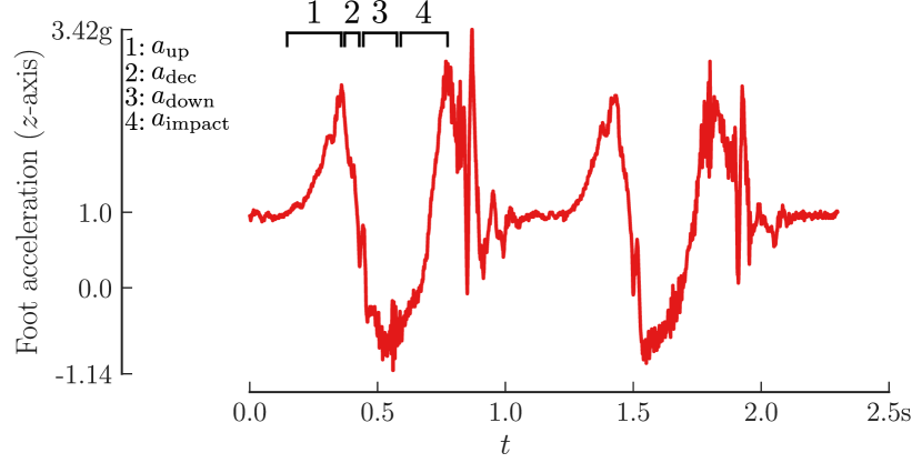
(a)

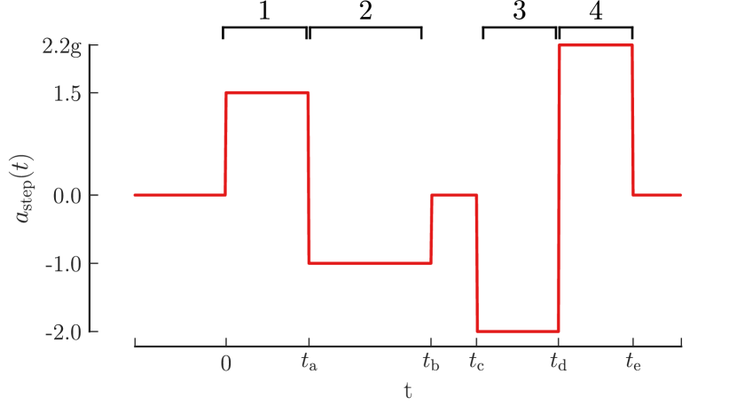
(b)

Figure 17: Comparison of accelerometer measurements from the leg of a human (in the $z$-direction) with artificial footstep described in Section 3. (a) Typical accelerometer measurements from leg of human in the $z$-direction. The foot experiences upward accelerations of approximately 2g, downard accelerations of approximately 2g and impact accelerations of 2.2 to 2.42g, after removing the residual gravity measured by the accelerometer. The footstep stages, described in Fig. 3, are indicated. (b) Artificial footstep used as input for physical system model, with corresponding time instances specified in Table 1. This is a human-specific instance of the general footstep model proposed in Fig. 2.

$t$	seconds
$t_{\text{start}}$	$0$
$t_{\text{a}}$	$0.091$
$t_{\text{b}}$	$0.225$
$t_{\text{c}}$	$0.275$
$t_{\text{d}}$	$0.365$
$t_{\text{e}}$	$0.447$

Table 1: Time intervals corresponding to selected artificial footstep footstep function, shown in Fig. 17(b).

Finally, the damping coefficient $b_{\text{damper}}$ is experimentally determined as

$$b_{\text{damper}}=150\cdot S_{M},$$ (60)

where $S_{\text{M}}$ is the outer surface area of a cylinder, excluding end caps, of the magnet assembly.

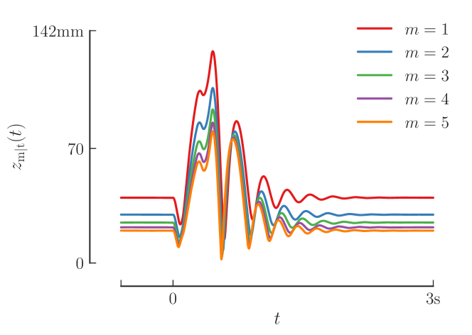
Figure 18: Numerical solution of Eq. 4 for the relative displacement $z_{\mathrm{m|t}}(t)$ between the magnet assembly and the microgenerator tube with input shown in Fig. 17(b) for different number of magnets $m$.

By numerically solving for the parameters of our mechanical system model, given by Eq. 4, the motional constraint given by Eq. 57 can be found for different numbers of magnets $m$. This constraint can then be imposed during architecture optimization. Figure 18 shows the numerical solution of the mechanical system model and indicates the predicted relative displacement between the magnet assembly and the microgenerator tube for different values of $m$.

4.2.2 Electrical system model

The values of $r_{\text{c}}$ and $R_{\text{gauge}}$ were selected in Section 4.1, allowing coil properties $\gamma$ and $\beta$ to be calculated using Eqs. 11 and 13, respectively. In our specific case, this gives

$$\beta \approx 0.059227~{}\Omega\text{/turn}$$ (61)

$$\gamma \approx 40.06~{}\text{turns/mm}.$$ (62)

Recall that Eqs. 11 and 13 are two key coil properties that allow for the coil resistance of the microgenerator $R_{\text{mcrg}}$ to be estimated. As the coil height $h$ and the number of coils $c$ varies during the optimization process, this too leads to variation in $R_{\text{mcrg}}$ during optimization. Since the estimation of the load power is dependent on $R_{\text{mcrg}}$, it must be known at each optimization step. This is made possible by substituting Eqs. 61 and 62 into Eq. 50 during the optimization process.

Next, FEA is used to simulate the EMF pulse of a single-coil, single-magnet model with coil properties given by Eqs. 61 and 62 for a range of discrete values of $h$. The RMS of the EMF is calculated for each pulse that is produced. Equation 17 is subsequently fit to this RMS data, giving an accurate approximation of the open-circuit RMS EMF as a continuous function of $h$,

$$e_{\text{RMS}}(h)\approx 0.2860(1-\exp(-0.1111h)).$$ (63)

FEA is also used to determine the point at which the magnet assembly induces the EMF peaks, denoted with dimension $k$ in Fig. 14. The value of $k$ was found to vary with the coil height $h$ for the range of coil heights tested ($h\leq 50\text{mm}$) with the following relationship:

$$k=h/4.$$ (64)

The final electrical system parameter that must be determined is the electrical load $R_{\text{load}}$. In our case this consists of a full-wave bridge rectifier and a BQ25504 energy harvester from Texas Instruments. Since the dynamic behaviour of this device’s input resistance is not specified, it was measured.

It is expected that the kinetic microgenerator will produce an average waveform pulse current between $5\text{mA}\leq i_{\text{input}}\leq 10\text{mA}$. As a result, the electrical load was selected as $R_{\text{load}}=40\Omega$.

4.3 Architecture optimization

An optimal architecture for the kinetic microgenerator can be determined by maximizing the value of Eq. 50 in terms of the parameters $c,m$ and $h$, given the physical constraints.

Since the number of coils and magnets are integers $c,m\in\mathbb{Z}$, a grid of integer values of $c$ and $m$ are used to search for the optimum solution, with each cell of the grid treated as an independent, restricted optimization problem of Eq. 50, with parameters $c$ and $m$ fixed. In each case, an optimal value of the parameter $h$ is determined using the sequential least squares programming algorithm (SLSQP)[29].

The seven best configurations determined by this procedure and their corresponding parameters are listed in Table 2, alongside a control baseline architecture that consists of a single coil of height $h=10$mm and a single magnet. The control represents a baseline for what would be considered a naive or initial experimental design for a linear kinetic energy harvester, which consists of a single coil and a single magnet where certain design verification is performed using FEA [30], and is typically found in commercially available energy-harvesting shaker flashlights.

Design	$\bar{P}_{\text{load}}$ (W)	$c$	$m$	$h$ (mm)	$L_{\text{min}}$ (mm)
1	$1.988\,99\text{\times}{10}^{-3}$	2	2	$9.72$	124.67
2	$1.379\,92\text{\times}{10}^{-3}$	1	3	$5.98$	125.0
3	$1.172\,82\text{\times}{10}^{-3}$	1	2	$12.97$	115.78
4	$0.627\,19\text{\times}{10}^{-3}$	3	1	$8.34$	114.74
5	$0.6146\text{\times}{10}^{-3}$	4	1	$6.97$	125
6	$0.596\,775\text{\times}{10}^{-3}$	2	1	$9.87$	102.86
7	$0.390\,94\text{\times}{10}^{-3}$	1	1	$12.97$	91.03
Control	$0.3756\text{\times}{10}^{-3}$	1	1	$10.00$	88.06

Table 2: Relative power and design parameters for the set of most optimal kinetic microgenerator designs.

The best design uses $c=2$ coils each with a height of $h=9.72\text{mm}$ in conjunction with a magnet assembly consisting of $m=2$ magnets.

At this point it must be recalled that the power values given by Eq. 50 are based on an idealized motion, in which the magnet assembly moves through the coils with constant velocity. While the power estimate does not necessarily accurately indicate the power that will be produced by the device in practice, it is expected to be indicative of the microgenerator design that will produce maximum power during normal operation. Hence these power figures will only be viewed as a relative measure of power for use in comparison with other potential designs.

The microgenerator configurations in Table 2 were assessed by simulating the top three configurations and the control using FEA for idealized motion, and calculating the power each design would deliver to $R_{\text{load}}$. The results of this comparison are shown in Fig. 19.

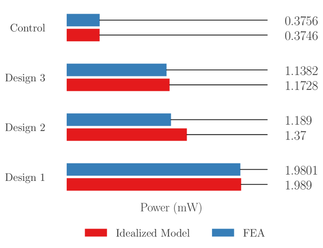
Figure 19: By comparing the results of the proposed model Eq. 50 and the FEA results of $\bar{P}_{\text{load}}$, it is shown that the proposed model produces predictions with a high degree of accuracy.

From Fig. 19 we see that the results produced by the idealized model described by Eq. 50 closely match those of the simulation. It is interesting to note that the proposed model over-estimates the power by a small degree for all configurations other than the control. This is due to the assumption made by the proposed model that the leading and trailing edge of the individual waveforms for the case of $c>1$ and/or $m>1$, as shown in Fig. 13, do not overlap with the lobes of other waveforms. This is an approximation, and the small degree of such overlap that does occur in practice leads to a small degree of destructive interference. This is expected to be more prominent for smaller values of $h$, because in this case there is greater overlap between adjacent pulses. In addition, by treating the pulses as a series of half-sine waveforms, the small EMF present prior to the first pulse and after the last pulse is neglected. However, Fig. 19 indicates that the effect of these factors is small across a diverse set of microgenerator designs.

5 Practical testing

We now experimentally validate our previous assumption that a microgenerator configuration produced by the proposed model and optimized for idealized linear motion remains an optimal microgenerator in practice for more complex motion.

5.1 Methodology

The microgenerator configurations shown in Figure 19 were built and assembled according to their specifications, with only a single exception: the tube height for all configurations was set to $L=125\text{mm}$ to ease the production process. Since the constraint on the tube height is $L_{\text{min}}\leq L\leq 125\text{mm}$, with $L_{\text{min}}$ given for each configuration in Table 2, this has no effect on the test outcome. The assembled microgenerators are shown alongside their magnet assemblies in Figure 20. The assembled generators each have a total mass of 31.592g for Design 1, 32.673g for Design 2, 29.238g for Design 3 and 17.248g for the Control.

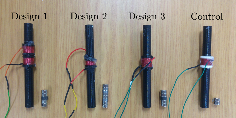
Figure 20: The top three and control microgenerator configurations and magnet assemblies were produced according to the specifications in Section 4.

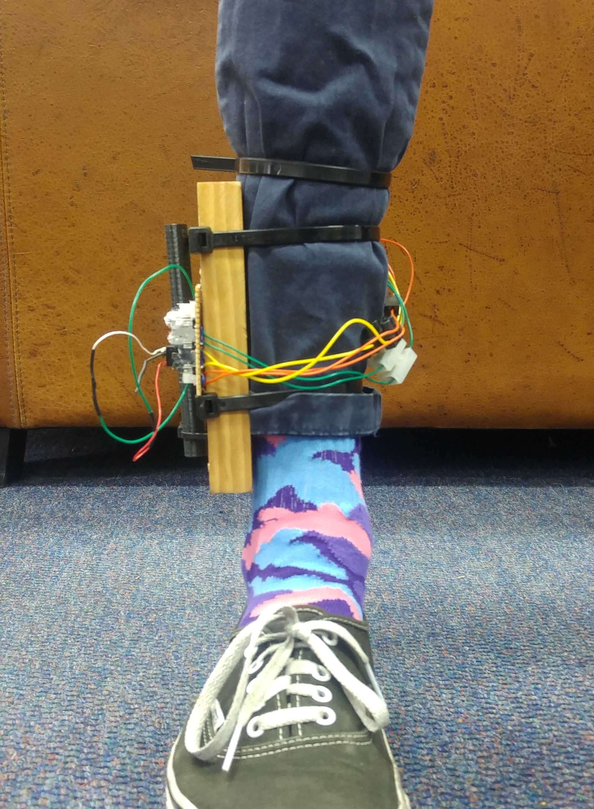
(a) Front view.

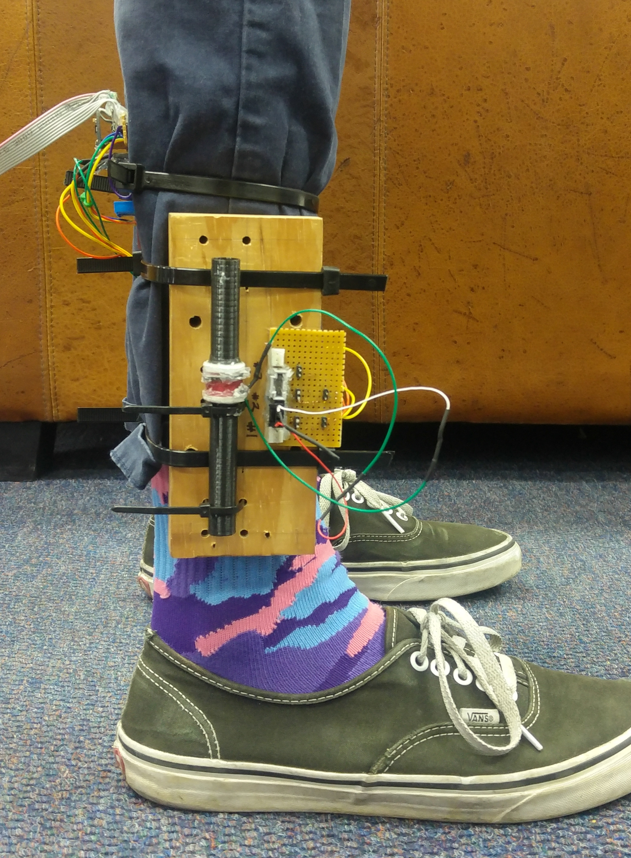
(b) Side view.

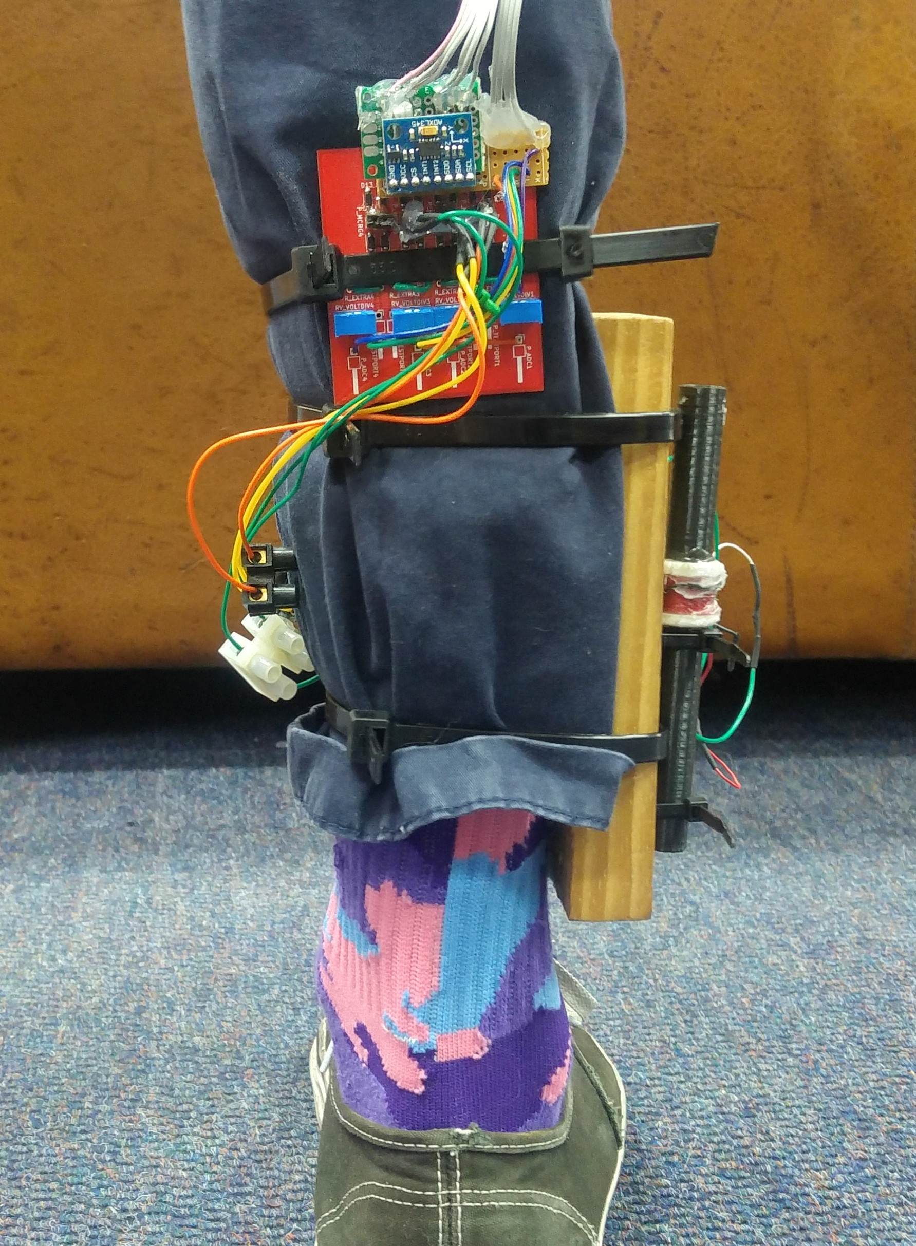
(c) Rear view.

Figure 21: For the human control test a mount that can hold a microgenerator device is attached the outer leg, with the voltage divider and accelerometer attached to the back of the leg.

A mount was fixed to the outer side of a human test subject’s leg as shown in Fig. 21. The mount allows the microgenerator to be easily and quickly swapped between tests, and ensures that it remains vertically aligned. A full-wave bridge rectifier, voltage divider and accelerometer is attached the leg and a data logger is held in-hand. A simplified circuit diagram is shown in Figure 22. The open-circuit EMF that is induced by the microgenerator is rectified, scaled and logged synchronously with the accelerometer output.

Figure 22: Simplified circuit diagram of the electronic circuit used for the test procedure.

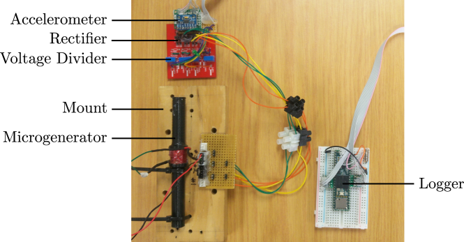
Figure 23: The human control test is performed using a logger, microgenerator mount and an electronic circuit consisting of a full-wave bridge rectifier, voltage divider and accelerometer.

Two sets of practical tests are performed. The first considers the open-circuit case, where no load is attached and the open-circuit EMF is measured. The power that this EMF would deliver to the load can then be calculated using  Eq. 10. The second test considers the closed-circuit case, where a load is attached, and the voltage across this load is measured and used to calculate the power. Hence, the first test evaluates the ideal, open-circuit model for non-idealized motion, while the second test considers the real-world practical case. This allows us to assess first the accuracy of our idealized model, and second our assumption that a microgenerator design that has been optimized using the idealized model remains optimal when applied to the closed-circuit case with a real-world load. Our system load is selected as $R_{\text{load}}=40\Omega$ as discussed in Section 4.2.2.

5.2 Procedure

For each test, the subject walked a predetermined short straight course at a normal pace. The course was approximately 40m in length and perfectly level and clear of obstacles. The course surface consists of concrete surfaced with laminate vinyl flooring. The course took approximately 35 seconds to complete. After each test, the microgenerator was alternated to mitigate the effect of changes in walking speed, style and gait over time. This process is repeated for a total of 160 tests, 40 times for each microgenerator.

5.3 Results

A sample of the measured open-circuit EMF for each microgenerator configuration is shown in Fig. 24. Two pulses are seen for each footstep, the first substantially smaller than the second. The first occurs during the deceleration phase and downward acceleration phase of the footstep, $t_{\text{a}}<t<t_{\text{d}}$ with $t$ as indicated in Fig. 3. The second occurs after impact at $t\geq t_{\text{d}}$, and is followed by some residual EMF induced via oscillation of the magnet assembly on the magnetic spring.

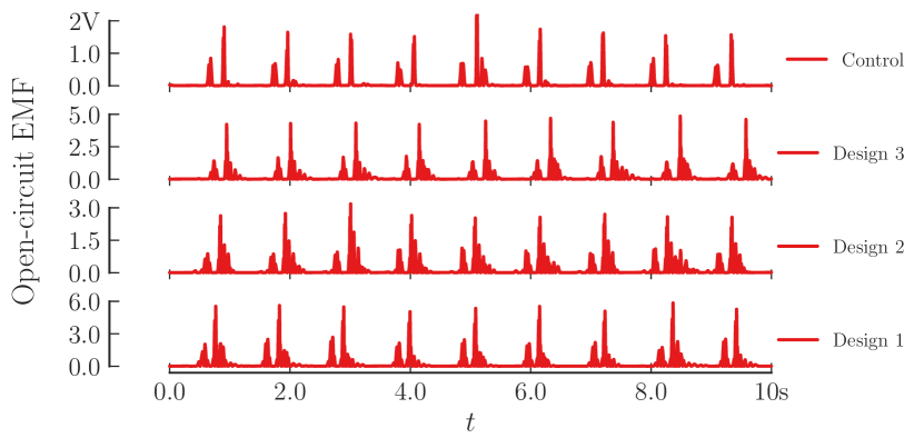
Figure 24: Excerpt from the test measurements of the open-circuit EMF for the microgenerator configurations shown in Fig. 20. A total of 9 footsteps are shown.

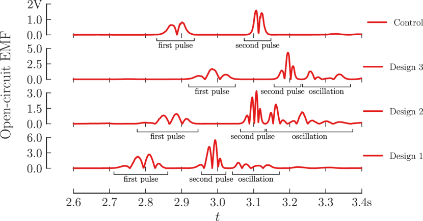
Figure 25: Measured open-circuit EMF for the microgenerator configurations shown in Fig. 20 over an interval corresponding to a single footstep.. The first EMF pulse occurs during the deceleration phase and downward acceleration phase of the footstep and the the second pulse occurs after impact, with the footstep phases shown in Fig. 3. This is followed by an induced EMF due to the oscillation of the magnet assembly.

Figure 25 shows the EMF for a single footstep. As expected, we see that for Design 1 ($c=2,m=2$), Design 2 ($c=1,m=3$) and Design 3 ($c=1,m=2$) and the Control ($c=1,m=1$) there are four, four, three and two peaks respectively. Additional minor peaks can be seen following the two primary pulses as a result of magnet assembly oscillation on the magnetic spring after passing through the coils. It is interesting to note that more EMF is induced from this oscillation for Design 2, which also has the longest magnet assembly ($m=3,s=3\text{mm}$). This allows the upper magnets of the assembly to more easily reach and induce an EMF in the coils. We do not consider this oscillation in the proposed model. However, while not very large, it may provide a means to harvest further energy in future.

The instantaneous power for a series of footsteps for each tested microgenerator configuration for a $R_{\text{load}}=40\Omega$ load is calculated from the open-circuit EMF using Eqs. 9 and 10.

The distribution of the calculated average power dissipated in the load $\bar{P}_{\text{load}}$ for each tested microgenerator configuration calculated using Eq. 10 is illustrated in Fig. 26. It shows that the order of the power generated by the practical microgenerators agrees with the order of the predicated power output shown in Fig. 19. It is also noteworthy that the relative differences between the median of the tested configurations mirrors that in Fig. 19. This provides supporting evidence for our hypothesis that optimization for idealized motion serves as a functional substitute for the optimization for non-idealized motion, as discussed in Section 3.3.5.

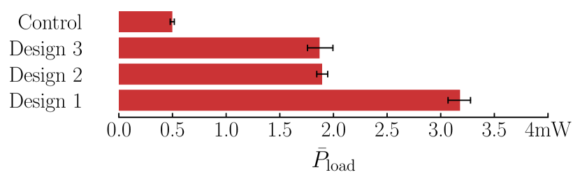
Figure 26: The calculated average power dissipated in a $40\Omega$ load for each tested microgenerator configuration given the measured open-circuit RMS of the EMF. The Design 1, Design 2, Design 3 and Control configurations have a median average power of 3.144mW, 1.886mW, 1.736mW and 0.512mW respectively.

For the closed-circuit case, the distribution of the average power dissipated in the load for each tested microgenerator configuration is shown in Fig. 27. We see that the relative power delivered to the load by each microgenerator agrees with the idealized power output that was presented in Fig. 19. This means that the best microgenerator design in terms of the idealized model remains the best design when attached to a practical load, and hence that the idealized model is suitable for the purpose of optimizing the microgenerator design. Note also that the power output in Fig. 27 is slightly lower than the corresponding open-circuit power shown in Fig. 26. This is due to the electro-mechanical coupling that is present in the closed-circuit case.

The results shown in Figs. 26 and 27 indicate strong supporting evidence for the assumption that the optimization of the microgenerator design when assuming idealized motion serves as a functional substitute for optimization under non-idealized motion, as discussed in Section 3.3.5.

The first design, which delivers median load power of 3.01mW, produces the most power by a large margin. The second and third designs produce similar levels of power (1.856mW and 1.673mW) while the control produces substantially less power with a median of 0.324mW. If we consider the 3.01mW available on average from Device 1 we note that this is likely to be sufficient to power an energy harvesting circuit and one of the many ultra-low power microcontroller units commercially available today. With sufficient power-saving measures, it is quite possible to envision a self-sustaining system powered by energy harvested from the sporadic kinetic motion associated with human or animal footsteps.

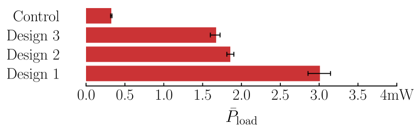
Figure 27: The measured average power dissipated in a $40\Omega$ load for each tested microgenerator configuration. Design 1, Design 2, Design 3 and the Control configuration deliver median average powers of 3.01mW, 1.856mW, 1.673mW and 0.324mW respectively.

By calculating the physical volume occupied by each microgenerator we can calculate the power density of each configuration, measured in $\mu\text{W}/\text{cm}^{3}$, shown in Table 3. There appears to be a strong correspondence between the number of coils and magnets and the power density. This is an expected result given the superposition of subsequent EMF pulses discussed in Section 3.3.5, which allows significant increases in EMF without commensurable increases in device length and, hence, volume.

Design	Median $\bar{P}_{\text{load}}$	Volume ($\text{cm}^{3}$)	Power density ($\mu\text{W}/\text{cm}^{3}$)
1	$3.010$	$16.78$	$179.380$
2	$1.856$	$15.11$	$122.833$
3	$1.673$	$15.72$	$106.425$
4	$0.324$	$15.46$	$20.957$

Table 3: The median average load power dissipated in the load, microgenerator volume and power density of each tested microgenerator configuration.

6 Potential applications

The method we have proposed is applicable to any form of motion that can be modelled as a series of impulsive forces along the z-axis, and not just the footstep-like motion we use to demonstrate effectiveness. Since the formulation explicitly allows the imposition of constraints such as vertical height and cross-section limits, it is well-suited for the design of microgenerators that provide optimal energy generation in size- or weight-constrained situations. Alternatively, it allows a case-by-case assessment of the feasibility of kinetic microgeneration based on the design parameters, load and input forces. The computational model employed eliminates the need for iterative prototyping and practical testing, thereby reducing both the time and the cost of microgenerator design.

The particular application which has motivated this research is wildlife tracking, where size and weight limitations are severe and it is essential to harvest as much power as possible within these constraints. While this remains our first intended practical application, we believe there may be many others. These include energy harvesting from human walking to power wearable technology, and from the impulse-like nature of uneven road surfaces to power autonomous vehicle-mounted sensors.

7 Conclusion

We have considered a linear kinetic energy harvester architecture that consists of an assembly of one or more spaced magnets that passes through one or more coils when the device experiences motion along its axis and that is suspended by a magnetic spring. We considered the specific case of impulsive acceleration as might be the results of a footstep, and not harmonic vibration usually assumed for kinetic energy harvesting. We introduced a mechanical and electrical system model that allows this microgenerator architecture to be optimized for power supplied to a load in terms of its design parameters. These parameters include the individual coil height, number of coils, number of magnets in the magnet assembly and the relative spacing between the coils and magnets. By deliberately designing the model to allow the incorporation of constraints and by selecting a compatible optimization technique, we are able to adapt our architecture to any impulse-like excitation provided there is sufficient single-axis motion.

Our technique was evaluated by application to the practical scenario of designing a microgenerator that can be worn on the leg of a human or animal. First, we predict the top three designs given the physical size constraints. Next, we build physical prototypes of these three designs and measure their performance when attached to the leg of a human subject while walking. In all cases, a baseline system with the simplest possible design is also evaluated. We find that the theoretically predicted relative ordering of the produced power agrees with that observed for the practical systems. This demonstrates that the theoretical optimization also led to practically optimal results. In all cases, the designed system far outperformed the baseline.

The best microgenerator configuration achieved an average load power of 3.144mW, supplied to a $40\Omega$ load giving a power density of 179.380$\mu W/\text{cm}^{3}$ from foot impact accelerations of approximately 2.2g. This firmly places the best micrognerator configuration in the realm of ultra-low power microcontrollers, making powering of such devices a realistic possibility.

8 Acknowledgments

The authors gratefully acknowledge financial support by the National Research Foundation of the Republic of South Africa, by Telkom South Africa, and by Innovus of Stellenbosch University. The authors also gratefully acknowledge the invaluable assistance of Mr Wessel Croukamp in the physical construction of the devices.

9 Funding declaration

We wish to confirm and declare the following sources of funding and/or research grants that were received in the course of study, research or assembly of this work:

• The National Research Foundation (NRF) of South Africa

• Telkom South Africa

• Innovus of Stellenbosch University

The above sponsors have not played any role in the study design; collection; analysis and interpretation of data in the writing of the report; and in the decision to submit the article for publication.

References

- [1] J. M. Conrad, “A survey of energy harvesting sources for embedded systems,” in IEEE SoutheastCon 2008. IEEE, apr 2008, pp. 442–447. [Online]. Available: http://ieeexplore.ieee.org/lpdocs/epic03/wrapper.htm?arnumber=4494336
- [2] R. Vullers, R. van Schaijk, I. Doms, C. Van Hoof, and R. Mertens, “Micropower energy harvesting,” Solid-State Electronics, vol. 53, no. 7, pp. 684–693, jul 2009. [Online]. Available: http://www.sciencedirect.com/science/article/pii/S0038110109000720
- [3] S. Sudevalayam and P. Kulkarni, “Energy Harvesting Sensor Nodes: Survey and Implications,” IEEE Communications Surveys & Tutorials, vol. 13, no. 3, pp. 443–461, 2011. [Online]. Available: http://ieeexplore.ieee.org/lpdocs/epic03/wrapper.htm?arnumber=5522465
- [4] J. M. Gilbert and F. Balouchi, “Comparison of energy harvesting systems for wireless sensor networks,” International Journal of Automation and Computing, vol. 5, no. 4, pp. 334–347, oct 2008. [Online]. Available: http://link.springer.com/10.1007/s11633-008-0334-2
- [5] R. V. Bobryk and D. Yurchenko, “On enhancement of vibration-based energy harvesting by a random parametric excitation,” Journal of Sound and Vibration, vol. 366, pp. 407–417, 2016. [Online]. Available: http://dx.doi.org/10.1016/j.jsv.2015.11.033
- [6] W. Wang, J. Cao, N. Zhang, J. Lin, and W. H. Liao, “Magnetic-spring based energy harvesting from human motions: Design, modeling and experiments,” Energy Conversion and Management, vol. 132, pp. 189–197, 2017. [Online]. Available: http://dx.doi.org/10.1016/j.enconman.2016.11.026
- [7] W. Yang and S. Towfighian, “A hybrid nonlinear vibration energy harvester,” Mechanical Systems and Signal Processing, vol. 90, pp. 317–333, 2017. [Online]. Available: http://dx.doi.org/10.1016/j.ymssp.2016.12.032
- [8] A. Haroun, I. Yamada, and S. Warisawa, “Study of electromagnetic vibration energy harvesting with free/impact motion for low frequency operation,” Journal of Sound and Vibration, vol. 349, pp. 389–402, 2015. [Online]. Available: http://www.sciencedirect.com/science/article/pii/S0022460X15002874
- [9] K. Kecik, A. Mitura, and J. Warminski, “Energy harvesting from a magnetic levitation system,” International Journal of Non-Linear Mechanics, vol. 94, pp. 200–206, sep 2017. [Online]. Available: https://www.sciencedirect.com/science/article/pii/S002074621730241X?via{%}3Dihub
- [10] M. Marszal, B. Witkowski, K. Jankowski, P. Perlikowski, and T. Kapitaniak, “Energy harvesting from pendulum oscillations,” International Journal of Non-Linear Mechanics, vol. 94, no. April, pp. 251–256, 2017.
- [11] M. P. Soares dos Santos, J. A. F. Ferreira, J. A. O. Simões, R. Pascoal, J. Torrão, X. Xue, and E. P. Furlani, “Magnetic levitation-based electromagnetic energy harvesting: a semi-analytical non-linear model for energy transduction,” Scientific Reports, vol. 6, no. 1, p. 18579, may 2016. [Online]. Available: http://www.nature.com/articles/srep18579
- [12] D. F. Berdy, D. J. Valentino, and D. Peroulis, “Kinetic energy harvesting from human walking and running using a magnetic levitation energy harvester,” Sensors and Actuators, A: Physical, vol. 222, pp. 262–271, 2015. [Online]. Available: http://dx.doi.org/10.1016/j.sna.2014.12.006
- [13] C. Serre, A. Pérez-Rodríguez, N. Fondevilla, E. Martincic, S. Martínez, J. R. Morante, J. Montserrat, and J. Esteve, “Design and implementation of mechanical resonators for optimized inertial electromagnetic microgenerators,” Microsystem Technologies, vol. 14, no. 4-5, pp. 653–658, apr 2008. [Online]. Available: http://link.springer.com/10.1007/s00542-007-0494-y
- [14] S.-D. Kwon, J. Park, and K. Law, “Electromagnetic energy harvester with repulsively stacked multilayer magnets for low frequency vibrations,” Smart Materials and Structures, vol. 22, no. 5, p. 055007, may 2013. [Online]. Available: http://stacks.iop.org/0964-1726/22/i=5/a=055007?key=crossref.a2cc56191125641b68f3d636a2068367
- [15] A. M. Wickenheiser and E. Garcia, “Broadband vibration-based energy harvesting improvement through frequency up-conversion by magnetic excitation,” Smart Materials and Structures, vol. 19, no. 6, p. 065020, jun 2010. [Online]. Available: http://stacks.iop.org/0964-1726/19/i=6/a=065020?key=crossref.7c6533acecb40702c342818b6a2f79ee
- [16] K. Ylli, D. Hoffmann, A. Willmann, P. Becker, B. Folkmer, and Y. Manoli, “Energy harvesting from human motion: exploiting swing and shock excitations,” Smart Materials and Structures, vol. 24, no. 2, p. 025029, feb 2015. [Online]. Available: http://stacks.iop.org/0964-1726/24/i=2/a=025029?key=crossref.7f9622e87f20f174a5b5a2dd614d71c7
- [17] C. M. Saravia, J. M. Ramírez, and C. D. Gatti, “A hybrid numerical-analytical approach for modeling levitation based vibration energy harvesters,” Sensors and Actuators, A: Physical, vol. 257, pp. 20–29, 2017. [Online]. Available: http://dx.doi.org/10.1016/j.sna.2017.01.023
- [18] D. Carroll and M. Duffy, “Modelling, design, and testing of an electromagnetic power generator optimized for integration into shoes,” Proceedings of the Institution of Mechanical Engineers, Part I: Journal of Systems and Control Engineering, vol. 226, no. 2, pp. 256–270, feb 2012. [Online]. Available: http://pii.sagepub.com/lookup/doi/10.1177/0959651811411406
- [19] S. P. le Roux, J. Marias, R. Wolhuter, and T. Niesler, “Animal-borne behaviour classification for sheep (Dohne Merino) and Rhinoceros (Ceratotherium simum and Diceros bicornis),” Animal Biotelemetry, vol. 5, no. 1, p. 25, dec 2017. [Online]. Available: https://animalbiotelemetry.biomedcentral.com/articles/10.1186/s40317-017-0140-0
- [20] H. M. Blackie, “Comparative Performance of Three Brands of Lightweight Global Positioning System Collars,” Journal of Wildlife Management, vol. 74, no. 8, pp. 1911–1916, nov 2010. [Online]. Available: http://www.bioone.org/doi/abs/10.2193/2009-412
- [21] M. Hebblewhite, M. Percy, and E. H. Merrill, “Are All Global Positioning System Collars Created Equal? Correcting Habitat-Induced Bias Using Three Brands in the Central Canadian Rockies,” Journal of Wildlife Management, vol. 71, no. 6, pp. 2026–2033, aug 2007. [Online]. Available: http://www.bioone.org/doi/abs/10.2193/2006-238
- [22] M. Masoumi and Y. Wang, “Repulsive magnetic levitation-based ocean wave energy harvester with variable resonance: Modeling, simulation and experiment,” Journal of Sound and Vibration, vol. 381, pp. 192–205, 2016. [Online]. Available: http://dx.doi.org/10.1016/j.jsv.2016.06.024
- [23] G. Donoso, C. L. Ladera, and P. Martín, “Magnet fall inside a conductive pipe: motion and the role of the pipe wall thickness,” Eur. J. Phys. J. Phys, vol. 30, no. 30, pp. 855–855, 2009. [Online]. Available: http://iopscience.iop.org/0143-0807/30/4/018
- [24] T. von Büren and G. Tröster, “Design and optimization of a linear vibration-driven electromagnetic micro-power generator,” Sensors and Actuators A: Physical, vol. 135, no. 2, pp. 765–775, 2007. [Online]. Available: http://www.sciencedirect.com.ez.sun.ac.za/science/article/pii/S0924424706005413
- [25] F. Khan, B. Stoeber, F. Sassani, F. Khan, B. Stoeber, and F. Sassani, “Modeling and simulation of linear and nonlinear MEMS scale electromagnetic energy harvesters for random vibration environments.” TheScientificWorldJournal, vol. 2014, p. 742580, 2014. [Online]. Available: http://www.ncbi.nlm.nih.gov/pubmed/24605063
- [26] P. Zeng and A. Khaligh, “A Permanent-Magnet Linear Motion Driven Kinetic Energy Harvester,” IEEE Transactions on Industrial Electronics, vol. 60, no. 12, pp. 5737–5746, dec 2013. [Online]. Available: http://ieeexplore.ieee.org/document/6359913/
- [27] D. Vokoun, M. Beleggia, L. Heller, and P. Šittner, “Magnetostatic interactions and forces between cylindrical permanent magnets,” Journal of Magnetism and Magnetic Materials, vol. 321, no. 22, pp. 3758–3763, 2009.
- [28] B. P. Mann and N. D. Sims, “Energy harvesting from the nonlinear oscillations of magnetic levitation,” Journal of Sound and Vibration, vol. 319, no. 1-2, pp. 515–530, 2009.
- [29] D. Kraft, “A software package for sequential quadratic programming,” Institute for Flight Mechanics, Koln, Germany, Tech. Rep., 1988.
- [30] V. Bedekar, J. Oliver, and S. Priya, “Pen harvester for powering a pulse rate sensor,” Journal of Physics D: Applied Physics, vol. 42, no. 10, p. 105105, may 2009. [Online]. Available: http://stacks.iop.org/0022-3727/42/i=10/a=105105?key=crossref.6e3dc42c217b694ce465a1ab208f2f8a