Analysis and approximation of a vorticity-velocity-pressure formulation for the Oseen equations

Abstract

We introduce a family of mixed methods and discontinuous Galerkin discretisations designed to numerically solve the Oseen equations written in terms of velocity, vorticity, and Bernoulli pressure. The unique solvability of the continuous problem is addressed by invoking a global inf-sup property in an adequate abstract setting for non-symmetric systems. The proposed finite element schemes, which produce exactly divergence-free discrete velocities, are shown to be well-defined and optimal convergence rates are derived in suitable norms. In addition, we establish optimal rates of convergence for a class of discontinuous Galerkin schemes, which employ stabilisation. A set of numerical examples serves to illustrate salient features of these methods.

Key words: Oseen equations; vorticity-based formulation; mixed finite elements; exactly divergence-free velocity; discontinuous Galerkin schemes; numerical fluxes; a priori error bounds.

Mathematics subject classifications (2000): 65N30, 65N12, 76D07, 65N15.

1 Introduction

The Oseen equations stem from linearisation of the steady (or alternatively from the backward Euler time-discretisation of the transient) Navier-Stokes equations. Of particular appeal to us is their formulation in terms of fluid velocity, vorticity vector, and pressure. A diversity of discretisation methods is available to solve incompressible flow problems using these three fields as principal unknowns. Some recent examples include spectral elements [3, 8] as well as stabilised and least-squares schemes [2, 9] for Navier-Stokes; also several mixed and augmented methods for Brinkman [4, 5, 7], and a number of other discretisations specifically designed for Stokes flows [6, 22, 23, 25, 30].

Both the implementation and the analysis of numerical schemes for Navier-Stokes are typically based on the Oseen linearisation. A few related contributions (not only restricted to the velocity-pressure formulation) include for instance [10], that presents a least-squares method for Navier-Stokes equations with vorticity-based first-order reformulation, and whose analysis exploits the elliptic theory of Agmon- Douglas-Nirenberg. Conforming finite element methods exhibit optimal order of accuracy for diverse boundary conditions. We also mention the non-conforming exponentially accurate least-squares spectral method for Oseen equations proposed in [27], where a suitable preconditioner is also proposed. In [32] the authors introduce a velocity-vorticity-pressure least-squares finite element method for Oseen and Navier-Stokes equations with velocity boundary conditions. They derive error estimates and reported a degeneracy of the convergence for large Reynolds numbers. A div least-squares minimisation problem based on the stress-velocity-pressure formulation was introduced in [13]. The study shows that the corresponding homogeneous least-squares functional is elliptic and continuous in suitable norms. Several first-order Oseen-type systems are analysed in [15], also including vorticity and total pressure in the formulation.

Discontinuous Galerkin (DG) methods have also been used to solve the Oseen problem, as for example, in [19, 18] for the case of Dirichlet boundary conditions. Compared with conforming finite elements, discretisations based on DG methods have a number of attractive, and well-documented features. These include high order accuracy, being amenable for $hp$-adaptivity, relatively simple implementation on highly unstructured meshes, and superior robustness when handling rough coefficients. We also mention the a priori error analysis of hybridisable DG schemes introduced in [16] for the Oseen equations. The family of DG methods we propose here has resemblance with those schemes, but exploits a three-field formulation described below.

This paper is concerned with mixed non-symmetric variational problems which will be analysed using a global inf-sup argument. To do this, we conveniently restrict the set of equations to the space of divergence-free velocities, and apply results from [24] in order to prove that the equivalent resulting non-symmetric saddle-point problem is well-posed. For the numerical approximation, we first consider Raviart-Thomas elements of order $k\geq 0$ for the velocity field, Nédélec elements or order $k$ for the vorticity, and piecewise polynomials of degree $k$ without continuity restrictions, for the Bernoulli pressure. We prove unique solvability of the discrete problem by adapting the same tools utilised in the analysis of the continuous problem. In addition, the proposed family of Galerkin finite element methods turns out to be optimally convergent, under the common assumptions of enough regularity of the exact solutions to the continuous problem. The method produces exactly divergence-free approximations of the velocity by construction; thus preserving, at the discrete level, an essential constraint of the governing equations. Next, inspired by the methods presented in [20, 19], we present another scheme involving the discontinuous Galerkin discretisation of the $\mathop{\mathbf{curl}}\nolimits$-$\mathop{\mathbf{curl}}\nolimits$ and $\mathrm{grad}$-$\mathrm{div}$ operators. We prove the well-posedness of the DG scheme and derive error estimates under some solution regularity assumptions.

We have structured the contents of the paper in the following manner. Notation-related preliminaries are stated in the remainder of this Section. We then present the model problem as well as the three-field weak formulation and its solvability analysis in Section 2. The finite element discretisation is constructed in Section 3, where we also derive the stability and convergence bounds. In Section 4, we present the mixed DG formulation for the model problem. The well-posedness of the method and the error analysis are established in the same section. We close in Section 5 with a set of numerical tests that illustrate the properties of the proposed numerical schemes in a variety of scenarios.

Let $\Omega$ be a bounded domain of $\mathbb{R}^{3}$ with Lipschitz boundary $\partial\Omega$. Moreover, we assume that $\partial\Omega$ admits a disjoint partition $\partial\Omega=\Gamma\cup\Sigma$. For any $s\geq 0$, the symbol $\left\|\cdot\right\|_{s,\Omega}$ denotes the norm of the Hilbertian Sobolev spaces $\mathrm{H}^{s}(\Omega)$ or $\mathrm{H}^{s}(\Omega)^{3}$, with the usual convention $\mathrm{H}^{0}(\Omega):=\mathrm{L}^{2}(\Omega)$. For $s\geq 0$, we recall the definition of the space

$$\mathrm{H}^{s}(\mathop{\mathbf{curl}}\nolimits;\Omega):=\left\{\boldsymbol{\theta}\in\mathrm{H}^{s}(\Omega)^{3}:\ \mathop{\mathbf{curl}}\nolimits\boldsymbol{\theta}\in\mathrm{H}^{s}(\Omega)^{3}\right\},$$

endowed with the norm $\left\|\boldsymbol{\theta}\right\|^{2}_{\mathrm{H}^{s}(\mathop{\mathbf{curl}}\nolimits;\Omega)}=\left\|\boldsymbol{\theta}\right\|_{s,\Omega}^{2}+\left\|\mathop{\mathbf{curl}}\nolimits\boldsymbol{\theta}\right\|^{2}_{s,\Omega}$, and will denote $\mathrm{H}(\mathop{\mathbf{curl}}\nolimits;\Omega)=\mathrm{H}^{0}(\mathop{\mathbf{curl}}\nolimits;\Omega)$. Finally, $c$ and $C$, with subscripts, tildes, or hats, will represent a generic constant independent of the mesh parameter $h$.

2 Statement and solvability of the continuous problem

Oseen problem in terms of velocity-vorticity-pressure.

A standard backward Euler time-discretisation of the classical Navier-Stokes equations, or a linearisation of the steady version of the problem combined with standard curl-div identities, leads to the following set of equations, known as the Oseen equations (see [29, 26]):

$$\begin{split}\sigma\boldsymbol{u}-\nu\Delta\boldsymbol{u}+\mathop{\mathbf{curl}}\nolimits\boldsymbol{u}\times\boldsymbol{\beta}+\nabla p&=\boldsymbol{f}\qquad\mbox{ in }\Omega,\\ \mathop{\mathrm{div}}\nolimits\boldsymbol{u}&=0\qquad\,\mbox{ in }\Omega,\end{split}$$ (2.1)

where $\nu>0$ is the kinematic fluid viscosity, $\sigma>0$ is inversely proportional to the time-step, $\boldsymbol{\beta}$ is an adequate approximation of velocity to be made precise below, and the vector of external forces $\boldsymbol{f}$ also absorbs the contributions related to previous time steps, or to fixed states in the linearisation procedure of the steady Navier-Stokes equations. As usual in this context, in the momentum equation we have conveniently introduced the Bernoulli (also known as dynamic) pressure $p:=P+\frac{1}{2}|\boldsymbol{u}|^{2}$, where $P$ is the actual fluid pressure.

The structure of (2.1) suggests to introduce the rescaled vorticity vector $\boldsymbol{\omega}:=\sqrt{\nu}\mathop{\mathbf{curl}}\nolimits\boldsymbol{u}$ as a new unknown. Furthermore, in this study we focus on the case of zero normal velocities and zero tangential vorticity trace imposed on a part of the boundary $\Gamma\subset\partial\Omega$, whereas a non-homogeneous tangential velocity $\boldsymbol{u}_{\Sigma}$ and a fixed Bernoulli pressure $p_{\Sigma}$ are set on the remainder of the boundary $\Sigma=\partial\Omega\setminus\Gamma$. Therefore, system (2.1) can be recast in the form

$$\sigma\boldsymbol{u}+\sqrt{\nu}\mathop{\mathbf{curl}}\nolimits\boldsymbol{\omega}+\nu^{-1/2}\boldsymbol{\omega}\times\boldsymbol{\beta}+\nabla p=\boldsymbol{f},\quad\boldsymbol{\omega}-\sqrt{\nu}\mathop{\mathbf{curl}}\nolimits\boldsymbol{u}=\boldsymbol{0},\quad\text{and}\quad\mathop{\mathrm{div}}\nolimits\boldsymbol{u} =0 \mbox{ in }\Omega,$$

$$\boldsymbol{u}\cdot\boldsymbol{n}=0\quad\text{ and }\quad\boldsymbol{\omega}\times\boldsymbol{n} =\boldsymbol{0} \mbox{ on }\Gamma,$$ (2.2)

$$p=p_{\Sigma}\quad\text{ and }\quad\boldsymbol{u}\times\boldsymbol{n} =\boldsymbol{u}_{\Sigma} \mbox{ on }\Sigma,$$

where $\boldsymbol{n}$ stands for the outward unit normal on $\partial\Omega$. Should the boundary $\Sigma$ have zero measure, the additional condition $(p,1)_{\Omega,0}=0$ is required to enforce uniqueness of the Bernoulli pressure.

Defining a weak formulation.

Let us introduce the following functional spaces

$$\mathrm{H}:=\{\boldsymbol{v}\in\mathrm{H}(\mathop{\mathrm{div}}\nolimits;\Omega):\boldsymbol{v}\cdot\boldsymbol{n}=0\,\,\text{on}\,\,\Gamma\},\quad\mathrm{Z}:=\{\boldsymbol{\theta}\in\mathrm{H}(\mathop{\mathbf{curl}}\nolimits;\Omega):\gamma_{t}(\boldsymbol{\theta})=\boldsymbol{0}\,\,\text{on}\,\,\Gamma\},\quad\text{and }\quad\mathrm{Q}:=\mathrm{L}^{2}(\Omega),$$

where the operator $\gamma_{t}$ is the tangential trace operator on $\Gamma$, defined by: $\gamma_{t}(\boldsymbol{\theta})=\boldsymbol{\theta}\times\boldsymbol{n}$. Let us endow $\mathrm{H}$ and $\mathrm{Q}$ with their natural norms. For the space $\mathrm{Z}$ however, we consider the following viscosity-weighted norm:

$$\|\boldsymbol{\theta}\|_{\mathrm{Z}}:=\left(\|\boldsymbol{\theta}\|_{0,\Omega}^{2}+\nu\|\mathop{\mathbf{curl}}\nolimits\boldsymbol{\theta}\|_{0,\Omega}^{2}\right)^{1/2}.$$

From now on, we will assume that the data are regular enough: $\boldsymbol{\beta}\in\mathrm{L}^{\infty}(\Omega)^{3}$ and $\boldsymbol{f}\in\mathrm{L}^{2}(\Omega)^{3}$. We proceed to test (2.2) against adequate functions and to impose the boundary conditions in such a manner that we end up with the following formulation: Find $(\boldsymbol{u},\boldsymbol{\omega},p)\in\mathrm{H}\times\mathrm{Z}\times\mathrm{Q}$ such that

$$a(\boldsymbol{u},\boldsymbol{v}) + \;b_{1}(\boldsymbol{v},\boldsymbol{\omega}) +b_{2}(\boldsymbol{v},p)+c(\boldsymbol{\omega},\boldsymbol{v}) =\;F(\boldsymbol{v}) \qquad\forall\boldsymbol{v}\in\mathrm{H},$$

$$b_{1}(\boldsymbol{u},\boldsymbol{\theta}) - \;d(\boldsymbol{\omega},\boldsymbol{\theta}) =\;G(\boldsymbol{\theta}) \qquad\forall\boldsymbol{\theta}\in\mathrm{Z},$$ (2.3)

$$b_{2}(\boldsymbol{u},q) =\;0 \qquad\forall q\in\mathrm{Q},$$

where the bilinear forms $a:\mathrm{H}\times\mathrm{H}\to\mathbb{R}$, $b_{1}:\mathrm{H}\times\mathrm{Z}\to\mathbb{R}$, $d:\mathrm{Z}\times\mathrm{Z}\to\mathbb{R}$, $b_{2}:\mathrm{H}\times\mathrm{Q}\to\mathbb{R}$, $c:\mathrm{Z}\times\mathrm{H}\to\mathbb{R}$, and the linear functionals $F:\mathrm{H}\to\mathbb{R}$, and $G:\mathrm{Z}\to\mathbb{R}$ are specified as follows

$$a(\boldsymbol{u},\boldsymbol{v}) :=\sigma\int_{\Omega}\boldsymbol{u}\cdot\boldsymbol{v}\,d\boldsymbol{x},\quad b_{1}(\boldsymbol{v},\boldsymbol{\theta}):=\sqrt{\nu}\int_{\Omega}\mathop{\mathbf{curl}}\nolimits\boldsymbol{\theta}\cdot\boldsymbol{v}\,d\boldsymbol{x},\quad b_{2}(\boldsymbol{v},q):=-\int_{\Omega}q\mathop{\mathrm{div}}\nolimits\boldsymbol{v}\,d\boldsymbol{x},$$

$$d(\boldsymbol{\omega},\boldsymbol{\theta}) :=\int_{\Omega}\boldsymbol{\omega}\cdot\boldsymbol{\theta}\,d\boldsymbol{x},\quad c(\boldsymbol{\theta},\boldsymbol{v}):=\frac{1}{\sqrt{\nu}}\int_{\Omega}(\boldsymbol{\theta}\times\boldsymbol{\beta})\cdot\boldsymbol{v}\,d\boldsymbol{x},$$

$$F(\boldsymbol{v}) :=\int_{\Omega}\boldsymbol{f}\cdot\boldsymbol{v}\,d\boldsymbol{x}-\langle\boldsymbol{v}\cdot\boldsymbol{n},p_{\Sigma}\rangle_{\Sigma},\quad G(\boldsymbol{\theta}):=-\sqrt{\nu}\langle\boldsymbol{u}_{\Sigma},\boldsymbol{\theta}\rangle_{\Sigma},$$

for all $\boldsymbol{u},\boldsymbol{v}\in\mathrm{H}$, $\boldsymbol{\omega},\boldsymbol{\theta}\in\mathrm{Z}$, and $q\in\mathrm{Q}$.

Solvability analysis.

In order to analyse the variational formulation (2.3), let us introduce the Kernel of the bilinear form $b_{2}(\cdot,\cdot)$ and its classical characterisation

$$\mathrm{X}:=\{\boldsymbol{v}\in\mathrm{H}\,:\,b_{2}(\boldsymbol{v},q)=0,\quad\forall\,q\in Q\}\,=\,\{\boldsymbol{v}\in\mathrm{H}\,:\,\mathop{\mathrm{div}}\nolimits\boldsymbol{v}\,=\,0\;\;\text{in}\;\;\Omega\},$$

and let us recall that $b_{2}$ satisfies the inf-sup condition:

$$\sup_{\stackrel{{\scriptstyle\scriptstyle\boldsymbol{v}\in\mathrm{H}}}{{\boldsymbol{v}\neq 0}}}\frac{|b_{2}(\boldsymbol{v},q)|}{\|\boldsymbol{v}\|_{\mathrm{H}}}\geq\beta_{2}\|q\|_{0,\Omega}\quad\forall q\in\mathrm{Q},$$ (2.4)

with an inf-sup constant $\beta_{2}>0$ only depending on $\Omega$ (see e.g. [24]).

We will now address the well-posedness of (2.3). To that end, it is enough to study its reduced counterpart, defined on $\mathrm{X}\times\mathrm{Z}$: Find $(\boldsymbol{u},\boldsymbol{\omega})\in\mathrm{X}\times\mathrm{Z}$ such that

$$a(\boldsymbol{u},\boldsymbol{v}) + \;b_{1}(\boldsymbol{v},\boldsymbol{\omega}) +c(\boldsymbol{\omega},\boldsymbol{v}) =\;F(\boldsymbol{v}) \qquad\forall\boldsymbol{v}\in\mathrm{X},$$

$$b_{1}(\boldsymbol{u},\boldsymbol{\theta}) - \;d(\boldsymbol{\omega},\boldsymbol{\theta}) =\;G(\boldsymbol{\theta}) \qquad\forall\boldsymbol{\theta}\in\mathrm{Z}.$$ (2.5)

The equivalence between (2.3) and (2.5) is established in the following result, whose proof follows [26] and it is basically a direct consequence of the inf-sup condition (2.4).

Lemma 2.1

If $(\boldsymbol{u},\boldsymbol{\omega},p)\in\mathrm{H}\times\mathrm{Z}\times\mathrm{Q}$ is a solution of (2.3), then $\boldsymbol{u}\in\mathrm{X}$ and $(\boldsymbol{u},\boldsymbol{\omega})\in\mathrm{X}\times\mathrm{Z}$ also solves (2.5). Conversely, if $(\boldsymbol{u},\boldsymbol{\omega})\in\mathrm{X}\times\mathrm{Z}$ is a solution of (2.5), then there exists a unique $p\in\mathrm{Q}$ such that $(\boldsymbol{u},\boldsymbol{\omega},p)\in\mathrm{H}\times\mathrm{Z}\times\mathrm{Q}$ solves (2.3).

The abstract setting that will permit the analysis of (2.3) is stated in the following general result [24, Theorem 1.2].

Theorem 2.1

Let $\mathcal{A}:\mathcal{X}\times\mathcal{X}\to\mathbb{R}$ be a bounded bilinear form and $\mathcal{G}:\mathcal{X}\to\mathbb{R}$ a bounded functional, both defined on the Hilbert space $(\mathcal{X},\langle\cdot,\cdot\rangle_{\mathcal{X}})$. If there exists $\alpha>0$ such that

$$\,\sup_{\scriptstyle y\in{\mathcal{X}}\setminus\{0\}}\frac{\mathcal{A}(x,y)}{\|y\|_{\mathcal{X}}}\,\geq\,\alpha\,\|x\|_{\mathcal{X}}\quad\forall\,x\in\mathcal{X},$$ (2.6)

and

$$\,\sup_{\stackrel{{\scriptstyle\scriptstyle x\in{\mathcal{X}}}}{{y\neq 0}}}\mathcal{A}(x,y)\,>\,0\quad\forall\,y\in\mathcal{X},$$ (2.7)

then there exists a unique solution $x\in\mathcal{X}$ to the problem

$$\mathcal{A}(x,y)=\mathcal{G}(y)\quad\forall\,y\in\mathcal{X}.$$

Furthermore, there exists $C>0$ (independent of $x$) such that

$$\|x\|_{\mathcal{X}}\leq\frac{1}{\alpha}\|\mathcal{G}\|_{\mathcal{X}^{\prime}}.$$

Lemma 2.2

Let us assume that

$$\frac{2\|\boldsymbol{\beta}\|_{\infty,\Omega}^{2}}{\nu\sigma}<1,$$ (2.8)

and let us define the bilinear form $\mathcal{A}(\cdot,\cdot)$ specified as

$$\mathcal{A}((\boldsymbol{u},\boldsymbol{\omega}),(\boldsymbol{v},\boldsymbol{\theta})):=a(\boldsymbol{u},\boldsymbol{v})+\;b_{1}(\boldsymbol{v},\boldsymbol{\omega})+b_{1}(\boldsymbol{u},\boldsymbol{\theta})-\;d(\boldsymbol{\omega},\boldsymbol{\theta})+c(\boldsymbol{\omega},\boldsymbol{v}).$$

Then, there exist $\alpha_{1},\alpha_{2}>0$ such that

$$|\mathcal{A}((\boldsymbol{u},\boldsymbol{\omega}),(\boldsymbol{v},\boldsymbol{\theta}))|\leq\alpha_{1}\|(\boldsymbol{u},\boldsymbol{\omega})\|_{\mathcal{X}}\|(\boldsymbol{v},\boldsymbol{\theta})\|_{\mathcal{X}},$$ (2.9)

and

$$\,\sup_{\stackrel{{\scriptstyle\scriptstyle(\boldsymbol{v},\boldsymbol{\theta})\in{\mathcal{X}}}}{{(\boldsymbol{v},\boldsymbol{\theta})\neq 0}}}\frac{\mathcal{A}((\boldsymbol{u},\boldsymbol{\omega}),(\boldsymbol{v},\boldsymbol{\theta}))}{\|(\boldsymbol{v},\boldsymbol{\theta})\|_{\mathcal{X}}}\,\geq\,\alpha_{2}\,\|(\boldsymbol{u},\boldsymbol{\omega})\|_{\mathcal{X}}\quad\forall\,(\boldsymbol{u},\boldsymbol{\omega})\in\mathcal{X},$$ (2.10)

where $\mathcal{X}:=\mathrm{X}\times\mathrm{Z}$, endowed with the corresponding product norm, is a Hilbert space.

Proof. As a consequence of the boundedness of $a(\cdot,\cdot)$ $b_{1}(\cdot,\cdot)$, $c(\cdot,\cdot)$, and $d(\cdot,\cdot)$, the bilinear form $\mathcal{A}(\cdot,\cdot)$ is bounded and so condition (2.9) readily follows.

Concerning the satisfaction of the inf-sup condition (2.10), for a given $(\boldsymbol{u},\boldsymbol{\omega})\in\mathcal{X}$, we can define

$$\tilde{\boldsymbol{\theta}}:=-\boldsymbol{\omega}\in\mathrm{Z},\quad\text{and}\quad\tilde{\boldsymbol{v}}:=(\boldsymbol{u}+\hat{c}\sqrt{\nu}\mathop{\mathbf{curl}}\nolimits\boldsymbol{\omega})\in\mathrm{X},$$

where $\hat{c}>0$ is a constant to be chosen later. We can then immediately assert that

$$\mathcal{A}((\boldsymbol{u},\boldsymbol{\omega}),(\tilde{\boldsymbol{v}},\tilde{\boldsymbol{\theta}})) =\sigma\int_{\Omega}\boldsymbol{u}\cdot\tilde{\boldsymbol{v}}\,d\boldsymbol{x}+\sqrt{\nu}\int_{\Omega}\mathop{\mathbf{curl}}\nolimits\boldsymbol{\omega}\cdot\tilde{\boldsymbol{v}}\,d\boldsymbol{x}+\sqrt{\nu}\int_{\Omega}\mathop{\mathbf{curl}}\nolimits\tilde{\boldsymbol{\theta}}\cdot\boldsymbol{u}\,d\boldsymbol{x}$$

$$\quad-\int_{\Omega}\boldsymbol{\omega}\cdot\tilde{\boldsymbol{\theta}}\,d\boldsymbol{x}+\frac{1}{\sqrt{\nu}}\int_{\Omega}(\boldsymbol{\omega}\times\boldsymbol{\beta})\cdot\tilde{\boldsymbol{v}}\,d\boldsymbol{x}$$

$$\geq\sigma\|\boldsymbol{u}\|_{0,\Omega}^{2}+\hat{c}\sqrt{\nu}\sigma\int_{\Omega}\boldsymbol{u}\cdot\mathop{\mathbf{curl}}\nolimits\boldsymbol{\omega}\,d\boldsymbol{x}+\sqrt{\nu}\int_{\Omega}\boldsymbol{u}\cdot\mathop{\mathbf{curl}}\nolimits\boldsymbol{\omega}\,d\boldsymbol{x}+\hat{c}\nu\|\mathop{\mathbf{curl}}\nolimits\boldsymbol{\omega}\|_{0,\Omega}^{2}$$

$$\quad-\sqrt{\nu}\int_{\Omega}\boldsymbol{u}\cdot\mathop{\mathbf{curl}}\nolimits\boldsymbol{\omega}\,d\boldsymbol{x}+\|\boldsymbol{\omega}\|_{0,\Omega}^{2}+\frac{1}{\sqrt{\nu}}\int_{\Omega}(\boldsymbol{\omega}\times\boldsymbol{\beta})\cdot\boldsymbol{u}\,d\boldsymbol{x}+\hat{c}\int_{\Omega}(\boldsymbol{\omega}\times\boldsymbol{\beta})\cdot\mathop{\mathbf{curl}}\nolimits\boldsymbol{\omega}\,d\boldsymbol{x}$$

$$\geq\sigma\|\boldsymbol{u}\|_{0,\Omega}^{2}-\frac{\sigma}{4}\|\boldsymbol{u}\|_{0,\Omega}^{2}-\hat{c}^{2}\sigma\nu\|\mathop{\mathbf{curl}}\nolimits\boldsymbol{\omega}\|_{0,\Omega}^{2}+\hat{c}\nu\|\mathop{\mathbf{curl}}\nolimits\boldsymbol{\omega}\|_{0,\Omega}^{2}+\|\boldsymbol{\omega}\|_{0,\Omega}^{2}-\frac{2\sigma}{3}\|\boldsymbol{u}\|_{0,\Omega}^{2}$$

$$\quad-\frac{3\|\boldsymbol{\beta}\|_{\infty,\Omega}^{2}}{2\nu\sigma}\|\boldsymbol{\omega}\|_{0,\Omega}^{2}-\frac{\|\boldsymbol{\beta}\|_{\infty,\Omega}^{2}}{2\nu\sigma}\|\boldsymbol{\omega}\|_{0,\Omega}^{2}-2\hat{c}^{2}\sigma\nu\|\mathop{\mathbf{curl}}\nolimits\boldsymbol{\omega}\|_{0,\Omega}^{2}$$

$$=\frac{\sigma}{12}\|\boldsymbol{u}\|_{0,\Omega}^{2}+\hat{c}\left(1-3\hat{c}\sigma\right)\nu\|\mathop{\mathbf{curl}}\nolimits\boldsymbol{\omega}\|_{0,\Omega}^{2}+\left(1-\frac{2\|\boldsymbol{\beta}\|_{\infty,\Omega}^{2}}{\nu\sigma}\right)\|\boldsymbol{\omega}\|_{0,\Omega}^{2},$$

where we have used the bound $\|\boldsymbol{\omega}\times\boldsymbol{\beta}\|_{0,\Omega}\leq 2\|\boldsymbol{\beta}\|_{\infty,\Omega}\|\boldsymbol{\omega}\|_{0,\Omega}$. Choosing $\hat{c}=1/(4\sigma)$ and exploiting (2.8), we arrive at

$$\mathcal{A}((\boldsymbol{u},\boldsymbol{\omega}),(\tilde{\boldsymbol{v}},\tilde{\boldsymbol{\theta}}))\geq C\|(\boldsymbol{u},\boldsymbol{\omega})\|_{\mathcal{X}}^{2},$$

with $C$ independent of $\nu$. On the other hand, by construction we realise that $\|{\tilde{\boldsymbol{\theta}}}\|_{\mathrm{Z}}=\|\boldsymbol{\omega}\|_{\mathrm{Z}}$ and $\|\tilde{\boldsymbol{v}}\|_{0,\Omega}\leq C\hat{c}(\|\boldsymbol{u}\|_{0,\Omega}+\|\boldsymbol{\omega}\|_{\mathrm{Z}})$, and consequently

$$\sup_{\stackrel{{\scriptstyle\scriptstyle(\boldsymbol{v},\boldsymbol{\theta})\in\mathcal{X}}}{{(\boldsymbol{v},\boldsymbol{\theta})\neq 0}}}\frac{\mathcal{A}((\boldsymbol{u},\boldsymbol{\omega}),(\boldsymbol{v},\boldsymbol{\theta}))}{\|(\boldsymbol{v},\boldsymbol{\theta})\|_{\mathcal{X}}}\geq\frac{\mathcal{A}((\boldsymbol{u},\boldsymbol{\omega}),(\tilde{\boldsymbol{v}},\tilde{\boldsymbol{\theta}}))}{\|(\tilde{\boldsymbol{v}},\tilde{\boldsymbol{\theta}})\|_{\mathcal{X}}}\geq\alpha_{2}\|(\boldsymbol{u},\boldsymbol{\omega})\|_{\mathcal{X}}\qquad\forall(\boldsymbol{u},\boldsymbol{\omega})\in\mathcal{X},$$

which finishes the proof. $\square$

Lemma 2.3

Suppose that the bound (2.8) is satisfied. Then, there exists $C>0$ such that

$$\,\sup_{\stackrel{{\scriptstyle\scriptstyle(\boldsymbol{u},\boldsymbol{\omega})\in{\mathcal{X}}}}{{(\boldsymbol{u},\boldsymbol{\omega})\neq(0,0)}}}\mathcal{A}((\boldsymbol{u},\boldsymbol{\omega}),(\boldsymbol{v},\boldsymbol{\theta}))\,>\,0\quad\forall\,(\boldsymbol{v},\boldsymbol{\theta})\in\mathcal{X}.$$

Proof. For all $(\boldsymbol{v},\boldsymbol{\theta})\in\mathcal{X}$, we have that:

$$\mathcal{A}((\boldsymbol{v},-\boldsymbol{\theta}),(\boldsymbol{v},\boldsymbol{\theta})) =\sigma\|\boldsymbol{v}\|_{0,\Omega}^{2}+\|\boldsymbol{\theta}\|_{0,\Omega}^{2}-\frac{1}{\sqrt{\nu}}\int_{\Omega}(\boldsymbol{\theta}\times\boldsymbol{\beta})\cdot\boldsymbol{v}\,d\boldsymbol{x}$$

$$\geq\sigma\|\boldsymbol{v}\|_{0,\Omega}^{2}+\|\boldsymbol{\theta}\|_{0,\Omega}^{2}-\frac{\sigma}{2}\|\boldsymbol{v}\|_{0,\Omega}^{2}-\frac{2\|\boldsymbol{\beta}\|_{\infty,\Omega}^{2}}{\nu\sigma}\|\boldsymbol{\theta}\|_{0,\Omega}^{2}$$

$$\geq\frac{\sigma}{2}\|\boldsymbol{v}\|_{0,\Omega}^{2}+\left(1-\frac{2\|\boldsymbol{\beta}\|_{\infty,\Omega}^{2}}{\nu\sigma}\right)\|\boldsymbol{\theta}\|_{0,\Omega}^{2}.$$

$\square$

As a consequence of the previous lemmas, we have the following result.

Theorem 2.2

Let us assume (2.8). Then, the variational problem (2.5) admits a unique solution $(\boldsymbol{u},\boldsymbol{\omega})\in\mathrm{X}\times\mathrm{Z}$. Moreover, there exists $C>0$ such that

$$\|\boldsymbol{u}\|_{\mathrm{H}}+\|\boldsymbol{\omega}\|_{\mathrm{Z}}\leq C(\|\boldsymbol{f}\|_{0,\Omega}+\|p_{\Sigma}\|_{1/2,\Sigma}+\|\boldsymbol{u}_{\Sigma}\|_{-1/2,\Sigma}).$$ (2.11)

Proof. It suffices to verify the hypotheses of Theorem 2.1. First, we define the linear functional

$$\mathcal{G}(\boldsymbol{v},\boldsymbol{\theta}):=F(\boldsymbol{v})+G(\boldsymbol{\theta}),$$

which is bounded on $\mathrm{X}\times\mathrm{Z}$. Thus, the proof follows from Lemmas 2.2 and 2.3. $\square$

The following result establishes the corresponding stability estimate for the Bernoulli pressure.

Corollary 1

Let $(\boldsymbol{u},\boldsymbol{\omega})\in\mathrm{X}\times\mathrm{Z}$, be the unique solution of (2.5), with $\boldsymbol{u}$ and $\boldsymbol{\omega}$ satisfying (2.11). In addition, let $p\in Q$ be the unique pressure provided by Lemma 2.1, so that $(\boldsymbol{u},\boldsymbol{\omega},p)\in\mathrm{H}\times\mathrm{Z}\times\mathrm{Q}$ is the unique solution of (2.3). Then, there exists $C>0$ such that

$$\|p\|_{0,\Omega}\leq C(\|\boldsymbol{f}\|_{0,\Omega}+\|p_{\Sigma}\|_{1/2,\Sigma}+\|\boldsymbol{u}_{\Sigma}\|_{-1/2,\Sigma}).$$

Proof. Combining the inf-sup condition (2.4) with the first equation in (2.3) gives the bound

$$\|p\|_{0,\Omega}\leq\frac{1}{\beta_{2}}\sup_{\stackrel{{\scriptstyle\scriptstyle\boldsymbol{v}\in\mathrm{H}}}{{\boldsymbol{v}\neq 0}}}\frac{|b_{2}(\boldsymbol{v},p)|}{\|\boldsymbol{v}\|_{\mathrm{H}}}=\frac{1}{\beta_{2}}\sup_{\stackrel{{\scriptstyle\scriptstyle\boldsymbol{v}\in\mathrm{H}}}{{\boldsymbol{v}\neq 0}}}\frac{|F(\boldsymbol{v})-a(\boldsymbol{u},\boldsymbol{v})-b_{1}(\boldsymbol{v},\boldsymbol{\omega})-c(\boldsymbol{\omega},\boldsymbol{v})|}{\|\boldsymbol{v}\|_{\mathrm{H}}},$$

which together with (2.11), and the boundedness of $F$, $a$, $b_{1}$ and $c$, complete the proof. $\square$

Remark 2.1

An alternative analysis for the nonsymmetric variational problem (2.3) can be carried out using a fixed-point argument that allows a symmetrisation of the mixed structure. The resulting weak form could then be analysed using classical tools for saddle-point problems, for instance, following the similar treatment in [14]. Establishing inf-sup conditions for the off-diagonal bilinear forms in the original nonsymmetric formulation is, however, much more involved (see e.g. [28]).

Remark 2.2

Assumption (2.8) holds provided one chooses $\sigma$ appropriately. As this parameter represents the inverse of the timestep, the aforementioned relation constitutes then a CFL-type condition. We also note that this bound for $\boldsymbol{\beta}$ coincides with the hypotheses that yield solvability of least-squares formulations for the Oseen problem analysed in [15, 13].

3 Finite element discretisation

In this section we introduce a Galerkin scheme for (2.3) and analyse its well-posedness by establishing suitable assumptions on the finite element subspaces involved. Error estimates are also derived.

Defining the discrete problem.

Let $\{\mathcal{T}_{h}(\Omega)\}_{h>0}$ be a shape-regular family of partitions of the polyhedral region $\bar{\Omega}$, by tetrahedrons $T$ of diameter $h_{T}$, with mesh size $h:=\max\{h_{T}:\;T\in\mathcal{T}_{h}(\Omega)\}$. In what follows, given an integer $k\geq 0$ and a subset $S$ of $\mathbb{R}^{3}$, $\mathcal{P}_{k}(S)$ will denote the space of polynomial functions defined locally in $S$ and being of total degree $\leq k$.

Moreover, for any $T\in\mathcal{T}_{h}(\Omega)$, we introduce the local Nédélec space

$$\mathbb{N}_{k}(T):=\mathcal{P}_{k}(T)^{3}\oplus R_{k+1}(T),$$

where $R_{k+1}(T)$ is a subspace of $\mathcal{P}_{k+1}(T)^{3}$ composed by homogeneous polynomials of degree $k+1$, and being orthogonal to $\boldsymbol{x}$. With these tools, let us define the following finite element subspaces:

$$\mathrm{Z}_{h} :=\{\boldsymbol{\theta}_{h}\in\mathrm{Z}:\boldsymbol{\theta}_{h}|_{T}\in\mathbb{N}_{k}(T)\quad\forall T\in\mathcal{T}_{h}(\Omega)\},$$ (3.1)

$$\mathrm{Q}_{h} :=\{q_{h}\in\mathrm{Q}:q_{h}|_{T}\in\mathcal{P}_{k}(T)\quad\forall T\in\mathcal{T}_{h}(\Omega)\},$$ (3.2)

$$\mathrm{H}_{h} :=\{\boldsymbol{v}_{h}\in\mathrm{H}:\boldsymbol{v}_{h}|_{T}\in RT_{k}(T)\quad\forall T\in\mathcal{T}_{h}(\Omega)\},$$ (3.3)

where $RT_{k}(T)=\mathcal{P}_{k}(T)^{3}\oplus\mathcal{P}_{k}(T)\boldsymbol{x}$ is the Raviart-Thomas space defined locally in $T\in\mathcal{T}_{h}(\Omega)$.

The proposed Galerkin scheme approximating (2.3) reads as follows: Find $(\boldsymbol{u}_{h},\boldsymbol{\omega}_{h},p_{h})\in\mathrm{H}_{h}\times\mathrm{Z}_{h}\times\mathrm{Q}_{h}$ such that

$$a(\boldsymbol{u}_{h},\boldsymbol{v}_{h}) + \;b_{1}(\boldsymbol{v}_{h},\boldsymbol{\omega}_{h}) +\;b_{2}(\boldsymbol{v}_{h},p_{h})+\;c(\boldsymbol{\omega}_{h},\boldsymbol{v}_{h}) =\;F(\boldsymbol{v}_{h}) \qquad\forall\boldsymbol{v}_{h}\in\mathrm{H}_{h},$$

$$b_{1}(\boldsymbol{u}_{h},\boldsymbol{\theta}_{h}) - \;d(\boldsymbol{\omega}_{h},\boldsymbol{\theta}_{h}) =\;G(\boldsymbol{\theta}_{h}) \qquad\forall\boldsymbol{\theta}_{h}\in\mathrm{Z}_{h},$$ (3.4)

$$b_{2}(\boldsymbol{u}_{h},q_{h}) =\;0 \qquad\forall q_{h}\in\mathrm{Q}_{h}.$$

Solvability and stability of the discrete problem.

The analysis of the Galerkin formulation will follow the same arguments exploited in the continuous setting. Let us then consider the discrete kernel of $b_{2}$:

$$\mathrm{X}_{h}:=\{\boldsymbol{v}_{h}\in\mathrm{H}_{h}\,:\,b_{2}(\boldsymbol{v}_{h},q_{h})=0,\quad\forall\,q\in\mathrm{Q}_{h}\}=\{\boldsymbol{v}_{h}\in\mathrm{H}_{h}\,:\,\mathop{\mathrm{div}}\nolimits\boldsymbol{v}_{h}\equiv 0\quad{\rm in}\quad\Omega\},$$ (3.5)

where the characterisation is indeed possible thanks to the inclusion $\mathop{\mathrm{div}}\nolimits\mathrm{H}_{h}\subseteq\mathrm{Q}_{h}$. Moreover, it is well-known that the following discrete inf-sup condition holds (see [24]):

$$\sup_{\stackrel{{\scriptstyle\scriptstyle\boldsymbol{v}_{h}\in\mathrm{H}_{h}}}{{\boldsymbol{v}_{h}\neq 0}}}\frac{b_{2}(\boldsymbol{v}_{h},q_{h})}{\|\boldsymbol{v}_{h}\|_{\mathrm{H}}}\geq\tilde{\beta}_{2}\|q_{h}\|_{0,\Omega}\quad\forall q_{h}\in\mathrm{Q}_{h}.$$ (3.6)

We again resort to a reduced version of the problem, now defined on the product space $\mathrm{X}_{h}\times\mathrm{Z}_{h}$. Find $(\boldsymbol{u}_{h},\boldsymbol{\omega}_{h})\in\mathrm{X}_{h}\times\mathrm{Z}_{h}$ such that

$$a(\boldsymbol{u}_{h},\boldsymbol{v}_{h}) + \;b_{1}(\boldsymbol{v}_{h},\boldsymbol{\omega}_{h})+\;c(\boldsymbol{\omega}_{h},\boldsymbol{v}_{h})\, =\; F(\boldsymbol{v}_{h})\, \qquad\forall\,\boldsymbol{v}_{h}\in\mathrm{X}_{h},$$

$$b_{1}(\boldsymbol{u}_{h},\boldsymbol{\theta}_{h}) - \;d(\boldsymbol{\omega}_{h},\boldsymbol{\theta}_{h})\, =\; G(\boldsymbol{\theta}_{h})\, \qquad\forall\,\boldsymbol{\theta}_{h}\in\mathrm{Z}_{h},$$ (3.7)

and its equivalence with (3.4) is once more a direct consequence of the inf-sup condition (3.6).

Lemma 3.1

If $(\boldsymbol{u}_{h},\boldsymbol{\omega}_{h},p_{h})\in\mathrm{H}_{h}\times\mathrm{Z}_{h}\times\mathrm{Q}_{h}$ is a solution of (3.4), then $\boldsymbol{u}_{h}\in\mathrm{X}_{h}$, and $(\boldsymbol{u}_{h},\boldsymbol{\omega}_{h})\in\mathrm{X}_{h}\times\mathrm{Z}_{h}$ is also a solution of (3.7). Conversely, if $(\boldsymbol{u}_{h},\boldsymbol{\omega}_{h})\in\mathrm{X}_{h}\times\mathrm{Z}_{h}$ is a solution of (3.7), then there exists a unique $p_{h}\in\mathrm{Q}_{h}$ such that $(\boldsymbol{u}_{h},\boldsymbol{\omega}_{h},p_{h})\in\mathrm{H}_{h}\times\mathrm{Z}_{h}\times\mathrm{Q}_{h}$ is a solution of (3.4).

In order to establish the well-posedness of (3.7), we will employ the following discrete version of Theorem 2.1.

Theorem 3.1

Assume (2.8). Let $k\geq 0$ be an integer and let $\mathrm{X}_{h}$ and $\mathrm{Z}_{h}$ be given by (3.5) and (3.1), respectively. Then, there exists a unique $(\boldsymbol{u}_{h},\boldsymbol{\omega}_{h})\in\mathrm{X}_{h}\times\mathrm{Z}_{h}$ solution of the discrete scheme (3.7). Moreover, there exist positive constants $\hat{C}_{1},\,\hat{C}_{2}>0$ independent of $h$ such that

$$\|\boldsymbol{u}_{h}\|_{\mathrm{H}}+\|\boldsymbol{\omega}_{h}\|_{\mathrm{Z}}\leq\hat{C}_{1}(\|\boldsymbol{f}\|_{0,\Omega}+\|p_{\Sigma}\|_{1/2,\Sigma}+\|\boldsymbol{u}_{\Sigma}\|_{-1/2,\Sigma}),$$ (3.8)

and

$$\|\boldsymbol{u}-\boldsymbol{u}_{h}\|_{\mathrm{H}}+\|\boldsymbol{\omega}-\boldsymbol{\omega}_{h}\|_{\mathrm{Z}}\leq\hat{C}_{2}\inf_{(\boldsymbol{v}_{h},\boldsymbol{\theta}_{h})\in\mathrm{X}_{h}\times\mathrm{Z}_{h}}(\|\boldsymbol{u}-\boldsymbol{v}_{h}\|_{\mathrm{H}}+\|\boldsymbol{\omega}-\boldsymbol{\theta}_{h}\|_{\mathrm{Z}}),$$ (3.9)

where $(\boldsymbol{u},\boldsymbol{\omega})\in\mathrm{X}\times\mathrm{Z}$ is the unique solution to (2.5).

Proof. Let us define $\mathcal{X}_{h}:=\mathrm{X}_{h}\times\mathrm{Z}_{h}$ and reuse the forms $\mathcal{A}(\cdot,\cdot)$ and $\mathcal{G}(\cdot)$ as in the proof of Lemma 2.2. The next step consists in proving that $\mathcal{A}(\cdot,\cdot)$ satisfies the discrete version of the inf-sup conditions (2.6)-(2.7), as in Lemmas 2.2 and  2.3. In order to assert (2.6), we consider $(\boldsymbol{u}_{h},\boldsymbol{\omega}_{h})\in\mathcal{X}_{h}$, and define

$$\tilde{\boldsymbol{\theta}}_{h}:=-\boldsymbol{\omega}_{h}\in\mathrm{Z}_{h},\qquad\text{and }\tilde{\boldsymbol{v}}_{h}:=(\boldsymbol{u}_{h}+\frac{\sqrt{\nu}}{4\sigma}\mathop{\mathbf{curl}}\nolimits\boldsymbol{\omega}_{h})\in\mathrm{X}_{h}.$$

Then, repeating exactly the same steps used in the proof of Lemma 2.2 the discrete version of (2.6) follows. Regarding the discrete version of (2.7), we once again repeat the same arguments given in the proof of Lemma 2.3. Finally, the Céa estimate follows from classical arguments. $\square$

We now state the stability and an adequate approximation property of the discrete pressure.

Corollary 2

Let $(\boldsymbol{u}_{h},\boldsymbol{\omega}_{h})\in\mathrm{X}_{h}\times\mathrm{Z}_{h}$ be the unique solution of (3.7), with $\boldsymbol{u}_{h}$ and $\boldsymbol{\omega}_{h}$ satisfying (3.8). In addition, let $p_{h}\in Q_{h}$ be the unique discrete Bernoulli pressure provided by Lemma 3.1, so that $(\boldsymbol{u}_{h},\boldsymbol{\omega}_{h},p_{h})\in\mathrm{H}_{h}\times\mathrm{Z}_{h}\times\mathrm{Q}_{h}$ is the unique solution of (3.4). Then, there exist positive constants $\bar{C}_{1},\,\bar{C}_{2}>0$, independent of $h$ and $\nu$, such that

$$\|p_{h}\|_{0,\Omega}\leq\bar{C}_{1}(\|\boldsymbol{f}\|_{0,\Omega}+\|p_{\Sigma}\|_{1/2,\Sigma}+\|\boldsymbol{u}_{\Sigma}\|_{-1/2,\Sigma}),$$

and

$$\|p-p_{h}\|_{0,\Omega}\leq\bar{C}_{2}\inf_{(\boldsymbol{v}_{h},\boldsymbol{\theta}_{h},q_{h})\in\mathrm{H}_{h}\times\mathrm{Z}_{h}\times Q_{h}}(\|\boldsymbol{u}-\boldsymbol{v}_{h}\|_{\mathrm{H}}+\|\boldsymbol{\omega}-\boldsymbol{\theta}_{h}\|_{\mathrm{Z}}+\|p-q_{h}\|_{0,\Omega}).$$ (3.10)

Proof. The result follows using the same arguments considered in the proof of Corollary 1, but using the discrete inf-sup condition (3.6). We omit further details. $\square$

A priori error estimates.

Let us introduce for a given $s>1/2$, the Nédeléc global interpolation operator ${\mathcal{R}}_{h}:\mathrm{H}^{s}(\mathop{\mathbf{curl}}\nolimits;\Omega)\cap\mathrm{Z}\to\mathrm{Z}_{h}$. From [1] we known that for all $\boldsymbol{\theta}\in\mathrm{H}^{s}(\mathop{\mathbf{curl}}\nolimits;\Omega)$ with $s>1/2$, there exists $C>0$ independent of $h$, such that

$$\|\boldsymbol{\theta}-{\mathcal{R}}_{h}\boldsymbol{\theta}\|_{\mathrm{Z}}\leq Ch^{\min\{s,k+1\}}\|\boldsymbol{\theta}\|_{\mathrm{H}^{s}(\mathop{\mathbf{curl}}\nolimits;\Omega)}.$$ (3.11)

On the other hand, for the Raviart-Thomas interpolation $\Pi_{h}:\mathrm{H}^{s}(\Omega)^{3}\cap\mathrm{H}\to\mathrm{H}_{h}$, with $s>0$, we recall (see e.g. [24]) that there exists $C>0$, independent of $h$, such that for all $s>0$:

$$\|\boldsymbol{v}-\Pi_{h}\boldsymbol{v}\|_{\mathrm{H}}\leq Ch^{\min\{s,k+1\}}\|\boldsymbol{v}\|_{\mathrm{H}^{s}(\mathop{\mathrm{div}}\nolimits;\Omega)}\quad\forall\boldsymbol{v}\in\mathrm{H}^{s}(\mathop{\mathrm{div}}\nolimits;\Omega)\cap\mathrm{H}.$$ (3.12)

Finally we recall that the orthogonal projection from $\mathrm{L}^{2}(\Omega)$ onto the finite element subspace $\mathrm{Q}_{h}$, here denoted ${\mathcal{P}}_{h}$, satisfies the following error estimate for all $s>0$:

$$\|q-{\mathcal{P}}_{h}q\|_{0,\Omega}\leq Ch^{\min\{s,k+1\}}\|q\|_{s,\Omega}\quad\forall q\in\mathrm{H}^{s}(\Omega).$$ (3.13)

These operators fulfil the following commuting diagram

$$\mathop{\mathrm{div}}\nolimits{\mathcal{R}}_{h}\boldsymbol{v}={\mathcal{P}}_{h}(\mathop{\mathrm{div}}\nolimits\boldsymbol{v})\quad\forall\boldsymbol{v}\in\mathrm{H}^{s}(\Omega)^{3}\cap{\mathrm{H}(\mathrm{div};\Omega)}.$$

The following result summarises the error analysis for our mixed finite element scheme (3.4).

Theorem 3.2

Let $k\geq 0$ be an integer and let $\mathrm{H}_{h},\mathrm{Z}_{h}$ and $\mathrm{Q}_{h}$ be given by (3.1), (3.2), and (3.3). Let $(\boldsymbol{u},\boldsymbol{\omega},p)\in\mathrm{H}\times\mathrm{Z}\times\mathrm{Q}$ and $(\boldsymbol{u}_{h},\boldsymbol{\omega}_{h},p_{h})\in\mathrm{H}_{h}\times\mathrm{Z}_{h}\times\mathrm{Q}_{h}$ be the unique solutions to the continuous and discrete problems (2.3) and (3.4), respectively. Assume that $\boldsymbol{u}\in\mathrm{H}^{s}(\Omega)^{3}$, $\mathop{\mathrm{div}}\nolimits\boldsymbol{u}\in\mathrm{H}^{s}(\Omega)$, $\boldsymbol{\omega}\in\mathrm{H}^{1+s}(\Omega)^{3}$ and $p\in\mathrm{H}^{s}(\Omega)$, for some $s>1/2$. Then, there exists $\hat{C}>0$ independent of $h$ such that

$${\|\boldsymbol{u}-\boldsymbol{u}_{h}\|_{\mathrm{H}}+\|\boldsymbol{\omega}-\boldsymbol{\omega}_{h}\|_{\mathrm{Z}}+\|p-p_{h}\|_{0,\Omega}\leq\hat{C}h^{\min\{s,k+1\}}(\|\boldsymbol{u}\|_{\mathrm{H}^{s}(\mathop{\mathrm{div}}\nolimits;\Omega)}+\|\boldsymbol{\omega}\|_{\mathrm{H}^{s}(\mathop{\mathbf{curl}}\nolimits;\Omega)}+\|p\|_{s,\Omega}).}$$

Proof. The proof follows from (3.9), (3.10), and standard interpolation estimates satisfied by the operators ${\mathcal{R}}_{h}$, $\Pi_{h}$ and ${\mathcal{P}}_{h}$ (see (3.11), (3.12) and (3.13), respectively). $\square$

4 Discontinuous Galerkin method

In this section, we propose and analyse a DG method for (2.2). We provide solvability and stability of the discrete scheme by introducing suitable numerical fluxes. A priori error estimates are also derived.

Preliminaries.

Apart from the definitions laid out at the beginning of Section 3, let us denote by ${\mathcal{E}}_{h}$ the set of internal faces, by ${\mathcal{F}}_{h}^{\Sigma}$ the set of external faces on $\Sigma$ and by ${\mathcal{F}}_{h}^{\Gamma}$ the set of external faces on $\Gamma$. We set ${\mathcal{F}}_{h}={\mathcal{E}}_{h}\cup{\mathcal{F}}_{h}^{\Sigma}\cup{\mathcal{F}}_{h}^{\Gamma}$. We denote by $h_{e}$ the diameter of each face $e$. Let $T^{+}$ and $T^{-}$ be two adjacent elements of $\mathcal{T}_{h}$ and let $\boldsymbol{n}^{+}$ (respectively $\boldsymbol{n}^{-}$) be the outward unit normal vector on $\partial T^{+}$ (respectively $\partial T^{-}$). For a vector field $\boldsymbol{u}$, we denote by $\boldsymbol{u}^{\pm}$ the trace of $\boldsymbol{u}$ from the interior of $T^{\pm}$. We define jumps

$${\left[\![\boldsymbol{v}\right]\!]}_{T}:=\boldsymbol{v}^{+}\times\boldsymbol{n}^{+}+\boldsymbol{v}^{-}\times\boldsymbol{n}^{-},\qquad{\left[\![\boldsymbol{v}\right]\!]}_{N}:=\boldsymbol{v}^{+}\cdot\boldsymbol{n}^{+}+\boldsymbol{v}^{-}\cdot\boldsymbol{n}^{-},\quad\left[\![q\right]\!]:=q^{+}\boldsymbol{n}^{+}+q^{-}\boldsymbol{n}^{-},$$

and averages

$$\left\{\!\!\{\boldsymbol{v}\right\}\!\!\}:=\frac{1}{2}(\boldsymbol{v}^{+}+\boldsymbol{v}^{-}),\qquad\left\{\!\!\{q\right\}\!\!\}:=\frac{1}{2}(q^{+}+q^{-}),$$

and adopt the convention that for boundary faces $e\in{\mathcal{F}}_{h}^{\Sigma}\cup{\mathcal{F}}_{h}^{\Gamma}$, we set ${\left[\![\boldsymbol{v}\right]\!]}_{T}=\boldsymbol{v}\times\boldsymbol{n}$, ${\left[\![\boldsymbol{v}\right]\!]}_{N}=\boldsymbol{v}\cdot\boldsymbol{n}$, $\left[\![q\right]\!]=q\boldsymbol{n}$, $\left\{\!\!\{\boldsymbol{v}\right\}\!\!\}=\boldsymbol{v}$ and $\left\{\!\!\{q\right\}\!\!\}=q$.

Suitable finite dimensional spaces for vorticity and velocity that remove the restriction of continuity are defined by:

$$\tilde{\mathrm{Z}}_{h} :=\{\boldsymbol{\theta}_{h}\in\mathrm{L}^{2}(\Omega)^{3}:\boldsymbol{\theta}_{h}|_{T}\in\mathcal{P}_{k}(T)^{3}\quad\forall T\in\mathcal{T}_{h}\},$$

$$\tilde{\mathrm{H}}_{h} :=\{\boldsymbol{v}_{h}\in\mathrm{L}^{2}(\Omega)^{3}:\boldsymbol{v}_{h}|_{T}\in\mathcal{P}_{k+1}(T)^{3}\quad\forall T\in\mathcal{T}_{h}\},$$

and we remark that the space for pressure approximation will coincide with the one used in Section 3, that is $\tilde{\mathrm{Q}}_{h}:=\mathrm{Q}_{h}$.

Discrete formulation and solvability analysis.

Multiplying each equation in (2.2) by suitable functions, the resulting DG scheme consists in finding $(\boldsymbol{u}_{h},\,\boldsymbol{\omega}_{h},\,p_{h})\in\tilde{\mathrm{H}}_{h}\times\tilde{Z}_{h}\times\tilde{\mathrm{Q}}_{h}$, such that for any test functions $(\boldsymbol{v}_{h},\,\boldsymbol{\theta}_{h},\,q_{h})\in\tilde{\mathrm{H}}_{h}\times\tilde{Z}_{h}\times\tilde{\mathrm{Q}}_{h}$ and for all elements $T$ in the partition $\mathcal{T}_{h}$

$$\sigma\int_{T}\boldsymbol{u}_{h}\cdot\boldsymbol{v}_{h}\,d\boldsymbol{x}+\sqrt{\nu}\int_{T}\boldsymbol{\omega}_{h}\cdot\mathop{\mathbf{curl}}\nolimits\boldsymbol{v}_{h}\,d\boldsymbol{x}+\sqrt{\nu}\int_{\partial T}\widehat{\boldsymbol{\omega}}_{h}\cdot(\boldsymbol{v}_{h}\times\boldsymbol{n})\,ds+\frac{1}{\sqrt{\nu}}\int_{T}(\boldsymbol{\omega}_{h}\times\boldsymbol{\beta})\cdot\boldsymbol{v}_{h}\,d\boldsymbol{x}$$ (4.3)

$$- \int_{T}p_{h}\mathop{\mathrm{div}}\nolimits\boldsymbol{v}_{h}\,d\boldsymbol{x}+\int_{\partial T}\widehat{p}_{h}\boldsymbol{v}_{h}\cdot\boldsymbol{n}\,ds=\int_{T}\boldsymbol{f}\cdot\boldsymbol{v}_{h}\,d\boldsymbol{x},$$

$$\int_{T}\boldsymbol{\omega}_{h}\cdot\boldsymbol{\theta}_{h}\,d\boldsymbol{x}=\sqrt{\nu}\int_{T}\boldsymbol{u}_{h}\cdot\mathop{\mathbf{curl}}\nolimits\boldsymbol{\theta}_{h}\,d\boldsymbol{x}+\sqrt{\nu}\int_{\partial T}\widehat{\boldsymbol{u}}_{h}^{\omega}\cdot(\boldsymbol{\theta}_{h}\times\boldsymbol{n})\,ds,$$

$$-\int_{T}\boldsymbol{u}_{h}\cdot\nabla q_{h}d\boldsymbol{x}+\int_{\partial T}\widehat{\boldsymbol{u}}_{h}^{p}\cdot\boldsymbol{n}\,q\,ds=0,$$

where $\widehat{\boldsymbol{u}}_{h}^{w},\,\widehat{\boldsymbol{u}}_{h}^{p},\,\widehat{\boldsymbol{\omega}}_{h}$ and $\widehat{p}_{h}$ are numerical fluxes, which approximate the traces of $\boldsymbol{u}_{h}$, $\boldsymbol{\omega}_{h}$ and $p_{h}$ on the boundary. The fluxes $\widehat{\boldsymbol{\omega}}_{h}$ and $\widehat{\boldsymbol{u}}_{h}^{w}$ are related to the $\mathop{\mathbf{curl}}\nolimits$-$\mathop{\mathbf{curl}}\nolimits$ operator and are defined by

$$\widehat{\boldsymbol{\omega}}_{h}:=\begin{cases}\left\{\!\!\{\boldsymbol{\omega}_{h}\right\}\!\!\}+C_{11}{\left[\![\boldsymbol{u}\right]\!]}_{T},\ &\mathrm{if}\,\,e\in{\mathcal{E}}_{h},\\ \boldsymbol{\omega}_{h}^{+}+C_{11}(\boldsymbol{u}_{h}^{+}\times\boldsymbol{n}^{+}-\boldsymbol{u}_{\Sigma}),\ &\mathrm{if}\,\,e\in{\mathcal{F}}^{\Sigma}_{h},\\ \widehat{\boldsymbol{\omega}}_{h}\times\boldsymbol{n}=\bf{0},\ &\mathrm{if}\,\,e\in{\mathcal{F}}^{\Gamma}_{h},\\ \end{cases}\qquad\quad\widehat{\boldsymbol{u}}_{h}^{w}:=\begin{cases}\left\{\!\!\{\boldsymbol{u}_{h}\right\}\!\!\},\ &\mathrm{if}\,\,e\in{\mathcal{E}}_{h},\\ \boldsymbol{n}\times\boldsymbol{u}_{\Sigma},\ &\mathrm{if}\,\,e\in{\mathcal{F}}^{\Sigma}_{h},\\ \boldsymbol{u}_{h}^{+},\ &\mathrm{if}\,\,e\in{\mathcal{F}}^{\Gamma}_{h},\\ \end{cases}$$ (4.4)

whereas the fluxes $\widehat{\boldsymbol{u}}_{h}^{p}$ and $\widehat{p}_{h}$ are associated with the $\mathop{\mathrm{grad}}\nolimits$-$\mathop{\mathrm{div}}\nolimits$ operator and defined by

$$\widehat{\boldsymbol{u}}_{h}^{p}:=\begin{cases}\left\{\!\!\{\boldsymbol{u}_{h}\right\}\!\!\}+D_{11}\left[\![p_{h}\right]\!],\ &\mathrm{if}\,\,e\in{\mathcal{E}}_{h},\\ \boldsymbol{u}_{h}^{+}+D_{11}(p_{h}^{+}\boldsymbol{n}^{+}+p_{\Sigma}\boldsymbol{n}^{-}),\ &\mathrm{if}\,\,e\in{\mathcal{F}}^{\Sigma}_{h},\\ \widehat{\boldsymbol{u}}_{h}^{p}\cdot\boldsymbol{n}=0,\ &\mathrm{if}\,\,e\in{\mathcal{F}}^{\Gamma}_{h},\\ \end{cases}\qquad\widehat{p}_{h}:=\begin{cases}\left\{\!\!\{p_{h}\right\}\!\!\}+A_{11}{\left[\![\boldsymbol{u}_{h}\right]\!]}_{N},\ &\mathrm{if}\,\,e\in{\mathcal{E}}_{h},\\ p_{\Sigma},\ &\mathrm{if}\,\,e\in{\mathcal{F}}^{\Sigma}_{h},\\ p^{+}+A_{11}\boldsymbol{u}^{+}\cdot\boldsymbol{n}^{+},\ &\mathrm{if}\,\,e\in{\mathcal{F}}^{\Gamma}_{h}.\end{cases}$$ (4.5)

The parameters $C_{11}$, $A_{11}$ and $D_{11}$ are positive stabilisation parameters, and following [20] we choose

$$C_{11}(\boldsymbol{x}):=\begin{cases}c_{11}\max\{h_{T^{+}}^{-1},\,h_{T^{-}}^{-1}\},\ &\mathrm{if}\,\,\boldsymbol{x}\,\in\partial T^{+}\cup\partial T^{-},\\ c_{11}h_{T}^{-1},\ &\mathrm{if}\,\,\boldsymbol{x}\,\in\partial T\cap\Sigma,\end{cases}$$ (4.6)

$$A_{11}(\boldsymbol{x}):=\begin{cases}a_{11}\max\{h_{T^{+}}^{-1},\,h_{T^{-}}^{-1}\},\ &\mathrm{if}\,\,\boldsymbol{x}\in\partial T^{+}\cup\partial T^{-},\\ a_{11}h_{T}^{-1},\ &\mathrm{if}\,\,\boldsymbol{x}\in\partial T\cap\Gamma,\end{cases}$$ (4.7)

$$D_{11}(\boldsymbol{x}):=\begin{cases}d_{11}\max\{h_{T^{+}},\,h_{T^{-}}\},\ &\mathrm{if}\,\,\boldsymbol{x}\in\partial T^{+}\cup\partial T^{-},\\ d_{11}h_{T},\ &\mathrm{if}\,\,\boldsymbol{x}\in\partial T\cap\Sigma,\end{cases}$$ (4.8)

where $c_{11},d_{11},a_{11}>0$. Moreover, we suppose that $C_{11}$ (respectively $D_{11}$ and $A_{11}$) have a uniform positive bound above and below denoted by $\overline{C_{11}}$ and $\underline{C_{11}}$ (respectively $\overline{D_{11}}$, $\underline{D_{11}}$ and $\overline{A_{11}}$, $\underline{A_{11}}$ ).

We then proceed to integrate by parts equations (4.3) and (4.3), and then summing up over all $T\in\mathcal{T}_{h}$, we obtain the following DG scheme: Find $(\boldsymbol{u}_{h},\boldsymbol{\omega}_{h},p_{h})\in\widetilde{\mathrm{H}}_{h}\times\widetilde{\mathrm{Z}}_{h}\times\widetilde{\mathrm{Q}}_{h}$ such that

$$a(\boldsymbol{u}_{h},\boldsymbol{v}_{h}) + \;\tilde{b}_{1}(\boldsymbol{v}_{h},\boldsymbol{\omega}_{h}) +\;\tilde{b}_{2}(\boldsymbol{v}_{h},p_{h})+\;c(\boldsymbol{\omega}_{h},\boldsymbol{v}_{h})+j(\boldsymbol{u}_{h},\boldsymbol{v}_{h}) =\;\widetilde{F}(\boldsymbol{v}_{h}) ,\qquad\forall\boldsymbol{v}_{h}\in\widetilde{\mathrm{H}}_{h},$$

$$d(\boldsymbol{\omega}_{h},\boldsymbol{\theta}_{h}) - \;\tilde{b}_{1}(\boldsymbol{u}_{h},\boldsymbol{\theta}_{h}) =\;\tilde{G}(\boldsymbol{\theta}_{h}) ,\qquad\forall\boldsymbol{\theta}_{h}\in\widetilde{\mathrm{Z}}_{h},$$ (4.9)

$$e(p_{h},q_{h}) - \;\widetilde{b}_{2}(\boldsymbol{u}_{h},q_{h}) =\;\tilde{L}(q_{h}), \qquad\forall q_{h}\in\widetilde{\mathrm{Q}}_{h},$$

where the forms $a$, $c$ and $d$ are the same in (2.3), while $\tilde{b}_{1}$, $\tilde{b}_{2}$, $j$ and $e$ are defined, respectively, by:

$$\tilde{b}_{1}(\boldsymbol{u}_{h},\boldsymbol{\theta}_{h}) :=\sqrt{\nu}\sum_{T\in\mathcal{T}_{h}}\int_{T}\mathop{\mathbf{curl}}\nolimits\boldsymbol{\theta}_{h}\cdot\boldsymbol{u}_{h}\,d\boldsymbol{x}+\sqrt{\nu}\sum_{e\in{\mathcal{E}}_{h}\cup{\mathcal{F}}_{h}^{\Gamma}}\int_{e}\left\{\!\!\{\boldsymbol{u}_{h}\right\}\!\!\}\cdot{\left[\![\boldsymbol{\theta}_{h}\right]\!]}_{T}\,ds,$$

$$\tilde{b}_{2}(\boldsymbol{v}_{h},p_{h}) :=-\sum_{T\in\mathcal{T}_{h}}\int_{T}p_{h}\mathop{\mathrm{div}}\nolimits\boldsymbol{v}_{h}\,d\boldsymbol{x}+\sum_{e\in{\mathcal{E}}_{h}\cup{\mathcal{F}}_{h}^{\Gamma}}\int_{e}\left\{\!\!\{p_{h}\right\}\!\!\}\cdot{\left[\![\boldsymbol{v}_{h}\right]\!]}_{N}\,ds,$$

$$j(\boldsymbol{u}_{h},\boldsymbol{v}_{h}) :=\sqrt{\nu}\sum_{e\in{\mathcal{E}}_{h}\cup{\mathcal{F}}_{h}^{\Sigma}}\int_{e}C_{11}{\left[\![\boldsymbol{u}_{h}\right]\!]}_{T}\cdot{\left[\![\boldsymbol{v}_{h}\right]\!]}_{T}\,ds+\sum_{e\in{\mathcal{E}}_{h}\cup{\mathcal{F}}_{h}^{\Gamma}}\int_{e}A_{11}{\left[\![\boldsymbol{u}_{h}\right]\!]}_{N}{\left[\![\boldsymbol{v}_{h}\right]\!]}_{N}\,ds,$$

$$e(p_{h},q_{h}) :=\sum_{e\in{\mathcal{E}}_{h}\cup{\mathcal{F}}_{h}^{\Sigma}}\int_{e}D_{11}\left[\![p_{h}\right]\!]\cdot\left[\![q_{h}\right]\!]\,ds.$$

In addition, the linear functionals $\widetilde{F}$, $\widetilde{G}$ and $\widetilde{L}$ associated with the source terms are defined as:

$$\widetilde{F}(\boldsymbol{v}_{h}):=\int_{\Omega}\boldsymbol{f}\cdot\boldsymbol{v}_{h}-\sum_{e\in{\mathcal{F}}_{h}^{\Sigma}}\Big{(}\int_{e}p_{\Sigma}(\boldsymbol{v}\cdot\boldsymbol{n})\,ds-\sqrt{\nu}\int_{e}C_{11}\boldsymbol{u}_{\Sigma}\cdot(\boldsymbol{v}_{h}\times\boldsymbol{n})\,ds\Big{)},$$

$$\widetilde{G}(\boldsymbol{\theta}_{h}):=-\sqrt{\nu}\sum_{e\in{\mathcal{F}}_{h}^{\Sigma}}\int_{e}\boldsymbol{u}_{\Sigma}\cdot\boldsymbol{\theta}_{h}\,ds\qquad\mathrm{and}\qquad\widetilde{L}(q_{h}):=\sum_{e\in{\mathcal{F}}_{h}^{\Sigma}}\int_{e}D_{11}\,(p_{\Sigma}\boldsymbol{n})\cdot\,q_{h}\boldsymbol{n}\,ds.$$

By integration by parts and as a consequence of the identity:

$$\sum_{T\in\mathcal{T}_{h}}\int_{\partial T}\boldsymbol{u}\cdot(\boldsymbol{\theta}\times\boldsymbol{n})\,ds=-\sum_{e\in{\mathcal{E}}_{h}}\int_{e}{\left[\![\boldsymbol{u}\right]\!]}_{T}\cdot\left\{\!\!\{\boldsymbol{\theta}\right\}\!\!\}\,ds+\sum_{e\in{\mathcal{F}}_{h}}\int_{e}\left\{\!\!\{\boldsymbol{u}\right\}\!\!\}\cdot{\left[\![\boldsymbol{\theta}\right]\!]}_{T}\,ds,$$

it follows that the form $\tilde{b}_{1}$ can be written as:

$$\tilde{b}_{1}(\boldsymbol{u}_{h},\boldsymbol{\theta}_{h})=\sqrt{\nu}\sum_{T\in\mathcal{T}_{h}}\int_{T}\mathop{\mathbf{curl}}\nolimits\boldsymbol{u}_{h}\cdot\boldsymbol{\theta}_{h}\,d\boldsymbol{x}+\sqrt{\nu}\sum_{e\in{\mathcal{E}}_{h}\cup{\mathcal{F}}_{h}^{\Sigma}}\int_{e}{\left[\![\boldsymbol{u}_{h}\right]\!]}_{T}\cdot\left\{\!\!\{\boldsymbol{\theta}_{h}\right\}\!\!\}\,ds.$$ (4.10)

Similarly, using the following identity:

$$\sum_{T\in\mathcal{T}_{h}}\int_{\partial T}p(\boldsymbol{v}\cdot\boldsymbol{n})\,ds=\sum_{e\in{\mathcal{E}}_{h}}\int_{e}\left\{\!\!\{\boldsymbol{v}\right\}\!\!\}\cdot\left[\![p\right]\!]\,ds+\sum_{e\in{\mathcal{F}}_{h}}\int_{e}{\left[\![\boldsymbol{v}\right]\!]}_{N}\left\{\!\!\{p\right\}\!\!\}\,ds,$$

the form $\tilde{b}_{2}$ can be recast, after integration by parts, as follows

$$\tilde{b}_{2}(\boldsymbol{v}_{h},p_{h})=\!\!\!\sum_{T\in\mathcal{T}_{h}}\int_{T}\boldsymbol{v}_{h}\cdot\nabla p_{h}\,d\boldsymbol{x}-\!\!\!\sum_{e\in{\mathcal{E}}_{h}\cup{\mathcal{F}}_{h}^{\Sigma}}\int_{e}\left\{\!\!\{\boldsymbol{v}_{h}\right\}\!\!\}\cdot\left[\![p_{h}\right]\!]\,ds.$$ (4.11)

Note that, differently from the conforming method introduced in Section 3, the discrete velocity generated by scheme (4.9) is not necessarily divergence-free.

To simplify the exposition of the analysis of the method, we will write the mixed scheme (4.9) in the following equivalent form: Find $(\boldsymbol{u}_{h},\boldsymbol{\omega}_{h},p_{h})\in\widetilde{\mathrm{H}}_{h}\times\widetilde{\mathrm{Z}}_{h}\times\widetilde{\mathrm{Q}}_{h}$ such that

$$\mathcal{A}(\boldsymbol{u}_{h},\boldsymbol{\omega}_{h},p_{h};\boldsymbol{v}_{h},\boldsymbol{\theta}_{h},q_{h})=\mathcal{F}(\boldsymbol{v}_{h},\boldsymbol{\theta}_{h},q_{h}),\quad\forall(\boldsymbol{v}_{h},\boldsymbol{\theta}_{h},q_{h})\in\widetilde{\mathrm{H}}_{h}\times\widetilde{\mathrm{Z}}_{h}\times\widetilde{\mathrm{Q}}_{h},$$ (4.12)

where

$$\mathcal{A}(\boldsymbol{u}_{h},\boldsymbol{\omega}_{h},p_{h};\boldsymbol{v}_{h},\boldsymbol{\theta}_{h},q_{h}) := a(\boldsymbol{u}_{h},\boldsymbol{v}_{h})+\tilde{b}_{1}(\boldsymbol{v}_{h},\boldsymbol{\omega}_{h})-\tilde{b}_{1}(\boldsymbol{u}_{h},\boldsymbol{\theta}_{h})+\tilde{b}_{2}(\boldsymbol{v}_{h},p_{h})-\widetilde{b}_{2}(\boldsymbol{u}_{h},q_{h})$$

$$+\,c(\boldsymbol{\omega}_{h},\boldsymbol{v}_{h})+j(\boldsymbol{u}_{h},\boldsymbol{v}_{h})+d(\boldsymbol{\omega}_{h},\boldsymbol{\theta}_{h})+e(p_{h},q_{h}),$$

and

$$\mathcal{F}(\boldsymbol{v}_{h},\boldsymbol{\theta}_{h},q_{h}):=\widetilde{F}(\boldsymbol{v}_{h})+\widetilde{G}(\boldsymbol{\theta}_{h})+\widetilde{L}(q_{h}).$$

Let us now show the existence and uniqueness of solution to formulation (4.9).

Proposition 1

The DG method (4.9) with the numerical fluxes given by (4.4)-(4.5) defines a unique approximate solution $(\boldsymbol{u}_{h},\boldsymbol{\omega}_{h},p_{h})\in\widetilde{\mathrm{H}}_{h}\times\widetilde{\mathrm{Z}}_{h}\times\widetilde{\mathrm{Q}}_{h}$ provided that

$$\frac{2\|\boldsymbol{\beta}\|_{\infty}^{2}}{\nu\sigma}<1.$$ (4.13)

Proof. Since the problem is linear and finite dimensional, it suffices to show that if $\boldsymbol{f}=\textbf{0}$, $p_{\Sigma}=0$ and $\boldsymbol{u}_{\Sigma}=\textbf{0}$, then $(\boldsymbol{u}_{h},\boldsymbol{\omega}_{h},p_{h})=(\textbf{0},\textbf{0},0)$. To this end, take $\boldsymbol{v}_{h}=\boldsymbol{u}_{h}$, $\boldsymbol{\theta}_{h}=\boldsymbol{\omega}_{h}$ and $q_{h}=p_{h}$ in (4.9), summing up the three equations, we obtain:

$$a(\boldsymbol{u}_{h},\boldsymbol{u}_{h})+c(\boldsymbol{\omega}_{h},\boldsymbol{u}_{h})+d(\boldsymbol{\omega}_{h},\boldsymbol{\omega}_{h})+j(\boldsymbol{u}_{h},\boldsymbol{u}_{h})+e(p_{h},p_{h})=0.$$

It follows that

$$\sigma\|\boldsymbol{u}_{h}\|^{2}_{0,\Omega}+\|\boldsymbol{\omega}_{h}\|_{0,\Omega}^{2}+|\boldsymbol{u}|_{j}^{2}+|p|_{e}^{2}=-\frac{1}{\sqrt{\nu}}\int_{\Omega}(\boldsymbol{\omega}_{h}\times\boldsymbol{\beta})\cdot\boldsymbol{u}_{h}\,d\boldsymbol{x},$$

where we define

$$|\boldsymbol{u}|_{j}^{2}:=\sqrt{\nu}\sum_{e\in{\mathcal{E}}_{h}\cup{\mathcal{F}}_{h}^{\Sigma}}\int_{e}C_{11}{\left[\![\boldsymbol{u}\right]\!]}_{T}^{2}\,ds+\sum_{e\in{\mathcal{E}}_{h}\cup{\mathcal{F}}_{h}^{\Gamma}}\int_{e}A_{11}{\left[\![\boldsymbol{u}\right]\!]}_{N}^{2}\,ds,\qquad|p|_{e}^{2}:=\sum_{e\in{\mathcal{E}}_{h}\cup{\mathcal{F}}_{h}^{\Sigma}}\int_{e}D_{11}\left[\![p\right]\!]^{2}\,ds.$$

Using Young’s inequality, we can assert that

$$\sigma\|\boldsymbol{u}_{h}\|^{2}_{0,\Omega}+\|\boldsymbol{\omega}_{h}\|_{0,\Omega}^{2}+|\boldsymbol{u}|_{j}^{2}+|p|_{e}^{2} \leq\frac{2}{\sqrt{\nu}}\|\boldsymbol{\beta}\|_{\infty,\Omega}\|\boldsymbol{\omega}_{h}\|_{0,\Omega}\|\boldsymbol{u}_{h}\|_{0,\Omega}$$

$$\leq\frac{2}{\nu\sigma}\|\boldsymbol{\beta}\|_{\infty,\Omega}^{2}\|\boldsymbol{\omega}_{h}\|_{0,\Omega}^{2}+\frac{\sigma}{2}\|\boldsymbol{u}_{h}\|_{0,\Omega}^{2}.$$

Therefore, in particular we have that:

$$\frac{\sigma}{2}\|\boldsymbol{u}_{h}\|_{0,\Omega}^{2}+(1-\frac{2\|\boldsymbol{\beta}\|_{\infty}^{2}}{\nu\sigma})\|\boldsymbol{\omega}_{h}\|_{0,\Omega}^{2}+|p|_{e}^{2}\leq 0,$$

which, owing to the assumption (4.13), implies that $\boldsymbol{u}_{h}=\textbf{0}$, $\boldsymbol{\omega}_{h}=\textbf{0}$ and $\left[\![p_{h}\right]\!]=0$ on ${\mathcal{E}}_{h}$, $p_{h}=0$ on ${\mathcal{F}}_{h}^{\Sigma}$. The first equation in (4.9) then becomes

$$\sum_{T\in\mathcal{T}_{h}}\int_{T}\boldsymbol{v}_{h}\cdot\nabla p_{h}\,d\boldsymbol{x}=0,\quad\forall\boldsymbol{v}_{h}\in\widetilde{\mathrm{H}}_{h},$$

and then $\nabla p_{h}=\textbf{0}$. Employing this result, together with $\left[\![p_{h}\right]\!]=0$ on ${\mathcal{E}}_{h}$, $p_{h}=0$ on ${\mathcal{F}}_{h}^{\Sigma}$ or the fact that $p_{h}$ has zero mean value if $\Sigma$ have zero measure, we conclude that $p_{h}=0$. $\square$

A priori error bounds.

Let us now present and discuss a priori error bounds for the proposed DG method. The proof involves two steps. The first one consists in establishing an error estimate in the natural semi-norm. In the second step, we prove the error estimate for the pressure in the $\mathrm{L}^{2}$-norm. For this, we introduce the following semi-norm $|\cdot|_{\mathcal{A}}$:

$$|(\boldsymbol{u},\boldsymbol{\omega},p)|_{\mathcal{A}}^{2}:=\sigma\|\boldsymbol{u}\|_{0,\Omega}^{2}+\|\boldsymbol{\omega}\|_{0,\Omega}^{2}+|\boldsymbol{u}|_{j}^{2}+|p|_{e}^{2}.$$ (4.14)

We shall suppose that the exact solution $(\boldsymbol{u},p)$ satisfies the following regularity

$$\boldsymbol{u}\in\mathrm{H}^{1+s}(\Omega)^{3},\quad\mathrm{and}\quad p\in\mathrm{H}^{s}(\Omega),\,\,s\geq 1.$$ (4.15)

And we will also employ the following norm

$$\|(\boldsymbol{u},p)\|_{s}:=\sqrt{\nu}\|\boldsymbol{u}\|_{s+1,\Omega}+\frac{1}{\sqrt{\nu}}\|p\|_{s,\Omega}.$$

We define $\boldsymbol{e}_{\boldsymbol{u}}=\boldsymbol{u}-\boldsymbol{u}_{h}$, $\boldsymbol{e}_{\boldsymbol{\omega}}=\boldsymbol{\omega}-\boldsymbol{\omega}_{h}$ and $e_{p}=p-p_{h}$. Let us denote by $\boldsymbol{\Pi}_{\widetilde{\mathrm{H}}}$ (respectively $\boldsymbol{\Pi}_{\widetilde{\mathrm{Z}}}$ and $\Pi_{\widetilde{\mathrm{Q}}}$) the $\mathrm{L}^{2}$-projection onto $\widetilde{\mathrm{H}}$ (respectively $\widetilde{\mathrm{Z}}$ and $\widetilde{\mathrm{Q}}$), and let us split the errors in the following manner

$$\boldsymbol{e}_{\boldsymbol{u}}=\boldsymbol{\xi}_{\boldsymbol{u}}+\boldsymbol{\eta}_{\boldsymbol{u}},\quad\boldsymbol{e}_{\boldsymbol{\omega}}=\boldsymbol{\xi}_{\boldsymbol{\omega}}+\boldsymbol{\eta}_{\boldsymbol{\omega}}\quad\mathrm{and}\quad e_{p}=\xi_{p}+\eta_{p},$$

where the numerical and approximation errors are defined by:

$$\boldsymbol{\xi}_{\boldsymbol{u}} =\boldsymbol{u}-\boldsymbol{\Pi}_{\widetilde{\mathrm{H}}}\boldsymbol{u},\quad\boldsymbol{\xi}_{\boldsymbol{\omega}}=\boldsymbol{\omega}-\boldsymbol{\Pi}_{\widetilde{\mathrm{Z}}}\,\boldsymbol{\omega},\quad\xi_{p}=p-\Pi_{\widetilde{\mathrm{Q}}}p,$$

$$\boldsymbol{\eta}_{\boldsymbol{u}} =\boldsymbol{\Pi}_{\widetilde{\mathrm{H}}}\boldsymbol{u}-\boldsymbol{u}_{h},\quad\boldsymbol{\eta}_{\boldsymbol{\omega}}=\boldsymbol{\Pi}_{\widetilde{\mathrm{Z}}}\boldsymbol{\omega}-\boldsymbol{\omega}_{h},\quad\eta_{p}=\Pi_{\widetilde{\mathrm{Q}}}p-p_{h}.$$

We recall the following standard approximation properties (see for instance [17]).

Lemma 4.1

Let $\boldsymbol{v}\in\mathrm{H}^{1+r}(\Omega)$, $r\geq 0$. Let $\Pi$ the projection operator such that $\Pi\boldsymbol{v}=\boldsymbol{v}$ for all $\boldsymbol{v}\in\mathcal{P}^{k}(T)$, $k\geq 0$. Then we have

$$\|\boldsymbol{v}-\Pi\boldsymbol{v}\|_{0,T}+h_{T}|\boldsymbol{v}-\Pi\boldsymbol{v}|_{1,T} \leq Ch_{T}^{\min\{r,k\}+1}\|\boldsymbol{v}\|_{r+1,T},$$ (4.16)

$$\|\boldsymbol{v}-\Pi\boldsymbol{v}\|_{0,\partial T} \leq Ch_{T}^{\min\{r,k\}+1/2}\|\boldsymbol{v}\|_{r+1,T}.$$ (4.17)

And as a consequence, we have the following result.

Lemma 4.2

Suppose that the analytical solution $(\boldsymbol{u},p)$ of (2.1) satisfies (4.15) and we set $\boldsymbol{\omega}=\sqrt{\nu}\mathop{\mathbf{curl}}\nolimits\boldsymbol{u}$. Then, we have:

$$\|\boldsymbol{\xi}_{\boldsymbol{u}}\|_{0,\Omega} \leq C_{a}h^{\min\{s,\,k+1\}+1}\|(\boldsymbol{u},0)\|_{s},$$

$$\|\boldsymbol{\xi}_{\boldsymbol{\omega}}\|_{0,\Omega} \leq C_{d}h^{\min\{s,\,k\}+1}\|(\boldsymbol{u},0)\|_{s},$$

$$|\boldsymbol{\xi}_{\boldsymbol{u}}|_{j} \leq C_{j}h^{\min\{s,\,k+1\}}\|(\boldsymbol{u},0)\|_{s},$$

$$|\xi_{p}|_{e} \leq C_{e}h^{\min\{s,\,k\}+1}\|(\mathbf{0},p)\|_{s},$$

where $C_{a}$, $C_{d}$, $C_{j}$ and $C_{e}$ are positive constants independent of the meshsize.

Proof. The two first estimates are a simple consequence of (4.16). Next we can state that

$$|\boldsymbol{\xi}_{\boldsymbol{u}}|_{j}\leq 2\big{(}\sqrt{\nu}\sum_{T\in\mathcal{T}_{h}}\underline{C_{11}}\|\boldsymbol{\xi}_{\boldsymbol{u}}\|_{0,\partial T}^{2}\big{)}^{1/2}+2\big{(}\sum_{T\in\mathcal{T}_{h}}\underline{A_{11}}\|\boldsymbol{\xi}_{\boldsymbol{u}}\|_{0,\partial T}^{2}\big{)}^{1/2}$$

and

$$|\xi_{p}|_{e}\leq 2\big{(}\sum_{T\in\mathcal{T}_{h}}\underline{D_{11}}\|\xi_{p}\|_{0,\partial T}^{2}\big{)}^{1/2}.$$

Recalling that $C_{11}$, $A_{11}$ and $D_{11}$ are as in (4.6)-(4.8) and using (4.17), we end up with the bound

$$|\boldsymbol{\xi}_{\boldsymbol{u}}|_{j}\leq C_{j}\big{(}\sum_{T\in\mathcal{T}_{h}}h_{T}^{2\min\{s,k+1\}}\|{\boldsymbol{u}}\|_{s+1,T}^{2}\big{)}^{1/2}\leq C_{j}h^{\min\{s,k+1\}}\|{\boldsymbol{u}}\|_{s+1,\Omega},$$

and similarly we obtain

$$|\xi_{p}|_{e}\leq C_{e}\big{(}\sum_{T\in\mathcal{T}_{h}}h_{T}^{2\min\{s,k\}+2}\|{p}\|_{s,T}^{2}\big{)}^{1/2}\leq C_{e}h^{\min\{s,k\}+1}\|{p}\|_{s,\Omega},$$

where $C_{j}$ (respectively $C_{e}$) depends on $c_{11}$, $a_{11}$ and $\nu$ (respectively $d_{11}$). $\square$

We next concentrate on obtaining bounds for the forms $\tilde{b}_{1}$, $\tilde{b}_{2}$, $c$ and $j$.

Lemma 4.3

Let us assume that the solution of (2.1) satisfies (4.15). Then one has

$$|\tilde{b}_{1}(\boldsymbol{\xi}_{\boldsymbol{u}},\boldsymbol{\theta}_{h})| \leq C_{b_{1}}h^{\min\{s,k+1\}}\|(\boldsymbol{u},0)\|_{s}\|\boldsymbol{\theta}_{h}\|_{0,\Omega},\quad\quad\forall\boldsymbol{\theta}_{h}\in\widetilde{Z}_{h},$$

$$|\tilde{b}_{1}(\boldsymbol{v}_{h},\boldsymbol{\xi}_{\boldsymbol{\omega}})| \leq C_{b_{1}}h^{\min\{s,k\}+1}\|(\boldsymbol{u},0)\|_{s}|\boldsymbol{v}_{h}|_{j},\qquad\,\quad\forall\boldsymbol{v}_{h}\in\widetilde{H}_{h},$$

$$|\tilde{b}_{2}(\boldsymbol{v}_{h},\xi_{p})| \leq C_{b_{2}}h^{\min\{s,k\}+1}\|(\mathbf{0},p)\|_{s}|\boldsymbol{v}_{h}|_{j},\qquad\,\,\quad\forall\boldsymbol{v}_{h}\in\widetilde{H}_{h},$$

$$|\tilde{b}_{2}(\boldsymbol{\xi}_{\boldsymbol{u}},q_{h})| \leq C_{b_{2}}h^{\min\{s,k+1\}}\|(\boldsymbol{u},0)\|_{s}|q_{h}|_{e},\qquad\,\,\,\quad\forall q_{h}\in\widetilde{Q}_{h},$$

$$|j(\boldsymbol{\xi}_{\boldsymbol{u}},\boldsymbol{v}_{h})| \leq C_{j}h^{\min\{s,\,k+1\}}\|(\boldsymbol{u},0)\|_{s}|\boldsymbol{v}_{h}|_{j},\quad\,\,\,\,\qquad\forall\boldsymbol{v}_{h}\in\widetilde{H}_{h},$$

$$|e(\xi_{p},q_{h})| \leq C_{e}h^{\min\{s,\,k\}+1}\|(\mathbf{0},p)\|_{s}|q_{h}|_{e},\qquad\,\,\,\,\,\,\quad\forall q_{h}\in\widetilde{Q}_{h},$$

$$|c(\boldsymbol{\xi}_{\boldsymbol{\omega}},\boldsymbol{v}_{h})| \leq C_{\boldsymbol{\omega}}h^{\min\{s,\,k\}+1}\|(\boldsymbol{u},0)\|_{s}\|\boldsymbol{v}_{h}\|_{0,\Omega},\quad\,\,\quad\forall\boldsymbol{v}_{h}\in\widetilde{\mathrm{H}}_{h},$$

where $C_{b_{1}}$, $C_{b_{2}}$, $C_{j}$, $C_{e}$ and $C_{\boldsymbol{\omega}}$ are positive constants independent of the meshsize.

Proof. The bounds associated with the form $\tilde{b}_{2}$ can be proved exactly with the same arguments as [20, Section 3.3]. Let us now deal with the term $\tilde{b}_{1}$. We observe that due to the properties of the $\mathrm{L}^{2}$-projection, we can write

$$\int_{T}\boldsymbol{\xi}_{\boldsymbol{u}}\cdot\mathop{\mathbf{curl}}\nolimits\boldsymbol{\theta}_{h}\,d\boldsymbol{x}=0.$$

Using Cauchy-Schwarz’s inequality, we then readily obtain

$$|\tilde{b}_{1}(\boldsymbol{\xi}_{\boldsymbol{u}},\boldsymbol{\theta}_{h})|\leq C\Big{(}\sum_{T\in\mathcal{T}_{h}}\nu h_{T}^{-1}\|\boldsymbol{\xi}_{\boldsymbol{u}}\|^{2}_{0,\partial T}\Big{)}^{1/2}\Big{(}\sum_{T\in\mathcal{T}_{h}}h_{T}\|\boldsymbol{\theta}_{h}\|^{2}_{0,\partial T}\Big{)}^{1/2},$$

and the desired estimate follows from the inverse inequality and Lemma 4.2.

Similarly, using (4.10) and again the properties of the $\mathrm{L}^{2}$-projections we have

$$\int_{T}\mathop{\mathbf{curl}}\nolimits\boldsymbol{v}_{h}\cdot\boldsymbol{\xi}_{\boldsymbol{\omega}}\,d\boldsymbol{x}=0,$$

thus

$$|\tilde{b}_{1}(\boldsymbol{v}_{h},\boldsymbol{\xi}_{\boldsymbol{\omega}})| \leq C\Big{(}\sum_{T\in\mathcal{T}_{h}}\frac{\nu}{\underline{C_{11}}}\|\boldsymbol{\xi}_{\boldsymbol{\omega}}\|^{2}_{0,\partial T}\Big{)}^{1/2}\Big{(}\sqrt{\nu}\sum_{e\in{\mathcal{E}}_{h}}\int_{e}C_{11}{\left[\![\boldsymbol{v}_{h}\right]\!]}_{T}^{2}\,ds+\sqrt{\nu}\sum_{e\in{\mathcal{F}}_{h}^{\Sigma}}\int_{e}C_{11}\boldsymbol{v}_{h}^{2}\,ds\Big{)}^{1/2}$$

$$\leq\Big{(}\sum_{T\in\mathcal{T}_{h}}\frac{\nu}{\underline{C_{11}}}\|\boldsymbol{\xi}_{\boldsymbol{\omega}}\|^{2}_{0,\partial T}\Big{)}^{1/2}|\boldsymbol{v}_{h}|_{j}$$

and then, we simply have to use (4.6) and Lemma 4.1.

The estimates for the forms $j$ and $e$ are obtained in a similar way. Indeed, using once again Cauchy-Schwarz’s inequality and Lemma 4.2, it follows that

$$|j(\boldsymbol{\xi}_{u},\boldsymbol{v}_{h})| =\Big{|}\sqrt{\nu}\sum_{e\in{\mathcal{E}}_{h}\cup{\mathcal{F}}_{h}^{\Sigma}}\int_{e}C_{11}{\left[\![\boldsymbol{\xi}_{\boldsymbol{u}}\right]\!]}_{T}\cdot{\left[\![\boldsymbol{v}_{h}\right]\!]}_{T}\,ds+\sum_{e\in{\mathcal{E}}_{h}\cup{\mathcal{F}}_{h}^{\Gamma}}\int_{e}A_{11}{\left[\![\boldsymbol{\xi}_{\boldsymbol{u}}\right]\!]}_{N}{\left[\![\boldsymbol{v}_{h}\right]\!]}_{N}\,ds\Big{|}$$

$$\leq|\boldsymbol{v}_{h}|_{j}|\boldsymbol{\xi}_{\boldsymbol{u}}|_{j}\leq C_{j}h^{\min\{s,\,k+1\}}\|(\boldsymbol{u},0)\|_{s}|\boldsymbol{v}_{h}|_{j},$$

and proceeding analogously as before, we get

$$|e(\xi_{p},q_{h})|\leq|\xi_{p}|_{e}|q_{h}|_{e}\leq C_{e}h^{\min\{s,\,k\}+1}\|(\mathbf{0},p)\|_{s}|q_{h}|_{e}.$$

Finally, concerning the term $c(\boldsymbol{\xi}_{\boldsymbol{\omega}},\boldsymbol{v}_{h})$ we can assert that

$$c(\boldsymbol{\xi}_{\boldsymbol{\omega}},\boldsymbol{v}_{h})\leq\frac{2}{\sqrt{\nu}}\|\boldsymbol{\beta}\|_{\infty}\|\boldsymbol{\xi}_{\boldsymbol{\omega}}\|_{0,\Omega}\|\boldsymbol{v}_{h}\|_{0,\Omega},$$

and exploiting the previous bounds, we obtain the corresponding estimate with $C_{\boldsymbol{\omega}}=\frac{2C_{d}}{\sqrt{\nu}}\|\boldsymbol{\beta}\|_{\infty}$. $\square$

Theorem 4.1

Let the exact solution $(\boldsymbol{u},p)$ satisfy the regularity assumption in (4.15). Then, the mixed DG approximation $(\boldsymbol{u}_{h},\boldsymbol{\omega}_{h},p_{h})$ defined by (4.9), satisfies the following a priori error bounds

$$|(\boldsymbol{e}_{\boldsymbol{u}},\boldsymbol{e}_{\boldsymbol{\omega}},e_{p})|_{\mathcal{A}} \leq C_{\mathcal{A}}h^{\min\{s,\,k+1\}}\|(\boldsymbol{u},p)\|_{s},$$ (4.18)

$$\|e_{p}\|_{0,\Omega} \leq Ch^{\min\{s,\,k+1\}}\|(\boldsymbol{u},p)\|_{s},$$ (4.19)

where $C_{\mathcal{A}}$ and $C$ are positive constants independent of the meshsize.

Proof. We begin with the estimate (4.18). A direct application of the definition of the $\mathcal{A}-$seminorm in combination with Lemma 4.2 gives

$$|(\boldsymbol{\xi}_{\boldsymbol{u}},\boldsymbol{\xi}_{\boldsymbol{\omega}},\xi_{p})|_{\mathcal{A}}\leq Ch^{\min\{s,\,k+1\}}\|(\boldsymbol{u},p)\|_{s}.$$ (4.20)

Concentrating on the projection of the errors, we can exploit the Galerkin orthogonality to obtain

$$|(\boldsymbol{\eta}_{\boldsymbol{u}},\boldsymbol{\eta}_{\boldsymbol{\omega}},\eta_{p})|_{\mathcal{A}}^{2} =\mathcal{A}(\boldsymbol{\eta}_{\boldsymbol{u}},\boldsymbol{\eta}_{\boldsymbol{\omega}},\eta_{p};\boldsymbol{\eta}_{\boldsymbol{u}},\boldsymbol{\eta}_{\boldsymbol{\omega}},\eta_{p})-c(\boldsymbol{\eta}_{\boldsymbol{\omega}},\boldsymbol{\eta}_{\boldsymbol{u}})$$ (4.21)

$$=\mathcal{A}(\boldsymbol{\eta}_{\boldsymbol{u}},\boldsymbol{\eta}_{\boldsymbol{\omega}},\eta_{p};\boldsymbol{\xi}_{\boldsymbol{u}},\boldsymbol{\xi}_{\boldsymbol{\omega}},\xi_{p})-c(\boldsymbol{\eta}_{\boldsymbol{\omega}},\boldsymbol{\eta}_{\boldsymbol{u}}).$$

Due to the orthogonality of the $\mathrm{L}^{2}$-projections, we have that $a(\boldsymbol{\xi}_{\boldsymbol{u}},\boldsymbol{\eta}_{\boldsymbol{u}})=0$ and $d(\boldsymbol{\xi}_{\boldsymbol{\omega}},\boldsymbol{\eta}_{\boldsymbol{\omega}})=0$. Then, from the the definition of the form $\mathcal{A}$ it follows that

$$\mathcal{A}(\boldsymbol{\eta}_{\boldsymbol{u}},\boldsymbol{\eta}_{\boldsymbol{\omega}},\eta_{p};\boldsymbol{\xi}_{\boldsymbol{u}},\boldsymbol{\xi}_{\boldsymbol{\omega}},\xi_{p})=\tilde{b}_{1}(\boldsymbol{\xi}_{\boldsymbol{u}},\boldsymbol{\eta}_{\boldsymbol{\omega}})-\tilde{b}_{1}(\boldsymbol{\eta}_{\boldsymbol{u}},\boldsymbol{\xi}_{\boldsymbol{\omega}})+\tilde{b}_{2}(\boldsymbol{\xi}_{\boldsymbol{u}},\eta_{p})-\widetilde{b}_{2}(\boldsymbol{\eta}_{\boldsymbol{u}},\xi_{p})+c(\boldsymbol{\xi}_{\boldsymbol{\omega}},\boldsymbol{\eta}_{\boldsymbol{u}})+j(\boldsymbol{\xi}_{\boldsymbol{u}},\boldsymbol{\eta}_{\boldsymbol{u}})+e(\xi_{p},\eta_{p}).$$

Note that all these terms can be controlled using Lemma 4.3. Indeed we have

$$\mathcal{A}(\boldsymbol{\eta}_{\boldsymbol{u}},\boldsymbol{\eta}_{\boldsymbol{\omega}},\eta_{p};\boldsymbol{\xi}_{\boldsymbol{u}},\boldsymbol{\xi}_{\boldsymbol{\omega}},\xi_{p}) \leq\Big{(}C_{b_{1}}\|\boldsymbol{\eta}_{\boldsymbol{\omega}}\|_{0,\Omega}+(C_{b_{1}}+C_{b_{2}}+C_{j})|\boldsymbol{\eta}_{\boldsymbol{u}}|_{j}+(C_{b_{2}}+C_{e})|\eta_{p}|_{e}$$

$$\qquad+C_{\boldsymbol{\omega}}\|\boldsymbol{\eta}_{\boldsymbol{u}}\|_{0,\Omega}\Big{)}h^{\min\{s,\,k+1\}}\|(\boldsymbol{u},p)\|_{s},$$

$$\leq C_{1}|(\boldsymbol{\eta}_{\boldsymbol{u}},\boldsymbol{\eta}_{\boldsymbol{\omega}},\eta_{p})|_{\mathcal{A}}\,h^{\min\{s,\,k+1\}}\|(\boldsymbol{u},p)\|_{s},$$ (4.22)

where $C_{1}=C_{b_{1}}+(C_{b_{1}}+C_{b_{2}}+C_{j})+(C_{b_{2}}+C_{e})+\frac{C_{\boldsymbol{\omega}}}{\sigma}$. Next we only need to estimate $c(\boldsymbol{\eta}_{\boldsymbol{\omega}},\boldsymbol{\eta}_{\boldsymbol{u}})$ in (4.21). To do so we use Young’s inequality

$$c(\boldsymbol{\eta}_{\boldsymbol{\omega}},\boldsymbol{\eta}_{\boldsymbol{u}})\leq\frac{2}{\sqrt{\nu}}\|\boldsymbol{\beta}\|_{\infty,\Omega}\|\boldsymbol{\eta}_{\boldsymbol{\omega}}\|_{0,\Omega}\|\boldsymbol{\eta}_{\boldsymbol{u}}\|_{0,\Omega}\leq\frac{2}{\nu\sigma}\|\boldsymbol{\beta}\|_{\infty,\Omega}^{2}\|\boldsymbol{\eta}_{\boldsymbol{\omega}}\|_{0,\Omega}^{2}+\frac{\sigma}{2}\|\boldsymbol{\eta}_{\boldsymbol{u}}\|_{0,\Omega}^{2}.$$ (4.23)

Substituting (4) and (4.23) back into (4.21), we obtain the bound

$$\frac{\sigma}{2}\|\boldsymbol{\eta}_{\boldsymbol{u}}\|_{0,\Omega}^{2}+(1-\frac{2\|\boldsymbol{\beta}\|_{\infty}^{2}}{\nu\sigma})\|\boldsymbol{\eta}_{\boldsymbol{\omega}}\|_{0,\Omega}^{2}+|\boldsymbol{\eta}_{\boldsymbol{u}}|_{j}^{2}+|\eta_{p}|_{e}^{2}\leq C_{1}|(\boldsymbol{\eta}_{\boldsymbol{u}},\boldsymbol{\eta}_{\boldsymbol{\omega}},\eta_{p})|_{\mathcal{A}}\,h^{\min\{s,\,k+1\}}\|(\boldsymbol{u},p)\|_{s},$$

and thanks to assumption (4.13), we can arrive at

$$|(\boldsymbol{\eta}_{\boldsymbol{u}},\boldsymbol{\eta}_{\boldsymbol{\omega}},\eta_{p})|_{\mathcal{A}}\leq C^{\prime}\,h^{\min\{s,\,k+1\}}\|(\boldsymbol{u},p)\|_{s},$$ (4.24)

where $C^{\prime}=C_{1}(\min\{\frac{1}{2},1-\frac{2\|\boldsymbol{\beta}\|_{\infty}^{2}}{\nu\sigma}\})^{-1}$. The error estimate in (4.18) is then obtained by combining estimates (4.20), (4.24) and using triangle inequality.

We now turn to the estimate of the $\mathrm{L}^{2}$-norm of error in the pressure (4.19). Since $e_{p}\in\mathrm{L}^{2}_{0}(\Omega)$, we can find $\boldsymbol{z}\in\mathrm{H}^{1}_{0}(\Omega)^{3}$ such that (see for instance [26, Chapter I, Corollary 2.4])

$$-\int_{\Omega}e_{p}\,\mathrm{div}\boldsymbol{z}\,d\boldsymbol{x}\geq\kappa\|e_{p}\|_{0,\Omega}^{2},\qquad\|\boldsymbol{z}\|_{1,\Omega}\leq\|e_{p}\|_{0,\Omega}.$$ (4.25)

Therefore, we infer from (4.12) that

$$\kappa\|e_{p}\|_{0,\Omega}^{2} \leq\tilde{b}_{2}(\boldsymbol{z},e_{p})$$

$$=\big{(}\tilde{b}_{2}(\boldsymbol{z},e_{p})+a(e_{\boldsymbol{u}},\boldsymbol{z})+\tilde{b}_{1}(\boldsymbol{z},e_{\boldsymbol{\omega}})+c(e_{\boldsymbol{\omega}},\boldsymbol{z})\big{)}-a(e_{\boldsymbol{u}},\boldsymbol{z})-\tilde{b}_{1}(\boldsymbol{z},e_{\boldsymbol{\omega}})-c(e_{\boldsymbol{\omega}},\boldsymbol{z})$$

$$=\mathcal{A}(e_{\boldsymbol{u}},e_{\boldsymbol{\omega}},e_{p};\boldsymbol{z},\textbf{0},0)-a(e_{\boldsymbol{u}},\boldsymbol{z})-\tilde{b}_{1}(\boldsymbol{z},e_{\boldsymbol{\omega}})-c(e_{\boldsymbol{\omega}},\boldsymbol{z}),$$

where we have used that $j(e_{\boldsymbol{u}},\boldsymbol{z})=0$ for $\boldsymbol{z}\in\mathrm{H}^{1}_{0}(\Omega)^{3}$. Using the Galerkin orthogonality, we obtain

$$\mathcal{A}(e_{\boldsymbol{u}},e_{\boldsymbol{\omega}},e_{p};\boldsymbol{z},\textbf{0},0)=\mathcal{A}(e_{\boldsymbol{u}},e_{\boldsymbol{\omega}},e_{p};\boldsymbol{\xi}_{\boldsymbol{z}},\textbf{0},0)=\mathcal{A}(\boldsymbol{\xi}_{\boldsymbol{u}},\boldsymbol{\xi}_{\boldsymbol{\omega}},\xi_{p};\boldsymbol{\xi}_{\boldsymbol{z}},\textbf{0},0)+\mathcal{A}(\boldsymbol{\eta}_{\boldsymbol{u}},\boldsymbol{\eta}_{\boldsymbol{\omega}},\eta_{p};\boldsymbol{\xi}_{\boldsymbol{z}},\textbf{0},0).$$

Therefore

$$\kappa\|e_{p}\|_{0,\Omega}^{2}\leq|\mathcal{A}(\boldsymbol{\xi}_{\boldsymbol{u}},\boldsymbol{\xi}_{\boldsymbol{\omega}},\xi_{p};\boldsymbol{\xi}_{\boldsymbol{z}},\textbf{0},0)|+|\mathcal{A}(\boldsymbol{\eta}_{\boldsymbol{u}},\boldsymbol{\eta}_{\boldsymbol{\omega}},\eta_{p};\boldsymbol{\xi}_{\boldsymbol{z}},\textbf{0},0)|+|a(e_{\boldsymbol{u}},\boldsymbol{z})|+|\tilde{b}_{1}(\boldsymbol{z},e_{\boldsymbol{\omega}})|+|c(e_{\boldsymbol{\omega}},\boldsymbol{z})|.$$

Next, by the definition of the form $\mathcal{A}$, we have the relation

$$|\mathcal{A}(\boldsymbol{\eta}_{\boldsymbol{u}},\boldsymbol{\eta}_{\boldsymbol{\omega}},\eta_{p};\boldsymbol{\xi}_{\boldsymbol{z}},\textbf{0},0)|\leq|\tilde{b}_{1}(\boldsymbol{\xi}_{\boldsymbol{z}},\boldsymbol{\eta}_{\boldsymbol{\omega}})|+|\tilde{b}_{2}(\boldsymbol{\xi}_{\boldsymbol{z}},\eta_{p})|+|c(\boldsymbol{\eta}_{\boldsymbol{\omega}},\boldsymbol{\xi}_{\boldsymbol{z}})|+|j(\boldsymbol{\eta}_{\boldsymbol{u}},\boldsymbol{\xi}_{\boldsymbol{z}})|:=T_{1}+T_{2}+T_{3}+T_{4},$$

and then we can write

$$\kappa\|e_{p}\|_{0,\Omega}^{2}\leq|\mathcal{A}(\boldsymbol{\xi}_{\boldsymbol{u}},\boldsymbol{\xi}_{\boldsymbol{\omega}},\xi_{p};\boldsymbol{\xi}_{\boldsymbol{z}},\textbf{0},0)|+T_{1}+T_{2}+T_{3}+T_{4}+T_{5}+T_{6}+T_{7}.$$ (4.26)

The first term in the right-hand side of the above inequality can be easily estimated by using Lemma 4.3. Indeed, it follows by choosing $\boldsymbol{v}_{h}=\boldsymbol{\xi}_{\boldsymbol{z}}$ that

$$|\mathcal{A}(\boldsymbol{\xi}_{\boldsymbol{u}},\boldsymbol{\xi}_{\boldsymbol{\omega}},\xi_{p};\boldsymbol{\xi}_{\boldsymbol{z}},\textbf{0},0)|\leq Ch^{\min\{s,k+1\}}\|(\boldsymbol{u},p)\|_{s}.$$

Let us now estimate each of the terms $T_{i}$, $i=1,\ldots,7$ in (4.26). Using the properties of the $\mathrm{L}^{2}-$projection, Cauchy-Schwarz’s inequality and the inverse inequality, we obtain the bounds

$$T_{1} \leq C\sqrt{\nu}\Big{(}\sum_{T\in\mathcal{T}_{h}}h_{T}^{-1}\|\boldsymbol{\xi}_{\boldsymbol{z}}\|^{2}_{0,\partial T}\Big{)}^{1/2}\Big{(}\sum_{T\in\mathcal{T}_{h}}h_{T}\|\boldsymbol{\eta}_{\boldsymbol{\omega}}\|^{2}_{0,\partial T}\Big{)}^{1/2}\leq C\sqrt{\nu}\|\boldsymbol{z}\|_{1,\Omega}\|\boldsymbol{\eta}_{\boldsymbol{\omega}}\|_{0,\Omega}.$$

$$\leq C\sqrt{\nu}\|\boldsymbol{z}\|_{1,\Omega}|(\boldsymbol{\eta}_{\boldsymbol{u}},\boldsymbol{\eta}_{\boldsymbol{\omega}},\eta_{p})|_{\mathcal{A}}$$

Then, using (4.24) and (4.25), we can deduce that

$$T_{1}\leq C\sqrt{\nu}h^{\min\{s,\,k+1\}}\|(\boldsymbol{u},p)\|_{s}\|e_{p}\|_{0,\Omega}.$$

Furthermore, since $\int_{T}\boldsymbol{\xi}_{\boldsymbol{z}}\cdot\nabla\eta_{p}\,d\boldsymbol{x}=0$, we get from (4.11) the following estimates

$$T_{2} =\Big{|}\sum_{e\in{\mathcal{E}}_{h}}\int_{e}\left\{\!\!\{\boldsymbol{\xi}_{\boldsymbol{z}}\right\}\!\!\}\cdot\left[\![\eta_{p}\right]\!]\,ds+\sum_{e\in{\mathcal{F}}_{h}^{\Sigma}}\int_{e}(\boldsymbol{\xi}_{\boldsymbol{z}}\cdot\boldsymbol{n})\eta_{p}\,ds\Big{|}$$

$$\leq\Big{(}\sum_{e\in{\mathcal{E}}_{h}}\int_{e}\frac{1}{D_{11}}\left\{\!\!\{\boldsymbol{\xi}_{\boldsymbol{z}}\right\}\!\!\}^{2}\,ds+\sum_{e\in{\mathcal{F}}_{h}^{\Sigma}}\int_{e}\frac{1}{D_{11}}(\boldsymbol{\xi}_{\boldsymbol{z}}\cdot\boldsymbol{n})^{2}\,ds\Big{)}^{1/2}|\eta_{p}|_{e}$$

$$\leq C\Big{(}\sum_{T\in\mathcal{T}_{h}}\frac{1}{\underline{D_{11}}}\|\boldsymbol{\xi}_{\boldsymbol{z}}\|_{0,\partial T}^{2}\Big{)}^{1/2}|\eta_{p}|_{e}$$

$$\leq C\|\boldsymbol{z}\|_{1,\Omega}|(\boldsymbol{\eta}_{\boldsymbol{u}},\boldsymbol{\eta}_{\boldsymbol{\omega}},\eta_{p})|_{\mathcal{A}}.$$

Then, using (4.24) and (4.25), we can infer that

$$T_{2}\leq Ch^{\min\{s,\,k+1\}}\|(\boldsymbol{u},p)\|_{s}\|e_{p}\|_{0,\Omega}.$$

Next, using Cauchy-Schwarz’s inequality together with Lemma 4.2 and (4.24), we get

$$T_{3}=|c(\boldsymbol{\eta}_{\boldsymbol{\omega}},\boldsymbol{\xi}_{\boldsymbol{z}})|\leq\frac{1}{\sqrt{\nu}}Ch\|\boldsymbol{\beta}\|_{\infty}\|\boldsymbol{\eta}_{\boldsymbol{\omega}}\|_{0,\Omega}\|\boldsymbol{z}\|_{1,\Omega}\leq C\mu_{h}h^{\min\{s,k+1\}}\|(\boldsymbol{u},p)\|_{s}\|e_{p}\|_{0,\Omega},$$

where $\mu_{h}=\frac{h\|\boldsymbol{\beta}\|_{\infty}}{\sqrt{\nu}}$. Similarly, we have:

$$T_{4}=|j(\boldsymbol{\eta}_{\boldsymbol{u}},\boldsymbol{\xi}_{\boldsymbol{z}})|\leq|\boldsymbol{\eta}_{\boldsymbol{u}}|_{j}|\boldsymbol{\xi}_{\boldsymbol{z}}|_{j}\leq C|(\boldsymbol{\eta}_{\boldsymbol{u}},\boldsymbol{\eta}_{\boldsymbol{\omega}},\eta_{p})|_{\mathcal{A}}\|\boldsymbol{z}\|_{1,\Omega}\leq Ch^{\min\{s,\,k+1\}}\|(\boldsymbol{u},0)\|_{s}\|e_{p}\|_{0,\Omega}.$$

The terms $T_{5}$, $T_{6}$ and $T_{7}$ can be readily estimated, much in the same way as before, using the error bound in (4.18) and the fact that $\boldsymbol{z}\in\mathrm{H}^{1}_{0}(\Omega)^{3}$.

Finally, the pressure estimate follows after putting all individual bounds back into (4.26). $\square$

5 Numerical tests

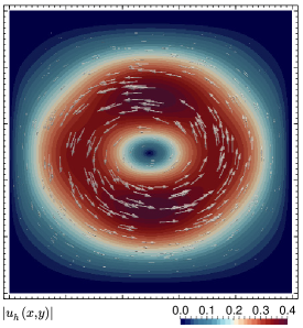
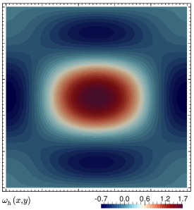
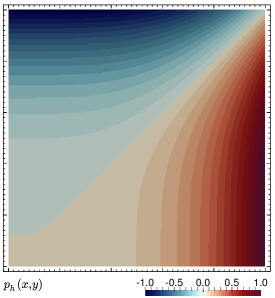
Figure 1: Experimental convergence in 2D. Lowest-order mixed finite element approximation of velocity magnitude (a), vorticity (b), and Bernoulli pressure (c) on the unit square.

We present a set of examples to confirm numerically the convergence rates anticipated in Theorem 3.2 and Theorem 4.1 . We stress that whenever $\Gamma=\partial\Omega$, the zero-mean condition enforcing the uniqueness of the Bernoulli pressure is implemented using a real Lagrange multiplier (which amounts to add one row and one column to the corresponding matrix system). Linear solves are performed with the direct method SuperLU.

Test 1: Experimental convergence in 2D.

For our first examples we produce the error history associated with the proposed mixed finite element and mixed DG approximations. Let us consider the following closed-form solutions to the Oseen equations defined on the unit square domain $\Omega=(0,1)^{2}$:

$$\boldsymbol{u}(x,y)=\!\begin{pmatrix}\sin(\pi x)^{2}\sin(\pi y)^{2}\cos(\pi y)\\ -\frac{1}{3}\sin(2\pi x)\sin(\pi y)^{3}\end{pmatrix},\quad\boldsymbol{\omega}(x,y)=\sqrt{\nu}\mathop{\mathbf{curl}}\nolimits\boldsymbol{u},\quad p(x,y)=x^{4}-y^{4}.$$

The exact velocity has zero normal component on the whole boundary, and the exact vorticity is employed to impose a non-homogeneous vorticity trace. In this example we are assuming that $\Gamma=\partial\Omega$, and the exact Bernoulli pressure fulfils the null-average condition. We consider the model parameters $\nu=0.1$ and $\sigma=10$, and the convecting velocity $\boldsymbol{\beta}$ is taken as the exact velocity solution, which in particular satisfies the bound (2.8). On a sequence of uniformly refined meshes we compute errors between the exact and approximate solutions, measured in the norms involved in the convergence analysis of Section 3. The obtained error history is reported in Table 1, where the rightmost column displays the $\ell^{\infty}-$norm of the nodal values of the velocity divergence projected to the space $\mathrm{Q}_{h}$, all approaching machine precision. The asymptotic $O(h^{k+1})$ decay of the error observed for each field variable confirms the overall optimal convergence predicted by Theorem 3.2. Sample approximate solutions generated with the lowest order method on a coarse mesh are portrayed in Figure 1.

An analogous test is now carried out to confirm numerically the convergence rates of the DG methods defined by (4.9). The same model parameters and closed-form solutions are used, and the stabilisation constants in (4.6)-(4.8) take the values $a_{11}=c_{11}=\sigma$ and $d_{11}=\nu$. The results collected in Table 2 indicate that the DG scheme converges optimally when we measure errors in the energy $\mathcal{A}-$seminorm (4.14) and in the $\mathrm{L}^{2}-$norm of the pressure. Here however, we do not expect divergence-free approximate velocities.

DoF	$\|\boldsymbol{u}-\boldsymbol{u}_{h}\|_{\mathrm{H}}$	rate	$\|\boldsymbol{\omega}-\boldsymbol{\omega}_{h}\|_{\mathrm{Z}}$	rate	$\|p-p_{h}\|_{0,\Omega}$	rate	$\|\mathop{\mathrm{div}}\nolimits\boldsymbol{u}_{h}\|_{\ell^{\infty}}$
$k=0$
34	0.1357	–	1.2943	–	0.2002	–	1.0e-14
114	0.1129	0.2654	1.0072	0.3612	0.1219	0.7161	1.3e-14
418	0.0619	0.8655	0.5623	0.8405	0.0572	1.0910	1.3e-15
1602	0.0315	0.9763	0.2869	0.9707	0.0280	1.0311	1.2e-15
6274	0.0158	0.9952	0.1441	0.9937	0.0139	1.0072	1.0e-14
24834	0.0079	0.9989	0.0721	0.9985	0.0069	1.0022	1.3e-15
98818	0.0039	0.9997	0.0361	0.9996	0.0035	1.0000	1.7e-13
$k=1$
98	0.0980	–	0.8753	–	0.0624	–	2.4e-15
354	0.0337	1.5384	0.3448	1.3441	0.0173	1.8502	4.3e-14
1346	0.0094	1.8472	0.0979	1.8173	0.0038	2.1804	3.8e-13
5250	0.0024	1.9514	0.0255	1.9403	8.3e-04	2.1952	8.0e-14
20738	6.4e-04	1.9873	0.0064	1.9835	1.9e-04	2.0791	1.2e-15
82434	2.2e-04	1.9973	0.0016	1.9960	4.8e-05	2.0233	6.2e-15
328706	3.8e-05	1.9992	4.1e-04	1.9992	1.2e-05	2.0064	1.4e-14
$k=2$
194	0.0563	–	0.5138	–	0.0237	–	1.7e-13
722	0.0078	2.8844	0.0893	2.7524	0.0024	3.2137	5.8e-14
2786	0.0011	2.9302	0.0121	2.9886	1.8e-04	3.1729	4.6e-14
10946	1.3e-04	2.9872	0.0015	2.9873	1.4e-05	3.2661	4.3e-15
43394	1.6e-05	2.9992	1.9e-04	3.0002	1.4e-06	3.2349	2.7e-15
172802	2.1e-06	2.9981	2.3e-05	3.0014	1.6e-07	3.1252	4.9e-15
689666	5.3e-07	2.9840	8.2e-06	3.0070	3.7e-08	2.9206	5.0e-14

Table 1: Test 1A: Error history (errors on a sequence of successively refined grids, convergence rates, and divergence norms) associated with the mixed finite element method (3.4) using different polynomial degrees.

DoF	$h$	$|(\boldsymbol{u}-\boldsymbol{u}_{h},\boldsymbol{\omega}-\boldsymbol{\omega}_{h},p-p_{h})|_{\mathcal{A}}$	rate	$\|p-p_{h}\|_{0,\Omega}$	rate
$k=0$
65	0.7071	0.8031	–	0.4623	–
257	0.3536	0.4321	0.8893	0.2298	0.8384
1025	0.1768	0.2343	0.8827	0.1276	0.8438
4097	0.0884	0.1217	0.9448	0.0652	0.9668
16385	0.0442	0.0616	0.9822	0.0326	1.0010
65537	0.0221	0.0302	1.0231	0.0163	1.0005
$k=1$
145	0.7071	0.4787	–	0.1847	–
577	0.3536	0.1496	1.6760	0.0529	1.8033
2305	0.1768	0.0366	2.0297	0.0133	1.9914
9217	0.0884	0.0089	2.0413	0.0033	2.0220
36865	0.0442	0.0021	2.0320	0.0008	2.0361
134696	0.0221	0.0005	2.0034	0.0002	2.0049
$k=2$
257	0.7071	0.1882	–	0.0534	–
1025	0.3536	0.0319	2.5864	0.0111	2.2722
4097	0.1768	0.0042	2.9180	0.0013	3.0093
16385	0.0884	0.0005	3.0362	0.0002	3.1105
65537	0.0442	6.16e-5	3.0640	1.81e-5	3.1510
268049	0.0221	1.03e-5	2.9973	2.78e-6	3.0076

Table 2: Test 1B: Error history associated to the DG method defined in (4.9) using increasing polynomial degree.

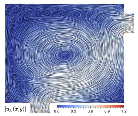
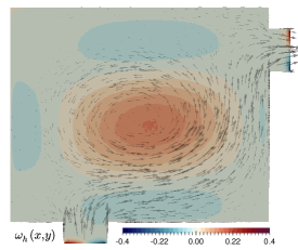
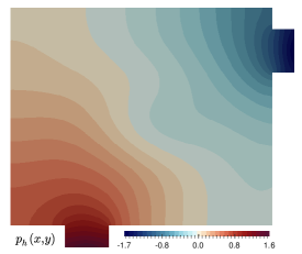
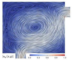
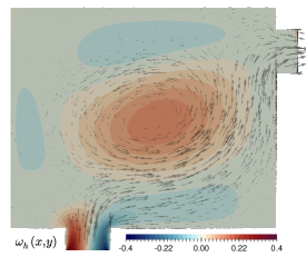
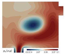
Figure 2: Second-order DG approximation of the transient flow patterns in an open cavity after one timestep (a,b,c) and after four time steps (d,e,f), using $\Delta t=0.1$ and $\nu=0.001$.

Test 2: Transient flow in an open cavity.

In this example we illustrate a more complex problem involving the non-stationary behaviour of the flow in an open 2D cavity. The main compartment of the domain consists on a rectangle $(0,1.2)\times(0,1)$ whereas smaller rectangles $(0.25,0.45)\times(-0.1,0)$ and $(1.2,1.3)\times(0.7,0.9)$ play the role of inlet and outlet channels. The domain is discretised into an unstructured mesh of 35433 triangular elements. Normal velocities and a compatible trace vorticity are imposed on the whole boundary $\Gamma=\partial\Omega$ according to

$$\boldsymbol{u}\cdot\boldsymbol{n}=\begin{cases}-75(x-0.25)(0.45-x)&\text{on $y=-0.1$},\\ 75(y-0.7)(0.9-y)&\text{on $x=1.3$},\\ 0&\text{otherwise},\end{cases}\quad\boldsymbol{\omega}\times\boldsymbol{n}=\begin{cases}75\sqrt{\nu}(0.7-2x)&\text{on $y=-0.1$},\\ -75\sqrt{\nu}(1.6-2y)&\text{on $x=1.3$},\\ 0&\text{otherwise},\end{cases}$$

that is, parabolic inlet and outlet profiles together with slip velocities elsewhere on $\partial\Omega$. We set a fluid viscosity of $\nu=0.001$ and use as initial velocity the solution adapted from the previous test $\boldsymbol{u}_{0}(x,y)=[\sin(\pi/1.3x)^{2}\sin(\pi/1.1(y+0.1))^{2}\cos(\pi/1.1(y+0.1)),-\frac{1}{3}\sin(2/1.3\pi x)\sin(\pi/1.1(y+0.1))^{3}]^{T}$. The parameter $\sigma=10$ indicates a timestep of $\Delta t=0.1$, and a backward Euler discretisation implies that we take $\boldsymbol{f}=\sigma\hat{\boldsymbol{u}}$, where $\hat{\boldsymbol{u}}$ denotes the velocity approximation at the previous iteration. The convective velocity $\boldsymbol{\beta}=\hat{\boldsymbol{u}}$ therefore needs to be updated at each iteration. At least for the initial solution we have that the convecting velocity satisfies the assumption (2.8). The simulation is run until $T_{\text{final}}=4\Delta t$ and we present in Figure 2 two snapshots of the numerical solutions at $t=\Delta t$ and $t=T_{\text{final}}$, computed with a second-order DG scheme, and using the stabilisation parameters $a_{11}=c_{11}=\sigma$ and $d_{11}=\nu$. From the velocity plots (including a line integral convolution visualisation), we can evidence the formation of a main vortex on the centre of the domain plus smaller recirculation areas that emerge on the top left and bottom left corners, together with a preferential path joining the inlet and outlet boundaries.

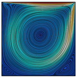
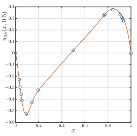
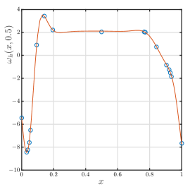
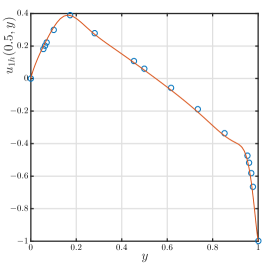
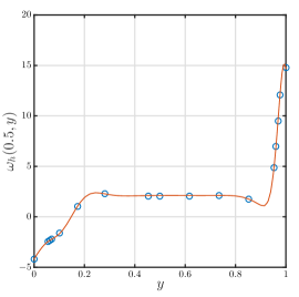
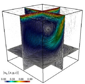
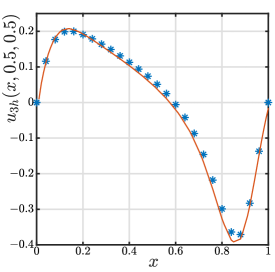
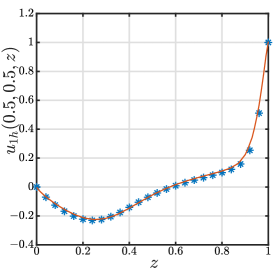
Figure 3: Test 3. Line integral convolution visualisation of velocity for the 2D cavity flow benchmark with $\nu=0.001$ (a), cuts of the vertical velocity and vorticity on the line $y=0.5$ (b,c); and horizontal velocity and vorticity on the line $x=0.5$ (d,e). The circle markers indicate benchmark values from [11]. Lowest-order approximation of velocity (f) for the 3D case with $\nu=0.0025$, shown at $t=20$; and profile of the horizontal velocity on the line $y=0.5,z=0.5$ (g), and of the vertical velocity on the line $x=0.5,y=0.5$ (h). The asterisks indicate benchmark values from [21] and all numerical approximations for this test were obtained with the lowest-order mixed finite element method.

Test 3: Lid driven cavity flow.

For this classical benchmark problem we consider zero external forces and concentrate on the case where flow recirculation occurs by Dirichlet conditions only. First we consider the two-dimensional case, where on the top lid of the unit square (at $y=1$) we set a unidirectional velocity of unit magnitude, whereas no-slip conditions and zero tangential vorticity are imposed on the remaining sides of the boundary. We set the parameters $\nu=0.001,\sigma=50$ and employ a structured mesh of 4096 elements. The initial velocity is computed from a Stokes solution (setting both $\sigma$ and $\boldsymbol{\beta}$ to zero). We compare the results obtained with our lowest-order FE scheme against the benchmark data from [11] (produced with a spectral method applied to a vorticity-based formulation). Figure 3 shows the generated velocity profile at $t=20$, having all the flow features expected for this regime. The solid lines in Figures 3-3 portray cuts of the solution on the mid-lines of the domain, whereas the circle markers indicate benchmark data. The approximate vorticity has been rescaled with $\nu^{-1/2}$ to reflect the overall agreement with the results reported in [11].

We also test the 3D implementation and formulation by conducting the same benchmark on the unit cube $\Omega=(0,1)^{3}$. Again, boundary $\Sigma$ is the top plate (defined by $z=1$), where we set tangential velocity of magnitude one, and on $\Gamma=\partial\Omega\setminus\Sigma$ we consider no-slip velocity and zero tangential vorticity. The fluid viscosity is now $\nu=0.0025$ and a structured mesh of 58752 tetrahedral elements is employed. Once again we focus on a non-stationary regime with a backward Euler scheme, now using $\sigma=10$, and proceed to update the convective velocity and the right-hand side using the velocity approximation at the previous time iteration. The velocity field for a converged solution after 200 time steps is shown in Figure 3. We can observe the expected asymmetric vortex forming parallel to the $xz$ plane (also the generation of high pressure near the corners where the Dirichlet velocity datum has a discontinuity). We have also compared our results with the benchmark values obtained in [21] (using multiquadric differential quadratures) for a Reynolds number of 400: the solid lines in Figures 3-3 show velocity profiles captured on the plane $y=0.5$, concentrating on the vertical and horizontal centrelines, where we also include the data from [21] (in asterisks) showing a reasonable match (we have rotated the data, as in their tests the unit velocity is imposed on the face $y=1$).

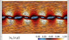
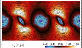
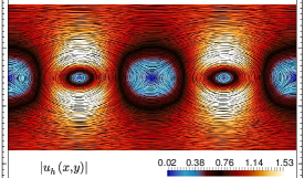
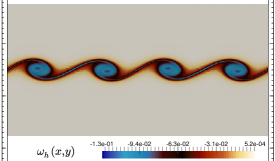
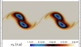
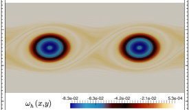
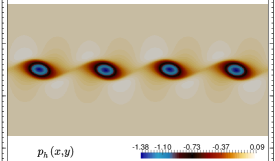
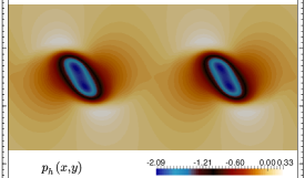
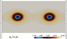
Figure 4: Test 4. Transients of the Kelvin-Helmholtz instability problem computed with the first-order DG scheme (4.9). Velocity magnitude (a-c), scalar vorticity (d-f), and Bernoulli pressure (g-i).

Test 4: Kelvin-Helmholtz mixing layer.

We close this section with a benchmark test related to the well-known vortex formation mechanisms known as the Kelvin-Helmholtz instability problem. The setup of the test follows the specifications in [31] (see also [12]), the transient Oseen equations are solved on the unit square $\Omega=(0,1)^{2}$ and the bottom and top walls constitute $\Gamma$, where we impose a free-slip velocity condition and zero vorticity. The left and right walls are regarded as a periodic boundary. The initial velocity is

$$\boldsymbol{u}=\begin{pmatrix}u_{\infty}\tanh((2y-1)/\delta_{0})-c_{n}u_{\infty}[\cos(w^{a}_{\infty}x)+\cos(w_{\infty}^{b}x)]\frac{(2y-1)}{\delta_{0}^{2}}\exp(-\frac{(y-1/2)^{2}}{\delta_{0}^{2}})\\ c_{n}u_{\infty}\exp(-\frac{(y-1/2)^{2}}{\delta_{0}^{2}})[w_{\infty}^{a}\sin(w_{\infty}^{a}x)+w_{\infty}^{b}\sin(w_{\infty}^{b}x)]\end{pmatrix},$$

with perturbation scaling $c_{n}=0.001$, reference velocity $u_{\infty}=1$, $w_{\infty}^{a}=8\pi$, $w_{\infty}^{b}=20\pi$, $\delta_{0}=1/28$. The characteristic time is $\bar{t}=\delta_{0}/u_{\infty}$, the Reynolds number is Re$=10000$, and the kinematic viscosity is $\nu=\delta_{0}u_{\infty}/\text{Re}$. We use a structured mesh of 128 segments per side, representing 131072 triangular elements, and we solve the problem using our first-order DG scheme, setting again the stabilisation constants to $a_{11}=c_{11}=\sigma=1/\Delta t$ and $d_{11}=\nu$, where the timestep is taken as $\Delta t=\bar{t}/20$. The specification of this problem implies that the solutions will be quite sensitive to the initial perturbations present in the velocity, which will amplify and consequently vortices will appear. We proceed to compute numerical solutions until the dimensionless time $t=7$, and present in Figure 4 sample solutions at three different simulation times. For visualisation purposes we zoom into the region $0.25\leq y\leq 0.75$, where all flow patterns are concentrated. In addition, a qualitative comparison against benchmark data from [31] is presented in terms of the temporal evolution of the enstrophy $E(t)$ (here we rescale $\boldsymbol{\omega}_{h}$ with $\sqrt{\nu}$ to match again the real vorticity). We also record the evolution of the palinstrophy $P(t)$, a quantity that encodes the dissipation process. These quantities are defined, respectively, as

$$E(t):=\frac{1}{2\nu}\|\boldsymbol{\omega}_{h}(t)\|^{2}_{0,\Omega},\qquad P(t):=\frac{1}{2\nu}\|\nabla\boldsymbol{\omega}_{h}(t)\|^{2}_{0,\Omega},$$

and we remark that for the palinstrophy we use the discrete gradient associated with the DG discretisation. We show these quantities in Figure 5, where also include results from [31] that correspond to coarse and fine mesh solutions of the Navier-Stokes equations using a high order scheme based on Brezzi-Douglas-Marini elements.

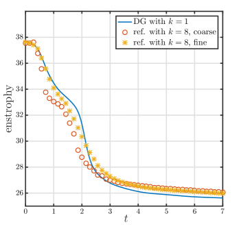
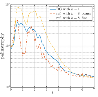
Figure 5: Test 4. Time evolution of enstrophy (a) and palinstrophy (b) in the Kelvin-Helmholtz mixing layer formation. Reference values correspond to computations from [31] using BDM elements of order 8 on a coarse and on a fine mesh.

Acknowledgements.

This work has been supported by CNRS though the PEPS programme; by CONICYT - Chile through FONDECYT project 11160706; by DIUBB, Universidad del Bío-Bío through projects 165608–3/R and 171508 GI/VC; by DIDULS, Universidad de La Serena through project PR17151; and by the EPSRC through the research grant EP/R00207X/1.

References

• [1] A. Alonso and A. Valli, An optimal domain decomposition preconditioner for low-frequency time harmonic Maxwell equations. Math. Comp., 68 (1999) 607–631.
• [2] M. Amara, D. Capatina-Papaghiuc, and D. Trujillo, Stabilized finite element method for Navier-Stokes equations with physical boundary conditions. Math. Comp., 76(259) (2007) 1195–1217.
• [3] K. Amoura, M. Azaïez, C. Bernardi, N. Chorfi, and S. Saadi, Spectral element discretization of the vorticity, velocity and pressure formulation of the Navier-Stokes problem. Calcolo, 44(3) (2007) 165–188.
• [4] V. Anaya, G.N. Gatica, D. Mora, and R. Ruiz-Baier, An augmented velocity-vorticity-pressure formulation for the Brinkman problem. Int. J. Numer. Methods Fluids, 79(3) (2015) 109–137.
• [5] V. Anaya, D. Mora, R. Oyarzúa, and R. Ruiz-Baier, A priori and a posteriori error analysis for a mixed scheme for the Brinkman problem. Numer. Math., 133(4) (2016) 781–817.
• [6] V. Anaya, D. Mora, and R. Ruiz-Baier, An augmented mixed finite element method for the vorticity-velocity-pressure formulation of the Stokes equations. Comput. Methods Appl. Mech. Engrg., 267 (2013) 261–274.
• [7] V. Anaya, D. Mora, and R. Ruiz-Baier, Pure vorticity formulation and Galerkin discretization for the Brinkman equations. IMA J. Numer. Anal., 37(4) (2017) 2020–2041.
• [8] M. Azaïez, C. Bernardi, and N. Chorfi, Spectral discretization of the vorticity, velocity and pressure formulation of the Navier-Stokes equations. Numer. Math., 104(1) (2006) 1–26.
• [9] P.B. Bochev, Analysis of least-squares finite element methods for the Navier–Stokes equations. SIAM J. Numer. Anal., 34(5) (1997) 1817–1844.
• [10] P.B. Bochev, Negative norm least-squares methods for the velocity-vorticity-pressure Navier-Stokes equations. Numer. Methods PDEs, 15(2) (1999) 237–256.
• [11] O. Botella and R. Peyret, Benchmark spectral results on the lid-driven cavity flow. Comput. & Fluids, 27(4) (1998) 421–433.
• [12] E. Burman, A. Ern, and M.A. Fernández, Fractional-step methods and finite elements with symmetric stabilization for the transient Oseen problem. ESAIM Math. Model. Numer. Anal., 51(2) (2017) 487–507.
• [13] Z. Cai and B. Chen, Least-squares method for the Oseen equation. Numer. Methods PDEs, 32 (2016) 1289–1303.
• [14] S. Caucao, D. Mora, and R. Oyarzúa, A priori and a posteriori error analysis of a pseudostress-based mixed formulation of the Stokes problem with varying density. IMA J. Numer. Anal., 36(2) (2016) 947–983.
• [15] C.L. Chang and S.-Y. Yang, Analysis of the $[L^{2},L^{2},L^{2}]$ least-squares finite element method for incompressible Oseen-type problems. Int. J. Numer. Anal. Model., 4(3-4) (2007) 402–424.
• [16] A. Çeşmelioğlu, B. Cockburn, N.C. Nguyen, and J. Peraire, Analysis of HDG methods for Oseen equations. J. Sci. Comput., 55(2) (2013) 392–431.
• [17] P. Ciarlet, The Finite Element Method for Elliptic Problems. North-Holland, Amsterdam, The Netherlands, 1978.
• [18] B. Cockburn, G. Kanschat, and D. Schötzau, The local discontinuous Galerkin method for linear incompressible fluid flow: A review. Comput. & Fluids, 34(4–5) (2005) 491–506.
• [19] B. Cockburn, G. Kanschat, and D. Schötzau, The local discontinuous Galerkin method for the Oseen equations. Math. Comp., 73(246) (2003) 569–593.
• [20] B. Cockburn, G. Kanschat, D. Schötzau, and C. Schwab, Local discontinuous Galerkin methods for the Stokes system. SIAM J. Numer. Anal., 40(1) (2002) 319–343.
• [21] H. Ding, C. Shu, K.S. Yeo, and D. Xu, Numerical computation of three-dimensional incompressible viscous flows in the primitive variable form by local multiquadric differential quadrature method. Comput. Methods Appl. Mech. Engrg., 195 (2006) 516–533.
• [22] H.-Y. Duan and G.-P. Liang, On the velocity-pressure-vorticity least-squares mixed finite element method for the 3D Stokes equations. SIAM J. Numer. Anal., 41(6) (2003) 2114–2130.
• [23] F. Dubois, M. Salaün, and S. Salmon, First vorticity-velocity-pressure numerical scheme for the Stokes problem. Comput. Methods Appl. Mech. Engrg., 192(44–46) (2003) 4877–4907.
• [24] G.N. Gatica, A Simple Introduction to the Mixed Finite Element Method. Theory and Applications. Springer Briefs in Mathematics, Springer, Cham Heidelberg New York Dordrecht London, (2014).
• [25] G.N. Gatica, L.F. Gatica, and A. Márquez, Augmented mixed finite element methods for a vorticity-based velocity–pressure–stress formulation of the Stokes problem in 2D. Int. J. Numer. Methods Fluids, 67(4) (2011) 450–477.
• [26] V. Girault and P.A. Raviart, Finite Element Methods for Navier-Stokes Equations. Theory and Algorithms. Springer-Verlag, Berlin, 1986.
• [27] S. Mohapatra and S. Ganesan, A non-conforming least squares spectral element formulation for Oseen equations with applications to Navier-Stokes equations. Numer. Funct. Anal. Optim., 37(10) (2016) 1295–1311.
• [28] R.A. Nicolaides, Existence, uniqueness and approximation for generalized saddle point problems. SIAM J. Numer. Anal., 19 (1982) 349–357.
• [29] C.W. Oseen, Über die Stokes’sche formel, und über eine verwandte Aufgabe in der Hydrodynamik, Arkiv Mat. Astr. Fys., vi(29) (1910).
• [30] M. Salaün and S. Salmon, Low-order finite element method for the well-posed bidimensional Stokes problem. IMA J. Numer. Anal., 35(1) (2015) 427–453.
• [31] P.W. Schroeder, V. John, P.L. Lederer, C. Lehrenfeld, G. Lube, and J. Schöberl, On reference solutions and the sensitivity of the 2d Kelvin–Helmholtz instability problem, arXiv: 1803.06893 (2018).
• [32] C.-C. Tsai and S.-Y. Yang, On the velocity-vorticity-pressure least-squares finite element method for the stationary incompressible Oseen problem. J. Comput. Appl. Math., 182(1) (2005) 211–232.