Beyond the Click-Through Rate: Web Link Selection with Multi-level Feedback

Abstract

The web link selection problem is to select a small subset of web links from a large web link pool, and to place the selected links on a web page that can only accommodate a limited number of links, e.g., advertisements, recommendations, or news feeds. Despite the long concerned click-through rate which reflects the attractiveness of the link itself, the revenue can only be obtained from user actions after clicks, e.g., purchasing after being directed to the product pages by recommendation links. Thus, the web links have an intrinsic multi-level feedback structure. With this observation, we consider the context-free web link selection problem, where the objective is to maximize revenue while ensuring that the attractiveness is no less than a preset threshold. The key challenge of the problem is that each link’s multi-level feedbacks are stochastic, and unobservable unless the link is selected. We model this problem with a constrained stochastic multi-armed bandit formulation, and design an efficient link selection algorithm, called Constrained Upper Confidence Bound algorithm (Con-UCB), and prove $O(\sqrt{T\ln T})$ bounds on both the regret and the violation of the attractiveness constraint. We conduct extensive experiments on three real-world datasets, and show that Con-UCB outperforms state-of-the-art context-free bandit algorithms concerning the multi-level feedback structure.

1 Introduction

With the rapid development of the Internet, web links are playing important roles in websites and mobile apps for attracting users and generating revenues. For example, e-commerce websites such as Amazon and Taobao show featured recommendation links on shopping pages to induce more purchase. Online social networks such as Facebook and Google+ constantly push links of trending topics and friends’ updates to users, so as to increase user engagement. Online media such as HBO and iQIYI present links to popular TV shows and movies on their homepages to attract more subscribers.

Due to the limited space of interest on a web page, only a finite number of links can be shown to a user when the page is browsed. This raises the web link selection problem, i.e., how to properly select a small subset of web links from a large link pool for a web page. Specifically, the web page on which the selected links are shown is called the target page. If clicked, each link directs the user to a subsequent page. This implies that web links provide a multi-level feedback to the web operator. The first level feedback refers to the likelihood that a user clicks a link, also known as the Click-Through Rate (CTR) at the target page. By tracking user actions after clicking a link, e.g., purchase or subscription, we can determine the revenue collected on the associated subsequent page, which gives the second level feedback. Since purchase or subscription can only happen after the click, the compound feedback is the product of the first-level and the second-level feedbacks. Intuitively, the first-level feedback (CTR) indicates the attractiveness of the link at the target page, while the second-level feedback indicates the potential revenue that can be collected from the subsequent page. The compound feedback reveals the compound revenue a web link can bring.

There has been a lot of research concerning the CTR of web links, e.g., Langheinrich et al. (1999); Lohtia et al. (2003). On the other hand, what happens after clicks is also worth great attention, as it generates revenue. For instance, cost per acquisition (CPA) is regarded as the optimal way for an advertiser to buy online advertising Spooner (2014). Both the attractiveness and the profitability of a website or an app are important measures Kohavi et al. (2014), because they represent the long-term and short-term benefits, respectively. This motivates us to move beyond CTR and to pursue both attractiveness and profitability simultaneously in link selection.

In this work, we consider the problem of selecting a finite number of links from a large pool for the target page, so as to maximize the total compound revenue, while keeping the total attractiveness above a certain threshold. The constraint on attractiveness (CTR) was also adopted in the literate of online advertising Kumar (2015); Mookerjee et al. (2016). In addition, we also take into consideration the fact that contextual information, e.g., user preferences, is not always available, e.g., incognito visits Aggarwal et al. (2010), cold start Elahi et al. (2016), or cookie blocking Meng et al. (2016). Thus, we do not assume any prior contextual information. We refer to our problem as the context-free web link selection problem.

Our link selection problem is challenging. First of all, the attractiveness and profitability of a link can be conflicting goals, as shown in Cai et al. (2017). As a result, while selecting links with high CTRs satisfies the attractiveness constraint, it does not necessarily guarantee that the target page will have a high total compound revenue, and vice versa. What further complicates the problem is that the multi-level feedbacks, i.e., the CTR (first-level feedback) and the potential revenue (second-level feedback) of each link, are stochastic and unobservable unless a link is selected and shown on the target page.

We formulate our problem as a constrained stochastic multiple-play multi-armed bandit problem with multi-level rewards. Specifically, there are multiple arms in the system. Each arm represents a link in the pool. Its first-level reward, second-level reward, and compound reward correspond to the first-level feedback (the CTR), the second-level feedback (the potential revenue) and the compound feedback (the compound revenue) of that link, respectively. The objective is to select a finite number of links at each time step to minimize the cumulative regret, as well as the cumulative violation of the constraint. We design a constrained bandit algorithm, Constrained Upper Confidence Bound algorithm (Con-UCB), to simultaneously achieve sub-linear regret and violation bounds.

Our main contributions are as follows. (i) We formulate the link selection problem as a constrained bandit problem with stochastic multi-level rewards (Section 3). (ii) We propose the Con-UCB algorithm (Section 4) and prove that Con-UCB ensures small regret and violation bounds with high probability, i.e., for any given failure probability $\delta\in(0,1)$, the regret and violation at time $T$ are bounded by $O(\sqrt{T\ln\frac{T}{\delta}})$ with probability at least $1-\delta$ (Section 5). (iii) We conduct extensive experiments on three real-world datasets. Our results show that Con-UCB outperforms three state-of-the-art context-free bandit algorithms, CUCB Chen et al. (2013), Exp3.M Uchiya et al. (2010), and LExp Cai et al. (2017) for the constrained link selection problem (Section 6).

2 Related work

Link selection, or website optimization, has long been an important problem. One common approach for the problem is A/B testing Xu et al. (2015); Deng et al. (2017), which splits the traffic to two web pages with different designs, and evaluates their performances. However, the overhead of A/B testing can be high when the web link pool is large, as it needs to compare different link combinations. Moreover, A/B testing does not have any loss/regret guarantees. Another approach is to model the link selection problem as a contextual multi-armed bandit problem Li et al. (2010), and to incorporate the collaborative filtering method Bresler et al. (2016); Li et al. (2016). However, these contextual bandit formulations neglect the multi-level feedback structures and do not consider any constraint.

The multiple-play multi-armed bandit problem, where multiple arms are selected in each round, has been studied from both theoretical and empirical perspectives, and many policies have been designed Uchiya et al. (2010); Chen et al. (2013); Komiyama et al. (2015); Lagrée et al. (2016). Our constrained multiple-play bandit model differs from aforementioned models in that we consider meeting the constraint on the total first-level rewards in selecting multiple arms, which is important for web link selection.

Recently, bandit with budgets Ding et al. (2013); Wu et al. (2015); Xia et al. (2016) and bandit with knapsacks Badanidiyuru et al. (2013); Agrawal and Devanur (2014) have attracted much research attention. In these problems, pulling an arm costs certain resources, and each resource has a budget. Thus, resource cost is implicitly taken into consideration during the analysis of regret in the above two formulations since the arm selection process stops when resources are depleted. In contrast, since the constraint in our model is a requirement on the average performance, our arm selection procedure can last for an arbitrary length of time, and we need to consider both the regret and the violation of the constraint during the process. Thus, while our work builds upon the results in Badanidiyuru et al. (2013) and Agrawal and Devanur (2014), the problem is different, and we study the multiple-play case rather than the single-play case. In addition, we conduct experiments on real-world datasets, which are not included in their works. On the other hand, the thresholding bandit problem in Locatelli et al. (2016) is to find the set of arms whose means are above a given threshold through pure exploration in a fixed time horizon, which is different from our model.

Our work is closest to recent work Cai et al. (2017). They assume the second-level reward is adversarial. However, it has been observed that this might not be the case in practice Pivazyan (2004), and user behavior is likely to follow certain statistical rules when the number of users is large. So we study the stochastic case. Most importantly, our algorithm guarantees performance with high probability rather than in expectation, and the regret and violation bounds are improved significantly from $O(T^{\frac{2}{3}})$ and $O(T^{\frac{5}{6}})$ in their algorithm (LExp) to both $O(\sqrt{T\ln T})$ in our algorithm (Con-UCB).

3 Model

Consider the two-level feedback context-free web link selection problem, where one needs to select $L$ links from a pool of $K$ web links, $\{l_{1},\ldots,l_{K}\},L\leq K$, to display on the target page. Each link directs users to a subsequent page. If $l_{i}$ is shown on the target page, we obtain the following feedbacks when users browse the page:

1. the click-through rate (CTR), i.e., the probability that a user clicks $l_{i}$ to visit the corresponding subsequent page,

2. the after-click revenue, i.e., the revenue collected from each user who clicks $l_{i}$ and then purchases products (or subscribes to programs) on the corresponding subsequent page.

In practice, the click-through rate and the after-click revenue are stochastic, and we do not assume any prior knowledge about their distributions or expectations. The product of the CTR and the after-click revenue is the compound revenue, i.e., the revenue that $l_{i}$ can bring if it is shown on the target page. The objective of the link selection problem is to maximize the total compound revenue of the selected $L$ links, subject to the constraint that the total CTR of these selected links is no less than a preset threshold $h>0$, where $h$ is determined by the web operator based on service requirement. An example is that in online advertising, the constraint on CTR is usually specified in the contract between the publisher (web operator) and the advertising firm Kumar (2015); Mookerjee et al. (2016).

To address the link selection problem, we formulate it as a constrained stochastic multi-armed bandit problem with multiple plays, where each arm has a two-level reward structure. In this formulation, each time step is a short duration and each arm corresponds to a specific web link. Thus, the set of arms can be written as $\mathcal{K}=\{1,\ldots,K\}$. Each arm $i$ is associated with two sequences of random variables, $\{a_{i}^{t}\}_{t=1}^{T}$ and $\{b_{i}^{t}\}_{t=1}^{T}$, where $a_{i}^{t}$ characterizes arm $i$’s first-level reward (CTR) at time $t$, and $b_{i}^{t}$ characterizes arm $i$’s second-level reward (after-click revenue). We assume that for any $i\in\mathcal{K}$, both $\{a_{i}^{t}\}_{t=1}^{T}$ and $\{b_{i}^{t}\}_{t=1}^{T}$ are sequences of i.i.d. random variables. The expectations of $a_{i}^{t}$ and $b_{i}^{t}$ are denoted by $a_{i}=\operatorname*{\mathbb{E}}[a_{i}^{t}]$ and $b_{i}=\operatorname*{\mathbb{E}}[b_{i}^{t}]$, $i\in\mathcal{K}$. We also assume that $a_{i}^{t}$ is independent of $b_{i}^{t}$ for $i\in\mathcal{K}$, $t\geq 1$. Thus, the compound reward of arm $i$ at time $t$ is $g_{i}^{t}=a_{i}^{t}b_{i}^{t}$ with mean $g_{i}=\operatorname*{\mathbb{E}}[g_{i}^{t}]=a_{i}b_{i}$. Denote $\bm{a}=(a_{1},\ldots,a_{K})$ and $\bm{g}=(g_{1},\ldots,g_{K})$. Without loss of generality, we assume that $a_{i}^{t}\in[0,1]$ and $b_{i}^{t}\in[0,1]$.

As mentioned above, the distributions or expectations of the two-level reward for any arm are unknown beforehand. At each time step $t$, an algorithm $\pi$ selects a set of $L\leq K$ arms $\mathcal{I}_{t}(\pi)\subset\mathcal{K}$, and observes the first level reward $a_{i}^{t}$ as well as the second level reward $b_{i}^{t}$ for each arm $i\in\mathcal{I}_{t}(\pi)$. The optimal policy is the one that maximizes the expected total compound reward of the selected $L$ arms, while keeping the total first level reward above the preset threshold $0<h<L$.

The optimal policy is not limited to deterministic policies as in traditional multi-armed bandit problems Auer et al. (2002); Bubeck et al. (2012), but can be randomized, i.e., a distribution on the possible selections $\mathcal{I}_{t}$. In practice, the number of web links $K$ can be very large, and the number of possible selections of links at each time step can be as large as $\binom{K}{L}$, which makes it complicated to consider randomized policies. To simplify the problem, we represent a randomized policy with a probabilistic selection vector $\bm{x}=(x_{1},\ldots,x_{i},\ldots,x_{K}),\bm{1}^{\intercal}\bm{x}=L$, where $x_{i}\in[0,1]$ is the probability of selecting arm $i$ and $\bm{1}=(1,\ldots,1)$ is the one vector. At each time $t$, the selection set $\mathcal{I}_{t}(\bm{x})$ under a randomized policy $\bm{x}$ is generated via a dependent rounding procedure Gandhi et al. (2006), which guarantees the probability that $i\in\mathcal{I}_{t}(\bm{x})$ is $x_{i}$ (see Section 4).

The set of randomized policies can be denoted by $\mathcal{X}=\{\bm{x}\in\mathbb{R}^{K}|0\leq x_{i}\leq 1,\bm{1}^{\intercal}\bm{x}=L\}$. Thus, the optimal stationary randomized policy is

$$\bm{x}^{*}=\operatorname*{arg\,\max}_{\bm{x}^{\intercal}\bm{a}\geq h}\bm{x}^{\intercal}\bm{g}.$$ (1)

Our objective is to design an algorithm $\pi$ to decide the selection set $\mathcal{I}_{t}(\pi)$ for $t=1,\ldots,T$, such that the regret, i.e., the accumulated difference $\textmd{Reg}_{\pi}(T)$ between the compound reward under $\pi$ and that under the optimal policy, is minimized. Specifically,

$$\textmd{Reg}_{\pi}(T)=T{\bm{x}^{*}}^{\intercal}\bm{g}-\sum_{t=1}^{T}\sum_{i\in\mathcal{I}_{t}(\pi)}g_{i}^{t}.$$ (2)

Note that the total first-level reward of arms in $\mathcal{I}_{t}(\pi)$ may violate the constraint, especially when $t$ is small and we have little information about the arms. To measure the overall violation of the constraint at time $T$, we define violation of algorithm $\pi$ as,

$$\textmd{Vio}_{\pi}(T)=[hT-\sum_{t=1}^{T}\sum_{i\in\mathcal{I}_{t}(\pi)}a_{i}^{t}]_{+},$$ (3)

where $[x]_{+}=\max(x,0)$. Note that when designing link selection algorithms, we should take both the regret and violation into consideration, so as to achieve both sub-linear regret and sub-linear violation with respect to $T$. Also, note that our model can be generalized to link selection problems with $n$-level ($n>2$) feedback structures, by taking a subsequent page as a new target page and select links for it with the above model, and so on.

4 Algorithm

In this section, we present our Constrained Upper Confidence Bound algorithm (Con-UCB), and describe its details in Algorithm 1. Let $H_{t}=\{\mathcal{I}_{\tau},a_{i}^{\tau},b_{i}^{\tau}:i\in\mathcal{I}_{\tau},1\leq\tau\leq t\}$ denote the historical information of chosen actions and observations up to time $t$. Define the empirical average first-level reward and compound reward for each arm $i$ as

$$\bar{a}_{i}^{t}=\frac{\sum_{\tau<t,i\in\mathcal{I}_{\tau}}a_{i}^{\tau}}{N_{i}^{t}+1},$$ (4)

$$\bar{g}_{i}^{t}=\frac{\sum_{\tau<t,i\in\mathcal{I}_{\tau}}g_{i}^{\tau}}{N_{i}^{t}+1},$$

where $N_{i}^{t}$ is the number that arm $i$ is played before time $t$. Define $R(\mu,n)=\sqrt{\frac{\gamma\mu}{n}}+\frac{\gamma}{n}$ as in Kleinberg et al. (2008) where $\gamma$ is a constant. In Con-UCB, we use the following Upper Confidence Bounds for the unknown rewards Agrawal and Devanur (2014):

$$\hat{a}_{i}^{t}= \min\{1,\bar{a}_{i}^{t}+2R(\bar{a}_{i}^{t},N_{i}^{t}+1)\},$$

$$\hat{g}_{i}^{t}= \min\{1,\bar{g}_{i}^{t}+2R(\bar{g}_{i}^{t},N_{i}^{t}+1)\}.$$

Denote $\bar{\bm{a}}^{t}=(\bar{a}_{1}^{t},\ldots,\bar{a}_{K}^{t})$, $\bar{\bm{g}}^{t}=(\bar{g}_{1}^{t},\ldots,\bar{g}_{K}^{t})$, and $\hat{\bm{a}}^{t}=(\hat{a}_{1}^{t},\ldots,\hat{a}_{K}^{t})$, $\hat{\bm{g}}^{t}=(\hat{g}_{1}^{t},\ldots,\hat{g}_{K}^{t})$. In the initialization step of Algorithm 1, $\gamma$ is set to $72\ln\frac{8KT}{\delta}$, where $\delta\in(0,1)$ is an input parameter, i.e., the allowed failure probability.

Specifically, in each round, Con-UCB solves the optimization problem (5) to get the probabilistic selection vector $\bm{x}_{t}$ (line 5). Notice that (5) is similar to the original constrained optimization problem (1) but uses the Upper Confidence Bounds to replace the unknown rewards. Then, $\mathcal{I}_{t}$ is generated via a dependent rounding procedure. In line 7 we receive the two-level rewards $a_{i}^{t}$ and $b_{i}^{t}$ for arms in $\mathcal{I}_{t}$ and update the empirical average rewards to get the Upper Confidence Bounds for the next round.

Algorithm 1 Constrained Upper Confidence Bound

1:$K$, $L$, $h$, $\delta\in(0,1)$.

2:Selected arm set for each round.

3:Set $\gamma=72\ln\frac{8KT}{\delta},\bar{\bm{g}}^{1}=\bm{0},\bar{\bm{a}}^{1}=\bm{0}$, and $N_{i}^{1}=0,\forall i$.

4:for $t=1,2,\dots,T$ do

5:      Solve the following linear optimization problem:

$$\bm{x}_{t}={\arg\max}_{\bm{x}^{\intercal}\hat{\bm{a}}^{t}\geq h,\bm{x}\in\mathcal{X}}\bm{x}^{\intercal}\hat{\bm{g}}^{t}.$$ (5)

     If (5) has no feasible solution, set $\bm{x}_{t}\in\mathcal{X}$ arbitrarily.

6:     Set $\mathcal{I}_{t}=\text{{DependentRounding}}(L,\bm{x}_{t}).$

7:      Receive $a_{i}^{t}$ and $b_{i}^{t}$ for $i\in\mathcal{I}_{t}$. Update

$$N_{i}^{t+1} =\begin{cases}N_{i}^{t}+1,\text{ $i\in\mathcal{I}_{t}$},\\ N_{i}^{t},\text{\qquad$i\notin\mathcal{I}_{t}$},\end{cases}$$

$$\bar{g}_{i}^{t+1} =\begin{cases}[\bar{g}_{i}^{t}(N_{i}^{t}+1)+g_{i}^{t}]/(N_{i}^{t+1}+1),&\text{$i\in\mathcal{I}_{t}$},\\ \bar{g}_{i}^{t},&\text{$i\notin\mathcal{I}_{t}$},\end{cases}$$

$$\bar{a}_{i}^{t+1} =\begin{cases}[\bar{a}_{i}^{t}(N_{i}^{t}+1)+a_{i}^{t}]/(N_{i}^{t+1}+1),&\text{$i\in\mathcal{I}_{t}$},\\ \bar{a}_{i}^{t},&\text{$i\notin\mathcal{I}_{t}$}.\end{cases}$$

8:end for

9:function DependentRounding($L,\bm{x}$)

10:     while exists $i$ such that $0<x_{i}<1$ do

11:         Find $i,j,i\neq j$, such that $x_{i},x_{j}\in(0,1)$.

12:         Set $p=\min\{1-x_{i},x_{j}\}$, $q=\min\{x_{i},1-x_{j}\}$.

13:         Update $x_{i}$ and $x_{j}$ as

14:         $(x_{i},x_{j})=\begin{cases}(x_{i}+p,x_{j}-p),\text{ probability }\frac{q}{p+q};\\ (x_{i}-q,x_{j}+q),\text{ probability }\frac{p}{p+q}.\end{cases}$

15:     end while

16:     return $\mathcal{I}=\{i\,|\,x_{i}=1,1\leq i\leq K\}$.

17:end function

5 Theoretical Analysis

In this section, we bound the regret and violation of Algorithm 1. We will make use of the concentration inequalities in the following lemmas.

Lemma 1 (Azuma-Hoeffding inequality Azuma (1967)).

Suppose $\{Y_{n}:n=0,1,2,3,\dots\}$ is a martingale and $|Y_{n}-Y_{n-1}|\leq c_{n}$ almost surely, then with probability at least $1-2e^{-\frac{d^{2}}{2\sum_{j=1}^{n}c_{j}^{2}}}$, we have

$$|Y_{n}-Y_{0}|\leq d.$$

Lemma 2 (Kleinberg et al. (2008); Badanidiyuru et al. (2013); Agrawal and Devanur (2014)).

Consider $n$ i.i.d random variables $Z_{1},\dots,Z_{n}$ in $[0,1]$ with expectation $z$. Let $\mu$ denote their empirical average. Then, for any $\gamma>0$, with probability at least $1-2e^{-\frac{1}{72}\gamma}$, we have

$$|\mu-z|\leq R(\mu,n),$$

where $R(\mu,n)=\sqrt{\frac{\gamma\mu}{n}}+\frac{\gamma}{n}$.

The following lemma is a corollary of Lemma 2.

Lemma 3.

Define the empirical averages $\bar{a}_{i}^{t}$ and $\bar{g}_{i}^{t}$ as in (4). Then, for every $i$ and $t$, with probability at least $1-2e^{-\frac{1}{72}\gamma}$, we have

$$|\bar{a}_{i}^{t}-a_{i}|\leq 2R(\bar{a}_{i}^{t},N_{i}^{t}+1),$$

where $\gamma\geq 1$. The same result holds between $\bar{g}_{i}^{t}$ and $g_{i}$.

Proof.

For every $i$ and $t$, applying Lemma 2, we have that, with probability at least $1-2e^{-\frac{1}{72}\gamma}$,

$$|\frac{N_{i}^{t}+1}{N_{i}^{t}}\bar{a}_{i}^{t}-a_{i}| \leq R(\frac{N_{i}^{t}+1}{N_{i}^{t}}\bar{a}_{i}^{t},N_{i}^{t}),$$

$$|\bar{a}_{i}^{t}-a_{i}+\frac{a_{i}}{N_{i}^{t}+1}| \leq\frac{N_{i}^{t}}{N_{i}^{t}+1}R(\frac{N_{i}^{t}+1}{N_{i}^{t}}\bar{a}_{i}^{t},N_{i}^{t}).$$

This implies that

$$|\bar{a}_{i}^{t}-a_{i}| \leq\frac{N_{i}^{t}}{N_{i}^{t}+1}(\sqrt{\frac{\gamma(N_{i}^{t}+1)\bar{a}_{i}^{t}}{N_{i}^{t}\cdot N_{i}^{t}}}+\frac{\gamma}{N_{i}^{t}})+\frac{a_{i}}{N_{i}^{t}+1},$$

$$=R(\bar{a}_{i}^{t},N_{i}^{t}+1)+\frac{a_{i}}{N_{i}^{t}+1},$$

$$\leq 2R(\bar{a}_{i}^{t},N_{i}^{t}+1).$$

The last inequality holds because $a_{i}\leq 1\leq\gamma$. ∎

Based on the above lemmas, we obtain the following properties about Con-UCB.

Lemma 4.

By running Con-UCB for $T$ rounds with $\gamma=72\ln\frac{8KT}{\delta}$, with probability at least $1-\delta$, the following results hold simultaneously:

$$a_{i}\leq\hat{a}_{i}^{t},\forall 1\leq i\leq K,\forall 1\leq t\leq T,$$ (6)

$$|\sum_{t=1}^{T}(\sum_{i\in\mathcal{I}_{t}}a_{i}^{t}-\bm{x}_{t}^{\intercal}\hat{\bm{a}}^{t})|=O(L\sqrt{KT\ln\frac{KT}{\delta}}),$$ (7)

$$g_{i}\leq\hat{g}_{i}^{t},\forall 1\leq i\leq K,\forall 1\leq t\leq T,$$ (8)

$$|\sum_{t=1}^{T}(\sum_{i\in\mathcal{I}_{t}}g_{i}^{t}-\bm{x}_{t}^{\intercal}\hat{\bm{g}}^{t})|=O(L\sqrt{KT\ln\frac{KT}{\delta}}).$$ (9)

Proof.

See Appendix A. ∎

From Lemma 4, we can obtain the regret and violation bounds for Con-UCB.

Theorem 1.

For all $T>0$, let $\gamma=72\ln\frac{8KT}{\delta}$. By running Con-UCB, we have with probability at least $1-\delta$ that,

$$\textmd{Reg}(T)= O(L\sqrt{KT\ln\frac{KT}{\delta}}),$$

$$\textmd{Vio}(T)= O(L\sqrt{KT\ln\frac{KT}{\delta}}).$$

Proof.

We bound the regret and violation using (6) to (9), which were shown to hold with probability at least $1-\delta$ in Lemma 4.

From (6) we know for all $t$, $\bm{x}^{*}$ is a feasible solution of the optimization problem (5), i.e., ${\bm{x}^{*}}^{\intercal}\hat{\bm{a}}^{t}\geq{\bm{x}^{*}}^{\intercal}\bm{a}\geq h$. Then, for all $1\leq t\leq T$, we have,

$$\bm{x}_{t}^{\intercal}\hat{\bm{g}}^{t}\geq{\bm{x}^{*}}^{\intercal}\hat{\bm{g}}^{t}\geq{\bm{x}^{*}}^{\intercal}\bm{g},$$ (10)

where the last inequality follows from (8). Combining (9) and (10), we have

$$\textmd{Reg}(T)=O(L\sqrt{KT\ln\frac{KT}{\delta}}).$$

On the other hand, since for all $t$, (5) has a feasible solution $\bm{x}^{*}$, we know $\bm{x}_{t}^{\intercal}\hat{\bm{a}}^{t}\geq h,1\leq t\leq T$. Then with (7), we can get

$$\textmd{Vio}(T)=O(L\sqrt{KT\ln\frac{KT}{\delta}}).$$

This completes the proof. ∎

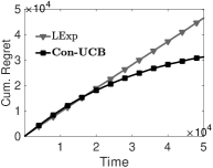
(a) Cumulative regret

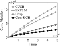
(b) Cumulative violation

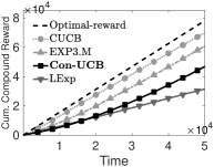
(c) Cum. compound reward

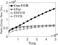
(d) Reward/Violation ratio

Figure 1: Experiment results on the Coupon-Purchase dataset. $K=271,L=15,h=4,\delta=0.01$.

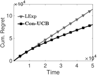
(a) Cumulative regret

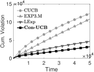
(b) Cumulative violation

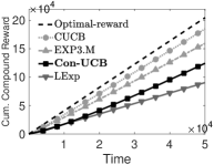
(c) Cum. compound reward

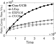
(d) Reward/Violation ratio

Figure 2: Experiment results on the Ad-Clicks dataset. $K=225,L=20,h=10,\delta=0.02$.

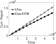
(a) Cumulative regret

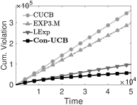
(b) Cumulative violation

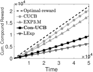
(c) Cum. compound reward

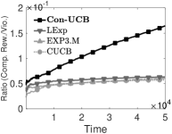
(d) Reward/Violation ratio

Figure 3: Experiment results on the edX-Course dataset. $K=290,L=60,h=10,\delta=0.05$.

6 Experiments

We conduct experiments on three real-world datasets to evaluate the performance of Con-UCB. Two datasets, Coupon-Purchase Kaggle (2016) and Ad-Clicks Kaggle (2015), with $271$ coupons and $225$ ads respectively, are shown to have a two-level feedback structure in Cai et al. (2017). In particular, for each coupon in Coupon-Purchase, a user who clicks the link to the coupon can decide whether to purchase that coupon; for each ad in Ad-Clicks, a user who clicks the link to the ad can decide whether to request the corresponding seller’s phone number. Thus, for Coupon-Purchase (Ad-Clicks), the first-level feedback is the CTR of each coupon (the CTR of each ad) and the second-level feedback is the purchase rate of each coupon (the phone request rate of each ad). The third dataset, edX-Course, is extracted from the data on $290$ Harvard and MIT edX online courses Chuang and Ho (2016). In particular, for the $290$ online courses, we obtain course participation rates by normalizing the numbers of participants using min-max scaling and treat the course participation rates as the first-level feedback; we calculate course certification rates by dividing the numbers of certified participants by the numbers of participants, and treat the course certification rates as the second-level feedback.

We treat the coupons, ads, and courses as different sets of arms. To simulate the real-time two-level feedback of the coupons, ads, and courses, we generate the first-level reward of each arm (coupon, ad, and course) using a Bernoulli variable with mean taken from the first-level feedback (coupon CTR, ad CTR, and course participation rate) in the three datasets, and generate the second-level reward of each arm using another independent Bernoulli variable with mean taken from the second-level feedback (coupon purchase rate, ad phone request rate, and course certification rate).

For comparison purposes, we implement three state-of-the-art bandit algorithms that can select multiple arms $(L\geq 1)$ at each round as baselines, i.e., CUCB Chen et al. (2013), Exp3.M Uchiya et al. (2010) and LExp Cai et al. (2017). Specifically, CUCB selects the top-$L$ arms with the $L$ highest UCB indices $\bar{g}_{i}^{t}+\sqrt{3\ln t/(2N_{i}^{t})}$. Exp3.M selects $L$ arms using exponential weights on the compound rewards of $K$ arms, and LExp selects arms using exponential weights based on the Lagrangian function of reward and violation of $K$ arms.

For the three datasets, we run the three algorithms together with Con-UCB for $50,000$ rounds with parameter settings as shown in Figure 1–3, respectively. In particular, the parameters of Exp3.M and LExp are set in accordance with Corollary 1 of Uchiya et al. (2010) and Theorem 1 of Cai et al. (2017), respectively. We compare the cumulative regrets $t{\bm{x}^{*}}^{\intercal}\bm{g}-\sum_{\tau=1}^{t}\sum_{i\in\mathcal{I}_{\tau}}g_{i}^{\tau}$ of LExp and Con-UCB at each round $t$, where the optimal policy $\bm{x}^{*}$ is computed from the means of the two-level feedback taken from each datatset. (Note that the regrets of CUCB and Exp3.M are not considered since they both have an unconstrained optimal policy, and therefore have different regret definitions from LExp and Con-UCB.) We also compare the cumulative violations $\sum_{\tau=1}^{t}(h-\sum_{i\in\mathcal{I}_{\tau}}a_{i}^{\tau})_{+}$ and the cumulative compound rewards $\sum_{\tau=1}^{t}\sum_{i\in\mathcal{I}_{\tau}}g_{i}^{\tau}$ of the four algorithms. To put things into perspective, we compare the ratios between the cumulative rewards and the cumulative violations of all the algorithms. Such ratios show how much reward an algorithm can gain for each unit violation it has made.

The experiment results are averaged over $200$ runs of each algorithm and illustrated in Figure 1–3. Figure 1(a) shows that the cumulative regret of Con-UCB is much lower than that of LExp on the Coupon-Purchase dataset. This shows that Con-UCB can reduce the regret significantly by selecting arms using UCB-based optimization instead of exponential weights as in LExp. Figure 1(b) and Figure 1(c) show the cumulative violations and the cumulative rewards of the four algorithms. In particular, the Optimal-reward in Figure 1(c) shows the cumulative reward $t{\bm{x}^{*}}^{\intercal}\bm{g}$ of the optimal policy $\bm{x}^{*}$ at each round $t$. As shown in Figure 1(c), CUCB and Exp3.M have larger cumulative rewards than Con-UCB and LExp, as both CUCB and Exp3.M neglect the threshold constraint and thereby blindly selecting arms that maximize the cumulative rewards. Therefore, both CUCB and Exp3.M incur huge cumulative violations as shown in Figure 1(b). Moreover, Con-UCB has a larger cumulative reward and a lower cumulative violation than LExp. This matches our theoretical results that Con-UCB has smaller regret as well as violation bounds than LExp. Figure 1(d) shows that Con-UCB achieves the largest reward/violation ratios among the four algorithms. This means that Con-UCB achieves the best tradeoff between rewards and violations and accumulates most reward for each unit violation it incurs.

We have similar experiment results on Ad-Clicks and edX-Course to those on Coupon-Purchase. As shown in Figure 2 and Figure 3, Con-UCB achieves lower cumulative regret and higher cumulative rewards than LExp, and has the lowest cumulative violations and largest reward/violation ratios among all algorithms. Due to space limit, we omit the details.

In summary, our experiment results are consistent with our theoretical analysis and demonstrate the effectiveness of our Con-UCB algorithm in selecting arms with high cumulative rewards as well as low cumulative violations, thus achieving a good tradeoff between the reward and the violation.

7 Conclusion

In this paper, we consider the web link selection problem with multi-level feedback. We formulate it as a constrained multiple-play stochastic multi-armed bandit problem with multi-level reward. We design an efficient algorithm Con-UCB for solving the problem, and prove that for any given allowed failure probability $\delta\in(0,1)$, with probability at least $1-\delta$, Con-UCB guarantees $O(\sqrt{T\ln\frac{T}{\delta}})$ regret and violation bounds. We conduct extensive experiments on three real-world datasets to compare our Con-UCB algorithm with state-of-the-art context-free bandit algorithms. Experiment results show that Con-UCB balances regret and violation better than the other algorithms and outperforms LExp in both regret and violation.

Appendix A Proof of Lemma 4

Proof.

We first show that (6) and (7) hold with probability at least $1-\frac{\delta}{2}$. Notice that $\gamma=72\ln\frac{8KT}{\delta}\geq 1$. From Lemma 3, by taking a union bound over all $i\in\mathcal{K}$ and all $t$, we obtain that for all $1\leq i\leq K$ and all $1\leq t\leq T$, with probability at least $1-2KTe^{-\frac{1}{72}\gamma}=1-\frac{\delta}{4}$,

$$|\bar{a}_{i}^{t}-a_{i}|\leq 2R(\bar{a}_{i}^{t},N_{i}^{t}+1),$$ (11)

which means

$$a_{i}\leq\bar{a}_{i}^{t}+2R(\bar{a}_{i}^{t},N_{i}^{t}+1).$$ (12)

Recall that $\hat{a}_{i}^{t}=\min\{1,\bar{a}_{i}^{t}+2R(\bar{a}_{i}^{t},N_{i}^{t}+1)\}$. Together with (12), we see that (6) holds.

To prove (7), we define a series of random variables $Z_{t},1\leq t\leq T$ as

$$Z_{t}=\sum_{i\in\mathcal{I}_{t}}a_{i}^{t}-\sum_{i\in\mathcal{I}_{t}}a_{i}.$$

We know $\operatorname*{\mathbb{E}}\{Z_{t}|H_{t-1}\}=0$ and $|Z_{t}|\leq L$. Recall that $H_{t}$ denotes the historical information of chosen actions and observations up to time $t$. Thus, by Lemma 1, we get, with probability at least $1-\frac{\delta}{8}$,

$$|\sum_{t=1}^{T}(\sum_{i\in\mathcal{I}_{t}}a_{i}^{t}-\sum_{i\in\mathcal{I}_{t}}a_{i})|\leq L\sqrt{2T\ln\frac{16}{\delta}}.$$ (13)

Similarly, with probability at least $1-\frac{\delta}{8}$,

$$|\sum_{t=1}^{T}(\sum_{i\in\mathcal{I}_{t}}\hat{a}_{i}^{t}-\bm{x}_{t}^{\intercal}\hat{\bm{a}}^{t})|\leq L\sqrt{2T\ln\frac{16}{\delta}}.$$ (14)

Next we bound $|\sum_{t=1}^{T}\sum_{i\in\mathcal{I}_{t}}(\hat{a}_{i}^{t}-a_{i})|$. Notice that (11) also implies that for all $i$ and $t$,

$$|\hat{a}_{i}^{t}-a_{i}|\leq 4R(\bar{a}_{i}^{t},N_{i}^{t}+1).$$

Let $\tau(i,n)$ denote the time that arm $i$ is played for the $n$th time. We have

$$|\sum_{t=1}^{T}\sum_{i\in\mathcal{I}_{t}}(\hat{a}_{i}^{t}-a_{i})|\leq\sum_{t=1}^{T}\sum_{i\in\mathcal{I}_{t}}4R(\bar{a}_{i}^{t},N_{i}^{t}+1)$$

$$=\sum_{i=1}^{K}\sum_{n=1}^{N_{i}^{T+1}}4R(\bar{a}_{i}^{\tau(i,n)},n)$$

$$\leq\sum_{i=1}^{K}\sum_{n=1}^{N_{i}^{T+1}}4(\sqrt{\frac{\gamma}{n}}+\frac{\gamma}{n})$$

$$=O(\sum_{i=1}^{K}(\sqrt{\gamma N_{i}^{T+1}}+\gamma\ln N_{i}^{T+1}))$$

$$\leq O(\sqrt{K}\sqrt{\sum_{i=1}^{K}\gamma N_{i}^{T+1}}+K\gamma\ln T)$$ (15)

$$=O(L\sqrt{KT\ln\frac{KT}{\delta}}),$$ (16)

where (15) follows from the Cauchy-Schwarz inequality and (16) follows from the fact that $\sum_{i=1}^{K}N_{i}^{T+1}=LT$. Thus, (13), (14) and (16) together give

$$|\sum_{t=1}^{T}(\sum_{i\in\mathcal{I}_{t}}a_{i}^{t}-\bm{x}_{t}^{\intercal}\hat{\bm{a}}^{t})|=O(L\sqrt{KT\ln\frac{KT}{\delta}}).$$

Repeating the same analysis, we can show that (8) and (9) also hold with probability at least $1-\frac{\delta}{2}$. Then, we can prove the lemma using the union bound. ∎

References

- Aggarwal et al. [2010] Gaurav Aggarwal, Elie Bursztein, Collin Jackson, and Dan Boneh. An analysis of private browsing modes in modern browsers. In Proceedings of the 19th USENIX conference on Security, 2010.
- Agrawal and Devanur [2014] Shipra Agrawal and Nikhil R. Devanur. Bandits with concave rewards and convex knapsacks. In Proceedings of ACM EC, 2014.
- Anantharam et al. [1987] Venkatachalam Anantharam, Pravin Varaiya, and Jean Walrand. Asymptotically efficient allocation rules for the multiarmed bandit problem with multiple plays-part i: Iid rewards. IEEE Transactions on Automatic Control, 32(11):968–976, 1987.
- Auer et al. [2002] Peter Auer, Nicolo Cesa-Bianchi, and Paul Fischer. Finite-time analysis of the multiarmed bandit problem. Machine learning, 47(2-3):235–256, 2002.
- Azuma [1967] Kazuoki Azuma. Weighted sums of certain dependent random variables. Tohoku Mathematical Journal, 19:357–367, 1967.
- Badanidiyuru et al. [2013] Ashwinkumar Badanidiyuru, Robert Kleinberg, and Aleksandrs Slivkins. Bandits with knapsacks. In Proceedings of FOCS, 2013.
- Bresler et al. [2016] Guy Bresler, Devavrat Shah, and Luis Filipe Voloch. Collaborative filtering with low regret. In Proceedings of ACM SIGMETRICS, 2016.
- Bubeck et al. [2012] Sébastien Bubeck, Nicolo Cesa-Bianchi, et al. Regret analysis of stochastic and nonstochastic multi-armed bandit problems. Foundations and Trends® in Machine Learning, 5(1):1–122, 2012.
- Cai et al. [2017] Kechao Cai, Kun Chen, Longbo Huang, and John C. S. Lui. Multi-level feedback web links selection problem: Learning and optimization. In Proceedings of ICDM, 2017.
- Chen et al. [2013] Wei Chen, Yajun Wang, and Yang Yuan. Combinatorial multi-armed bandit: General framework, results and applications. In Proceedings of ICML, 2013.
- Chuang and Ho [2016] Isaac Chuang and Andrew Dean Ho. Harvardx and mitx: Four years of open online courses–fall 2012-summer 2016. SSRN, 2016.
- Deng et al. [2017] Alex Deng, Jiannan Lu, and Jonthan Litz. Trustworthy analysis of online a/b tests: Pitfalls, challenges and solutions. In Proceedings of WSDM, 2017.
- Ding et al. [2013] Wenkui Ding, Tao Qin, Xu-Dong Zhang, and Tie-Yan Liu. Multi-armed bandit with budget constraint and variable costs. In AAAI, 2013.
- Elahi et al. [2016] Mehdi Elahi, Francesco Ricci, and Neil Rubens. A survey of active learning in collaborative filtering recommender systems. Computer Science Review, 20:29–50, 2016.
- Gandhi et al. [2006] Rajiv Gandhi, Samir Khuller, Srinivasan Parthasarathy, and Aravind Srinivasan. Dependent rounding and its applications to approximation algorithms. Journal of the ACM (JACM), 53(3):324–360, 2006.
- Kaggle [2015] Kaggle. Avito context ad clicks, 2015. https://www.kaggle.com/c/avito-context-ad-clicks.
- Kaggle [2016] Kaggle. Coupon purchase data, 2016. https://www.kaggle.com/c/coupon-purchase-prediction.
- Kleinberg et al. [2008] Robert Kleinberg, Aleksandrs Slivkins, and Eli Upfal. Multi-armed bandits in metric spaces. In Proceedings of STOC, 2008.
- Kohavi et al. [2014] Ron Kohavi, Alex Deng, Roger Longbotham, and Ya Xu. Seven rules of thumb for web site experimenters. In Proceedings of SIGKDD, 2014.
- Komiyama et al. [2015] J. Komiyama, J. Hondaand, and H. Nakagawa. Optimal regret analysis of thompson sampling in stochastic multi-armed bandit problem with multiple plays. In Proceedings of ICML, 2015.
- Kumar [2015] Subodha Kumar. Optimization Issues in Web and Mobile Advertising: Past and Future Trends. Springer, 2015.
- Lagrée et al. [2016] Paul Lagrée, Claire Vernade, and Olivier Cappe. Multiple-play bandits in the position-based model. In Proceedings of NIPS, 2016.
- Langheinrich et al. [1999] Marc Langheinrich, Atsuyoshi Nakamura, Naoki Abe, Tomonari Kamba, and Yoshiyuki Koseki. Unintrusive customization techniques for web advertising. Computer Networks, 31(11):1259–1272, 1999.
- Li et al. [2010] L. Li, W. Chu, J. Langford, and R.E. Schapire. A contextual-bandit approach to personalized news article recommendation. In Proceedings of WWW, 2010.
- Li et al. [2016] Shuai Li, Alexandros Karatzoglou, and Claudio Gentile. Collaborative filtering bandits. In Proceedings of SIGIR, 2016.
- Locatelli et al. [2016] Andrea Locatelli, Maurilio Gutzeit, and Alexandra Carpentier. An optimal algorithm for the thresholding bandit problem. In Proceedings of ICML, 2016.
- Lohtia et al. [2003] Ritu Lohtia, Naveen Donthu, and Edmund K Hershberger. The impact of content and design elements on banner advertising click-through rates. Journal of advertising Research, 43(4):410–418, 2003.
- Meng et al. [2016] Wei Meng, Byoungyoung Lee, Xinyu Xing, and Wenke Lee. Trackmeornot: Enabling flexible control on web tracking. In Proceedings of WWW, 2016.
- Mookerjee et al. [2016] Radha Mookerjee, Subodha Kumar, and Vijay S Mookerjee. Optimizing performance-based internet advertisement campaigns. Operations Research, 65(1):38–54, 2016.
- Pivazyan [2004] Karen Arman Pivazyan. Decision making in multi-agent systems. Stanford University, 2004.
- Spooner [2014] Jason Spooner. Why cost per acquisition is the only metric that really matters, 2014. https://socialmediaexplorer.com.
- Uchiya et al. [2010] T. Uchiya, A. Nakamura, and M. Kudo. Algorithms for adversarial bandit problems with multiple plays. In Proceedings of ACL’10, 2010.
- Wu et al. [2015] Huasen Wu, R Srikant, Xin Liu, and Chong Jiang. Algorithms with logarithmic or sublinear regret for constrained contextual bandits. In Proceedings of NIPS, 2015.
- Xia et al. [2016] Yingce Xia, Tao Qin, Weidong Ma, Nenghai Yu, and Tie-Yan Liu. Budgeted multi-armed bandits with multiple plays. In Proceedings of IJCAI, 2016.
- Xu et al. [2015] Ya Xu, Nanyu Chen, Addrian Fernandez, Omar Sinno, and Anmol Bhasin. From infrastructure to culture: A/b testing challenges in large scale social networks. In Proceedings of SIGKDD, 2015.