Positive representations of complex distributions on groups

Abstract

A normalizable complex distribution $P(x)$ on a manifold ${\mathcal{M}}$ can be regarded as a complex weight, thereby allowing to define expectation values of observables $A(x)$ defined on ${\mathcal{M}}$. Straightforward importance sampling, $x\sim P$, is not available for non positive $P$, leading to the well-known sign (or phase) problem. A positive representation $\rho(z)$ of $P(x)$ is any normalizable positive distribution on the complexified manifold ${\mathcal{M}}^{c}$, such that, $\langle A(x)\rangle_{P}=\langle A(z)\rangle_{\rho}$ for a dense set of observables, where $A(z)$ stands for the analytically continued function on ${\mathcal{M}}^{c}$. Such representations allow to carry out Monte Carlo calculations to obtain estimates of $\langle A(x)\rangle_{P}$, through the sampling $z\sim\rho$. In the present work we tackle the problem of constructing positive representations for complex weights defined on manifolds of compact Lie groups, both abelian and non abelian, as required in lattice gauge field theories. Since the variance of the estimates increase for broad representations, special attention is put on the question of localization of the support of the representations.

I Introduction

Many a scientific problem, in physics or otherwise, can be reduced to obtaining the expectation values of observables, assigning a weight to each existing configuration of some system. When the number of configurations is large, a Monte Carlo sampling method is often the best option, or even the only available one in practice Madras::2002 . However, the route through importance sampling is blocked when the weights are not definite positive. This constitutes the well-known sign problem Troyer:2004ge .

The sign (or phase) problem arises in many contexts including statistical mechanics, condensed matter, nuclear physics and quantum field theory, often related to the presence of fermions in many body systems. In the context of lattice gauge field theory the problem arises, for instance in attempting to study QCD at finite baryonic density. The impediment is that in the Euclidean formulation the Boltzmann weight is reflection positive, as required by unitarity Osterwalder:1977pc , but not directly positive in the presence of a chemical potential Hasenfratz:1983ba .

Several techniques have been tried to solve or soften the sign problem Philipsen:2008zz ; deForcrand:2010ys . Among the potentially exact ones, one approach is that of reweighting, that is, applying Monte Carlo by sampling a suitable positive distribution and including the ratio of weights as a factor in the observable. The method is correct and rigorous but it suffers from the well-known overlap problem: even for seemingly similar weights, differences increase exponentially with the size of the system. As a consequence variances in the estimates increase and the signal-to-noise ratio becomes negligible Chandrasekharan:1999cm .

Another technique aiming at solving the problem exploits the analyticity of the complex weight in many practical cases, including lattice gauge field theory. Actually analyticity is routinely used to go from Lorentzian to Euclidean metrics in those settings. The complex Langevin equation approach Parisi:1984cs ; Klauder:1983nn simply applies the stochastic Langevin equation to the complex case relying on the good analytical properties of the action, and observables are computed through their analytical extension. This elegant approach enjoys nice features, above all, that of preserving the locality of the standard Monte Carlo algorithms, and has been successfully applied to some practical problems Karsch:1985cb ; Aarts:2012ft ; Sexty:2013ica . Regrettably, the technique is not mathematically robust. Even in simple one-degree-of-freedom systems the algorithm may not converge, or converge to unwanted solutions Ambjorn:1986fz ; Aarts:2011ax ; Salcedo:1993tj ; Salcedo:2016kyy . A recent review of the present status of the complex Langevin technique can be found in Seiler:2017wvd .

A more recently introduced approach to cope with the sign problem is that of Lefschetz thimbles Cristoforetti:2012su ; Alexandru:2015sua . It also relies on analytic continuation of the action and the observables, using an optimal deformation of the original real manifold and an additional residual reweighting. The need of several submanifolds (thimbles), with unknown relative complex weights, hinders a straightforward application of the method, which is very promising Bedaque:2017epw .

The complex Langevin approach aims at constructing a real and positive distribution on the complexified manifold, in such a way that the expectation values of the analytically continued observables correctly reproduce the expectation values of the original complex weight defined on the real manifold of configurations of the system. Such a real and positive distribution, whether originated from complex Langevin or not, was called a representation (of the complex weight) in Salcedo:1996sa .

The explicit construction of direct representations (i.e., constructed without a complex Langevin approach) was undertaken in Salcedo:1996sa . The existence of positive representations for one-dimensional complex weights was established in Weingarten:2002xs , and for very general complex weights and manifolds in Salcedo:2007ji . Further constructions have been presented in Wosiek:2015iwl ; Wosiek:2015bqg ; Salcedo:2015jxd ; Wosiek:2016oah ; Seiler:2017vwj ; Seiler:2017loi ; Ruba:2017agv ; Wyrzykowski:2017cfj .

The two-branch approach in Salcedo:2007ji ; Salcedo:2015jxd ; Seiler:2017vwj ; Salcedo:2017tnt ; Seiler:2017loi is particularly suitable in order to obtain localized representations. This is a major issue in the representation approach since there is an overlap problem, similar to that of reweighting, related to the extension of the representation, which reflects on the variance of the Monte Carlo estimates. Such an approach has been applied in Salcedo:2015jxd to carry out a Monte Carlo sampling with a complex version of the heat bath method.

Previous works have dealt mainly with complex weights defined on manifolds of abelian groups, $\mathbb{R}^{n}$ or $\mathrm{U}(1)^{\times n}$. The case of non abelian groups is needed in practical applications, such a lattice gauge field theory. This case was treated in Salcedo:2007ji in a rather formal way, showing existence constructively. In the present work we address the issue of finding explicit direct representations of complex weights defined on non abelian matrix groups. The main concepts are revised in Sec. II. After a review of the two-branch approach in $\mathrm{U}(1)^{\times n}$, we present an improved prescription to symmetrically treat all the variables, in the many-dimensional case in Sec. III. The case of compact non abelian Lie groups is considered in Sec. IV, where formulas are derived for matrix groups, formally applying to the non compact case too. Obstructions arise in our approach when some group representations contain singlet subrepresentations, with respect to the subgroup generated by the element making the lifting to the complex manifold. This issue is dealt with in Sec. V, and also some examples are analyzed in detail. Sec. VI summarizes our conclusions.

II Representations of complex probabilities

II.1 Definition of representation

We consider continuous degrees of freedom throughout. Let $P(x)$ be a complex distribution defined on some manifold ${\mathcal{M}}$. In applications, $P(x)=e^{-S(x)}$ where $S(x)$ is the action of the system with configuration $x$. We assume that $P$ has a non vanishing normalization, $\int d\mu(x)\,P(x)\not=0$. With some abuse of language, we will refer to $P$ as a complex probability, because expectation values of observables $A(x)$ can be defined with the same rules as for ordinary (real and positive) probability densities, i.e.,

$$\langle A\rangle_{P}=\frac{\int P(x)\,A(x)\,d\mu(x)}{\int P(x)\,d\mu(x)},$$ (1)

where $d\mu(x)$ is a suitable positive measure on ${\mathcal{M}}$.

Unfortunately, when $P(x)$ is not positive definite, importance sampling, $x\sim P(x)$, is meaningless and this prevents the straightforward application of a Monte Carlo method. This is the well-known sign problem.

Ever since the conception of the complex Langevin algorithm Parisi:1984cs ; Klauder:1983nn , one of the approaches devised to sort out this impediment is to replace the original manifold by its complexified version ${\mathcal{M}}^{c}$, the observables by their holomorphic extension, $A(z)$, and the complex probability by an ordinary probability distribution $\rho(z)$ defined on ${\mathcal{M}}^{c}$.

A first obvious condition on $\rho$ is

$$\int_{\mathcal{M}}P(x)\,A(x)\,d\mu(x)=\int_{{\mathcal{M}}^{c}}\rho(z)\,A(z)\,d\mu^{c}(z)\quad\text{for all~{}~{}}A.$$ (2)

By definition, a real or complex density $\rho(x)$ fulfilling this condition will be called a representation of the complex probability $P$. This property implies

$$\langle A(x)\rangle_{P}=\langle A(z)\rangle_{\rho},$$ (3)

hence averages obtained from $\rho$ reproduce those of $P$.

An additional condition so that importance sampling can be applied to $\rho$ is to be non negative. A representation $\rho$ will be called a positive representation when $\rho(z)\geq 0$. Therefore we aim at positive representations of complex probabilities. Although positive representations are the ultimately interesting ones, we will see that complex representations also play a role as a mathematical tool.

Regarding Eq. (2), let us remark that the condition can be relaxed by allowing a different normalization in $P$ and $\rho$. Also the requirement “for all $A$” in (2) really means a suitable (ideally dense with respect some topology) set of holomorphic test functions, as in standard distribution theory. For instance one could take all entire holomorphic functions, in which case $\rho(z)$ must be of compact support, or a smaller set such as that of exponentially bounded $A(z)$, allowing more general $\rho$’s. An even smaller but still practical set of test functions is that of holomorphic polynomials. In a periodic setting the small set can be taken as that of finite linear combinations of Fourier modes $e^{ikz}$ ($k\in\mathbb{Z}$). For a compact group, the small set of test functions can be taken as the linear span of the (analytic continuation) of the irreducible representations of the group.

Finally, let us mention that while $P$ should be normalizable to have expectation values, complex densities with zero normalization can also be represented, using the definition in Eq. (2), and they will be useful in the construction of positive representations of normalized complex densities.

II.2 Existence of positive representations

Obviously, complex representations exists for any $P(x)$, for instance $\rho(z)=P(x)\delta(y)$, where $y$ denotes the coordinates in the imaginary direction in ${\mathcal{M}}^{c}$. Less trivially, positive representations also exist for very general complex probabilities Salcedo:2007ji , and the solution is by no means unique. The non uniqueness follows from the fact that the set of holomorphic observables constraining $\rho$ is only a subset of all test functions on the complexified manifold.

An explicit construction for ${\mathcal{M}}=\mathbb{R}^{n}$ has been given in Salcedo:2007ji , as follows. The key observation is that, if the complex probabilities $P_{i}({\bm{x}})$, $i\in I$ ($I$ being some index set) admit $\rho_{i}({\bm{z}})$ as positive representations, the complex density

$$P=\sum_{i}w_{i}P_{i},\qquad w_{i}\geq 0$$ (4)

admits

$$\rho=\sum_{i}w_{i}\rho_{i},$$ (5)

as a positive representation, provided the sums involved (in presence of observables) are sufficiently convergent.

To exploit this observation, let us first note that the one-dimensional complex weight $Q(x)=\delta(x)+\delta^{\prime}(x)$ admits the following positive representation on $\mathbb{C}$,

$$q(z)=\frac{1}{8\pi}\left|1-\frac{z}{2}\right|^{2}e^{-{|z|^{2}/4}}.$$ (6)

Clearly $\langle 1\rangle_{Q}=1$ and $\langle x\rangle_{Q}=-1$ and all other $\langle x^{n}\rangle$ $n\geq 2$ vanish. On the other hand, reducing $q(z)$ under the group $\mathrm{U}(1)$ (acting as $z\to\omega z$,  $|\omega|=1$) it follows that $q(z)$ only contains charges $0,\pm 1$, hence $\langle z^{n}\rangle=0$ for $n\geq 2$. That $\langle 1\rangle_{q}=1$ and $\langle z\rangle_{q}=-1$ can be checked by direct integration. Hence $\langle x^{n}\rangle_{Q}=\langle z^{n}\rangle_{q}$ for all $n\in\mathbb{N}_{0}$ and $q(z)$ is a positive representation of $Q(x)$.

It can be noted that the representation in (6) is by no means unique. An easy (but not compulsory) way to comply with the conditions $\langle z^{n}\rangle=0$ for $n\geq 2$ is to take a sufficiently convergent density of the form $a(|z|)+\mathrm{Re}(b(|z|)z)$ with $a$ real, and the radial functions $a$ and $b$ have a lot of freedom so that the density is non negative and $\langle 1\rangle=1$, $\langle z\rangle=-1$ is reproduced. The systematic construction of representations of the type Gaussian times polynomial for $P({\bm{x}})$ of the same type, or distributions with support at a single point, in any number of dimensions is presented in Salcedo:1996sa .

Next consider the $n$-dimensional complex density

$$Q_{\bm{h}}({\bm{x}})=\delta({\bm{x}})+{\bm{h}}\cdot{\bm{\nabla}}\delta({\bm{x}}),\qquad{\bm{h}}\in\mathbb{C}^{n},\quad{\bm{x}}\in\mathbb{R}^{n}\,,$$ (7)

which admits the positive representation

$$q_{\bm{h}}({\bm{z}})=\int_{\mathbb{C}}q(\zeta)\,\delta({\bm{z}}-\zeta{\bm{h}})\,d^{2}\zeta,\qquad{\bm{z}}\in\mathbb{C}^{n}\,.$$ (8)

The proof of this statement is given in App. A. This result does not depend on the concrete choice of $q(z)$ as representation of $Q(x)$, any other positive representation would do as well. A more localized representation of $\delta(x)+\delta^{\prime}(x)$ can be derived using the two-branch method described below.

The strategy will be to express a generic $P({\bm{x}})$ as a combination of complex densities of the type $Q_{\bm{h}}({\bm{x}})$ with positive weights. Without loss of generality let $P$ be normalized and let $P_{0}$ be a strictly positive probability and also normalized,

$$1=\int_{\mathbb{R}^{n}}P({\bm{x}})\,d^{n}x=\int_{\mathbb{R}^{n}}P_{0}({\bm{x}})\,d^{n}x,\quad P_{0}({\bm{x}})>0.$$ (9)

Then $P-P_{0}$ integrates to zero and can be written as the divergence of a vector field:

$$P({\bm{x}})=P_{0}({\bm{x}})+{\bm{\nabla}}\cdot(P_{0}({\bm{x}}){\bm{H}}({\bm{x}})),$$ (10)

where ${\bm{H}}({\bm{x}})$ can be chosen in many ways. A particular (non-optimal) solution can be found by taking $P-P_{0}=\nabla^{2}\sigma$, $\sigma$ being the $n$-dimensional “Coulomb potential” created by the “charge density” $P-P_{0}$, and $P_{0}{\bm{H}}=\nabla\sigma$ being minus the “electric field”. The general solution is found by adding an $n$-dimensional curl to $P_{0}{\bm{H}}$.

Clearly Eq. (10) can be rewritten in the form (4), namely,

$$P({\bm{x}})=\int_{\mathbb{R}^{n}}d^{n}{\bm{x}}^{\prime}\,P_{0}({\bm{x}}^{\prime})\left(\delta({\bm{x}}-{\bm{x}}^{\prime})+{\bm{H}}({\bm{x}}^{\prime})\cdot({\bm{\nabla}}\delta)({\bm{x}}-{\bm{x}}^{\prime})\right),$$ (11)

and this is nothing else than a combination of distributions $Q_{\bm{h}}$ with ${\bm{h}}={\bm{H}}({\bm{x}}^{\prime})$ and weight $P_{0}({\bm{x}}^{\prime})$. It is straightforward to obtain a positive representation of $P$ making the replacement $Q_{\bm{h}}\to q_{\bm{h}}$ in (11) and using the expression of $q_{\bm{h}}$ given in (8). In this way one obtains

$$\rho({\bm{z}})=\int_{\mathbb{R}^{n}}d^{n}{\bm{x}}^{\prime}\,P_{0}({\bm{x}}^{\prime})\int_{\mathbb{C}}d^{2}\zeta\,q(\zeta)\,\delta({\bm{z}}-{\bm{x}}^{\prime}-\zeta{\bm{H}}({\bm{x}}^{\prime})).$$ (12)

This formula admits a simple interpretation: $\langle A\rangle_{P}$ is correctly reproduced by the average of $A({\bm{x}}-\zeta\,{\bm{H}}({\bm{x}}))$, sampling ${\bm{x}}$ with $P_{0}$ and $\zeta$ with $q$.

Since $\mathbb{R}^{n}$ is non-compact, there are technical issues related to convergence at infinity, they are discussed in Salcedo:2007ji . The analogous construction for arbitrary compact Lie groups has been given in the same reference.

II.3 Localization of the support of positive representations

While the problem of finding positive representations of generic complex distributions is formally solved, the impediments for systems of large dimensionality remain in practice. Indeed, the vector field ${\bm{H}}$ is not easy to obtain in an usable form. Even more importantly, in general, the magnitude of ${\bm{H}}$ will scale as $|P|$ as the number of degrees of freedom (or volume) increases. Since the action $S$ scales as the volume, this implies an exponential growth in ${\bm{H}}$ which in turn entails an exponential growth in the size of the support of the representation $\rho$ and so in the dispersion of the random variable ${\bm{z}}$ in $A({\bm{z}})$. This would translate into an exponentially large variance in the Monte Carlo estimates.

This is an important aspect of the representation approach: in the standard case of positive probabilities, the sampling $x\sim P$ is uniquely defined by $P$. This is no longer true when the estimate is obtained by means of a representation since many different representations exist. These are all formally equivalent (as all of them fulfill Eq. (2)) but they can be very different regarding the variance of the estimates obtained from them. Ideally one would like a $\rho$ with a support as localized as possible in order to reduce the dispersion. This problem is analogous to that in the reweighting approach, where a maximum overlap is desirable. A complete overlap is not possible if $P$ is complex, and also in the representation approach a perfect localization of $\rho$ on the real manifold is not attainable.

Since observables tend to grow wildly as one departs from the real manifold, representations close to it are preferable in general. The width of a representation $\rho$ can be defined as the size of its support in the imaginary direction, and for a given complex probability there are bounds on how narrow any positive representation of it can be. As one would expect, the more complex (in the sense of less positive definite) a complex probability is the wider is its narrowest positive representation. Not surprisingly, obtaining wider (and so worse quality) representations poses no problem.

Regarding the localization of the support of any positive representation of a given complex probability, a general observation can be made Salcedo:2015jxd : for any observable $A$, the support of $\rho$ must contain values of $|A(z)|$ larger than $|\langle A\rangle_{P}|$ (note that this quantity is independent of the choice of $\rho$).

In particular a concrete bound follows (in the one-dimensional case but can be extended to higher dimensions). Let us assume that the support of $\rho(z)$ is entirely contained in a horizontal strip $Y_{2}<y<Y_{1}$. Then $|e^{-ikz}|=e^{ky}\leq e^{kY_{1}}$ for $k>0$, implies $|\langle e^{-ikz}\rangle_{\rho}|\leq e^{kY_{1}}$. Because $\langle e^{-ikz}\rangle_{\rho}=\langle e^{-ikx}\rangle_{P}$ does not depend on the representation, this inequality $\forall k>0$ puts a constraint on the admissible values of $Y_{1}$. An analogous consideration $\forall k<0$ and $Y_{2}$, leads to the following bounds on the support of any positive representation

$$Y_{1}\geq\max_{k>0}\left(\frac{1}{k}\log|\tilde{P}(k)|\right),\quad Y_{2}\leq\min_{k<0}\left(\frac{1}{k}\log|\tilde{P}(k)|\right),$$ (13)

where $\tilde{P}(k)=\langle e^{-ikx}\rangle_{P}$ is the Fourier transform of $P(x)$. In practice, these bounds can be quite tight for typical $P$’s Salcedo:2015jxd .

With some ingenuity additional conditions can be imposed on the support of a positive measure $\rho$ representing a complex probability $P$. For instance, for any observable $A(x)$, let $a\equiv\langle A\rangle_{P}$, and let two nonempty complementary regions in ${\mathcal{M}}^{c}$ be defined by $\mathcal{A}_{>}=\{\mathrm{Re}(A(z))\geq\mathrm{Re}(a)\}$ and $\mathcal{A}_{<}=\{\mathrm{Re}(A(z))<\mathrm{Re}(a)\}$ (we exclude the trivial case of a constant $A$). Then the relation

$$\langle\mathrm{Re}(A)\rangle_{\rho}=\mathrm{Re}(a)$$ (14)

requires that the support of $\rho$ must have some overlap with both regions as it cannot be entirely contained in any of them. The fulfillment of this condition for all observables $A$ puts constraints on the allowed support of positive (or more generally real) representations. Of course, taking $e^{-i\theta}A$, the same consideration holds for $\mathrm{Re}_{\theta}(A)\equiv\mathrm{Re}(e^{-i\theta}A)$ ($\theta\in\mathbb{R}$), and for ${\,{\mathrm{Im}}\,(}A)$ in particular.

The usefulness of this kind of relations can be seen in the following example. Let $P(x)=e^{-s(x)}$ with $S(x)=x^{4}-2x^{2}-2ix$. For this complex probability $\langle x\rangle=-7.83i$. Since this value is below the real axis, any positive $\rho(z)$ representing $P(x)$ must have some support below the real axis. However, if one applies a standard complex Langevin prescription, the stationary solution for $\rho$ will be above the real axis: the velocity drift points upwards along the real axis so the complex Langevin walker can never cross the real axis once she is above it. This localization argument exposes the failure of complex Langevin in this case without an explicit simulation of the stochastic process.

Summarizing, positive representation exists for arbitrary or very general complex probabilities, and localized representations are highly preferable from the point of view of Monte Carlo calculations. It is also noteworthy that one can impose on the representations the same symmetries enjoyed by the complex probability itself provided the symmetrization procedure is compatible with the analytic extension, which is often, if not always, the case. This property will be exploited in the construction of representations, namely, by decomposing the complex probability defined on a group as a sum of (often irreducible) group representations.

III Localized representations of abelian groups

The complex probabilities considered in this section are defined on $\mathbb{R}^{n}$ or periodic versions of it, so they can be viewed as complex probabilities on abelian groups, namely, $(\mathbb{R}^{n},+)$ or $\mathrm{U}(1)^{\times n}$ or mixed cases of them.

We first review the construction of localized representations carried out in Salcedo:2015jxd . A similar construction has been derived independently by Seiler and Wosiek in Seiler:2017vwj . The one-dimensional and higher dimensional cases are discussed. Subsequently, a more systematic and satisfactory treatment of the higher dimensional case is introduced.

An important feature of the representations discussed here is that their support is composed of (a finite number of) parallel copies of the real manifold, at different heights in the imaginary direction. Therefore, these representations can be used with any holomorphic observable, regardless of how wildly such observable may behave in the deep imaginary region. Analogous constructions will be obtained for complex measures defined on more general groups in the next section.

III.1 Two-branch representations in one-dimension

Consider $P(x)$ defined on $\mathrm{U}(1)$. The case $x\in\mathbb{R}$ is completely analogous in most respects and is described in Salcedo:2015jxd . We use the normalization

$$1=\int_{0}^{2\pi}\frac{dx}{2\pi}\,P(x)$$ (15)

and assume $P$ to be normalized throughout the construction.

A suitable set of holomorphic test functions is $e^{-ikx}$, hence we aim at finding a positive representation $\rho(z)$ such that ($z=x+iy$)

$$\int_{0}^{2\pi}\frac{dx}{2\pi}\,P(x)\,e^{-ikx}=\int_{0}^{2\pi}\frac{dx}{2\pi}\int_{-\infty}^{+\infty}dy\,\rho(z)\,e^{-ikz},\quad\forall k\in\mathbb{Z}.$$ (16)

As said, there are many solutions for $\rho$ and we favor the most localized ones. A sensible support is a strip parallel to the real axis, because a finite estimate would result even for holomorphic test functions with a wild behavior in the deep imaginary region. Even better one can choose the support to be lines parallel to the real axis. Clearly, a single line would not be sufficient for generic complex densities $P(x)$, however, it turns out that two lines are sufficient. This makes sense because two real functions (one function on each line) can carry the same information as a single complex one, $P(x)$.

The (symmetric) two-branch representation is of the form

$$\rho(z)=Q_{+}(x)\delta(y-Y)+Q_{-}(x)\delta(y+Y),\quad Y>0$$ (17)

where $Q_{\pm}(x)$ are two real and positive periodic functions (or distributions). That is, $\rho$ has support on the two horizontal lines $y=\pm Y$, parallel to the real axis. Each of the two branches is a copy of the real manifold. The width is $2Y$ and this is a parameter to be chosen in the construction.

The workings of the two-branch representation can be seen by multiplying both sides of (17) by a generic holomorphic test function. Upon integration

$$\int_{0}^{2\pi}\frac{dx}{2\pi}\int_{-\infty}^{+\infty}\rho(z)A(z)=\sum_{\sigma=\pm}\int_{0}^{2\pi}\frac{dx}{2\pi}Q_{\sigma}(x)A(x+i\sigma Y).$$ (18)

Introducing the normalizations of $Q_{\pm}(x)$

$$N_{\pm}\equiv\int\frac{dx}{2\pi}Q_{\pm}(x),$$ (19)

and using the representation property $\langle A(x)\rangle_{P}=\langle A(z)\rangle_{\rho}$, (18) becomes

$$\langle A(x)\rangle_{P}=\sum_{\sigma=\pm}N_{\sigma}\langle A(x+i\sigma Y)\rangle_{Q_{\sigma}}.$$ (20)

The interpretation of this equation is that $\langle A(x)\rangle_{P}$ can be obtained from the averages of $A(x\pm iY)$ with $x\sim Q_{\pm}$.

For given $Y$, the functions $Q_{\pm}$ must be chosen to comply with (16). In fact the two functions $Q_{\pm}(x)$ are (almost) uniquely determined by the requirement of them being real (for real $x$). To see this let us introduce the Fourier modes

$$P(x)=\sum_{k}\tilde{P}_{k}\,e^{ikx},\qquad Q_{\pm}(x)=\sum_{k}\tilde{Q}_{\pm,k}\,e^{ikx}.$$ (21)

Use of Eq. (17) in (16) yields the equations

$$\tilde{P}_{k}=e^{kY}\tilde{Q}_{+,k}+e^{-kY}\tilde{Q}_{-,k}\quad\forall k\in\mathbb{Z}\,.$$ (22)

The reality conditions on $Q_{\pm}(x)$ imply $\tilde{Q}_{\pm,k}^{*}=\tilde{Q}_{\pm,-k}$ and allow to write a second set of equations

$$\tilde{P}^{*}_{-k}=e^{-kY}\tilde{Q}_{+,k}+e^{kY}\tilde{Q}_{-,k}\quad\forall k\in\mathbb{Z}\,.$$ (23)

The two sets yield the solution

$$\tilde{Q}_{\pm,k}=\pm\frac{e^{\pm kY}\tilde{P}_{k}-e^{\mp kY}\tilde{P}_{-k}^{*}}{2\sinh(2kY)}\quad(k\not=0).$$ (24)

The solution is unique except for $k=0$ which is not determined. Indeed the rhs of the two equations (22) and (23) are identical for $k=0$ and the system is compatible owing to the fact that $P(x)$ has a real normalization ($\tilde{P}_{0}=1$) in such a way that the two lhs also coincide. A similar situation will be found in the treatment of higher dimensions and of non abelian groups by means of two-branch representations, not only for the constant mode, but also for other non trivial modes. In general the equations obtained will be compatible only for appropriate choices of the support of $\rho$. This problem is discussed later in this section for the higher dimensional case and in Sec. V for non abelian groups.

The zero mode components $\tilde{Q}_{\pm,0}$ are the normalizations of the two functions, $N_{\pm}$ and can take any values subject to the conditions

$$N_{+}+N_{-}=1,\qquad N_{\pm}\geq 0.$$ (25)

From the Fourier components, it follows that the functions $Q_{\pm}(x)$ have an improved behavior, as compared to $P(x)$, as regards to smoothness. This comes about from the extra factor $e^{-|k|Y}$ in $\tilde{Q}_{\pm,k}$ with respect to $\tilde{P}_{k}$, for large $|k|$. In particular, if $P(x)$ happens to be analytic on $\mathbb{R}$, say within a strip of width $Y_{1}>0$, $Q_{\pm}(x)$ are analytic within a strip of width $Y+Y_{1}$. That is, the functions taking values $Q_{\pm}(x)$ on the lines $z=x\pm iY$, can be analytically extended to a region containing the real axis. This allows to write the important relation

$$P(x)=Q_{+}(x-iY)+Q_{-}(x+iY)\,.$$ (26)

This can be shown as follows: (20) states that

$$\int_{0}^{2\pi}\frac{dx}{2\pi}P(x)A(x)=\sum_{\sigma=\pm}\int_{0}^{2\pi}\frac{dx}{2\pi}Q_{\sigma}(x)A(x+i\sigma Y).$$ (27)

$Q_{\pm}(x)$ admitting an analytic extension from $\mathbb{R}$ to $\mathbb{R}\mp iY$, allows to shift the variable $x$ in the integral to write

$$\int_{0}^{2\pi}\frac{dx}{2\pi}P(x)A(x)=\sum_{\sigma=\pm}\int_{0}^{2\pi}\frac{dx}{2\pi}Q_{\sigma}(x-i\sigma Y)A(x).$$ (28)

Since this holds for any test function Eq. (26) follows.

In turn Eq. (26) leads to (20), as is easily shown. Therefore Eq. (26) contains the information that $\rho(z)$ is a representation and specifically one of the two-branch type. The analysis in terms of Fourier modes shows that the solution of (26) (plus the reality conditions) is essentially unique. The ambiguity in the constant modes $N_{\pm}$ is seen in (26) as the freedom to add a constant function to $Q_{+}$ and subtract it from $Q_{-}$, without violating the equation.

The relation (26) follows immediately from using the two-branch form (17) in Eq. (52) of Sec. III.4.1. The formulation based on (26) will be preferable in the higher dimensional abelian and non abelian cases, as it avoids the need to discuss Dirac deltas on the manifold of the complexified group, instead only copies of the original group manifold are required. It is true that (26) assumes analyticity of $P(x)$ on the real manifold, but this is hardly a restriction: one can treat $P(x)$ as the limit of a truncated sum of Fourier modes, and the relations derived for finite Fourier modes, like those in (22), will be preserved as the cutoff is removed, and the same argument will apply for other groups, in which $P$ is decomposed into irreducible representations of the group.

To obtain a positive two-branch representation we still have to show that the $Q_{\pm}(x)$ are non negative choosing $Y$ appropriately. By construction $Q_{\pm}(x)$ are real for any value of $Y$. In general they are not positive definite and diverge for small $Y$, except when $P(x)$ is real. In that case

$$\tilde{Q}_{\pm,k}=\frac{\tilde{P}_{k}}{2\cosh(kY)}\qquad\text{(real $P(x)$)}$$ (29)

and $Q_{\pm}(x)\to\frac{1}{2}P(x)$ as $Y\to 0$.

Going in the opposite direction of increasing $Y$, we have already noted the presence in (24) of the factor $e^{-|k|Y}$, as there are two powers of $e^{|k|Y}$ in the denominator and only one in the numerator. This implies that as $Y$ increases the modes $\tilde{Q}_{\pm,k}$ will be quenched, provided only that $\tilde{P}_{k}$ is exponentially bounded, that is, if $|\tilde{P}_{k}|<Ke^{Y_{1}|k|}$ for some $K,Y_{1}>0$. This is an extremely lax condition which includes the ordinary distributions. For sufficiently large $Y$, all non zero Fourier modes in Eq. (24) become arbitrarily small hence, taking $N_{\pm}>0$, it follows that eventually $N_{\pm}$ dominate the Fourier sum and $Q_{\pm}(x)$ are guaranteed to be positive. This shows that essentially any periodic complex probability admits a positive representation of the two-branch type. Explicit examples of representations of the two-branch type can be found in Salcedo:2015jxd .

As already noted, in practice it is advantageous to have a width as small as possible. The prescription to achieve this is the following: starting from the bounds in Eq. (13), $Y$ can be continuously increased. Eventually, for some critical value $Y=Y_{c}$

$$\begin{split}&q_{+}+q_{-}=-1\,,\\ &q_{\pm}\equiv\min_{x}\sum_{k\not=0}\tilde{Q}_{\pm,k}\,e^{ikx}=\min_{x}(Q_{\pm}(x)-N_{\pm}).\end{split}$$ (30)

For $Y\geq Y_{c}$, suitable $0\leq N_{\pm}\leq 1$ exist so that $Q_{\pm}(x)$ are positive for all $x$. In particular for $Y=Y_{c}$, $\min_{x}Q_{\pm}(x)=0$.

The construction in $\mathbb{R}$ (as opposed to $[0,2\pi]$) is quite similar, the main difference being that the freedom in sharing zero modes between the two sheets $y=\pm Y$ no longer exists Salcedo:2015jxd . We discuss further the noncompact case at the end of Sec. III.4.2.

It can be noted that we have chosen as support of our representation exactly two horizontal lines and equidistant from the real axis, $y=\pm Y$. As discussed in Salcedo:2015jxd an asymmetric choice is possible but in practice no substantial gain is achieved by doing that (for generic complex probabilities). So we favor simplicity in our construction in order to facilitate its extension to more complicated scenarios. Incidentally, the use of two more general curves as branches, not necessarily horizontal lines, is also possible, and this can be used in principle to avoid certain regions, e.g., allowing to treat test functions with singularities at prescribed points. However the treatment is considerably more complicated as the zero-mode ambiguity is no longer an additive constant to be applied to the weights $Q_{\pm}$.

Another question is the use of more branches, $y=Y_{1},\ldots,Y_{n}$. Also nothing is gained in practice. Moreover, since one must impose positivity on each branch separately, this implies a larger number of conditions which translate into larger values of $Y_{i}$ (and so larger variances). In Salcedo:2007ji each Fourier mode $a_{k}e^{ikx}$ was treated separately. This is legitimate but not optimal. Since a single Fourier mode has zero normalization (except $k=0$) one must share the total normalization of $P$ (namely, $1$) among the Fourier modes, and obtain a positive representation of each $n_{k}+a_{k}e^{ikx}$. For a fixed amplitude $a_{k}$, the smaller the normalization $n_{k}$, the wider the representation (larger $Y$). So the sharing among modes, $1=\sum_{k}n_{k}$, must be optimized and even so, imposing positivity for the representation of each separate mode requires larger values of $Y$. The great advantage of the two-branch approach of Salcedo:2015jxd is that all the modes are added on the same branch (same support) and they compensate each other to have a positive function requiring a minimal common width.

III.2 Two-branch representations in higher dimensions

The above construction can be generalized to functions defined on the torus $[0,2\pi]^{n}$, or equivalently $\mathrm{U}(1)^{\times n}$, although this is not completely straightforward.

III.2.1 Strict two-branch approach

For normalized $P$, one can tentatively propose

$$\rho({\bm{z}})=Q_{+}({\bm{x}})\delta({\bm{y}}-{\bm{Y}})+Q_{-}({\bm{x}})\delta({\bm{y}}+{\bm{Y}}),$$ (31)

where the two functions $Q_{\pm}({\bm{x}})$ are positive and the construction depends on the parameters ${\bm{Y}}=(Y_{1},\ldots,Y_{n})$. The representation condition is equivalent to requiring

$$P({\bm{x}})=Q_{+}({\bm{x}}-i{\bm{Y}})+Q_{-}({\bm{x}}+i{\bm{Y}}),$$ (32)

and in terms of the Fourier modes this implies (demanding that $Q_{\pm}({\bm{x}})$ should be real)

$$\tilde{Q}_{\pm,{\bm{k}}}=\pm\frac{e^{\pm{\bm{k}}\cdot{\bm{Y}}}\tilde{P}_{\bm{k}}-e^{\mp{\bm{k}}\cdot{\bm{Y}}}\tilde{P}_{-{\bm{k}}}^{*}}{2\sinh(2{\bm{k}}\cdot{\bm{Y}})}\qquad({\bm{k}}\cdot{\bm{Y}}\not=0).$$ (33)

Note that $\tilde{Q}_{-,{\bm{k}}}$ is just $\tilde{Q}_{+,{\bm{k}}}$ with $-{\bm{Y}}$ instead of ${\bm{Y}}$.

Once again, the constant modes,

$$N_{\pm}=\int\frac{d^{n}x}{(2\pi)^{n}}Q_{\pm}({\bm{x}}),$$ (34)

are not fixed since, being constant under analytic extension, they can be moved freely between the two branches in Eq. (32). Also, for large enough ${\bm{Y}}$ (assuming ${\bm{k}}\cdot{\bm{Y}}\not=0$) all non constant Fourier modes become small and the distributions $Q_{\pm}({\bm{x}})$ eventually become positive for positive $N_{\pm}$.

Clearly the singular modes, i.e., those with ${\bm{k}}\cdot{\bm{Y}}=0$, pose a problem. This is for the same reason ${\bm{k}}=0$ is special: since $Q_{\pm}$ are real, if one integrates over ${\bm{x}}$ on both sides of Eq. (32) the resulting equation is only consistent if the normalization of $P$ is also real. Equivalently, the zero (constant) mode is unchanged by the shifts ${\bm{x}}\to{\bm{x}}\pm i{\bm{Y}}$ from the real to the complex manifold. By the same token, the singular modes with ${\bm{k}}\cdot{\bm{Y}}=0$ are not affected by the complex shift and the equation is only consistent if $P({\bm{x}})$ happens to be real for those particular modes. For the zero mode, the reality condition is fulfilled due to our previous requirement that $P$ should be normalized, but no analogous property exists fixing the remaining singular modes.

An easy solution would be to take for the components of ${\bm{Y}}$ suitable irrational numbers in such a way that the combination $\sum_{i}k_{i}Y_{i}$ can never be exactly zero (e.g. ${\bm{Y}}=(1,\sqrt{2},\sqrt{3})$). However, such prescription is rather arbitrary and has several drawbacks: i) although ${\bm{k}}\cdot{\bm{Y}}$ would not be exactly zero it could be arbitrarily small when many modes are relevant and this is numerically problematic. ii) As the problem worsens when all components of ${\bm{Y}}$ are similar, this suggests using very dissimilar components. Unfortunately, positiveness of $Q_{\pm}({\bm{x}})$ requires a sufficiently large vector ${\bm{Y}}$ but too large values entail large variances; dissimilar values of the components of ${\bm{Y}}$ imply that some of these components would be larger than necessary (to allow the shorter components to be sufficiently large). iii) Most importantly, if the various degrees of freedom represented by the variables ${\bm{x}}=(x^{1},x^{2},\ldots,x^{n})$ play a similar role in the action (a similarity that is often enforced by concrete symmetries of the action) one would request that ${\bm{Y}}$ should also contain similar components for all of them, without ad hoc variation from one component to another, with no basis on the action or the physical problem at hand.

III.2.2 Uniform two-branch approach

A better solution is to use different displacement vectors ${\bm{Y}}$ for different Fourier modes. Implicitly this implies to introduce further branches, i.e., further copies of the real manifold. In order to encompass the uniformity criterion noted above, in which all variables should play a similar role, a natural prescription is to introduce $2^{n}$ branches, a duplication for each degree of freedom. Each branch is characterized by a vector of $n$ bits, ${\bm{\sigma}}=(\pm,\ldots,\pm)$, so that

$${\bm{Y}}=(\pm Y,\ldots,\pm Y)=Y{\bm{\sigma}}.$$ (35)

Correspondingly, there are $2^{n}$ real and positive functions $Q_{\bm{\sigma}}({\bm{x}})$ defined on the real manifold, and the representation condition becomes

$$P({\bm{x}})=\sum_{{\bm{\sigma}}=(\pm,\ldots,\pm)}Q_{\bm{\sigma}}({\bm{x}}-i{\bm{\sigma}}Y).$$ (36)

Effectively, the full configuration on the complexified manifold is described by a real and positive function $Q({x_{1},\sigma_{1}},\ldots,{x_{n},\sigma_{n}})$. Each degree of freedom is augmented with an additional bit.

Our proposal is to share each Fourier mode ${\bm{k}}$ among $2^{m+1}$ branches, where the value of $m$ and the concrete branches depend on the mode. For any such branch ${\bm{\sigma}}$, $Q_{\bm{\sigma}}$ is given by $Q_{+}$ in Eq. (33) with ${\bm{Y}}=Y{\bm{\sigma}}$ and an additional factor $1/2^{m}$. The concrete assignation of branches is as follows.

$a)$ For a Fourier mode ${\bm{k}}=(k_{1},\ldots,k_{n})$ with all $k_{i}$ different from zero, only two branches are involved ($m=0$) and Eq. (33) applies. One of the branches is that with $\sigma_{i}=\,{\mathrm{sign}}(k_{i})$, or equivalently, $k_{i}Y_{i}>0$  for each $i$. The other branch is the opposite one, with all $k_{i}Y_{i}<0$. This assignation of branches certainly guarantees that ${\bm{k}}\cdot{\bm{Y}}$ is never zero and complies with the uniformity criterion.

$b)$ For Fourier modes in which some (but not all) of the $k_{i}$ are zero: for the subset of $k_{i}$ which are not zero the rule for the assignation of branch is as above (i.e., all $\sigma_{i}=\,{\mathrm{sign}}(k_{i})$ or all $\sigma_{i}=-\,{\mathrm{sign}}(k_{i})$). For the vanishing $k_{i}$ there is an ambiguity (completely analogous to the ambiguity in the choice of $N_{\pm}$). The most symmetric prescription is to assign half of the strength to each of the two possibilities $\sigma_{i}=\pm 1$. So a Fourier mode in which $k_{i}$ vanishes for $m$ values of $i$ will be distributed among $2^{m+1}$ branches. Correspondingly $Q_{+}$ in Eq. (33) picks up a factor $1/2^{m}$.

$c)$ The constant mode, ${\bm{k}}=0$, is equally distributed among the $2^{n}$ branches, that is $N_{\bm{\sigma}}=1/2^{n}$, where $N_{\bm{\sigma}}$ is the normalization of $Q_{\bm{\sigma}}$.

Equivalently, for all ${\bm{\sigma}}$ and ${\bm{k}}$, $Q_{+}$ in Eq. (33) applies (with ${\bm{Y}}=Y{\bm{\sigma}}$) but with an additional factor. The factor is $1/2^{m}$ if $m$ values $\sigma_{i}k_{i}$ vanish while the other are all positive or all negative. Otherwise the factor is zero.

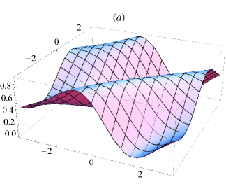
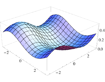
Figure 1: Representations of $(1+\beta\cos(x_{1}))(1+\beta\cos(x_{2}))(1+\beta\cos(x_{1}-x_{2}))$ for $\beta=i$.  $(a)$ Exactly two sheets with $Y_{2}/Y_{1}=\sqrt{2}$ and $Y_{2}=3.87$. The function $Q_{+}({\bm{x}})$ is displayed.  $(b)$ Four sheets with $Y_{1},Y_{2}=\pm Y$ and $Y=1.51$. The function $Q_{++}({\bm{x}})$ is displayed.

The $Q_{\bm{\sigma}}$ will be non negative for $Y>Y_{c}$, with $Y_{c}$ obtained from the condition

$$\sum_{{\bm{\sigma}}}q_{\bm{\sigma}}=-1,\qquad q_{\bm{\sigma}}\equiv\min_{{\bm{x}}}(Q_{\bm{\sigma}}({\bm{x}})-N_{\bm{\sigma}})\,.$$ (37)

As illustration, consider the two-dimensional distribution

$$P(x_{1},x_{2})\propto(1+\beta\cos(x_{1}))(1+\beta\cos(x_{2}))(1+\beta\cos(x_{1}-x_{2})),$$ (38)

with $\beta=i$. This distribution admits a positive representation using exactly two sheets with an asymmetric choice ${\bm{Y}}\propto(1,\sqrt{2})$. The relation $Q_{-}({\bm{x}})=Q_{+}(-{\bm{x}})$ holds automatically. The optimal width, that is, such that $\min_{{\bm{x}}}Q_{+}({\bm{x}})=0$, is obtained as $\,{\bm{Y}}=(2.74,3.87)$. The branch $Q_{+}({\bm{x}})$ is displayed in Fig. 1$a$.

The alternative construction with four sheets, $Q_{\pm\pm}({\bm{x}})$, attains a positive representation with $\,{\bm{Y}}=(\pm 1.51,\pm 1.51)$, which having a smaller width represents an improvement over the previous asymmetric construction. Symmetry under $(x_{1},x_{2})\to(x_{2},x_{1})$ is automatic, and also $Q_{-\mp}({\bm{x}})=Q_{+\pm}(-{\bm{x}})$ is fulfilled. The branch $Q_{++}({\bm{x}})$ is displayed in Fig. 1$b$, the branch $Q_{+-}({\bm{x}})$ has a similar shape, up to a reflection.

III.3 Representations from convolutions

The representations just described can be written as convolutions. Let us consider first the simple case in which problems coming from ${\bm{k}}\cdot{\bm{Y}}=0$ can be neglected. The zero mode is treated separately as this singular term is always present. Straightforward reconstruction of the Fourier sum using the components in Eq. (33) gives

$$Q_{+}({\bm{x}})=N_{+}+2\mathrm{Re}\sum_{{\bm{k}}\not=0}\frac{e^{i{\bm{k}}\cdot{\bm{x}}}e^{{\bm{k}}\cdot{\bm{Y}}}}{2\sinh(2{\bm{k}}\cdot{\bm{Y}})}\int\frac{d^{n}x^{\prime}}{(2\pi)^{n}}e^{-i{\bm{k}}\cdot{\bm{x}}^{\prime}}P({\bm{x}}^{\prime}).$$ (39)

In order to proceed, let us introduce the following function

$$\chi(\Omega)\equiv\frac{\Omega}{\Omega^{2}-\Omega^{-2}}$$ (40)

and also the distribution

$$C({\bm{x}};{\bm{Y}})\equiv\sum_{{\bm{k}}\not=0}e^{i{\bm{k}}\cdot{\bm{x}}}\chi(e^{{\bm{k}}\cdot{\bm{Y}}}).$$ (41)

This allows to express $Q_{\pm}({\bm{x}})$ as convolutions:

$$\begin{split}Q_{\pm}({\bm{x}})&=N_{\pm}+2\mathrm{Re}(C({\bm{x}};\pm{\bm{Y}})*P({\bm{x}}))\\ &=N_{\pm}+2\mathrm{Re}(C(\pm{\bm{x}};{\bm{Y}})*P({\bm{x}})).\end{split}$$ (42)

(For convenience we denote $f(x)*g(x)$ what is usually denoted $(f*g)(x)$.) As is readily verified, the identities

$$\begin{split}&\chi(\Omega)\Omega+\chi(\Omega^{-1})\Omega^{-1}=1,\\ &\chi(\Omega)\Omega^{-1}+\chi(\Omega^{-1})\Omega=0,\end{split}$$ (43)

guarantee the fulfillment of Eq. (32). It should be noted that the expression using real part in Eq. (42) refers only to real ${\bm{x}}$. Of course the analytic extension implied in Eq. (32) has to be applied after the real part is expanded in Eq. (42) as a linear combination of $P({\bm{x}})$ and $P^{*}({\bm{x}})$.

We can turn now to the improved construction using $2^{n}$ branches. Again the zero mode is treated separately, only subject to the conditions

$$1=\sum_{\bm{\sigma}}N_{\bm{\sigma}},\qquad N_{\bm{\sigma}}\geq 0.$$ (44)

For the remaining Fourier modes the expression in Eq. (39) still holds with ${\bm{Y}}=Y{\bm{\sigma}}$ and taking into account that not all modes contribute to each branch ${\bm{\sigma}}$: In principle, a given mode ${\bm{k}}=(k_{1},\ldots,k_{n})$ contributes only to the branch with all $\sigma_{i}$ equal to $\,{\mathrm{sign}}(k_{i})$ or all opposite. When some $k_{i}$ are zero, these are equally distributed between the $\sigma_{i}=1$ and $\sigma_{i}=-1$ options.

In this way, the functions $Q_{\bm{\sigma}}({\bm{x}})$ can be written as convolutions in the form

$$Q_{\bm{\sigma}}({\bm{x}})=N_{\bm{\sigma}}+2\mathrm{Re}(C({\bm{\sigma}}*{\bm{x}};Y)*P({\bm{x}})),\quad{\bm{\sigma}}=(\pm,\ldots,\pm),$$ (45)

where we have defined

$${\bm{\sigma}}*{\bm{x}}\equiv(\sigma_{1}x^{1},\ldots,\sigma_{n}x^{n}),$$ (46)

and

$$C({\bm{x}};Y)\equiv\sum_{\bm{k}}e^{i{\bm{k}}\cdot{\bm{x}}}\chi(e^{Y\sum_{i}k_{i}})\,\Theta({\bm{k}}).$$ (47)

The function $\Theta({\bm{k}})$ selects the Fourier modes contributing to the branch $(+,\ldots,+)$,

$$\Theta({\bm{k}})\equiv\left\{\begin{matrix}\prod_{i=1}^{n}\theta(k_{i})+\prod_{i=1}^{n}\theta(-k_{i})&({\bm{k}}\not=0)\\ 0&({\bm{k}}=0)\end{matrix}\right.,$$ (48)

$\theta(x)$ being the Heaviside step function with $\theta(0)=1/2$. The function $\Theta({\bm{\sigma}}*{\bm{k}})$ does the same job for a branch ${\bm{\sigma}}$.

III.4 Complex representations and linearity

III.4.1 The projection operator $K$

Loosely speaking, a (in general complex) distribution $\rho$ on the complexified manifold defines, through Eq. (2), an associated complex probability $P$ on the real manifold. Let us denote by $K$ the corresponding projection operator, that is,

$$K\rho=P.$$ (49)

Of course, as for the observables, this assumes some class of sufficiently well behaved $\rho$.

To make precise definitions, let us consider a periodic setting in one dimension, hence the real manifold is the circle $\mathrm{S}^{1}\cong[0,2\pi]$ and the complex manifold is the cylinder $\mathrm{S}^{1}\times\mathbb{R}$. As space of test functions on the cylinder, $A(z)$, let us take the linear span of the Fourier modes $e^{ikz}$, this space will be denoted ${\mathcal{D}}_{c}$. The space of densities $\rho(z)$ can be chosen in many ways. A sufficiently general space is that of Schwartz distributions on the cylinder and with bounded support in it. Let us denote this space ${\mathcal{R}}$. Then $\rho$ defines a linear form $\tilde{\rho}\in{\mathcal{D}}_{c}^{*}$ (where ${\mathcal{D}}_{c}^{*}$ denotes the algebraic dual of ${\mathcal{D}}_{c}$) by means of

$$\langle\tilde{\rho},A\rangle\equiv\langle A\rangle_{\rho}.$$ (50)

(We have used the notation $\langle T,f\rangle$ to denote the action of a linear form $T$ on a vector $f$.) It should be clear that the linear map $\hat{\pi}:\rho\to\tilde{\rho}$ from ${\mathcal{R}}\to{\mathcal{D}}_{c}^{*}$ is not one-to-one, as there are many different $\rho$ yielding precisely the same expectation values, and so the same linear map $\tilde{\rho}$.

Next, we can define the space ${\mathcal{D}}_{r}$ as the span of Fourier modes $e^{ikx}$ on $\mathrm{S}^{1}$. Clearly the analytic continuation operator ${\mathcal{A}}$ is an isomorphism of vector spaces from ${\mathcal{D}}_{r}$ to ${\mathcal{D}}_{c}$, namely, $A_{c}={\mathcal{A}}A_{r}$, with $A_{r}(x)=\sum_{k}a_{k}e^{ikx}$ and $A_{c}(z)=\sum_{k}a_{k}e^{ikz}$. Therefore, the dual spaces ${\mathcal{D}}_{r}^{*}$ and ${\mathcal{D}}_{c}^{*}$ are equally isomorphic. $P\in{\mathcal{D}}_{r}^{*}$ can then be defined as the linear form on ${\mathcal{D}}_{r}$ matching $\tilde{\rho}$:

$$\langle\tilde{\rho},{\mathcal{A}}A_{r}\rangle=\langle P,A_{r}\rangle\qquad\forall A_{r}\in{\mathcal{D}}_{r},$$ (51)

that is, $P={\mathcal{A}}^{T}\tilde{\rho}$. The operator $K$, such that $P=K\rho$, is then well-defined, and can be expressed as $K={\mathcal{A}}^{T}\hat{\pi}$.

It is noteworthy that even though $\rho$ is a distribution on the cylinder $\mathrm{S}^{1}\times\mathbb{R}$, the linear form $P$ needs not be a distribution (i.e., a continuous linear form) on the circle $\mathrm{S}^{1}$. For instance, $\rho(z)=\delta(z-z_{0})$ (a two-dimensional Dirac delta) has expectation values $\langle e^{ikz}\rangle_{\rho}=e^{ikz_{0}}$ and these are the Fourier components of $P(x)$. When ${\,{\mathrm{Im}}\,z}_{0}\neq 0$ they are not polynomially bounded, hence $P$ is not a Schwartz distribution on $\mathrm{S}^{1}$. A simple way to choose the space ${\mathcal{R}}$ so that the $P$ are bounded linear forms is to keep only the $\rho$’s which contain a finite number of Fourier modes (with respect to $x\in\mathrm{S}^{1}$), each mode weighted with a Schwartz distributions of bounded support with respect to the variable $y$, i.e., $\rho=\sum_{k}\rho_{k}(y)e^{ikx}$ (a finite sum and $\rho_{k}(y)$ of bounded support).

We have spelled out the definition of the operator $K$ in the setting of periodic one-dimensional functions. Clearly the analogous constructions can be carried out for more general compact groups using a decomposition in terms of irreducible representations.

For sufficiently well behaved distributions $\rho$ on $\mathbb{C}^{n}$ the action of $K$ can be simply expressed as Okano:1992hp ; Salcedo:1993tj

$$P({\bm{x}})=\int d^{n}y\,e^{-i\,{\bm{y}}\cdot{\bm{\nabla}}_{x}}\rho({\bm{x}},{\bm{y}})\equiv\int d^{n}y\,\rho({\bm{x}}-i{\bm{y}},{\bm{y}}).$$ (52)

This is a straightforward consequence of $\langle A(x+iy)\rangle_{\rho}=\langle A(x)\rangle_{P}$ for all $A$. Eq. (32) illustrates this relation when $\rho({\bm{z}})$ has the two-branch form in Eq. (31).

III.4.2 Construction of real representations from linearity

Let us assume that a complex density $P$ can be expressed as a linear combination of some other densities $P_{i}$

$$P=\sum_{i}a_{i}P_{i},$$ (53)

where the $a_{i}$ are some complex coefficients, with $\sum_{i}a_{i}=1$ if $P$ and the $P_{i}$ should be normalized. To avoid any convergence issues we assume the collection $\{P_{i}\}$ to be finite. If each $P_{i}$ admits a real representation $\rho_{i}$, $P_{i}=K\rho_{i}$, due to linearity of $K$, the distribution

$$\rho_{c}\equiv\sum_{i}a_{i}\rho_{i}$$ (54)

will be a representation of $P$, i.e., $P=K\rho_{c}$. Unfortunately, even if all the $\rho_{i}$ a real, such $\rho_{c}$ will be complex in general since the $a_{i}$ are complex.

Abstracting what has been implicitly done in the previous subsections, in order to obtain a real representation one can proceed as follows.

First, the constant mode is treated separately and added a posteriori. So we consider here complex distributions with zero normalization: $P=\sum_{i}a_{i}P_{i}$ where the $P_{i}$, and hence $P$, integrate to zero.

Next, $K$ is a linear operator. Let us introduce the anti-analytic version of $K$, which will be denoted by $\bar{K}$ and is also linear, through the relation

$$\bar{K}\rho=(K\rho^{*})^{*}.$$ (55)

Now given a collection of complex densities $P_{i}(x)$ we associate a set of complex representations $\hat{\rho}_{i}(z)$ subject to the two (linear) requirements

$$P_{i}=K\hat{\rho}_{i},\qquad 0=\bar{K}\hat{\rho}_{i}.$$ (56)

That is, the analytic projections of the $\hat{\rho}_{i}$ yield $P_{i}$ (i.e., the $\hat{\rho}_{i}$ are representations of $P_{i}$ albeit complex) while their anti-analytic projections vanish. Then, obviously

$$\hat{\rho}\equiv\sum_{i}a_{i}\hat{\rho}_{i}$$ (57)

is also a (complex) representation of $P$, i.e., $P=K\hat{\rho}$.

The second equation in (56) is equivalent to

$$0=K\hat{\rho}_{i}^{*}.$$ (58)

Hence $0=K\hat{\rho}^{*}$, and

$$\rho\equiv{\hat{\rho}}+{\hat{\rho}}^{*}=2\mathrm{Re}({\hat{\rho}})$$ (59)

is, by construction, a real representation of $P$,

$$P=K\rho.$$ (60)

To finish the construction, the constant mode should be added to have properly normalized distributions. Because the normalization of $P$ is real, its constant mode, $P_{0}=1$, is real and it can be represented by a real $\rho_{0}$ which is added to ${\hat{\rho}}+{\hat{\rho}}^{*}$.

The two-branch construction follows the scheme of Eqs. (56) and these equations admit many more solutions for a given collection $\{P_{i}\}$. It is interesting that unlike $\rho$, the complex representations $\hat{\rho}$ or $\hat{\rho}_{i}$ preserve information on the phases of $P$ and $P_{i}$, respectively. This implies that one can make new linear recombinations as long as the complex representations are retained. This is no longer possible after the real part operation is applied to obtain a real representation.

Another remark is that if $P_{i}$ has some symmetry, one can impose the same symmetry on its complex representation $\hat{\rho}_{i}$, so each symmetry type (irreducible representation of the symmetry group) can be represented independently, thanks to the linearity of the construction.

The adaptation of this construction to the noncompact case deserves a separate discussion. The expression in Eq. (24) holds equally well for a normalized complex probability $P(x)$ defined on $\mathbb{R}$, using the Fourier components $\tilde{P}(k)$ there,

$$P(x)=\int\frac{dk}{2\pi}\,e^{ikx}\tilde{P}(k),\qquad\int dx\,P(x)=1.$$ (61)

The $k\to 0$ limits of $\tilde{Q}_{\pm}(k)$ in Eq. (24) exist, since $\tilde{P}(0)$ is a real number. As a consequence $\tilde{Q}_{\pm}(0)$ take well defined values, rather than being free parameters as in the compact case.

The functions $Q_{\pm}(x)$ receive (linear) contributions from $P(x)$ and $P^{*}(x)$, and we can denote $\hat{Q}_{\pm}(x)$ the component coming only from $P$ (analogous to $\hat{\rho}$, as compared to $\rho={\hat{\rho}}+{\hat{\rho}}^{*}$). In this case one finds that the Fourier modes

$$\hat{\tilde{Q}}_{\pm}(k)=\pm\frac{e^{\pm kY}}{2\sinh(2kY)}\tilde{P}(k),$$ (62)

display a pole at $k=0$. This implies that the complex representations $\hat{Q}_{\pm}(x)$ are not convergent at infinity. More precisely, their real parts, $Q_{\pm}(x)$, are convergent but their imaginary parts are not.

In general, in the noncompact case, complex representations ${\hat{\rho}}_{i}$ corresponding to normalized $P_{i}$, will produce complex combinations $\sum_{i}a_{i}\hat{\rho}_{i}$ which will not be properly convergent, however, the divergence cancels in their real parts provided the normalization $\sum_{i}a_{i}$ is a real number.

Let us note that the infrared divergence must necessarily be present in $\hat{\rho}$ (this is clear in Eq. (62), since $\tilde{P}(0)=1$). This comes from a conflict in Eq. (56) in the noncompact case. In the compact case, the constant mode was cleanly separated and all distributions in Eq. (56) were assumed to have zero normalization. The same cannot be done in the noncompact case. If the constant mode cannot be extracted one finds an incompatibility in Eq. (56). To see this let us denote by $\hat{P}_{0}$ and $\hat{P}_{00}$ the operators yielding the normalization of distributions on ${\mathcal{M}}$ and ${\mathcal{M}}^{c}$, respectively ($\hat{P}_{0}=\int dx$ and $\hat{P}_{00}=\int d^{2}z$ for ${\mathcal{M}}=\mathbb{R}$). These operators fulfill the identities

$$\hat{P}_{0}K=\hat{P}_{0}\bar{K}=\hat{P}_{00}.$$ (63)

Applying them to

$$P=K{\hat{\rho}},\qquad 0=\bar{K}{\hat{\rho}}.$$ (64)

one finds

$$1=\hat{P}_{0}P=\hat{P}_{00}{\hat{\rho}},\qquad 0=\hat{P}_{00}{\hat{\rho}}.$$ (65)

The conflict results in a singularity in the imaginary part of ${\hat{\rho}}$ at the constant mode.

IV Localized representations on Lie groups

In this section we aim at extending the previous constructions to non necessarily abelian Lie groups. Eventually we will limit our study to compact groups because too general (group) representations of noncompact groups would be intractable, even qualitatively. Nevertheless, it can be conjectured that our results apply also to a complex probability $P$ defined on any Lie group $G$, provided $P$ is spanned by a set of well behaved representations of $G$ (e.g., bounded representations). The case $G=(\mathbb{R}^{n},+)$ and $P({\bm{x}})$ admitting a Fourier decomposition in terms of $e^{i{\bm{k}}\cdot{\bm{x}}}$, for ${\bm{k}}\in\mathbb{R}^{n}$ (as opposed to ${\bm{k}}\in\mathbb{C}^{n}$) is such an example.

IV.1 Representations on groups

For definiteness we will assume a connected matrix group,

$$G=\{\,g({\bm{a}})=e^{\,{\bm{a}}\cdot{\bm{T}}},~{}{\bm{a}}\in\mathbb{R}^{n}\,\},$$ (66)

where the matrices $\,T_{i}~{}(i=1,\ldots,n)$ are the group generators and $a^{i}~{}(i=1,\ldots,n)$ are the normal coordinates of the element $g$. New admissible real coordinate systems are derived by means of real analytic changes of variables.

The complexified group $G^{c}$ is obtained by taking complex values for the coordinates,

$$G^{c}=\{\,g({\bm{a}})=e^{\,{\bm{a}}\cdot{\bm{T}}},~{}{\bm{a}}\in\mathbb{C}^{n}\,\}.$$ (67)

The analytically extended observables are defined on $G^{c}$ through analytic extension with respect to their dependence on the coordinates. (The extension does not depend on the concrete coordinates used as long as they belong to the class of admissible ones.)

Given a positive measure $d\mu(g)$ on $G$, one can define complex distributions $P(g)$ on $G$ and corresponding expectation values. The factor between two different choices of measure can be reabsorbed in the distribution, so without loss of generality, we will use the right-invariant Haar measure of $G$. For compact $G$ we adopt the normalized measure

$$\int_{G}dg=1\quad\text{(compact~{}$G$)}\,.$$ (68)

Likewise, we take the right-invariant measure on $G^{c}$. The complexified group is never compact, but will be unimodular if $G$ is. The concept of representation works as before, as dictated by Eq. (2).

We will need to introduce the (complex) conjugate element $\bar{g}$ of a given $g\in G^{c}$. This is defined by

$$g=g({\bm{a}}),\qquad\bar{g}=g({\bm{a}}^{*})\qquad{\bm{a}}\in\mathbb{C}^{n}.$$ (69)

This conjugation is a group automorphism in $G^{c}$ and its definition does not depend on the particular coordinates used in $G$. Also note that $\bar{g}$ needs not coincide with $g^{*}$ (the conjugate matrix in a matrix group) unless ${\bm{T}}^{*}={\bm{T}}$.

An important property of the conjugation is that, for any (group) representation $D(g)$ of $G$ and $D^{*}(g)=D(g)^{*}$ its conjugate representation, upon analytic extension into $G^{c}$,

$$(D(g))^{*}=D^{*}(\bar{g})\qquad g\in G^{c}.$$ (70)

Obviously, the set of autoconjugated (real) elements is $G$ itself,

$$g=\bar{g}\quad\text{iff}\quad g\in G.$$ (71)

The subset of purely imaginary elements of $G^{c}$, which we denote $G_{I}$, can be naturally defined as

$$g\in G_{I}\quad\text{iff}\quad\bar{g}=g^{-1}.$$ (72)

In normal coordinates $G_{I}$ are those elements of $G^{c}$ with purely imaginary coordinates. In the non abelian case $G_{I}$ is not a subgroup of $G^{c}$, however if $g\in G$, $\,gG_{I}g^{-1}=G_{I}$. Also, if $h\in G_{I}$, $h^{s}\in G_{I}$, for $s\in\mathbb{R}$. Furthermore, $G^{c}=GG_{I}=G_{I}G$.

IV.2 Two-branch representations

We will not need very general distributions on $G^{c}$, rather we use a two-branch approach (with suitable variations in the higher dimensional case, as in Sec. III.2.2). That is, for a given (normalized) complex probability $P(g)$

$$1=\int_{G}dg\,P(g),$$ (73)

we seek two positive distributions $Q_{\pm}(g)$ on $G$ in such a way that they define a representation of $P(g)$, by means of the relation, analogous to (32),

$$P(g)=Q_{+}(gg_{+})+Q_{-}(gg_{-})\qquad\forall g\in G,$$ (74)

where $g_{\pm}\in G^{c}$ are two parameters of the construction, and $Q_{\pm}(gg_{\pm})$ refer to the analytic extension of $Q_{\pm}(g)$ into the complexified group. Indeed, using the right-invariance of the measure,

$$\begin{split}\langle A\rangle_{P}&=\int_{G}dg\,A(g)P(g)=\int_{G}dg\,A(g)\sum_{\sigma=\pm}Q_{\sigma}(gg_{\sigma})\\ &=\int_{G}dg\sum_{\sigma=\pm}Q_{\sigma}(g)\,A(gg_{\sigma}^{-1})\\ &=N_{+}\langle A(gg_{+}^{-1})\rangle_{Q_{+}}+N_{-}\langle A(gg_{-}^{-1})\rangle_{Q_{-}},\end{split}$$ (75)

where $N_{\pm}$ denote the normalizations of $Q_{\pm}$,

$$N_{\pm}=\int_{G}dg\,Q_{\pm}(g),$$ (76)

with

$$1=N_{+}+N_{-},\quad N_{\pm}\geq 0.$$ (77)

Eq. (75) implies that the expectation value of $A$ can be obtained by importance sampling of the two positive distributions $Q_{\pm}(g)$ defined on $G$. The representation $\rho(g)$ itself has support on two copies of $G$ contained in $G^{c}$, namely, $Gg_{+}^{-1}$ and $Gg_{-}^{-1}$. Therefore the elements $g_{\pm}$ represent the displacements away from $G$ into $G^{c}$.

In Eq. (74) we have arbitrarily chosen the shift to act on the right. Of course everything would be analogous with $Q_{+}(g_{+}g)+Q_{-}(g_{-}g)$. Also possible would be (for a unimodular group)

$$P(g)=Q_{+}(g^{\prime}_{+}gg_{+})+Q_{-}(g_{-}^{\prime}gg_{-}).$$ (78)

We do not explore this latter possibility as it is technically more complicated with no obvious advantage.

It is clear that there is no solution to Eq. (74) (with positive $Q_{\pm}$) if $g_{\pm}\in G$, unless $P$ is already a positive distribution. As discussed in Sec. II.3, the representation $\rho(g)$ must have some support sufficiently far from the real manifold (the group $G$ in this case); a minimal width is required for any positive representation $\rho$.

The complex distribution $P$ is equivalent (has the same information as) to two real functions, so it can be expected that for given $g_{\pm}$, the two real functions $Q_{\pm}$ are essentially unique. To actually determine the two branches $Q_{\pm}$ we apply the approach developed in Sec. III.4.2 as follows.

The (group) representations of a group span the space of complex functions defined on that group (i.e., its regular representation Barut:1986dd ). So general distributions $P(g)$ can be expanded as linear combinations of (group) representations $D^{R}(g)$ of $G$, i.e., $P(g)\sim\sum_{R}P^{R}D^{R}(g)$.

In order to cleanly separate the normalization mode (constant mode) in $P$, we will assume in what follows that $G$ is a compact group, hence our complex normalized probability $P(g)$ can be expressed as

$$\begin{split}P(g)&=1+\sum_{R\not=1}\sum_{\alpha,\beta}(P^{R}){}^{\beta}{}_{\alpha}\,D^{R}(g)^{\alpha}{}_{\beta}\\ &=1+\sum_{R\not=1}{\mathrm{tr}}(P^{R}\,D^{R}(g)).\end{split}$$ (79)

The $P^{R}$ are constant complex matrices of the same dimension as the representation $R$. We have separated the trivial (or singlet) representation $D^{R=1}(g)\equiv 1$ which must carry weight $1$ if $P$ is normalized.

As follows from the Peter-Weyl theorem, the set of irreducible representations (irreps) form an orthonormal basis for the regular representation and we could take the $R$ to be irreducible, however, such assumption is not strictly needed for our construction, so we will only assume that $R$ does not contain the trivial representations in its decomposition into irreps, therefore

$$\int_{G}dg\,D^{R}(g)=0\qquad(R\not=1).$$ (80)

To apply the scheme of Sec. III.4.2, we will seek complex representations for each component $R$ in $P$, fulfilling the conditions in Eqs. (56). That is, for each $R\not=1$ we seek two functions $\hat{Q}^{R}_{\pm}(g)$ of the form

$$\hat{Q}^{R}_{\pm}(g)={\mathrm{tr}}(Q^{R}_{\pm}\,D^{R}(g)),$$ (81)

where $Q^{R}_{\pm}$ are two matrices to be determined. Then the real distributions

$$Q^{R}_{\pm}(g)=2\mathrm{Re}\,\hat{Q}^{R}_{\pm}(g)\qquad g\in G$$ (82)

are the two real branches in the representation of the component $R$ of $P(g)$ and

$$Q_{\pm}(g)=N_{\pm}+\sum_{R\not=1}Q^{R}_{\pm}(g).$$ (83)

The two functions $\hat{Q}^{R}_{\pm}(g)$ are to be determined through Eq. (56). The action of the operator $K$ in our case can be read off from Eq. (74) since that equation is just $P=K\rho$.

The representation condition on $\hat{Q}^{R}_{\pm}(g)$ (first relation in Eq. (56)) becomes (using Eq. (81))

$$\begin{split}{\mathrm{tr}}(P^{R}D^{R}(g))&=\sum_{\sigma=\pm}\hat{Q}^{R}_{\sigma}(gg_{\sigma})=\sum_{\sigma=\pm}{\mathrm{tr}}(Q^{R}_{\sigma}\,D^{R}(g)D^{R}(g_{\sigma})),\end{split}$$ (84)

that is

$$P^{R}=D^{R}(g_{+})\,Q^{R}_{+}+D^{R}(g_{-})\,Q^{R}_{-}.$$ (85)

To impose the second relation in Eq. (56), note that

$$\hat{Q}^{R}_{\pm}(g)^{*}={\mathrm{tr}}(Q^{R}_{\pm}{}^{*}\,D^{R*}(g)),\quad g\in G,$$ (86)

where $D^{R*}$ is the conjugate representation of $D^{R}$. Then Eq. (58) takes the form

$$0=\sum_{\sigma=\pm}{\mathrm{tr}}\left(Q^{R}_{\sigma}{}^{*}\,D^{R*}(g)\,D^{R*}(g_{\sigma})\right).$$ (87)

Taking complex conjugation and using Eq. (70) yields

$$0=\sum_{\sigma=\pm}{\mathrm{tr}}\left(Q^{R}_{\sigma}\,D^{R}(g)D^{R}(\bar{g}_{\sigma})\right),$$ (88)

which provides a second equation on $Q^{R}_{\pm}$:

$$0=D^{R}(\bar{g}_{+})\,Q^{R}_{+}+D^{R}(\bar{g}_{-})\,Q^{R}_{-}.$$ (89)

Assuming that the required matrices are invertible, the system of Eqs. (85) and (89) can be solved to give

$$Q^{R}_{\pm}=\left(D^{R}(g_{\mp}^{-1}g_{\pm})-D^{R}(\bar{g}_{\mp}^{-1}\bar{g}_{\pm})\right)^{-1}D^{R}(g_{\mp}^{-1})\,P^{R}.$$ (90)

Equivalently,

$$Q^{R}_{\pm}=\left(1-D^{R}(g_{\pm}^{-1}g_{\mp}\bar{g}_{\mp}^{-1}\bar{g}_{\pm})\right)^{-1}D^{R}(g_{\pm}^{-1})\,P^{R}.$$ (91)

So a solution is obtained whenever the matrix $D^{R}(g_{\pm}^{-1}g_{\mp}\bar{g}_{\mp}^{-1}\bar{g}_{\pm})$ has no eigenvalue $\lambda=1$. If it has, there can still be solutions if $P$ has no component along those eigenvectors. We come back to this crucial question in Sec. V. For the time being we will assume that the required matrices are indeed invertible. As always the trivial representation (constant mode) has been explicitly extracted (since certainly all eigenvalues $\lambda=1$ when $R=1$).

As noted $G^{c}=GG_{I}$. Since the factors of $g_{\pm}$ along $G$ are ineffective, the most efficient choice, in principle, corresponds to taking purely imaginary displacements. Hereafter we adopt this prescription, $g_{\pm}\in G_{I}$, and also choose a symmetric disposition of the two shifts, $g_{+}=g_{-}^{-1}$:

$$h\equiv g_{+}=g_{-}^{-1}=\bar{g}_{+}^{-1}=\bar{g}_{-}\in G_{I}.$$ (92)

Then Eq. (74) becomes

$$P(g)=Q_{+}(gh)+Q_{-}(gh^{-1})\qquad\forall g\in G,$$ (93)

and

$$\langle A\rangle_{P}=N_{+}\langle A(gh^{-1})\rangle_{Q_{+}}+N_{-}\langle A(gh)\rangle_{Q_{-}}.$$ (94)

Also Eqs. (85) and (89) become

$$\begin{split}P^{R}&=D^{R}(h)\,Q^{R}_{+}+D^{R}(h^{-1})\,Q^{R}_{-}\\ 0&=D^{R}(h^{-1})\,Q^{R}_{+}+D^{R}(h)\,Q^{R}_{-}\end{split}\,.$$ (95)

In addition Eq. (90) becomes

$$Q^{R}_{+}=\chi(D^{R}(h))\,P^{R},\quad Q^{R}_{-}=\chi(D^{R}(h^{-1}))\,P^{R},$$ (96)

where $\chi$ is the function introduced in Eq. (40) and $\chi(D^{R}(h))$ is a matrix of the same dimension as $R$. Therefore, the two branches for the representation of $P(g)$ can be compactly written as

$$Q_{\pm}(g)=N_{\pm}+2\mathrm{Re}\sum_{R\not=1}{\mathrm{tr}}\!\left[P^{R}\,D^{R}(g)\,\chi(D^{R}(h^{\pm 1}))\right].$$ (97)

Because $G$ is compact and its representations $R$ are unitary, the matrices $D^{R}(g)$ are unitary, while $D^{R}(h)$ (and hence $\chi(D^{R}(h))$) are hermitian. This follows from the identity

$$D^{R}(g^{-1})=D^{R}(g)^{-1}=D^{R}(\bar{g})^{\dagger}\quad\forall g\in G^{c}\quad\text{($R$ unitary)}.$$ (98)

Once again, for sufficiently large $h$ (assuming no $\lambda=1$ eigenvalues are involved) $\chi(D^{R}(h))$ goes to zero and only the singlet (trivial representation) mode remains in Eq. (97), implying that eventually $Q_{\pm}$ become non negative.

Of course the case $G=\mathrm{U}(1)^{\times n}$ studied in Sec. III conforms to this general scheme: the normal coordinates are ${\bm{a}}={\bm{x}}$ in $G$ and ${\bm{a}}={\bm{z}}$ in $G^{c}=(\mathrm{U}(1)\times\mathbb{R})^{\times n}$. Also, $R={\bm{k}}$, $D^{R}(g)=e^{i{\bm{k}}\cdot{\bm{x}}}$ and $P^{R}=\tilde{P}_{\bm{k}}$. Furthermore, $h$ has coordinates $-i{\bm{Y}}$ and so $D^{R}(h)=e^{\,{\bm{k}}\cdot{\bm{Y}}}$. In this way Eq. (97) reproduces Eq. (39).

IV.3 An $\mathrm{SU}(2)$ example

Let us consider the following complex probability on $G=\mathrm{SU}(2)$

$$P(g)=1+{\mathrm{tr}}(pg)\,\quad g\in\mathrm{SU}(2).$$ (99)

Here $p$ is a constant complex $2\times 2$ matrix. Letting $h\in\mathrm{SU}(2)_{I}$, a direct application of the previous results gives

$$Q_{\pm}(g)=N_{\pm}\pm 2\mathrm{Re}\,{\mathrm{tr}}\left(h^{\pm 1}(h^{2}-h^{-2})^{-1}pg\right).$$ (100)

To be more explicit, let

$$\begin{split}g&=\cos(\psi/2)-i\sin(\psi/2)\,\hat{\bm{\psi}}\cdot{\bm{\sigma}},\\ p&=p_{0}+{\bm{p}}\cdot{\bm{\sigma}},\\ h&=\cosh(Y)+\sinh(Y)\,\hat{\bm{Y}}\cdot{\bm{\sigma}},\end{split}$$ (101)

where $p_{0}$ and ${\bm{p}}$ can be complex and ${\bm{\psi}}$ and ${\bm{Y}}$ are real. Then

$$Q_{\pm}(g)=A_{\pm}a_{0}+{\bm{B}}_{\pm}\cdot{\bm{a}}$$ (102)

with

$$a_{0}=\cos(\psi/2),\quad{\bm{a}}=\sin(\psi/2)\hat{\bm{\psi}}$$ (103)

and

$$\begin{split}A_{\pm}&=\frac{\mathrm{Re}(p_{0})}{\cosh(Y)}\pm\frac{\hat{\bm{Y}}\cdot\mathrm{Re}({\bm{p}})}{\sinh(Y)}\\ {\bm{B}}_{\pm}&=\pm\frac{\hat{\bm{Y}}\,{\,{\mathrm{Im}}\,(}p_{0})}{\sinh(Y)}\pm\frac{\hat{\bm{Y}}\times\mathrm{Re}({\bm{p}})}{\sinh(Y)}+\frac{{\,{\mathrm{Im}}\,(}{\bm{p}})}{\cosh(Y)}.\end{split}$$ (104)

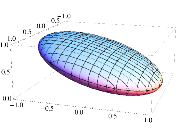
Figure 2: For $g\in\mathrm{SU}(2)$, function $Q_{+}(g)$ on the plane $(a_{1},a_{3})$ with $a_{2}=0$, for $P(g)=1+\beta\,{\mathrm{tr}}(g)$ with $\beta=1-i$, and $h={\rm diag}(e^{Y},e^{-Y})$ with $Y=3.5$, and $N_{+}=1/2$.

As an illustration, in Fig. 2 we show the function $Q_{+}(g)$ for

$$P(g)=1+\beta\,{\mathrm{tr}}(g),\qquad\beta=1-i,$$ (105)

using $\hat{\bm{Y}}=(0,0,1)$ and $Y=3.5$, and $N_{+}={\textstyle{\frac{1}{2}}}$. $\mathrm{SU}(2)$ is a three-sphere, $a_{0}^{2}+{\bm{a}}^{2}=1$, so $Q_{+}$ as a function of ${\bm{a}}$ is two-valued. The plot displays $Q_{+}(a_{1},0,a_{3})$, the submanifold $a_{2}=0$ being a two-sphere.

It is interesting to note that in any $\mathrm{U}(N)$ group the complex probabilities of the type in Eq. (99) can be reduced to a standard form before representation. The matrix $p$ can be written as

$$p=u_{L}du_{R},\quad u_{L,R}\in\mathrm{U}(N),\quad d~{}\text{diagonal and non negative},$$ (106)

so that

$$P(g)=1+{\mathrm{tr}}(du_{R}gu_{L}).$$ (107)

Then it is sufficient to find representations $\rho^{\prime}(g)$ for

$$P^{\prime}(g)=1+{\mathrm{tr}}(dg),$$ (108)

and afterwards undo the left and right translations

$$\rho(g)=\rho^{\prime}(u_{R}gu_{L}).$$ (109)

In the case of $\mathrm{SU}(N)$,

$$p=e^{i\varphi}u_{L}du_{R},\quad u_{L,R}\in\mathrm{SU}(N),\quad d~{}\text{diagonal and non negative}.$$ (110)

($\varphi$ real.) In particular for $\mathrm{SU}(2)$ the most general case required is $p=e^{i\varphi}a(1+\cos\theta\sigma_{3})$, $a>0$,  $\theta,\varphi\in\mathbb{R}$.

IV.4 Representations through convolutions

The functions $Q_{\pm}(g)$ can also be obtained from convolution of $P(g)$ with a fixed kernel. To do this, we express $P$ in terms of irreducible group representations, $\mu$, as

$$\begin{split}P(g)&=\sum_{\mu}{\mathrm{tr}}(P^{\mu}D^{\mu}(g)),\\ P^{\mu}&=n_{\mu}\int_{G}dg\,P(g)\,D^{\mu}(g^{-1}),\end{split}$$ (111)

where $n_{\mu}$ denotes the dimension of the irrep $\mu$. Using the expression of $P^{\mu}$ to work out Eq. (97), one obtains

$$\begin{split}Q_{\pm}(g)&=N_{\pm}+2\mathrm{Re}\int dg^{\prime}\,P(g^{\prime})\,C(g^{\prime}{}^{-1}g\,;\,h^{\pm 1})\\ &=N_{\pm}+2\mathrm{Re}\big{(}P(g)*C(g\,;\,h^{\pm 1})\big{)},\end{split}$$ (112)

with

$$C(g;h)=\sum_{\mu\not=1}n_{\mu}\,{\mathrm{tr}}\big{[}D^{\mu}(g)\,\chi(D^{\mu}(h))\big{]}.$$ (113)

Eqs. (112) and (113) generalize Eqs. (42) and (41), respectively.

Summations on $\mu$ or $\mu^{*}$ (the conjugate irrep) are equivalent within the trace in Eq. (113). Using this rearrangement, along with Eq. (98) and

$$D^{R*}(g)=D^{R}(g^{-1})^{T}\quad\forall g\in G^{c}\quad\text{($R$ unitary)}$$ (114)

one can easily establish the following identities

$$C(g;h^{-1})=C(g^{-1};h)=C(g;h)^{*}.$$ (115)

IV.5 Representations in matrix groups

Let $G\subseteq\mathrm{U}(N)$, and $g^{i}{}_{\!j}$ the matrix elements of $g\in G$  ($i,j=1,\ldots N$). The (group) representations of $G$ can be obtained from tensor product of the basic representations $g$ and $g^{*}$. (Note that such product representations will be reducible in general.)

In the simplest case in which only $g$ is involved

$$P(g)=\sum_{n=0}^{\infty}p^{j_{1}\ldots j_{n}}_{\,i_{1}\ldots\,i_{n}}\,g^{i_{1}}{}_{\!j_{1}}\cdots g^{i_{n}}{}_{\!j_{n}},$$ (116)

where $p^{j_{1}\ldots j_{n}}_{\,i_{1}\ldots\,i_{n}}$ are complex coefficients. This is a decomposition of $P$ into group representations of the type $D^{R}(g)=g\otimes\cdots\otimes g$ ($n$ factors),

$$D^{R}(g)_{j_{1}\ldots j_{n}}^{\,i_{1}\ldots\,i_{n}}=g^{i_{1}}{}_{\!j_{1}}\cdots g^{i_{n}}{}_{\!j_{n}}\equiv(g^{\otimes n})_{j_{1}\ldots j_{n}}^{\,i_{1}\ldots\,i_{n}},$$ (117)

and Eq. (97) applies

$$Q_{+}(g)=N_{+}+2\mathrm{Re}\!\sum_{n=1}^{\infty}\hat{Q}_{n}(g),$$ (118)

with

$$\hat{Q}_{n}(g)=p^{j_{1}\ldots j_{n}}_{\,i_{1}\ldots\,i_{n}}\,(g^{\otimes n})_{k_{1}\ldots\,k_{n}}^{\,i_{1}\ldots\,i_{n}}\,\chi(h^{\otimes n})^{k_{1}\ldots\,k_{n}}_{j_{1}\ldots j_{n}}.$$ (119)

The contribution to $Q_{-}(g)$ is analogous, using $h^{-1}$ instead of $h$. Also note that because $R$ is unitary, $h$ is hermitian.

Let us assume that $h\in G_{I}$ is a diagonal matrix,

$$h={\rm diag}(\omega_{1},\ldots,\omega_{N}).$$ (120)

The $\omega_{\,i}$ are real (and moreover positive for a connected group). In this case $h^{\otimes n}$ and $\chi(h^{\otimes n})$ are also diagonal and $\hat{Q}_{n}(g)$ takes a simple form

$$\hat{Q}_{n}(g)=p^{j_{1}\ldots j_{n}}_{\,i_{1}\ldots\,i_{n}}\,g^{i_{1}}{}_{j_{1}}\cdots g^{i_{n}}{}_{j_{n}}\,\chi(\Omega),\quad\Omega=\omega_{j_{1}}\cdots\omega_{j_{n}}.$$ (121)

$\Omega$ denotes the argument of the function $\chi$ generated by the displacement to the complex manifold. We can see that $\Omega$ picks up a factor $\omega_{j}$ for each factor $g^{i}{}_{j}$ in the representation $R$.

More generally, $R=g^{\otimes n}\otimes g^{*}{}^{\otimes m}$. The corresponding right translation with $h\in G_{I}$ is

$$g\mapsto gh\qquad g^{*}=g^{-1T}\mapsto g^{*}h^{-1T}.$$ (122)

This implies that $\Omega$ picks up a factor $\omega_{j}$ for each factor $g^{i}{}_{j}$ in $R$, and a factor $\omega^{-1}_{j}$ from each factor $g^{*}{}^{i}{}_{j}$. That is, a term

$$P(g)=\,g^{i_{1}}{}_{\!j_{1}}\cdots g^{i_{n}}{}_{\!j_{n}}\,g^{*}{}^{l_{1}}{}_{\!k_{1}}\cdots g^{*}{}^{l_{m}}{}_{\!k_{m}},$$ (123)

gives a contribution

$$\begin{split}\hat{Q}(g)&=\,g^{i_{1}}{}_{\!j_{1}}\cdots g^{i_{n}}{}_{\!j_{n}}\,g^{*}{}^{l_{1}}{}_{\!k_{1}}\cdots g^{*}{}^{l_{m}}{}_{\!k_{m}}\,\chi(\Omega),\\ \Omega&=\omega_{j_{1}}\cdots\omega_{j_{n}}\omega^{-1}_{k_{1}}\cdots\omega^{-1}_{k_{m}}.\end{split}$$ (124)

Similar formulas hold in more general cases. Also note that $g^{\otimes n}$ suffices for $\mathrm{SU}(2)$ since $g$ and $g^{*}=\sigma_{y}g\sigma_{y}$ are equivalent representations in this case.

Another observation is that $\Omega$ may be equal to $1$ for some components and the previous formulas do not directly apply there. This will certainly happen when $R$ contains the trivial representation in its reduction, but not only then. This problem is addressed in Sec. V.

If a configuration of the real manifold consists of $n$ variables, $(\overset{1}{g},\ldots,\overset{n}{g})$, each of them an element of the group $G_{1}\subseteq\mathrm{U}(N)$, the complex probability is defined on the group $G=G_{1}\times\cdots\times G_{1}$ ($n$ factors) and $g=\overset{1}{g}\cdots\overset{n}{g}$. The formulas apply as before, and for instance, a term of the form

$$P(g)=\overset{1}{g}{}^{\,i_{1}}{}_{\!j_{1}}\,\overset{1}{g}{}^{*}{}^{\,i_{2}}{}_{\!j_{2}}\,\overset{2}{g}{}^{\,i_{3}}{}_{\!j_{3}},$$ (125)

with diagonal $h$ with parameters $\overset{r}{\omega}{}_{j}$, would yield a contribution

$$\hat{Q}(g)=\overset{1}{g}{}^{\,i_{1}}{}_{\!j_{1}}\,\overset{1}{g}{}^{*}{}^{\,i_{2}}{}_{\!j_{2}}\,\overset{2}{g}{}^{\,i_{3}}{}_{\!j_{3}}\,\chi(\overset{1}{\omega}{}_{j_{1}}\,\overset{1}{\omega}{}^{-1}_{j_{2}}\,\overset{2}{\omega}{}_{j_{3}}).$$ (126)

It should be noted that a discussion similar to that in Sec. III.2.2 can be (and should be) done here to restore uniformity with respect to the $n$ variables, resulting in a total of $2^{n}$ branches, instead of $2$. An explicit nonabelian example using $2^{n}$ branches is analyzed in Sec. V.3. In the abelian case, bifurcation of the variables solved the problem of singular terms (${\bm{k}}\cdot{\bm{Y}}=0$ denominators). A crucial difference with the abelian case is that the presence of singular components (not invertible matrices in Eq. (97)) is not automatically solved by bifurcation in the nonabelian case, so we defer the discussion to Sec. V.

When the element $h\in G_{I}$ is not directly diagonal but it is diagonalizable within $G$, a practical way to proceed is as follows. Let

$$h=Uh_{z}U^{-1},\qquad U\in G,\quad h_{z}\in G_{I}\text{~{}and diagonal},$$ (127)

and let

$$P^{\prime}(g)\equiv P(Ug\,U^{-1}).$$ (128)

Then

$$\hat{Q}(g)=\hat{Q}^{\prime}(U^{-1}g\,U),$$ (129)

where $\hat{Q}^{\prime}(g)$ is the complex representation associated to $P^{\prime}(g)$, constructed using the diagonal $h_{z}$ as described above. Indeed, using Eq. (97),

$$\begin{split}\hat{Q}(g)&={\mathrm{tr}}\left(P^{R}D^{R}(g)\chi(D^{R}(h))\right)\\ &={\mathrm{tr}}\left(P^{R}D^{R}(g)D^{R}(U)\chi(D^{R}(h_{z}))D^{R}(U)^{-1}\right)\\ &={\mathrm{tr}}\left(P^{\prime}{}^{R}D^{R}(U^{-1}g\,U)\chi(D^{R}(h_{z}))\right)=\hat{Q}^{\prime}(U^{-1}g\,U).\end{split}$$ (130)

V Removal of singular kernels and examples

V.1 Singular kernels

The first expression in Eq. (96) can be rewritten as

$$Q^{R}_{+}=D^{R}(h)^{3}\left(D^{R}(h)^{4}-1\right)^{-1}P^{R}$$ (131)

and similarly for $Q^{R}_{-}$ with $h^{-1}$. Hence there is a proper solution when $D^{R}(h)$ has no $\lambda=1$ eigenvalues or, if it has, $P^{R}$ has no components along the corresponding eigenvectors. Otherwise we meet an obstruction to solving Eq. (95).

As already noted, when a probability $P(g)$ is complex, the support of any of its real representations must necessarily extend beyond $G$ into the complexified manifold. In the two-branch approach the pushing into $G^{c}$ is carried out by $h$ (or more generally $g_{\pm}$). An obstruction arises when some components of $P^{R}$ are not moved by $D^{R}(h)$ (unless they happen to be already positive). The obstruction takes place when some components of $P$ remain invariant under the action of $h$ , i.e., when $h$ does not act effectively on all components of $P$. This is quite clear in the abelian case $\mathrm{U}(1)^{\times n}$ discussed in Sec. III.2.1. There, an obstruction was met for Fourier modes such that ${\bm{k}}\cdot{\bm{Y}}=0$. They correspond to the the Fourier components $e^{i{\bm{k}}\cdot{\bm{x}}}$ of $P$ which remain invariant under the imaginary translation ${\bm{x}}\to{\bm{x}}-i{\bm{Y}}$.

An important observation is that, in the nonabelian case, the obstruction cannot be removed by a clever choice of $h$ (or even $g_{\pm}$ outside $G_{I}$). To see this it suffices to consider the case $G=\mathrm{SU}(2)$. If $R=j$ is a half-integer representation, $D^{j}(h)$ has no eigenvalue equal to $1$, since the operator $J_{z}$ has no zero eigenvalues, and the same is true of $J_{n}=\hat{{\bm{n}}}\cdot{\bm{J}}$; so for those irreps any choice of rotation axis provides a solution. However, for integer $j$, $J_{n}$ has exactly one zero eigenvalue. This means that no matter how the (complex) rotations are chosen $D^{j}(h)$ will have an eigenvalue equal to one for some eigenvector. We conclude that for integer $j$ the obstruction cannot be avoided by just a better choice of the element $h$. For $h$ imaginary the rotation angle is imaginary and the rotation axis $\hat{n}$ is real. Choosing a complex axis would not help though: if $J_{n}$ has a zero eigenvalue whenever $\hat{n}$ is real (and so $\det(\hat{n}\cdot J)=0$) by analytic extension, the zero will persist in the complex case too. Thus we stick to the choice $h\in G_{I}$.

It follows that for certain groups and representations there is no perfect choice of a single $h$ that would work simultaneously for all components of a general complex probability $P$. The obvious solution is to try to decompose $P$ as a sum of terms in such a way that each term can be treated effectively by a different suitable element $h$:

$$P(g)=1+\sum_{k=1}^{m}P_{k}(g)\qquad\text{($h_{k}\in G_{I}$ and acts effectively on $P_{k}$)}.$$ (132)

Eq. (131) would then apply for each term $k=1,\ldots,m$ separately without obstruction, and each $h_{k}$ would introduce a further pair of branches in the support of $\rho$. The arguments given at the end of Sec. III.1 indicate the number $m$ of terms should be as small as possible.

In a setting like that of Eq. (124), i.e., a matrix group with diagonal $h$, the obstruction appears for those components with $\Omega=1$. A simpleminded approach would be to use such diagonal $h$ for the $\Omega\not=1$ terms and a different element $h^{\prime}$ for the remainder. However such strategy is not practical in general. To see this consider again $\mathrm{SU}(2)$ and a representation $R=j$, with integer $j$ (since the half-integer irreps pose no problem). A diagonal $h=h_{z}$ corresponds to a rotation around the $z$ axis. The components in $P$ can be decomposed in the $J_{z}$ basis $|j,m\rangle_{z}$, and $|j,0\rangle_{z}$ will be unaffected by $h_{z}$. A simple prescription is to identify such components from the condition $\Omega=1$. All the $\Omega\not=1$ terms can be treated with $h_{z}$ (of sufficient magnitude to guarantee positivity of the representation). The terms with $\Omega=1$ should be treated with a different element $h_{n}$, corresponding to a rotation around some axis $\hat{\bm{n}}$. As it turns out, one cannot take just any axis. The reason is that we need $h_{n}$ to act effectively on $|j,0\rangle_{z}$: This vector can be decomposed in the basis $|j,m\rangle_{n}$ and one should take $\hat{\bm{n}}$ in such a way that $|j,0\rangle_{z}$ has no component along $|j,0\rangle_{n}$ (since such component would remain unaffected by $h_{n}$). Hence, the axis $\hat{\bm{n}}$ must fulfill the condition

$${}_{z}\langle j,0|j,0\rangle_{n}=0.$$ (133)

In practice, this means that the cosine of the angle between the $z$ axis and $\hat{\bm{n}}$ should be a zero of the $j$-th Legendre polynomial, $P_{j}(\hat{e}_{z}\cdot\hat{{\bm{n}}})=0$. For all odd $j$, ${\bm{n}}=\hat{e}_{x}$ suffices. Unfortunately for even $j$ the axis must be changed for different $j$ and in general an infinite number of branches could be required.

So a method is needed to implement Eq. (132) using a common (and small) set of branches for all representations simultaneously. This can be done as follows.

Let the set of elements $h_{k}\in G_{I}$, $k=1,\ldots,m$, where the number $m$ is to be chosen appropriately for the given group. For any irrep $R\not=1$, let $V^{R}$ be the $n_{R}$-dimensional vector space where $D^{R}(g)$ acts ($n_{R}=\dim R$). Each $h_{k}$ defines a singlet subspace $W^{R}_{k}$ of $V^{R}$ (which may be $\{0\}$); singlet means that within this subspace $h_{k}$ acts as the identity operator:

$$W^{R}_{k}=\{v\in V^{R},\,D^{R}(h_{k})v=v\}.$$ (134)

On the orthogonal complement $W^{R,\perp}_{k}$ the element $h_{k}$ acts effectively [i.e., no non null vector of $W^{R,\perp}_{k}$ is left invariant by $D^{R}(h_{k})$] and

$$V^{R}=W^{R}_{k}\oplus W^{R,\perp}_{k}.$$ (135)

The obstruction is avoided for the irrep $R$ if any vector of $V^{R}$ can be decomposed as a sum where each term is acted effectively by $h_{k}$, i.e.

$$\forall v\in V^{R}\qquad v=\sum_{k=1}^{m}v_{k},\qquad v_{k}\in W^{R,\perp}_{k}\,.$$ (136)

In other words,

$$V^{R}=W^{R,\perp}_{1}+\cdots+W^{R,\perp}_{m}.$$ (137)

(This is the plain sum of subspaces, no mutual null intersection nor orthogonality is assumed.) If Eq. (137) holds for a fixed set of $h_{k}$ common to all irreps $R$, the complex probability representation problem is solved for the group. Note that the $P^{R}$ appearing in the decomposition of $P$ are matrices rather than vectors of $V^{R}$, however, since $h$ acts on the left [e.g. Eq. (131)] one can view $P^{R}$ as a set of $n_{R}$ column vectors of $V^{R}$ and apply the method to these vectors, then $P^{R}$ gets decomposed as a sum of matrices each one acted effectively by one of the $h_{k}$, as required in Eq. (132). The decomposition $v=\sum_{k}v_{k}$ is not unique in general and so some canonical prescription can be adopted to fix the ambiguity.

Now let us show that suitable sets of elements $\{h_{k}\in G_{I},\,k=1,\ldots,m\}$ do exist for any Lie group $G$. Let us write $h_{k}=e^{it_{k}}$ where $t_{k}$ are in the Lie algebra of $G$. A sufficient condition to fulfill Eq. (137) simultaneously for all irreps $R$ is that the $t_{k}$ generate the Lie algebra, or equivalently, the elements $e^{t_{k}}$ generate $G$. To see that this is sufficient, let us first note that the condition Eq. (137) is equivalent to

$$W^{R}_{1}\cap\cdots\cap W^{R}_{m}=\{0\}.$$ (138)

This follows from the property $(A+B)^{\perp}=A^{\perp}\cap B^{\perp}$ and the fact that the spaces are finite-dimensional (hence $A^{\perp\perp}=A$) Halmos:1974 . The equivalence implies that (upon suitable decomposition) the set of elements $h_{k}$ acts effectively on any vector of $V^{R}$ [Eq. (137)] if and only if there are no nontrivial singlet vectors common to all the $h_{k}$ simultaneously [Eq. (138)]. But the latter condition is guaranteed if the $e^{t_{k}}$ generate $G$. Indeed, let us assume that there were a non trivial singlet $|s\rangle$ common to all the $t_{k}$, i.e., $D^{R}(h_{k})|s\rangle=|s\rangle$. Then the stability group of $|s\rangle$ would contain all the $e^{t_{k}}$ and so it would coincide with $G$. This would imply that $V^{R}$ contains a proper invariant subspace (namely the multiples of $|s\rangle$) in contradiction with the assumption that $R\not=1$ is irreducible.

We have just shown that if the set $\{t_{k},\,k=1,\ldots,m\}$ generates the whole Lie algebra, any $P^{R}$ can be decomposed as a sum of terms in such a way that at least one of the $h_{k}$ acts effectively on each term, and this for all the irreps $R$ except the trivial one. Certainly, if one takes as $t_{k}$ all the elements of a linear basis of the algebra, they generate the whole algebra, so it is never necessary to take $m$ larger than $n$ ($n$ being the dimension of the group $G$) and in general a smaller $m$ is sufficient.

The condition that the set of elements $t_{k}$ must generate the whole algebra is sufficient but certainly not necessary in general. Again this is clear in the abelian case $\mathrm{U}(1)^{\times n}$. There, only a whole basis of the algebra would generate the full algebra (and so $m=n$) yet, $m=1$ is enough as follows from our discussion in Sec. III.2.1: A single displacement $h=-i{\bm{Y}}$ with pairwise incommensurable components (so that ${\bm{k}}\cdot{\bm{Y}}\neq 0$) suffices to have an effective action on all Fourier modes simultaneously.

For the general non abelian case the analysis is more complicated so we stick to our criterion of the set $\{t_{k}$,   $k=1,\ldots,m\}$, generating the whole Lie algebra. Here we find the remarkable result that for semisimple Lie algebras, $m=2$ seems to be always sufficient.

For instance, for $\mathrm{SU}(2)$ one can take $m=2$, with $t_{1}=i\sigma_{z}$ and $t_{2}=i\sigma_{x}$. $V^{j}$ has dimension $2j+1$, the singlet spaces $W^{j}_{1}$ and $W^{j}_{2}$ have both dimension $1$ for integer $j$ or $0$ for half-integer $j$. In both cases $W^{j,\perp}_{1}+W^{j,\perp}_{2}$ fills the space $V^{j}$. A canonical prescription to decompose $v=v_{1}+v_{2}$,  $v\in V^{j}$,  $v_{k}\in W^{j,\perp}_{k}$, is to require $v_{1}=v_{2}$ along $W^{j,\perp}_{1}\cap W^{j,\perp}_{2}$. This fixes $v_{1,2}$ uniquely. So a total of $4$ branches suffice for any complex probability defined on $\mathrm{SU}(2)$.

For $\mathrm{SU}(3)$ the whole algebra is generated by $i\lambda_{2}$ and $i\lambda_{1}+i\lambda_{4}$: by taking commutators recursively, eventually a basis of $\mathrm{su}(3)$ is produced. So four branches suffice also in this case.

Moreover, the following two Lie algebra elements seem to generate the full algebra $\mathrm{su}(N)$ for any $N$:

$$\begin{split}t_{1}&=i\,{\rm diag}(1,2,\ldots,N-1,-N(N-1)/2)\\ (t_{2})_{\alpha\beta}&=\left\{\begin{matrix}i,~{}~{}\alpha=1,~{}\beta\not=1~{}\text{or}~{}\beta=1,~{}\alpha\not=1\\ 0~{}~{}\text{otherwise}\end{matrix}\right..\end{split}$$ (139)

While we have no rigorous proof of this for all $N$, the statement holds, at least, for $N\leq 8$. In fact, almost any pair of random elements seem to generate $\mathrm{su}(N)$, and a smaller subalgebra would only be generated by a careful choice of the pair $(t_{1},t_{2})$.

The fact that a generic pair of elements $t_{1,2}$ generate the whole algebra is consistent with $\mathrm{su}(N)$ being simple. As for the direct sum of simple algebras (semisimple algebras), $m=2$ would hold too. For instance, for $G=G_{1}\times G_{1}$ with $G_{1}=\mathrm{SU}(2)$. The algebra has basis $i\overset{r}{\sigma}_{j}$, with $j=1,2,3$, and $r=1,2$. It is straightforward to check that the pair of elements $t_{x}=i\overset{1}{\sigma}_{x}+\alpha_{x}i\overset{2}{\sigma}_{x}$ and $t_{y}=i\overset{1}{\sigma}_{y}+\alpha_{y}i\overset{2}{\sigma}_{y}$ generates $\mathrm{su}(2)\oplus\mathrm{su}(2)$ for almost any choice of the real coefficients $\alpha_{x,y}$.

If abelian sectors are added to the semisimple algebra, still $m=2$ is sufficient to generate the full algebra if the abelian sector is at most two-dimensional, but not in general. This does not imply though that $m>2$ is mandatory to fulfill Eq. (137), as already shown for the purely abelian case.

Another remark is that for a higher-dimensional system, with $G=G_{1}\times\cdots\times G_{1}$ ($n$ factors), four branches (from $m=2$) may not be optimal, in the same way that using strictly two-branches (by taking an irrational ${\bm{Y}}$) is not optimal in the abelian case. Also in the nonabelian case an uniformity criterion with respect to the $n$ variables is desirable. The same ideas given in Sec. III.2.2 apply here, i.e., a bifurcation for each variable and for each of the $m$ terms. So, the number of branches changes from $2m$ to $m2^{n}$. This is illustrated in Sec. V.3.

V.2 Case study I

The $\mathrm{SU}(2)$ example discussed in Sec. IV.3 does not contain integer representations, besides the trivial one, and so the problem of a singular kernel does not arise. In order to illustrate the treatment of singular kernels discussed in the previous subsection, let us consider the following “complex” density defined in $\mathrm{SU}(2)$,

$$P(g)={\mathrm{tr}}(g)^{2}.$$ (140)

This probability contains components $j=0,1$. It should be noted that actually $P$ is already real and positive, and normalized, but it needs at least four branches in the complexified group if one insists on prescribing a certain decomposition and requires positivity of each component separately.

The density can be written as $P(g)=g^{i}{}_{i}\,g^{j}{}_{j}$. In order to separate the trivial representation, we can exploit the relation

$$1=\det(g)=g^{1}{}_{1}\,g^{2}{}_{2}-g^{1}{}_{2}\,g^{2}{}_{1},$$ (141)

to write

$$P(g)=1+g^{1}{}_{1}\,g^{1}{}_{1}+g^{2}{}_{2}\,g^{2}{}_{2}+(g^{1}{}_{1}\,g^{2}{}_{2}+g^{1}{}_{2}\,g^{2}{}_{1}),$$ (142)

corresponding to the decomposition $P=\sum_{jm}P_{jm}$,

$$P(g)=P_{0,0}+P_{1,1}+P_{1,-1}+P_{1,0}.$$ (143)

The normalization $P_{0,0}=1$ is to be distributed among the three non trivial components after they are moved into the complexified group manifold.

In a first step we can take a diagonal element $h_{z}\in\mathrm{SU}(2)_{I}$, corresponding to an imaginary rotation

$$h_{z}=\begin{pmatrix}\omega_{z}&0\\ 0&\omega_{z}^{-1}\end{pmatrix},\qquad\omega_{z}>1,$$ (144)

which would produce [using Eq. (121)]

$$\begin{split}\hat{Q}_{1,1}+\hat{Q}_{1,-1}&=g^{1}{}_{1}\,g^{1}{}_{1}\,\chi(\omega_{z}^{2})+g^{2}{}_{2}\,g^{2}{}_{2}\,\chi(\omega_{z}^{-2}),\\ \hat{Q}_{1,0}&=(g^{1}{}_{1}\,g^{2}{}_{2}+g^{1}{}_{2}\,g^{2}{}_{1})\,\chi(1).\end{split}$$ (145)

The terms $|1,\pm 1\rangle$ can be treated with $h_{z}$ but $|1,0\rangle$ requires a different transformations since it is invariant under rotations around the $z$ axis and $\chi(1)$ diverges.

For $P_{1,0}$ one can apply a rotation around the $x$ axis relying on $\langle 1,0|\hat{R}(\hat{e}_{x},\pi/2)|1,0\rangle=0$,

$$h_{n}=Uh_{x}\,U^{-1},\qquad h_{x}={\rm diag}(\omega_{x},\omega_{x}^{-1}),\qquad U=e^{-i\pi\sigma_{y}/4}\,.$$ (146)

An alternative to computing the rank four tensor $\chi(h_{n})^{i_{1}i_{2}}{}_{j_{1}j_{2}}$ is to rotate the elements, as explained in Sec. IV.5: the effect of $h_{n}$ on $g$ corresponds to the action of $h_{x}$ on $g^{\prime}=U^{-1}g\,U$. Since $h_{x}$ is diagonal Eq. (121) applies. The explicit result in terms of $g^{\prime}$ becomes

$$\begin{split}\hat{Q}_{1,0}&=\frac{1}{2}\big{(}(g^{\prime}{}^{1}{}_{1})^{2}\,\chi(\omega_{x}^{2})-(g^{\prime}{}^{1}{}_{2})^{2}\,\chi(\omega_{x}^{-2})\\ &~{}~{}-(g^{\prime}{}^{2}{}_{1})^{2}\,\chi(\omega_{x}^{2})+(g^{\prime}{}^{2}{}_{2})^{2}\,\chi(\omega_{x}^{-2})\big{)}.\end{split}$$ (147)

As advertised no divergence of the type $\chi(1)$ arises.

After this decomposition the expectation values can be expressed through real weights on the complexified group with four sheets

$$\langle A\rangle=\int_{\mathrm{SU}(2)}dg\,\sum_{\sigma=\pm 1}\left(Q_{z,\sigma}(g)A(gh_{z}^{\sigma})+Q_{x,\sigma}(g)A(gh_{n}^{\sigma})\right).$$ (148)

Following Eq. (118), here $Q_{z,+}$ is twice the real part of $\hat{Q}_{1,1}+\hat{Q}_{1,-1}$ plus some constant term $N_{z,+}$ from $P_{0,0}$, $Q_{z,-}$ is likewise with $h_{z}^{-1}$, and $Q_{x,\pm}$ likewise for $\hat{Q}_{1,0}$ with $h_{n}$. The positive constant terms $N_{z,\pm}$, $N_{x,\pm}$ add up to one.

In our case, the two functions $Q_{z,\pm}$ turn out to be equal, after choosing equal normalizations $N_{z,+}=N_{z,-}$, and similarly for $Q_{x,\pm}$. An explicit calculation gives

$$\begin{split}Q_{z}(g)&=N_{z}+2\frac{\cos^{2}(\psi/2)-\cos^{2}(\theta)\sin^{2}(\psi/2)}{\omega_{z}^{2}+\omega_{z}^{-2}},\\ Q_{x}(g)&=N_{x}+\frac{\cos^{2}(\theta)+\cos(\psi)\sin^{2}(\theta)}{\omega_{x}^{2}+\omega_{x}^{-2}},\end{split}$$ (149)

with

$$N_{z},N_{x}\geq 0,\qquad 2N_{z}+2N_{x}=1.$$ (150)

In the formulas $g=e^{-i\psi\hat{{\bm{\psi}}}\cdot\sigma/2}$ and $\hat{{\bm{\psi}}}=(\theta,\phi)$ in spherical coordinates. $\phi$ does not appear in our case, related with the invariance of $P(g)$ with respect to similarity transformations of $g$.

Upon minimization with respect to $(\theta,\psi)$, the conditions ensuring positive functions $Q_{z}(g)$ and $Q_{x}(g)$ are

$$\begin{split}0\leq\min Q_{z}&=N_{z}-2(\omega_{z}^{2}+\omega_{z}^{-2})^{-1},\\ 0\leq\min Q_{x}&=N_{x}-(\omega_{x}^{2}+\omega_{x}^{-2})^{-1}.\end{split}$$ (151)

These inequalities can be fulfilled by taking $\omega_{z,x}$ sufficiently large. The optimal case (smaller $\omega_{z,x}$) corresponds to $\min Q_{z}=\min Q_{x}=0$, i.e.,

$$\begin{split}&2(\omega_{z}^{2}+\omega_{z}^{-2})^{-1}=N_{z},\qquad(\omega_{x}^{2}+\omega_{x}^{-2})^{-1}=\frac{1}{2}-N_{z},\\ &0\leq N_{z}\leq\frac{1}{2}.\end{split}$$ (152)

For instance, for $N_{z}=1/3$ one obtains $\omega_{z}=\omega_{x}=1+\sqrt{2}$, while for $N_{z}=1/4$, $\omega_{z}=2.81$ and $\omega_{x}=1.93$.

Formally it would seem that one could remove, say the two sheets $Q_{z,\pm}(g)$ by taking $\omega_{z}\to\infty$ and $\omega_{x}\to 1$ [or $Q_{x,\pm}(g)$ with $\omega_{z}\to 1.93$ and $\omega_{x}\to\infty$] however, this is incorrect. For large $\omega_{z}$, $Q_{z,\pm}(g)$ is reduced but the information must be carried by the observable, $A(gh_{z}^{\pm 1})$. The observables tend to grow rapidly far from the real manifold producing an infinite variance in the limit.

It is noteworthy that the functions $Q_{z,x}(g)$ in Eq. (149) do not diverge as $\omega_{z,x}\to 1$. This is a consequence of the fact that our $P(g)$ is real. In that limit the four distributions have their support on the real manifold and their sum reproduces the original density:

$$h_{z}=h_{x}=1\,:\quad 2Q_{z}(g)+2Q_{x}(g)=2(1+\cos\psi)=P(g).$$ (153)

Even if in the limit $\omega_{z,x}=1$ the sum of the four contributions yield the original positive density, $Q_{z}$ and $Q_{x}$ would not be separately positive. It is the requirement $Q_{z}(g)\geq 0$ and $Q_{x}(g)\geq 0$ that introduces the non trivial lower bounds on $\omega_{z}$ and $\omega_{x}$.

V.3 Case study II

Next we consider a complex probability defined on $G=\mathrm{SU}(N)\times\mathrm{SU}(N)$, representing a simplified lattice with two degrees of freedom, namely,

$$\begin{split}P(g_{1},g_{2})&={\mathcal{N}}^{-1}\left(1+\beta\,{\mathrm{tr}}(g_{1}^{-1}g_{2})\right)\left(1+\beta\,{\mathrm{tr}}(g_{2}^{-1}g_{1})\right)\\ &\quad\times{\mathrm{tr}}(g_{1}){\mathrm{tr}}(g_{2}^{-1}).\end{split}$$ (154)

The terms with $\beta$ mimic a gauge action. Those factors are invariant under $g_{i}\to\omega^{-1}g_{i}\omega^{\prime}$, $i=1,2$, $\omega,\omega^{\prime}\in\mathrm{SU}(N)$. The factors ${\mathrm{tr}}(g_{1}){\mathrm{tr}}(g_{2}^{-1})$ mimic Polyakov loops, partially breaking the invariance from $\mathrm{SU}(N)\times\mathrm{SU}(N)$ to $\mathrm{SU}(N)$ ($\omega=\omega^{\prime}$), but preserving global center invariance, $g_{i}\to zg_{i}$, $z\in\mathrm{U}(1)$, $z^{n}=1$.

For $N>2$ the normalization of $P(g)$ comes solely from ${\mathrm{tr}}(g_{1}^{-1}g_{2}){\mathrm{tr}}(g_{1}){\mathrm{tr}}(g_{2}^{-1})$, however when $N=2$ the term ${\mathrm{tr}}(g_{2}^{-1}g_{1}){\mathrm{tr}}(g_{1}){\mathrm{tr}}(g_{2}^{-1})$ gives an identical contribution, due to ${\mathrm{tr}}(g^{-1})={\mathrm{tr}}(g)$. Thus $P(g)$ is normalized with

$${\mathcal{N}}=\left\{\begin{matrix}\beta&\quad(N=2)\\ \beta/N&\quad(N>2)\\ \end{matrix}\right..$$ (155)

One can decompose $P(g)$ in monomials, as in Eq. (125), and apply a diagonal element of $G_{I}$, $h_{z}$, with parameters $\overset{r}{\omega}_{z,i}>0$, $r=1,2$, $i=1,\ldots,N$. The complex representation $\hat{Q}$ is then obtained as in Eq. (126). Each term in $\hat{Q}$ picks up a factor $\chi(\Omega_{z})$ and the problem of singular kernels corresponds to the components for which $\Omega_{z}=1$. Such components should be treated with a different element $h_{n}$ of $G_{I}$.

We can see that the terms which are singular under $h_{z}$, i.e., contain the trivial representation (in a reduction with respect to the subgroup generated by $h_{z}$) are contained in ${\mathrm{tr}}(g_{1}^{-1}g_{2}){\mathrm{tr}}(g_{1}){\mathrm{tr}}(g_{2}^{-1})$.

$$\begin{split}{\mathrm{tr}}(g_{1}^{-1}g_{2})&{\mathrm{tr}}(g_{1}){\mathrm{tr}}(g_{2}^{-1})=\overset{1}{g}{}^{-1}{}^{i}{}_{j}\,\overset{2}{g}{}^{j}{}_{i}\,\overset{1}{g}{}^{k}{}_{k}\,\overset{2}{g}{}^{-1}{}^{\ell}{}_{\ell},\qquad\\ \Omega_{z}&=\overset{1}{\omega}{}^{-1}_{z,i}\,\overset{2}{\omega}{}_{z,i}\,\overset{1}{\omega}{}_{z,k}\,\overset{2}{\omega}{}^{-1}_{z,\ell}\,.\end{split}$$ (156)

Generically $\Omega_{z}=1$ when $i=k=\ell$, a total of $N^{2}$ terms:

$$\overset{1}{g}{}^{i}{}_{i}\,\overset{1}{g}{}^{-1}{}^{i}{}_{j}\,\overset{2}{g}{}^{j}{}_{i}\,\overset{2}{g}{}^{-1}{}^{i}{}_{i},\qquad i,j=1,\ldots,N,\qquad\Omega_{z}=1\,.$$ (157)

In order to choose $h_{n}$, this can be analyzed as follows. Each factor $\overset{r}{g}\otimes\overset{r}{g}{}^{-1}$, $r=1,2$, can be reduced as trivial plus adjoint representation and contains $N$ singlets under a diagonal $\overset{r}{h}$ (one from the trivial representation and $N-1$ from the adjoint). This $N$-dimensional space is spanned by the $N\times N$ diagonal matrices (the traceless matrices being in the adjoint sector). Therefore, out of the $N^{2}$ singular terms, one comes from the trivial representation of $\mathrm{SU}(N)\times\mathrm{SU}(N)$ and the remaining $N^{2}-1$ come from the adjoint representation in one or both factors. So $h_{n}$ can be chosen in the form $\overset{1}{h}{}_{n}\overset{2}{h}{}_{n}$ with the condition that $\overset{r}{h}{}_{n}$ must act effectively on the components of $\overset{r}{g}\otimes\overset{r}{g}{}^{-1}$ which are invariant under $h_{z}$. If $h_{n}$ is written as $Uh_{x}U^{-1}$, with diagonal $h_{x}$, $U$ must be chosen so that any traceless diagonal matrix, upon rotation by $U$, has not overlap with any other traceless diagonal matrix (similar to the condition in Eq. (133)):

$$\begin{split}0&={\mathrm{tr}}(A_{z}UA_{x}U^{-1}),\quad U\in\mathrm{SU}(N)\\ &\quad\text{for all~{} $A_{z,x}$ traceless and diagonal}.\end{split}$$ (158)

An easy calculation shows that this implies

$$|U^{j}{}_{\ell}|^{2}=\frac{1}{N}\qquad j,\ell=1,\ldots,N,$$ (159)

and an explicit solution is

$$U^{j}{}_{\ell}=\frac{1}{\sqrt{N}}e^{i2\pi(j-1)(\ell-1)/N}\qquad j,\ell=1,\ldots,N.$$ (160)

In particular for $N=2$, $U=e^{-i\pi\sigma_{y}/4}$ [consistently with Eq. (146)].

One can now verify that the previously singular terms of Eq. (157) are not singular under $h_{n}$ [upon removing the trivial representation of $\mathrm{SU}(N)\times\mathrm{SU}(N)$]. To do that we use

$$g^{i}{}_{j}\mapsto(gh_{n})^{i}{}_{j}=(gUh_{x}U^{-1}){}^{i}{}_{j}=\sum_{\ell}(gU)^{i}{}_{\ell}\omega_{x,\ell}(U^{-1})^{\ell}{}_{j}.$$ (161)

It is sufficient to consider just one of the factors in (157):

$$\begin{split}\overset{1}{g}{}^{i}{}_{i}\,\overset{1}{g}{}^{-1}{}^{i}{}_{j}\,&\mapsto\sum_{\ell}(\overset{1}{g}U)^{i}{}_{\ell}\overset{1}{\omega}_{x,\ell}(U^{-1}){}^{\ell}{}_{i}\sum_{m}U{}^{i}{}_{m}\overset{1}{\omega}{}_{x,m}^{-1}(U^{-1}\overset{1}{g}{}^{-1})^{m}{}_{j},\\ &\qquad\overset{1}{\Omega}_{x}=\overset{1}{\omega}_{x,\ell}\overset{1}{\omega}{}_{x,m}^{-1}.\end{split}$$ (162)

The possible singular contributions, $\overset{1}{\Omega}_{x}=1$, would come from $\ell=m$. For these terms one obtains

$$\sum_{\ell}(\overset{1}{g}U)^{i}{}_{\ell}(U^{-1}){}^{\ell}{}_{i}U{}^{i}{}_{\ell}(U^{-1}\overset{1}{g}{}^{-1})^{\ell}{}_{j}=\frac{1}{N}\delta^{i}{}_{j}\,,$$ (163)

using Eq. (159). An identical result is obtained for the second factor $\overset{2}{g}{}^{j}{}_{i}\,\overset{2}{g}{}^{-1}{}^{i}{}_{i}$. So the terms that remain invariant under $h_{n}$ are

$$\overset{1}{g}{}^{i}{}_{i}\,\overset{1}{g}{}^{-1}{}^{i}{}_{j}\,\overset{2}{g}{}^{j}{}_{i}\,\overset{2}{g}{}^{-1}{}^{i}{}_{i}\quad\mapsto\quad\frac{1}{N}\delta^{i}{}_{j}\frac{1}{N}\delta^{j}{}_{i}=\frac{1}{N}.$$ (164)

This is independent of $g$ and corresponds to the trivial representation of the full group, which always has to be extracted from $P(g)$. The trivial representation saturates the normalization, and indeed, the final result $1/N$ combined with the factor ${\mathcal{N}}^{-1}\beta$ (or $2{\mathcal{N}}^{-1}\beta$ for $N=2$) checks that $P(g)$ is normalized.

After extraction of the constant mode, $P(g)$ can be written as a sum of two terms, namely, the monomials to be rotated with $h_{z}$ and those to be rotated with $h_{n}$,

$$P(g)=1+P_{z}(g)+P_{x}(g)\,.$$ (165)

It should be noted that $P_{z}$ (the same goes for $P_{x}$) is non singular for generic values of $\overset{r}{\omega}_{z,j}$, but new divergences can appear for especial correlated values. For instance a term with $\chi(\overset{1}{\omega}{}_{z,i}\overset{2}{\omega}{}_{z,j}^{-1})$ prevents taking these two $\omega$’s to be equal.

Let us consider the case $N=2$ in more detail:

$$\begin{split}P(g)&=\frac{1}{\beta}\left(1+\beta\,{\mathrm{tr}}(g_{1}^{-1}g_{2})\right)^{2}{\mathrm{tr}}(g_{1}){\mathrm{tr}}(g_{2}),\\ g&=(g_{1},g_{2})\in\mathrm{SU}(2)\times\mathrm{SU}(2).\end{split}$$ (166)

In addition, for simplicity, we will assume $\beta>0$.

The complex representations associated to the two sectors $P_{z}$ and $P_{x}$ are easily obtained using $\overset{r}{h}_{z}={\rm diag}(\overset{r}{\omega}_{z},\overset{r}{\omega}{}_{z}^{-1})$, and similarly for $h_{x}$. This gives [expanding $P_{z,x}$ in monomials and applying Eq. (121)]

$$\begin{split}\hat{Q}_{z}&=2\,\overset{1}{g}{}^{1}{}_{1}\,\overset{2}{g}{}^{1}{}_{1}\left(\overset{1}{g}{}^{1}{}_{1}\,\overset{2}{g}{}^{2}{}_{2}-\overset{1}{g}{}^{2}{}_{1}\,\overset{2}{g}{}^{1}{}_{2}\right)\chi(\overset{1}{\omega}{}_{z}^{2})+\cdots\quad\text{(16 terms)}\\ \hat{Q}_{x}&=\frac{1}{2}\,\left(\overset{1}{g}{}^{1}{}_{1}+\overset{1}{g}{}^{1}{}_{2}\right)\left(\overset{1}{g}{}^{2}{}_{1}+\overset{1}{g}{}^{2}{}_{2}\right)\chi(\overset{1}{\omega}{}_{x}^{2})+\cdots\quad~{}\,\text{(8 terms)}\end{split}$$ (167)

The 16 terms in $\hat{Q}_{z}$ are classified by 16 combinations of the exponents $(k,m)$ in $\chi(\overset{1}{\omega}{}_{z}^{k}\overset{2}{\omega}{}_{z}^{m})$, and similarly for the 8 terms in the $x$ sector.

Taking real parts, and changing $\omega\to\omega^{-1}$, for the various $\omega$, produces the four distributions corresponding to four sheets on the complexified group, two sheets for each sector $z$ and $x$. After this step the dependence on the $\Omega_{z}$’s is through the symmetric combination $\chi(\Omega_{z})+\chi(\Omega_{z}^{-1})$, and similarly in the $x$ sector. This feature is an idiosyncrasy of this complex probability and group.

However, as discussed in Sec. III.2.2, instead of two sheets, it is preferable to use $2^{n}$ sheets for $n$ variables, $n=2$ in our case. This allows to take the same $\overset{r}{\omega}_{z}$ for $r=1$ and $r=2$ (and similarly for $\overset{r}{\omega}_{x}$), and also to reduce the numerical value of the $\Omega_{z,x}$ required to have positive distributions.

The method is explained in Sec. III.2.2: Initially there are two sheets in the $z$ sector (everything is similar in the $x$ sector), produced by the transformations $(\overset{1}{\omega}{}_{z},\overset{2}{\omega}{}_{z})$ and $(\overset{1}{\omega}{}_{z}^{-1},\overset{2}{\omega}{}_{z}^{-1})$. Then a term with $\Omega_{z}=\overset{1}{\omega}{}_{z}^{k}\overset{2}{\omega}{}_{z}^{m}$ is unchanged if $km>0$. If $km<0$, it is changed to $\overset{1}{\omega}{}_{z}^{k}\overset{2}{\omega}{}_{z}^{-m}$ and moved to the sheet $(\overset{1}{\omega}{}_{z},\overset{2}{\omega}{}_{z}^{-1})$. When $km=0$, half of the term stays and the other half is moved to the opposite sheet.

Following this procedure eight branches, with functions $Q_{z}{}_{\pm,\pm}(g)$ and $Q_{x}{}_{\pm,\pm}(g)$, are obtained. Taking the symmetric choice

$$\overset{1}{\omega}{}_{z}=\overset{2}{\omega}{}_{z}\equiv\omega_{z},\qquad\overset{1}{\omega}{}_{x}=\overset{2}{\omega}{}_{x}\equiv\omega_{x},$$ (168)

$Q_{z}{}_{++}$ contains terms $\Omega_{z}=\omega_{z}^{m}$ with $m=2$, while $Q_{z}{}_{+-}$ has $m=2,4,6$. In the $x$ sector, $Q_{x}{}_{++}$ and $Q_{x}{}_{+-}$ both contain terms $\Omega_{x}=\omega_{x}^{m}$ with $m=2,4$.

In order to apply the method, the unit normalization of $P$ must be distributed among the eight branches to produce positive distributions. To achieve this $\omega_{z,x}$ have to be taken sufficiently large so that all minima of $Q_{z,\pm,\pm}$ and $Q_{x,\pm,\pm}$, and their sums, are above $-1$. The minima of these functions (over the manifold $\mathrm{SU}(2)\times\mathrm{SU}(2)$) will depend on the choice of $\omega_{z,x}$ and $\beta$ and presumably they cannot be found in a closed analytic form. Our approach has been to split the functions into a sum of terms classified by their dependence on $\Omega$ and its power of $\beta$ and (numerically) find an independent minimum for each such term. This provides a lower bound to the true minimum, since there can be cancellations between terms which are neglected in our approach. A lower bound is sufficient for our purposes. The lower bounds to the minima so obtained are

$$\begin{split}\min Q_{z,++}&\geq-(4\beta+4+\frac{2}{\beta})\chi_{s}(\omega_{z}^{2})\\ \min Q_{z,+-}&\geq-(6\beta+4+\frac{2}{\beta})\chi_{s}(\omega_{z}^{2})\\ &\quad-(4\beta+4)\chi_{s}(\omega_{z}^{4})-2\beta\chi_{s}(\omega_{z}^{6})\\ \min Q_{x,++}&\geq-\chi_{s}(\omega_{x}^{2})-\chi_{s}(\omega_{x}^{4})\\ \min Q_{x,+-}&\geq-\chi_{s}(\omega_{x}^{2})-\chi_{s}(\omega_{x}^{4})\end{split}$$ (169)

where $\beta>0$ and

$$\chi_{s}(\Omega)\equiv\chi(\Omega)+\chi(\Omega^{-1})=\frac{1}{\Omega+\Omega^{-1}}.$$ (170)

It is noteworthy that the coefficients found numerically turn out to be simple numbers. Remarkably, choosing concrete values of $\beta$ (to combine various terms and so increase the minimum) has not resulted in any improvement. So the method used seems to be numerically accurate, producing good estimates for the minima.

Since all expressions in Eq. (170) are negative, it is sufficient to constrain their sum. The optimal values of the pair $(\omega_{z},\omega_{x})$ are thus constrained by the condition

$$\begin{split}\frac{1}{2}&=(10\beta+8+\frac{4}{\beta})\chi_{s}(\omega_{z}^{2})+(4\beta+4)\chi_{s}(\omega_{z}^{4})\\ &\quad+2\beta\chi_{s}(\omega_{z}^{6})+2\chi_{s}(\omega_{x}^{2})+2\chi_{s}(\omega_{x}^{4}).\end{split}$$ (171)

Saturation of the equality by the terms with $\omega_{z}$ (by letting $\omega_{x}$ to be as high as needed) yields the bounds $\omega_{z}\geq e^{1.90}$ for $\beta=1$ and $\omega_{z}\geq e^{2.05}$ for $\beta=2$. Likewise $\omega_{x}\geq e^{0.72}$ for any value of $\beta$.

The choice $\omega_{z}=\omega_{x}$, for $\beta=1$ and $\beta=2$ gives $\omega_{z}=6.95=e^{1.94}$ and $\omega_{z}=8.02=e^{2.08}$, respectively. In this scenario most of the normalization ($92\%$) goes to the $z$-sheets, with $N_{z,++}=0.207$, $N_{z,+-}=0.251$, and $N_{x,++}=N_{x,+-}=0.021$. Using these parameters, we have analyzed a sample operator, ${\mathcal{O}}={\mathrm{tr}}(g^{-1}_{1}g_{2})$, with exact expectation value is $\langle{\mathcal{O}}\rangle=\beta+1/(2\beta)$. In our representation, the expectation value comes only from the sheets $Q_{z,+-}$ and $Q_{z,-+}$, the other sheets giving a vanishing contribution. All the sheets contribute to the variance, which can be computed analytically, but $Q_{z,+-}$ and $Q_{z,-+}$ are also dominant for the variance, through a large $\beta$-independent term, namely, $N_{z,+-}\omega_{z}^{4}$. For $\beta=1$ the total variance is $634.$ This number depends also on the precise definition of the variance. The number quoted refers to the variance knowing the normalization of each branch. If this were not known one should add the variance of the means on each branch around the total mean. This extra variance is a comparatively small number in our case, $2.22$ for $\beta=1$.

This is to be compared with the variance obtained using simple reweighting with $|P(g)|$ (and assuming that its normalization is known). This variance can be obtained analytically, obtaining

$${\rm Var}_{{\rm RW}}=0.878+0.374\beta^{2}+\frac{0.331}{\beta^{2}}.$$ (172)

This gives number of the order of unity for $\beta$’s of the same order. Therefore in this case reweighting has a much better performance than the representation, however such good performance should deteriorate exponentially with the number of variables.

VI Summary and conclusions

In this work we have analyzed the problem of constructing representations of complex weights within the two-branch approach, which is probably optimal from the point of view of localization. In this regard, new localization conditions on positive representations have been uncovered in Sec. II.3 (cf. Eq. (14)).

In the abelian many-dimensional case a solution is found (Sec. III.2.2) to the problem of treating all variables on an equal footing, and simplifying the choice of parameters. The method proposed is to share the weight over $2^{n}$ sheets, for $n$ variables. This allows to use copies of the real manifold which are closer (to the real manifold), and so with smaller variance.

The other main novelty is the study of representations of complex weight defined on compact group manifolds, within a two-branch approach (Sec. IV). In this scheme two copies of the (real) group are obtained upon translation by an imaginary element and its inverse. Each copy carries a positive distribution whose analytic continuation, when added, reproduces the original complex weight. The construction is illustrated in detail for a complex weight defined on $\mathrm{SU}(2)$. When the imaginary element does not act effectively on some of the components of the complex weight, so that they are not moved to the complexified group manifold, an obstruction is met in the form of a singular kernel. We have shown (Sec. V.1) how the obstruction can be removed, namely, by decomposing the complex weight into components, each of which can be acted effectively by some imaginary element. We have shown that such a decomposition always exists.

Explicit examples have been worked out for $\mathrm{SU}(2)$ with integer spin representations (hence, subject to obstruction) and for $\mathrm{SU}(2)\times\mathrm{SU}(2)$, also presenting singular kernels.

While the abelian case had been considered earlier, no explicit construction of positive representations existed for nonabelian groups in the literature, and indeed unexpected impediments have had to be sorted out. In view of this, in general (an exception being Sec. III.4.1) in this exploratory work we have not aimed at a rigorous mathematical formulation (specifying precise domains of definitions, norms, etc). However there are no foreseeable obstructions to such a treatment for complex densities $P(g)$ which are distributions defined on compact groups and involving just a finite number of irreducible representations of the group. Much more challenging should be the rigorous mathematical treatment for more general complex densities, depending on how much generality is allowed.

An interesting lesson from the direct representation approach to the sign problem is that even realistic theories like lattice QCD with a chemical potential must admit such representations, however complicated and nonlocal they might be. This opens the possibility of trying to directly model a local and positive action on the complexified manifold, incorporating the chemical potential, and hopefully in the same universality class as the original QCD problem.

This study was motivated by the sign problem. A natural question is the practical application of this study to addressing this difficult problem. The type of direct representation approach considered here (as opposed to say Complex Langevin, where $\rho$ is never explicitly constructed) can shed light on aspects and general properties of the representation problem, including the crucial issue of localization. As noted in Sec II.3 such analysis can show for instance that for certain $P({\bm{x}})$ Complex Langevin will not converge to the right distribution, even without carrying out a detailed stochastic simulation. However, it should be clear that a naive direct approach cannot provide a straightforward solution to the sign problem. The reason is simple enough: to reconstruct the positive representation $\rho$ one needs the Fourier modes $\tilde{P}_{\bm{k}}$ (taking an abelian periodic setting, for definiteness) but these are just the expectation values $\langle e^{-i{\bm{k}}{\bm{x}}}\rangle_{P}$ and obtaining them was precisely the whole point of the Monte Carlo calculation.

Nevertheless, this does not mean that the interest of the direct representations, as those considered here, must remain at a merely theoretical level only. It is a common place that when new ideas, even purely theoretical ones, are examined and the results are assimilated, there is always a chance to eventually make practical use of them (often in combination of other existing ideas) employing some ingenuity which a priori cannot be foreseen. In our case there are in fact routes to practical applications of the ideas presented here. The most promising one is through a complex version of the Gibbs sampling. This possibility has been investigated in Salcedo:2015jxd and further analyzed in Salcedo:2017tnt . In the standard Gibbs sampling or heat bath method each variable (or site in a lattice problem) is updated in turn using as distribution the conditional probability of the variable with respect to the other ones, which act as a background. In practice, the actions being local, only a small number of neighboring sites are involved in the update. In the complex version, the procedure is analogous, a site is updated in the complexified manifold using a positive representation of the conditional probability with respect to the neighboring variables, which lie themselves on the complexified manifold. The interest of this approach should be clear: the main problem of a global direct representation is the construction of the positive representation itself for the whole system, however, in the heat bath method only a single variable is treated at each step, and in this case it is relatively simple to construct the required positive representation. The required expectation values can be computed, for instance, through direct numerical quadrature methods, or other. Certainly, each update will be costly, but it is also true that the sign problem is a hard one. Besides, it should be possible, with some skillfulness to construct parameterizations of the positive representations to alleviate the representation construction problem. The method has been applied in Salcedo:2015jxd in detail to simple complex actions of scalar fields for relatively large lattices. It was found that the approach works, providing non trivial results, for moderate values of the complex coupling constant, but becomes unstable for large values. As discussed in Salcedo:2017tnt an important limitation of the complex Gibbs method is the possible presence of zeroes on the complexified manifold in the marginal probabilities, since they appear as a denominator in the conditional probability to be represented. Those zeroes introduce singularities in the form of poles, in such a way that effectively one is dealing with observables which are not holomorphic, spoiling the validity of the representation relation Eq. (2). On the other hand, the presence or not of such zeroes can be monitored during the Monte Carlo simulation, which allows to asses the accuracy of the calculation. A possible way out to the problem of marginal zeroes could be to use deformed two-branch manifolds avoiding the regions with such zeroes. As noted at the end of Sec. III.1 such deformations are possible but the construction of positives representation becomes harder, and most importantly, the localization of the zeroes may make them impossible or very difficult to avoid. Another possible route to the use of the direct representations is through the convolution formulas, such as (42) or (112). Somehow one would have to sample the real and positive function $N+\mathrm{Re}(C*P)$, however the way to do this is much more speculative and may be it would not be simpler than the original problem. On the other hand, in favor of the idea that such formulas could be use for sampling is the fact that the method in (12) is nothing but a convolution, which in fact does not require an explicit construction of $\rho({\bm{z}})$ explicitly. While the method in (12) is by no means optimal it shows that using additional input (the function $P_{0}({\bm{x}})$, etc) sampling through convolutions is possible.

Appendix A Proof of Eq. (8)

We want to show that the positive distribution $q_{\bm{h}}({\bm{z}})$ in (8) is a representation of $Q_{\bm{h}}({\bm{x}})$ in (7). Let $A({\bm{z}})$ be an entire holomorphic observable which we assume to be exponentially bounded. Then

$$\begin{split}\langle A({\bm{z}})\rangle_{q_{\bm{h}}}&=\int A({\bm{z}})\,q_{\bm{h}}({\bm{z}})\,d^{2n}z\\ &=\int A({\bm{z}})\,q(\zeta)\delta({\bm{z}}-\zeta{\bm{h}})\,d^{2}\zeta\,d^{2n}z\\ &=\int A(\zeta{\bm{h}})\,q(\zeta)\,d^{2}\zeta=\int A(x{\bm{h}})Q(x)\,dx\\ &=\int A(x{\bm{h}})(\delta(x)+\delta^{\prime}(x))\,dx\\ &=A({\bm{0}})-{\bm{h}}\cdot{\bm{\nabla}}A({\bm{0}})=\int A({\bm{x}})Q_{\bm{h}}({\bm{x}})\,d^{n}x\\ &=\langle A({\bm{x}})\rangle_{Q_{\bm{h}}}\,.\end{split}$$ (173)

References

- (1) N. Madras, Lectures on Monte Carlo Methods, The Fields Institute for Research in Mathematical Sciences, American Mathematical Society, 2002.
- (2) M. Troyer and U. J. Wiese, Computational complexity and fundamental limitations to fermionic quantum Monte Carlo simulations, Phys. Rev. Lett. 94 (2005) 170201 doi:10.1103/PhysRevLett.94.170201 [cond-mat/0408370].
- (3) K. Osterwalder and E. Seiler, Gauge Field Theories on the Lattice, Annals Phys. 110 (1978) 440. doi:10.1016/0003-4916(78)90039-8
- (4) P. Hasenfratz and F. Karsch, Chemical Potential on the Lattice, Phys. Lett. 125B (1983) 308. doi:10.1016/0370-2693(83)91290-X
- (5) O. Philipsen, Lattice calculations at non-zero chemical potential: The QCD phase diagram, PoS CONFINEMENT 8 (2008) 011.
- (6) P. de Forcrand, Simulating QCD at finite density, PoS LAT 2009 (2009) 010 doi:10.22323/1.091.0010 [arXiv:1005.0539 [hep-lat]].
- (7) S. Chandrasekharan and U. J. Wiese, Meron cluster solution of a fermion sign problem, Phys. Rev. Lett. 83 (1999) 3116 doi:10.1103/PhysRevLett.83.3116 [cond-mat/9902128].
- (8) G. Parisi, On Complex Probabilities, Phys. Lett. B 131, 393 (1983).
- (9) J. R. Klauder, Stochastic Quantization, Acta Phys. Austriaca Suppl. 25 (1983) 251.
- (10) F. Karsch and H. W. Wyld, Complex Langevin Simulation of the SU(3) Spin Model With Nonzero Chemical Potential, Phys. Rev. Lett. 55 (1985) 2242. doi:10.1103/PhysRevLett.55.2242
- (11) G. Aarts, F. A. James, J. M. Pawlowski, E. Seiler, D. Sexty and I. O. Stamatescu, Stability of complex Langevin dynamics in effective models, JHEP 1303 (2013) 073 doi:10.1007/JHEP03(2013)073 [arXiv:1212.5231 [hep-lat]].
- (12) D. Sexty, Simulating full QCD at nonzero density using the complex Langevin equation , Phys. Lett. B 729 (2014) 108 doi:10.1016/j.physletb.2014.01.019 [arXiv:1307.7748 [hep-lat]].
- (13) J. Ambjorn, M. Flensburg and C. Peterson, The Complex Langevin Equation and Monte Carlo Simulations of Actions With Static Charges, Nucl. Phys. B 275 (1986) 375. doi:10.1016/0550-3213(86)90605-X
- (14) G. Aarts, F. A. James, E. Seiler and I. O. Stamatescu, Complex Langevin: Etiology and Diagnostics of its Main Problem, Eur. Phys. J. C 71 (2011) 1756 doi:10.1140/epjc/s10052-011-1756-5 [arXiv:1101.3270 [hep-lat]].
- (15) L. L. Salcedo, Spurious solutions of the complex Langevin equation, Phys. Lett. B 305 (1993) 125. doi:10.1016/0370-2693(93)91116-5
- (16) L. L. Salcedo, Does the complex Langevin method give unbiased results?, Phys. Rev. D 94 (2016) no.11, 114505 doi:10.1103/PhysRevD.94.114505 [arXiv:1611.06390 [hep-lat]].
- (17) E. Seiler, Status of Complex Langevin, EPJ Web Conf. 175 (2018) 01019 doi:10.1051/epjconf/201817501019 [arXiv:1708.08254 [hep-lat]].
- (18) M. Cristoforetti F. Di Renzo and L. Scorzato [AuroraScience Collaboration], New approach to the sign problem in quantum field theories: High density QCD on a Lefschetz thimble, Phys. Rev. D 86 (2012) 074506 doi:10.1103/PhysRevD.86.074506 [arXiv:1205.3996 [hep-lat]].
- (19) A. Alexandru, G. Basar, P. F. Bedaque, G. W. Ridgway and N. C. Warrington, Sign problem and Monte Carlo calculations beyond Lefschetz thimbles, JHEP 1605 (2016) 053 doi:10.1007/JHEP05(2016)053 [arXiv:1512.08764 [hep-lat]].
- (20) P. F. Bedaque, A complex path around the sign problem, EPJ Web Conf. 175 (2018) 01020 doi:10.1051/epjconf/201817501020 [arXiv:1711.05868 [hep-lat]].
- (21) L. L. Salcedo, Representation of complex probabilities, J. Math. Phys. 38, 1710 (1997).
- (22) D. Weingarten, Complex probabilities on R**N as real probabilities on C**N and an application to path integrals, Phys. Rev. Lett. 89 (2002) 240201 doi:10.1103/PhysRevLett.89.240201 [quant-ph/0210195].
- (23) L. L. Salcedo, Existence of positive representations for complex weights, J. Phys. A 40, 9399 (2007).
- (24) J. Wosiek, Beyond complex Langevin equations I: two simple examples, arXiv:1511.09083 [hep-lat].
- (25) J. Wosiek, Beyond complex Langevin equations: from simple examples to positive representation of Feynman path integrals directly in the Minkowski time, JHEP 1604 (2016) 146 doi:10.1007/JHEP04(2016)146 [arXiv:1511.09114 [hep-th]].
- (26) L. L. Salcedo, Gibbs sampling of complex valued distributions, Phys. Rev. D 94 (2016) no.7, 074503.
- (27) J. Wosiek, Beyond complex Langevin equations, PoS LATTICE 2016 (2017) 314 [arXiv:1610.06874 [hep-lat]].
- (28) E. Seiler and J. Wosiek, Positive Representations of a Class of Complex Measures, J. Phys. A 50 (2017) no.49, 495403 doi:10.1088/1751-8121/aa9310 [arXiv:1702.06012 [hep-lat]].
- (29) E. Seiler and J. Wosiek, Beyond Complex Langevin Equations: positive representation of a class of complex measures, EPJ Web Conf. 175 (2018) 11004 doi:10.1051/epjconf/201817511004 [arXiv:1710.03533 [hep-lat]].
- (30) B. Ruba and A. Wyrzykowski, Explicit positive representation for weights on , EPJ Web Conf. 175 (2018) 11022 doi:10.1051/epjconf/201817511022 [arXiv:1710.04318 [hep-lat]].
- (31) A. Wyrzykowski and B. Ruba, Satisfying positivity requirement in the Beyond Complex Langevin approach, doi:10.1051/epjconf/201817511026 arXiv:1710.04828 [hep-lat].
- (32) L. L. Salcedo, Representation of complex probabilities and complex Gibbs sampling, EPJ Web Conf. 175 (2018) 07037 doi:10.1051/epjconf/201817507037 [arXiv:1710.03195 [hep-lat]].
- (33) K. Okano, L. Schulke and B. Zheng, Complex Langevin simulation, Prog. Theor. Phys. Suppl. 111 (1993) 313. doi:10.1143/PTPS.111.313
- (34) G. Aarts, E. Seiler and I. O. Stamatescu, The Complex Langevin method: When can it be trusted?, Phys. Rev. D 81 (2010) 054508 doi:10.1103/PhysRevD.81.054508 [arXiv:0912.3360 [hep-lat]].
- (35) A. O. Barut and R. Raczka, Theory Of Group Representations And Applications, (World Scientific, Singapore, 1986).
- (36) P. R. Halmos, Finite-dimensional vector spaces, (Springer-Verlag, Berlin, 1974).
- (37) M. Creutz, Quarks, gluons and lattices, (Cambridge University Press, Cambridge, 1983).