Herman-Kluk propagator is free from zero-point energy leakage

Abstract

Semiclassical techniques constitute a promising route to approximate quantum dynamics based on classical trajectories starting from a quantum-mechanically correct distribution. One of their main drawbacks is the so-called zero-point energy (ZPE) leakage, that is artificial redistribution of energy from the modes with high frequency and thus high ZPE to that with low frequency and ZPE due to classical equipartition. Here, we show that an elaborate semiclassical formalism based on the Herman-Kluk propagator is free from the ZPE leakage despite utilizing purely classical propagation. This finding opens the road to correct dynamical simulations of systems with a multitude of degrees of freedom that cannot be treated fully quantum-mechanically due to the exponential increase of the numerical effort.

I Introduction

Understanding dynamical processes happening in complex many-body molecular systems is one of the main tasks of modern theoretical chemistry. To-date simulation approaches allow one to bridge the gap between theoretical models and experiments, shedding light onto the processes in question on the microscopic level. In this context, classical (ab initio) molecular dynamics (MD) methods enjoyed success during the last few decades, owing to their utmost robustness and simplicity. Marx and Hutter (2009); Tuckerman (2010) Nonetheless, the presence of quantum coherence, light atoms, shallow potential energy surfaces (PESs), low temperatures and/or isotope substitutions may lead to a qualitatively wrong behavior if the nuclei are treated classically, as was shown on numerous examples starting from small molecules in gas phase to biomolecules. Gao and Truhlar (2002); Olsson, Siegbahn, and Warshel (2004); Habershon, Markland, and Manolopoulos (2009); Ivanov et al. (2010); Witt, Ivanov, and Marx (2013) In particular, the importance of the ZPE in the context of elementary atom-transfer reactions was realized from the early days of the simulation era and quasiclassical trajectory (QCT) methods, utilizing purely classical simulations started from the correct quantum distribution, have emerged, see e.g. Refs. Truhlar, 1979; Schatz, 1983 and references therein. These QCT methods are suffering from the so-called ZPE leakage, that is the energy flow from high-frequency modes to low-frequency ones due to equipartition, as was also realized from early on. Bowman, Gazdy, and Sun (1989); Miller, Hase, and Darling (1989) Various attempts to circumvent this problem included using reduced models hong Lu and Hase (1988) and constraints that prevent the vibrational energy in a mode from falling below its zero-point value. Bowman, Gazdy, and Sun (1989); Miller, Hase, and Darling (1989); Peslherbe and Hase (1994); Lim and McCormack (1995) Further, methods sacrificing those trajectories that do not satisfy the ZPE criterion Nyman and Davidsson (1990); Varandas and Marques (1992) emerged as well as that based on an $N$-mode representation of the coupling part in the potential with smooth elimination of the terms as the energy of any mode falls below a specified value corresponding to ZPE Xie and Bowman (2006) to mention but few. Some of these developments were debated, questioning the whole concept of excluding the regions of phase space where ZPE constraint does not hold, Schlier (1995); McCormack and Lim (1995) and systematically investigated Sewell et al. (1992); Guo, Thompson, and Sewell (1996) “…with the conclusion that nearly all of the approaches that have been proposed are unfounded and aphysically affect the dynamics”. Guo, Thompson, and Sewell (1996) In the last decade these ideas were revived in the context of efficient thermostatting, and the colored-noise thermostat that yields quantum-mechanically correct momentum and position distributions was established. Ceriotti, Bussi, and Parrinello (2009) Few months later, a similar idea was independently developed and termed “quantum thermal bath” (QTB). Dammak et al. (2009) These methods were successful for systems where the degree of anharmonicity was not very high and, although they are prone to the ZPE leakage, it was shown that choosing the coupling strength of a thermostat strong enough remedies the problem at least for static properties. Brieuc et al. (2016) Nonetheless, having such a strong coupling leads to, e.g., artificially broadened spectral lineshapes as was shown therein as well. Thus, a necessity for a more systematic and fundamental approach to the problem became apparent.

From a historic perspective, there exist two classes of methods achieving this goal. The first one unites the imaginary-time path integral (PI) approaches, based on the Feynman PIs Feynman and Hibbs (1965) and the associated “classical isomorphism”. Chandler and Wolynes (1981); Tuckerman (2010) The latter connects the partition function of a quantum particle to a configurational integral of some more complicated but purely classical object. It has the form of a beaded necklace, with adjacent beads connected with harmonic springs, and is often referred to as the ring polymer. Simulating it via MD or Monte Carlo methods allows for genuine quantum effects such as the ZPE, yielding numerically exact results for static (thermodynamic) properties. Unfortunately, any real-time information may be obtained in an approximate fashion only. Here, the ring polymer molecular dynamics Craig and Manolopoulos (2004) (RPMD) method became increasingly popular, see e.g. Refs. Habershon et al., 2013; Ceriotti et al., 2016 for review. It delivers classical dynamics that naturally preserves the quantum Boltzmann density, though no information about the phases is available, leaving quantum coherence effects outside reach. Furthermore, when it comes to vibrational (infrared) spectroscopy, RPMD suffers from artificial resonances of the aforementioned springs with the system modes. Witt et al. (2009); Habershon, Fanourgakis, and Manolopoulos (2008) Although the problem was mitigated by attaching a tailored Langevin thermostat that removes the resonances due to its stochastic nature, Rossi, Ceriotti, and Manolopoulos (2014) it is still not the ultimate solution, as it may affect the dynamics of the system in an undesired way.

The second class comprises the so-called semiclassical methods, that emerged from the propagator suggested by van Vleck back in 1928, which was exclusively based on classical trajectories. Van Vleck (1928); Littlejohn (1992) A necessary ingredient to utilize MD simulation techniques is the initial-value representation (IVR) that recasts the problem into a propagation of an initial (quantum) distribution in phase space, see Refs. Miller, 1974, 2001; Thoss and Wang, 2004; Kay, 2005 for reviews. Expanding the Heisenberg evolution operator in the coherent states’ basis led to the Herman-Kluk (HK) propagator, Herman and Kluk (1984); Kluk, Herman, and Davis (1986); Kay (1994); Grossmann (2013) which can be viewed as a frozen-Gaussian IVR approximation. Heller (1981); Wehrle, Šulc, and Vaníček (2014) Alternatively, semiclassical propagators can be formulated based on the Wigner formulation of quantum mechanics, de Almeida (1998) see Refs Dittrich, Viviescas, and Sandoval, 2006; Dittrich, Gómez, and Pachón, 2010; de Almeida, Vallejos, and Zambrano, 2013 for selected representatives. Very recently Koda suggested a universal recipe to formulate semiclassical Wigner propagators based on the existing Hilbert-space ones, ichi Koda (2015) via the analogy of the Moyal equation for the Wigner function and the Schrödinger equation. Bondar et al. (2013) Thereby, the Wigner version of the HK propagator was suggested for the first time and the Wigner counterpart of the van Vleck propagator Dittrich, Viviescas, and Sandoval (2006); Dittrich, Gómez, and Pachón (2010) was re-derived and re-formulated in terms of an IVR. On this basis, some of us have presented a unified viewpoint on the van Vleck and HK propagators in Hilbert space and in Wigner representation. Gottwald and Ivanov (2018) According to it, the Wigner HK propagator is conceptually the most general one although it has no performance benefits over its well-established Hilbert-space counterpart. Most of other semiclassical propagators are its limiting (and non-optimal) cases and, thus, practical applications are mostly based on the HK propagator in Hilbert space. Since it usually suffers from the infamous sign problem which is caused by rapid oscillations in phase factors, several approximations have been developed based on (modified) Filinov filtering, Makri and Miller (1987); Walton and Manolopoulos (1996); Herman (1997) time-averaging methods Elran and Kay (1999a, b); Kaledin and Miller (2003); Ceotto et al. (2009); Gabas, Conte, and Ceotto (2017); Ceotto, Di Liberto, and Conte (2017); Liberto, Conte, and Ceotto (2018) or forward-backward schemes Sun and Miller (1999); Makri and Thompson (1998) allowing one to deal with systems of up to hundreds of degrees of freedom (DOFs) in various contexts. Kühn and Makri (1999); Batista et al. (1999); Skinner and Miller (1999); Guallar, Batista, and Miller (2000); Wang, Thoss, and Miller (2000); Ovchinnikov, Apkarian, and Voth (2001); Nakayama and Makri (2003, 2004); Tao and Miller (2009); Herman (2014); Alemi and Loring (2015) Other approaches employ improved sampling techniques Tao and Miller (2009, 2011) or hybrid schemes treating certain unimportant DOFs less accurately Grossmann (2006); Buchholz, Grossmann, and Ceotto (2016, 2017, 2018) or even implicitly as a heat bath. Koch et al. (2008, 2010) Even further simplification led to the so-called Wigner model, also referred to as the linearized semiclassical initial-value representation (LSC-IVR). Heller (1976); Wang, Sun, and Miller (1998); Liu (2015) Unfortunately, the latter one was shown to suffer from the ZPE leakage problem even in condensed phase Habershon, Markland, and Manolopoulos (2009) as it is exclusively based on the classical propagation, and the question arises if also truly semiclassical methods suffer from this problem.

As a central result, we will show that the fully semiclassical HK propagator, although being exclusively based on classical trajectories, is free from the ZPE leakage. To this end, we first recapitulate semiclassical and classical approaches for the simulation of expectation values in Sec. II. Then the 2D and 3D model oscillator systems tailored to exhibit strong ZPE leakage are introduced in Sec. III. Semiclasscial and classical results for the ZPE conservation, respectively leakage, are presented and discussed in Sec. IV.

II Theory

We first give a brief overview on the semiclassical and linearized semiclassical simulation techniques and present working expressions particularly for energy expectation values that are needed to elaborate on the ZPE conservation in any of the two approaches.

For an $F$-dimensional system and for an initial state of Gaussian form centered around $({\bf p}_{\alpha},{\bf q}_{\alpha})$, the reduced density matrix based on the HK propagator Herman and Kluk (1984) reads

$$\rho_{\alpha,i}\left(x_{i},x_{i}^{\prime},t\right)= \int\frac{\mathrm{d}^{F}p_{0}\mathrm{d}^{F}p_{0}^{\prime}\mathrm{d}^{F}q_{0}\mathrm{d}^{F}q_{0}^{\prime}}{(2\pi\hbar)^{2F}}$$

$$\times C_{t}(C_{t}^{\prime})^{*}\text{e}^{\text{i}(S_{t}-S_{t}^{\prime})/\hbar}$$

$$\times\left\langle g\left(\mathbf{p}_{\text{e},t}^{\prime},\mathbf{q}_{\text{e},t}^{\prime}\right)\middle|g\left(\mathbf{p}_{\text{e},t},\mathbf{q}_{\text{e},t}\right)\right\rangle$$

$$\times\left\langle g\left(p_{i,t}^{\prime},q_{i,t}^{\prime}\right)\middle|x_{i}^{\prime}\right\rangle\left\langle x_{i}\middle|g\left(p_{i,t},q_{i,t}\right)\right\rangle$$

$$\times\left\langle g\left(\mathbf{p}_{0},\mathbf{q}_{0}\right)\middle|\hat{\rho}_{\alpha}(0)\middle|g\left(\mathbf{p}^{\prime}_{0},\mathbf{q}^{\prime}_{0}\right)\right\rangle\enspace,$$ (1)

whose main ingredients are Gaussian wavepackets

$$\langle\mathbf{x}|g(\mathbf{p},\mathbf{q})\rangle= \left(\frac{\det{\boldsymbol{\gamma}}}{\pi^{F}}\right)^{1/4}\exp\left\{-\frac{1}{2}(\mathbf{x}-\mathbf{q})\cdot{\boldsymbol{\gamma}}(\mathbf{x}-\mathbf{q})\right.$$

$$+\left.\frac{{\rm i}}{\hbar}\mathbf{p}\cdot(\mathbf{x}-\mathbf{q})\right\}$$ (2)

with a fixed width-parameter diagonal matrix $\boldsymbol{\gamma}$ and $S_{t}$ being the classical action along the trajectory. The expression in Eq. (1) is obtained by choosing a single Cartesian DOF $x_{i}$ and tracing the full density matrix $\rho_{\alpha}\left(\mathbf{x},\mathbf{x}^{\prime},t\right)$ over the remaining $(F-1)$-environmental DOFs, collectively denoted by the subscript “e”. This reduced density matrix is based on the classical trajectories, which start at $(\mathbf{p}_{0},\mathbf{q}_{0})$ at time $t=0$ and reach the phase-space point $(\mathbf{p}_{t},\mathbf{q}_{t})=[(p_{i,t},\mathbf{p}_{\text{e},t}),(q_{i,t},\mathbf{q}_{\text{e},t})]$ at time $t$. The preexponential weight factor of such a trajectory in phase space is given by

$$C_{t}=\sqrt{\frac{1}{2^{F}}\det\bigg{(}{\mathbf{m}}_{\mathbf{pp}}+{\mathbf{m}}_{\mathbf{qq}}-{\rm i}\hbar\boldsymbol{\gamma}{\mathbf{m}}_{\mathbf{qp}}-\frac{1}{{\rm i}\hbar}{\mathbf{m}}_{\mathbf{pq}}\boldsymbol{\gamma}^{-1}\bigg{)}}\enspace,$$ (3)

which is composed of the four block matrices of the monodromy matrix, that are defined as ${\mathbf{m}}_{\mathbf{ab}}\equiv\partial{\mathbf{a}}_{t}/\partial{\mathbf{b}}_{0},\forall a,b\in\{q,p\}$. In a numerical implementation the integration is replaced by a sum and the semiclassical contribution of a single trajectory is then weighted by $C_{t}{\rm e}^{{\rm i}S_{t}/\hbar}$. Convergence is achieved with a finite number of trajectories through the overlap between the initial state and the Gaussian. For a review of this semiclassical IVR (SC-IVR) methodology and related approaches, see LABEL:\cite[citep]{\@@bibref{AuthorsPhrase1Year}{Grossmann-CAMP-1999}{\@@citephrase{,_}}{}}. In order to obtain expectation values, one has to deal with double phase-space integrals, which are treated using the combined sampling strategy as laid out in LABEL:\cite[citep]{\@@bibref{AuthorsPhrase1Year}{Lasser-Sattlegger-NM-2017}{\@@citephrase{,_}}{}}.

As it was discussed in the Introduction, the method that was shown to suffer from the ZPE leakage is LSC-IVR also referred to as the Wigner model. It is based on generalized correlation functions comprising two time-evolution operators such that a double Herman-Kluk expression emerges in a full semiclassical description. A linear expansion of the action difference leads to a purely classical expression in terms of a single ($2F$-dimensional) phase-space integral with no quantum interference effects. Heller had written down the result for the correlation function intuitively, Heller (1976) whereas semiclassical derivations have been given by Miller and coworkers Wang, Sun, and Miller (1998) as well as by Herman and Coker. Herman and Coker (1999) In this framework, the diagonal elements of the reduced density matrix in position representation are given by

$$\rho_{\alpha,i}({x_{i}},t)= \int\frac{\mathrm{d}^{F}p_{0}\mathrm{d}^{F}q_{0}}{(\pi\hbar)^{F}}\delta[q_{i,t}-x_{i}]$$

$$\times{\rm e}^{-({\bf p}_{0}-{\bf p}_{\alpha})\cdot\boldsymbol{\gamma}^{-1}({\bf p}_{0}-{\bf p}_{\alpha})/\hbar^{2}-({\bf q}_{0}-{\bf q}_{\alpha})\cdot\boldsymbol{\gamma}({\bf q}_{0}-{\bf q}_{\alpha})}\enspace,$$ (4)

which contains the system part of the classical trajectories $q_{i,t}$ as the only dynamical input. The momentum space analogue reads

$$\rho_{\alpha,i}(p_{x,i},t)= \int\frac{\mathrm{d}^{F}p_{0}\mathrm{d}^{F}q_{0}}{(\pi\hbar)^{F}}\delta[p_{i,t}-p_{x,i}]$$

$$\times{\rm e}^{-({\bf p}_{0}-{\bf p}_{\alpha})\cdot\boldsymbol{\gamma}^{-1}({\bf p}_{0}-{\bf p}_{\alpha})/\hbar^{2}-({\bf q}_{0}-{\bf q}_{\alpha})\cdot\boldsymbol{\gamma}({\bf q}_{0}-{\bf q}_{\alpha})}\enspace,$$ (5)

where $p_{x,i}$ designates the momentum conjugate to coordinate $x_{i}$. The LSC-IVR method is taking into account the full quantum nature of the initial state but apart from that is purely classical and thereby cannot describe any interference effects.

The main quantities of interest are the individual energies of each site, defined as

$$E_{i}(t)=\frac{1}{2}\left\langle\hat{p}_{x,i}^{2}\right\rangle(t)+\frac{\omega_{i}^{2}}{2}\left\langle\hat{x}_{i}^{2}\right\rangle(t)$$ (6)

for the model system of coupled harmonic oscillators, see Sec. III. Within the HK and LSC-IVR approaches, one can find analytical expressions for the expectation values, in order to circumvent calculating the reduced density matrix. In the HK case, the second moment of the $i$th coordinate can be found with the help of Eq. (1) as

$$\left\langle\hat{x}_{i}^{2}\right\rangle(t)= \ \text{Tr}\left(\hat{x}^{2}_{i}\hat{\rho}_{\alpha,i}(t)\right)$$

$$= \int\mathrm{d}x_{i}x_{i}^{2}\rho_{\alpha,i}\left(x_{i},x_{i},t\right)$$

$$= \int\frac{\mathrm{d}^{F}p_{0}\mathrm{d}^{F}p_{0}^{\prime}\mathrm{d}^{F}q_{0}\mathrm{d}^{F}q_{0}^{\prime}}{(2\pi\hbar)^{2F}}C_{t}\left(C_{t}^{\prime}\right)^{*}\text{e}^{\text{i}(S_{t}-S_{t}^{\prime})/\hbar}$$

$$\times\left\langle g\left(\mathbf{p}_{t}^{\prime},\mathbf{q}_{t}^{\prime}\right)\middle|g\left(\mathbf{p}_{t},\mathbf{q}_{t}\right)\right\rangle$$

$$\times\left\langle g\left(\mathbf{p}_{0},\mathbf{q}_{0}\right)\middle|\hat{\rho}_{\alpha}(0)\middle|g\left(\mathbf{p}^{\prime}_{0},\mathbf{q}^{\prime}_{0}\right)\right\rangle$$

$$\times\frac{1}{2\gamma_{i}}\left(1+\frac{D_{i,+}^{2}}{2\gamma_{i}}\right)\enspace,$$ (7)

where the abbreviation $D_{i,+}$ stands for the coefficient of the first order term in the exponent of the Gaussian integrand

$$D_{i} \equiv\left(\gamma_{i}q_{i,t}+\frac{\rm i}{\hbar}p_{i,t}\right)$$ (8)

$$D_{i,\pm} \equiv D_{i}\pm\left(D_{i}^{\prime}\right)^{*}.$$ (9)

The calculation of the momentum expectation value works analogously

$$\left\langle\hat{p}_{x,i}^{2}\right\rangle(t)= \ \text{Tr}\left(\hat{p}^{2}_{x,i}\hat{\rho}_{\alpha,i}(t)\right)$$

$$= \int\mathrm{d}x_{i}\left.\frac{\partial^{2}}{\partial x_{i}^{\prime 2}}\rho_{\alpha,i}\left(x_{i},x_{i}^{\prime},t\right)\right|_{x_{i}=x_{i}^{\prime}}$$

$$= \int\frac{\mathrm{d}^{F}p_{0}\mathrm{d}^{F}p_{0}^{\prime}\mathrm{d}^{F}q_{0}\mathrm{d}^{F}q_{0}^{\prime}}{(2\pi\hbar)^{2F}}C_{t}\left(C_{t}^{\prime}\right)^{*}\text{e}^{\text{i}(S_{t}-S_{t}^{\prime})/\hbar}$$

$$\times\left\langle g\left(\mathbf{p}_{t}^{\prime},\mathbf{q}_{t}^{\prime}\right)\middle|g\left(\mathbf{p}_{t},\mathbf{q}_{t}\right)\right\rangle$$

$$\times\left\langle g\left(\mathbf{p}_{0},\mathbf{q}_{0}\right)\middle|\hat{\rho}_{\alpha}(0)\middle|g\left(\mathbf{p}^{\prime}_{0},\mathbf{q}^{\prime}_{0}\right)\right\rangle$$

$$\times\frac{\hbar^{2}\gamma_{i}}{2}\left(1-\frac{D_{i,-}^{2}}{2\gamma_{i}}\right)\enspace.$$ (10)

In the classical case, combining the two LSC-IVR expressions in Eq. (4) and Eq. (5) yields the simple formula

$$E_{i}(t)= \int\frac{\mathrm{d}^{F}p_{0}\mathrm{d}^{F}q_{0}}{(\pi\hbar)^{F}}\left(\frac{1}{2}p_{i,t}^{2}+\frac{\omega_{i}^{2}}{2}q_{i,t}^{2}\right)$$

$$\times{\rm e}^{-({\bf p}_{0}-{\bf p}_{\alpha})\cdot\boldsymbol{\gamma}^{-1}({\bf p}_{0}-{\bf p}_{\alpha})/\hbar^{2}-({\bf q}_{0}-{\bf q}_{\alpha})\cdot\boldsymbol{\gamma}({\bf q}_{0}-{\bf q}_{\alpha})}$$ (11)

for the energy of the $i$th site. Results obtained via both approaches are presented in Sec. IV.

III Model and technical details

In order to illustrate the difference between the LSC-IVR and HK methods with respect to ZPE leakage, a simple model was employed that meets two requirements: i) there must be a ZPE leakage as a result of the classical propagation; ii) the model should be feasible for the HK method to yield converged results. To this end, a system consisting of two cubically coupled harmonic oscillators utilized in LABEL:\cite[citep]{\@@bibref{AuthorsPhrase1Year}{Brieuc-JCTC-2016-ZPE}{\@@citephrase{,_}}{}} was generalized to more than two DOFs as

$$H=\sum\limits_{i=1}^{F}\frac{p_{i}^{2}}{2}+\sum\limits_{i=1}^{F}\frac{\omega_{i}^{2}q_{i}^{2}}{2}+\sum\limits_{i<j}C_{ij}\left(q_{i}-q_{j}\right)^{3}\enspace,$$ (12)

where all oscillators had unity mass and atomic units were used, that is $\hbar=1$. The frequencies of all but one oscillator were taken to be $\omega_{i}=0.01\,\text{a.u.}$, $i=1,\dots,F-1$, while the frequency for the remaining oscillator was set to $\omega_{F}=0.005\,\text{a.u.}$ The coupling strength was chosen as $C_{12}=10^{-8}\,\text{a.u.}$ for the case of two harmonic oscillators. For the three-dimensional simulations, two different coupling strengths between low-frequency and high-frequency oscillators were employed, $C_{13}=10^{-8}\,\text{a.u.}$ and $C_{23}=2\times 10^{-8}\,\text{a.u.}$, while the coupling between the two high-frequency oscillators was $C_{12}=10^{-8}\,\text{a.u.}$ As discussed in LABEL:\cite[citep]{\@@bibref{AuthorsPhrase1Year}{Brieuc-JCTC-2016-ZPE}{\@@citephrase{,_}}{}}, cubic coupling terms typically cause overtone frequencies and, due to the 2:1 frequency ratio, all high-frequency oscillators are in resonance with the first overtone of the low-frequency oscillator. This resonant energy flow in the classical propagation had been made responsible for the observed ZPE leakage in LABEL:\cite[citep]{\@@bibref{AuthorsPhrase1Year}{Brieuc-JCTC-2016-ZPE}{\@@citephrase{,_}}{}} and, thus, we view this setup as an optimal test case for the present purpose as well.

The initial state was chosen as a product of Gaussian wavepackets with widths $\gamma_{i}=\omega_{i}$, centered at $(\mathbf{p}_{\alpha},\mathbf{q}_{\alpha})=(\mathbf{0},\mathbf{0})$, which means that each site initially had exactly the ZPE. Each initial state was propagated with a symplectic integrator for 5000 steps of length $10\,\text{a.u.}$, resulting in a total propagation time that approximately corresponds to 40 periods of the low-frequency oscillator. Exact quantum calculations performed via the split-operator FFT, implemented in the WavePacket software,Schmidt and Lorenz (2017); Schmidt and Hartmann (2018) were used a reference. While a single phase-space integration in the LSC-IVR simulation according to Eq. (II) required only few dozen thousand trajectories, the HK simulation was much more demanding. This is, on one hand, due to the double rather than single phase-space integration in Eq. (II) and Eq. (II), and, on the other hand, due to the more complicated form of the phase-space integrand itself. Thus, 10 million trajectories were needed to achieve convergence for the propagation time of 50000 a.u. for the 2D system. For the 3D case, 40 million trajectories sufficed for good convergence until $\approx 25000\,\text{a.u.}$ Since going beyond three harmonic oscillators required even larger number of trajectories in order to obtain the long-time convergence, we didn’t not include these results here.

IV Results and Discussion

First, let us consider the site energies computed with the aforementioned methods. As can be seen in Fig. 1, site energies computed from the LSC-IVR method show a strong ZPE leakage for both 2D and 3D systems. While all oscillators start at the exact ZPE, as it is ensured by the choice of the initial state, the subsequent evolution of these energies using LSC-IVR deviates considerably from the exact results, which preserve the ZPE for all times. In particular, energy is dissipated from the high-frequency mode(s) into the low-frequency mode, regardless of the number of DOFs. We note in passing that a related study has been performed for the breather initial condition $|1,0\rangle$, i.e., with one oscillator in its first excited state and the second one in its ground state.Zagoya, Schulman, and Grossmann (2014)

Having affirmed that a simple averaging over classical trajectories starting from a quantum initial state is not sufficient to prevent the ZPE leakage, we come to the question at the heart of this investigation: is there still a ZPE leakage in a truly semiclassical method that allows for the interference of different trajectories? The answer can be found in the results of the HK simulations, see Fig. 2. The energies of both high- and low-frequency oscillators remain almost constant during the entire propagation time. This is especially true for the two-dimensional system, where the quantum result is reproduced almost exactly. The deviations seen in the three-dimensional case, in particular towards the end of the propagation, may be attributed to insufficient convergence of the HK results.

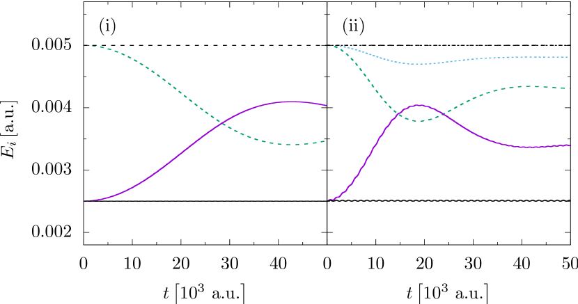
Figure 1: Energies of individual sites. From left to right: 2D (i) and 3D results (ii). Solid lines: energy of the low-frequency oscillator (violet: LSC-IVR, black: FFT), dashed lines: energies of the high-frequency oscillators (turqoise and light blue: LSC-IVR, black: FFT).

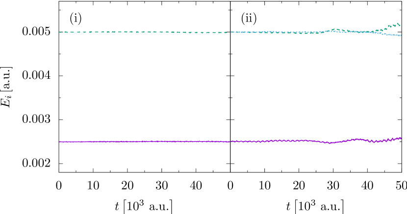
Figure 2: Energies of individual sites, calculated with HK. From left to right: 2D (i), 3D (ii). Solid violet line: energy of the low-frequency oscillator, all dashed lines: energies of the high-frequency oscillators.

All in all, the simple model investigation presented above reveals that the HK propagator, despite relying on classical trajectories, is free from the ZPE leakage. This is a consequence of its elaborate structure which interconnects the trajectories in a highly non-trivial way. Although the considered systems are very simple, the demonstrated absence of the ZPE leakage cannot be a consequence of this simplicity. In contrast, this result should hold for arbitrary systems and thus the goal is to find a proper approximation to the method that preserves the advantages of the HK propagator and circumvents the numerical weaknesses it is suffering from.

V Acknowledgements

Michele Ceotto and Max Buchholz acknowledge financial support from the European Research Council (ERC) under the European Union’s Horizon 2020 research and innovation programme (Grant Agreement No. [647107] – SEMICOMPLEX – ERC-2014-CoG). M.C. acknowledges also the CINECA for the availability of high performance computing resources.

References

- Marx and Hutter (2009) D. Marx and J. Hutter, Ab initio molecular dynamics: basic theory and advanced methods (Cambridge University Press, Cambridge, 2009).
- Tuckerman (2010) M. E. Tuckerman, Statistical mechanics: theory and molecular simulation (Oxford University Press, Oxford, 2010).
- Gao and Truhlar (2002) J. Gao and D. G. Truhlar, Annu. Rev. Phys. Chem. 53, 467 (2002).
- Olsson, Siegbahn, and Warshel (2004) M. H. M. Olsson, P. E. M. Siegbahn, and A. Warshel, J. Am. Chem. Soc. 126, 2820 (2004).
- Habershon, Markland, and Manolopoulos (2009) S. Habershon, T. E. Markland, and D. E. Manolopoulos, J. Chem. Phys. 131, 024501 (2009).
- Ivanov et al. (2010) S. D. Ivanov, O. Asvany, A. Witt, E. Hugo, G. Mathias, B. Redlich, D. Marx, and S. Schlemmer, Nat. Chem. 2, 298 (2010).
- Witt, Ivanov, and Marx (2013) A. Witt, S. D. Ivanov, and D. Marx, Phys. Rev. Lett. 110, 083003 (2013).
- Truhlar (1979) D. G. Truhlar, The Journal of Physical Chemistry 83, 188 (1979).
- Schatz (1983) G. C. Schatz, J. Chem. Phys. 79, 5386 (1983).
- Bowman, Gazdy, and Sun (1989) J. M. Bowman, B. Gazdy, and Q. Sun, J. Chem. Phys. 91, 2859 (1989).
- Miller, Hase, and Darling (1989) W. H. Miller, W. L. Hase, and C. L. Darling, J. Chem. Phys. 91, 2863 (1989).
- hong Lu and Hase (1988) D. hong Lu and W. L. Hase, J. Chem. Phys. 89, 6723 (1988).
- Peslherbe and Hase (1994) G. H. Peslherbe and W. L. Hase, J. Chem. Phys. 100, 1179 (1994).
- Lim and McCormack (1995) K. F. Lim and D. A. McCormack, J. Chem. Phys. 102, 1705 (1995).
- Nyman and Davidsson (1990) G. Nyman and J. Davidsson, J. Chem. Phys. 92, 2415 (1990).
- Varandas and Marques (1992) A. J. C. Varandas and J. M. C. Marques, J. Chem. Phys. 97, 4050 (1992).
- Xie and Bowman (2006) Z. Xie and J. M. Bowman, J. Phys. Chem. A 110, 5446 (2006).
- Schlier (1995) C. Schlier, J. Chem. Phys. 103, 1989 (1995).
- McCormack and Lim (1995) D. A. McCormack and K. F. Lim, J. Chem. Phys. 103, 1991 (1995).
- Sewell et al. (1992) T. D. Sewell, D. L. Thompson, J. Gezelter, and W. H. Miller, Chem. Phys. Lett. 193, 512 (1992).
- Guo, Thompson, and Sewell (1996) Y. Guo, D. L. Thompson, and T. D. Sewell, J. Chem. Phys. 104, 576 (1996).
- Ceriotti, Bussi, and Parrinello (2009) M. Ceriotti, G. Bussi, and M. Parrinello, Phys. Rev. Lett. 103, 030603 (2009).
- Dammak et al. (2009) H. Dammak, Y. Chalopin, M. Laroche, M. Hayoun, and J.-J. Greffet, Phys. Rev. Lett. 103, 1 (2009).
- Brieuc et al. (2016) F. Brieuc, Y. Bronstein, H. Dammak, P. Depondt, F. Finocchi, and M. Hayoun, J. Chem. Theory Comput. 12, 5688 (2016).
- Feynman and Hibbs (1965) R. P. Feynman and A. R. Hibbs, Quantum Mechanics and Path Integrals (McGraw-Hill, New-York, 1965).
- Chandler and Wolynes (1981) D. Chandler and P. Wolynes, J. Chem. Phys. 74, 4078 (1981).
- Craig and Manolopoulos (2004) I. R. Craig and D. E. Manolopoulos, J. Chem. Phys. 121, 3368 (2004).
- Habershon et al. (2013) S. Habershon, D. E. Manolopoulos, T. E. Markland, and T. F. Miller III, Annual review of physical chemistry 64, 387 (2013).
- Ceriotti et al. (2016) M. Ceriotti, W. Fang, P. G. Kusalik, R. H. McKenzie, A. Michaelides, M. A. Morales, and T. E. Markland, Chem. Rev. 116, 7529 (2016).
- Witt et al. (2009) A. Witt, S. D. Ivanov, M. Shiga, H. Forbert, and D. Marx, J. Chem. Phys. 130, 194510 (2009).
- Habershon, Fanourgakis, and Manolopoulos (2008) S. Habershon, G. S. Fanourgakis, and D. E. Manolopoulos, J. Chem. Phys. 129, 074501 (2008).
- Rossi, Ceriotti, and Manolopoulos (2014) M. Rossi, M. Ceriotti, and D. E. Manolopoulos, J. Chem. Phys. 140, 234116 (2014).
- Van Vleck (1928) J. H. Van Vleck, Proc. Natl. Acad. Sci. 14, 178 (1928).
- Littlejohn (1992) R. G. Littlejohn, J. Stat. Phys. 68, 7 (1992).
- Miller (1974) W. H. Miller, Adv. Chem. Phys. 25, 69 (1974).
- Miller (2001) W. H. Miller, J. Phys. Chem. A 105, 2942 (2001).
- Thoss and Wang (2004) M. Thoss and H. Wang, Annu. Rev. Phys. Chem. 55, 299 (2004).
- Kay (2005) K. G. Kay, Annu. Rev. Phys. Chem. 56, 255 (2005).
- Herman and Kluk (1984) M. F. Herman and E. Kluk, Chem. Phys. 91, 27 (1984).
- Kluk, Herman, and Davis (1986) E. Kluk, M. F. Herman, and H. L. Davis, J. Chem. Phys. 84, 326 (1986).
- Kay (1994) K. G. Kay, J. Chem. Phys. 100, 4377 (1994).
- Grossmann (2013) F. Grossmann, Theoretical Femtosecond Physics, 2nd ed., Graduate Texts in Physics (Springer International Publishing, Heidelberg, 2013).
- Heller (1981) E. J. Heller, J. Chem. Phys. 75, 2923 (1981).
- Wehrle, Šulc, and Vaníček (2014) M. Wehrle, M. Šulc, and J. Vaníček, J. Chem. Phys. 140, 244114 (2014).
- de Almeida (1998) A. M. de Almeida, Phys. Rep. 295, 265 (1998).
- Dittrich, Viviescas, and Sandoval (2006) T. Dittrich, C. Viviescas, and L. Sandoval, Phys. Rev. Lett. 96, 1 (2006).
- Dittrich, Gómez, and Pachón (2010) T. Dittrich, E. A. Gómez, and L. A. Pachón, J. Chem. Phys. 132, 214102 (2010).
- de Almeida, Vallejos, and Zambrano (2013) A. M. O. de Almeida, R. O. Vallejos, and E. Zambrano, J. Phys. A Math. Theor. 46, 135304 (2013).
- ichi Koda (2015) S. ichi Koda, J. Chem. Phys. 143, 244110 (2015).
- Bondar et al. (2013) D. I. Bondar, R. Cabrera, D. V. Zhdanov, and H. A. Rabitz, Phys. Rev. A 88, 1 (2013), arXiv:1202.3628 .
- Gottwald and Ivanov (2018) F. Gottwald and S. D. Ivanov, Chem. Phys. 503, 77 (2018).
- Makri and Miller (1987) N. Makri and W. H. Miller, Chem. Phys. Lett. 139, 10 (1987).
- Walton and Manolopoulos (1996) A. R. Walton and D. E. Manolopoulos, Mol. Phys. 87, 961 (1996).
- Herman (1997) M. F. Herman, Chem. Phys. Lett. 275, 445 (1997).
- Elran and Kay (1999a) Y. Elran and K. G. Kay, J. Chem. Phys. 110, 3653 (1999a).
- Elran and Kay (1999b) Y. Elran and K. G. Kay, J. Chem. Phys. 110, 8912 (1999b).
- Kaledin and Miller (2003) A. L. Kaledin and W. H. Miller, J. Chem. Phys. 118, 7174 (2003).
- Ceotto et al. (2009) M. Ceotto, S. Atahan, G. F. Tantardini, and A. Aspuru-Guzik, J. Chem. Phys. 130, 234113 (2009), arXiv:0712.0424 .
- Gabas, Conte, and Ceotto (2017) F. Gabas, R. Conte, and M. Ceotto, J. Chem. Theory Comput. 13, 2378 (2017).
- Ceotto, Di Liberto, and Conte (2017) M. Ceotto, G. Di Liberto, and R. Conte, Phys. Rev. Lett. 119, 010401 (2017).
- Liberto, Conte, and Ceotto (2018) G. D. Liberto, R. Conte, and M. Ceotto, J. Chem. Phys. 148, 014307 (2018).
- Sun and Miller (1999) X. Sun and W. H. Miller, J. Chem. Phys. 110, 6635 (1999).
- Makri and Thompson (1998) N. Makri and K. Thompson, Chem. Phys. Lett. 291, 101 (1998).
- Kühn and Makri (1999) O. Kühn and N. Makri, J. Phys. Chem. A 103, 9487 (1999).
- Batista et al. (1999) V. Batista, M. Zanni, B. Greenblatt, D. Neumark, and W. Miller, J. Chem. Phys. 110, 3736 (1999).
- Skinner and Miller (1999) D. E. Skinner and W. H. Miller, Chem. Phys. 111, 10787 (1999).
- Guallar, Batista, and Miller (2000) V. Guallar, V. S. Batista, and W. H. Miller, J. Chem. Phys. 113, 9510 (2000).
- Wang, Thoss, and Miller (2000) H. Wang, M. Thoss, and W. H. Miller, J. Chem. Phys. 112, 47 (2000).
- Ovchinnikov, Apkarian, and Voth (2001) M. Ovchinnikov, V. A. Apkarian, and G. A. Voth, J. Chem. Phys. 114, 7130 (2001).
- Nakayama and Makri (2003) A. Nakayama and N. Makri, J. Chem. Phys. 119, 8592 (2003).
- Nakayama and Makri (2004) A. Nakayama and N. Makri, Chem. Phys. 304, 147 (2004).
- Tao and Miller (2009) G. Tao and W. H. Miller, J. Chem. Phys. 131 (2009).
- Herman (2014) M. F. Herman, J. Phys. Chem. B 118, 8026 (2014).
- Alemi and Loring (2015) M. Alemi and R. F. Loring, J. Phys. Chem. B 119, 8950 (2015).
- Tao and Miller (2011) G. Tao and W. H. Miller, J. Chem. Phys. 135, 024104 (2011).
- Grossmann (2006) F. Grossmann, J. Chem. Phys. 125, 014111 (2006).
- Buchholz, Grossmann, and Ceotto (2016) M. Buchholz, F. Grossmann, and M. Ceotto, J. Chem. Phys. 144, 094102 (2016).
- Buchholz, Grossmann, and Ceotto (2017) M. Buchholz, F. Grossmann, and M. Ceotto, J. Chem. Phys. 147, 164110 (2017).
- Buchholz, Grossmann, and Ceotto (2018) M. Buchholz, F. Grossmann, and M. Ceotto, J. Chem. Phys. 148, 114107 (2018).
- Koch et al. (2008) W. Koch, F. Großmann, J. Stockburger, and J. Ankerhold, Phys. Rev. Lett. 100, 230402 (2008).
- Koch et al. (2010) W. Koch, F. Großmann, J. T. Stockburger, and J. Ankerhold, Chem. Phys. 370, 34 (2010).
- Heller (1976) E. J. Heller, J. Chem. Phys. 65, 1289 (1976).
- Wang, Sun, and Miller (1998) H. Wang, X. Sun, and W. H. Miller, J. Chem. Phys. 108, 9726 (1998).
- Liu (2015) J. Liu, International Journal of Quantum Chemistry 115, 657 (2015).
- Grossmann (1999) F. Grossmann, Comm. At. Mol. Phys. 34, 141 (1999).
- Lasser and Sattlegger (2017) C. Lasser and D. Sattlegger, Numer. Math. 137, 119 (2017).
- Herman and Coker (1999) M. F. Herman and D. F. Coker, J. Chem. Phys. 111, 1801 (1999).
- Schmidt and Lorenz (2017) B. Schmidt and U. Lorenz, Computer Physics Communications 213, 223 (2017).
- Schmidt and Hartmann (2018) B. Schmidt and C. Hartmann, Computer Physics Communications , (2018).
- Zagoya, Schulman, and Grossmann (2014) C. Zagoya, L. S. Schulman, and F. Grossmann, Journal of Physics A: Mathematical and Theoretical 47, 165102 (2014).