Symanzik Improvement with Dynamical Charm:
A 3+1 Scheme for Wilson Quarks

Abstract

We discuss the problem of lattice artefacts in QCD simulations enhanced by the introduction of dynamical charmed quarks. In particular, we advocate the use of a massive renormalization scheme with a close to realistic charm mass. To maintain O($a$) improvement for Wilson type fermions in this case we define a finite size scheme and carry out a nonperturbative estimation of the clover coefficient $c_{\rm sw}^{\vphantom{()}}$. It is summarized in a fit formula $c_{\rm sw}^{\vphantom{()}}(g_{0}^{2})$ that defines an improved action suitable for future dynamical charm simulations.

1 Introduction

Physicists have been rather fortunate that perturbation theory in the form of low order Feynman diagrams has been largely sufficient to practically establish today’s highly successful Standard Model of elementary particles from experiment. Due to asymptotic freedom even the strongly interacting sector of confined quarks and gluons (QCD) could be pinned down in this way, based on high energy scattering of weakly interacting probes (e.g. $e^{+}\,e^{-}$ and $e^{-}p$). The thus completely characterized theory is expected to also produce the hadronic bound states observed in nature. To extract these predictions—and thus ultimately validate the complete theory—nonperturbative techniques become indispensable.

The only known nonperturbative definition of QCD is the regularization on a lattice which in particular provides a systematic way to extract nonperturbative information about hadrons from the theory by Monte Carlo simulations of QCD on sequences of finite computational lattices. This inflicts however several unavoidable distortions of the theory which need to be controlled. The lattice spacing $a$ acts as an ultraviolet regulator that has to be extrapolated to zero up to tolerable errors. A finite system length $L$ is introduced and has to be made effectively infinite in a similar sense. Finally—as in experiment—all predictions come with statistical errors that have to be small enough for significant comparisons. In particular the symmetries of QCD get modified by the lattice regularization and some of them only re-emerge in the continuum limit $a\to 0$. Very obviously this holds true for infinitesimal translation invariance. Wilson [1] showed that gauge invariance can be preserved on the lattice. It is deemed to be so essential for physics that only such formulations are considered. For the gluons this is achieved by writing the action in terms of parallel transporters around plaquettes or other small closed loops as we shall detail below.

For the quark degrees of freedom more subtle questions arise. The naive gauge covariant discretization of the first derivative in the Dirac action leads to fermion doubling, i.e., an unwanted proliferation of the degrees of freedom. It has turned out that this is in fact related to a certain principal incompatibility between the lattice discretization and chiral invariance [2], which is a very important approximate symmetry in QCD. There are several possibilities to coexist with the corresponding no-go theorem [2]. The present article refers to the choice proposed also by Wilson [3] which nowadays is called Wilson fermions. By adding the so-called Wilson term to the action (see below) the one-to-one correspondence between lattice Dirac fields and physical quarks is restored and the vectorial flavor symmetries are intact even in the presence of the lattice. There is however a price to pay for this bonus. The Wilson term violates chiral symmetry, which must emerge non-trivially in the continuum limit. Moreover, without further precautions, the lattice cutoff effects vanish only asymptotically linearly in $a$. The gluon action alone, and also certain other fermion discretizations, lead to a behavior proportional to $a^{2}$ which much facilitates the extrapolation and enhances the precision in and the reliability of this step. A further complication due to the missing chiral invariance at finite $a$ is the need to control an additive quark mass renormalization. We only briefly mention here that technically the dynamical quarks dominate the simulation costs. The degree to which this is the case depends on the chosen discretization with Wilson fermions being one of the cheaper options.

To limit the simulation costs, lattice calculations have proceeded through a series of approximations concerning the quantum effects due to virtual dynamical flavor contributions. At first they were neglected altogether in the quenched approximation. Then, to have a unitary theory and to capture the most important loop effects, two or three light flavors were included. In this article we are concerned with the next level where we add the dynamical charmed quark. It has a much larger mass $m_{{\rm c}}$ compared to up, down or strange quarks, and this can lead to cutoff effects proportional to the dangerously large dimensionless factor $am_{{\rm c}}$. Special measures toward their control are in the focus of this article. In particular we suggest and formulate Symanzik improvement of the Wilson theory in a massive renormalization scheme. The Sheikholeslami-Wohlert coefficient [4] is determined non-perturbatively with a massive charm quark.

Massive renormalization schemes are not new in the context of a reduction of ${\rm O}(\!(am_{\rm c})^{n}\!)$ effects. They have been used (sometimes implicitly) for space-time symmetric formulations [5, 6, 7, 8, 9] and with broken space-time symmetry [10, 11, 12, 13, 14, 15, 16, 17, 18, 19, 20]. The latter arise from considerations of effective field theories for heavy quarks and have so far been applied to quenched quarks or heavy quarks treated in a mixed action approach. References [10, 11, 12, 13, 14, 15, 16, 17, 18, 19, 20] aim at a reduction of the quadratic and higher, $n\geq 2$, terms by tree-level and one-loop perturbation theory. We here focus just on the non-perturbative removal of the linear term in $am_{\rm c}$.

This paper is a highly condensed summary of the PhD thesis [21] by Felix Stollenwerk. In sect. 2 we review on-shell Symanzik O($a$) improvement followed by the comparisons of mass dependent and independent renormalization schemes in sect. 3. In sect. 4 we define a line of constant physics by maintaining a set of finite size observables as $a$ is changed. In sect. 5 this is employed for a nonperturbative determination of the improvement coefficient $c_{\rm sw}^{\vphantom{()}}$ in a scheme of three light flavors together with the close to physical dynamical charm quark. A fit formula is presented that allows to implement this action in future large volume simulations at and close to the physical point. We end with some conclusions in sect. 6.

2 Symanzik improvement

Symanzik has put forward a method [22, 23, 24] to accelerate the continuum limit in lattice field theories by increasing the power of $a$ characterizing the leading lattice artifacts. It is routinely applied to Wilson fermions to achieve an $a^{2}$ continuum scaling. This so-called Symanzik improvement programme starts from an effective continuum theory which first only describes a given lattice theory including its leading order artefacts. In a renormalizable quantum field theory we are at first instructed to include in the action a combination of all possible terms up to (including) mass dimension four which possess the desired symmetry. They typically are small in number and are related to the number of free (renormalized) parameters. To reproduce the leading cutoff effects of O($a$), the scope has to be widened to all such operators of dimension five. They appear multiplied by dimensionless coefficient functions times an explicit factor of $a$. They could be determined by imposing a sufficient number of conditions where observables of the lattice theory are matched. These are analogous to renormalization conditions to fix the relevant terms up to dimension four. In a next step one then modifies the lattice action such that the dimension five terms in the associated effective continuum theory become zero. This can be achieved by including in the lattice theory a linear combination of discretized versions of the dimension five operators with suitably tuned coefficients. Any ambiguity in this step only affects the uncancelled higher order artefacts. What is exploited here is the structure of the effective theory which allows to describe all O($a$) artefacts by a finite set of parameters by organizing all possible terms according to their naive dimension. This could in principle be invalidated by large anomalous dimensions due to quantum corrections. For asymptotically free theories like QCD this does however not happen to any finite order of perturbation theory. In this sense the Symanzik programme is expected to work in a similar way as renormalizability and thus the existence of the continuum limit.

In the following we shall restrict our focus on the simpler on-shell Symanzik improvement [25, 26]. This means that we only improve observables that are derived from correlation functions with operators separated by physical distances that remain finite in the continuum limit. Then the use of the quantum equations of motion is justified which allows to relate dimension five operators to each other and thus to reduce the number of independent terms that have to be managed. As we shall report below we then need, apart from terms related to quark masses, only one single term, the Pauli or, on the lattice, the clover-leaf term [4] to cancel O($a$) artefacts in QCD.

We now summarize the structure of the Symanzik effective (continuum) Lagrangian that describes lattice QCD with $N_{\rm f}$ flavors of Wilson quarks with a diagonal mass matrix $M$, including O($a$) lattice artefacts,

$$\mathcal{L}_{\mathrm{Sym}} =-\tfrac{1}{2g_{0}^{2}}\,\mathrm{tr}[F_{\mu\nu}F_{\mu\nu}]+\bar{\psi}\not{D}\psi+\bar{\psi}M\psi+\rho\,\mathrm{tr}[M]\,\bar{\psi}\psi$$

$$\quad+a\sigma_{0}\,\bar{\psi}\sigma_{\mu\nu}F_{\mu\nu}\psi+a\sigma_{1}\,\bar{\psi}M^{2}\psi+a\sigma_{2}\,\mathrm{tr}[M]\,\bar{\psi}M\psi+a\sigma_{3}\,\mathrm{tr}{[M^{2}]}\,\bar{\psi}\psi$$

$$\quad+a\sigma_{4}\,(\mathrm{tr}[M])^{2}\,\bar{\psi}\psi+a\sigma_{5}\,\mathrm{tr}[M]\,\mathrm{tr}[F_{\mu\nu}F_{\mu\nu}]\,.$$ (2.1)

The first line contains the dimension four terms. The anti-Hermitian algebra valued field strength is denoted as usual by $F_{\mu\nu}$ and $\not{D}$ is the covariant Dirac operator. A subtlety here is, that due to the missing chiral symmetry of the lattice action, the adjustable constant $\rho$ is required to match the renormalization pattern of the lattice theory which differs for the flavor singlet and non-singlet components in $M$. The remaining lines show the dimension five operators. We have already implemented simplifications from using the equations of motion (on-shell improvement) here. In this way we could drop the terms $a\bar{\psi}D^{2}\psi$, $a\bar{\psi}\not{D}M\psi$ and $a\mathrm{tr}[M]\bar{\psi}\not{D}\psi$.

Similarly to the action also currents appearing in correlation functions have to be nontrivially matched by the Symanzik effective theory. One has to allow for the mixing of terms of the same and the next higher dimension as far as they share all symmetries preserved by the lattice theory. We here restrict ourselves to the off-diagonal axial vector and pseudoscalar currents made of quarks of flavor $i\not=j$,

$$A_{\mu}^{ij} =\bar{\psi}_{i}\gamma_{\mu}\gamma_{5}\psi_{j}\,,\quad P^{ij}=\bar{\psi}_{i}\gamma_{5}\psi_{j}\,.$$ (2.2)

Their mixing pattern is

$$(A_{\mathrm{Sym}})_{\mu}^{ij} =\left\{1+\omega_{1}\,a\mathrm{tr}[M]+\omega_{2}\,a(m_{i}+m_{j})\right\}A_{\mu}^{ij}+\omega_{0}\,a\partial_{\mu}P^{ij}\,,$$ (2.3)

and

$$(P_{\mathrm{Sym}})^{ij} =\left\{1+\omega_{1}^{\prime}\,a\mathrm{tr}[M]+\omega_{2}^{\prime}\,a(m_{i}+m_{j})\right\}P^{ij}\,.$$ (2.4)

In continuum QCD chiral symmetry implies the PCAC relation for the renormalized currents. Formally, i.e., disregarding renormalization for the moment, it reads

$$\partial_{\mu}A_{\mu}^{ij}=(m_{i}+m_{j})P^{ij}$$ (2.5)

and it holds as an operator relation. This means that the above identity may be inserted in correlators with suitable operators $O$

$$\langle\partial_{\mu}A_{\mu}^{ij}O\rangle=(m_{i}+m_{j})\langle P^{ij}O\rangle\,.$$ (2.6)

Such relations are typically violated by O($a$) artefacts in the lattice theory. They thus may serve as a source of relations which allow to determine coefficients of O($a$) corrections in the Symanzik effective theory and ultimately in the improved lattice theory.

3 Mass (in)dependent renormalization scheme and improvement

In mass independent renormalization schemes for QCD the conditions that define the renormalized theory are formulated at vanishing quark masses in terms of an external renormalization scale $\mu$ only. This in particular leads to relatively simple renormalization group equations with $\beta$- and $\gamma$-functions depending on the dimensionless coupling only. In the technically convenient finite size schemes the system size $L$ is often used as external scale. In this article we shall argue that in the presence of dynamical charmed quarks, mass dependent schemes, where renormalization factors are allowed to depend on quark masses, offer practical advantages.

3.1 Mass independent case

In the case of mass independent renormalization schemes the relation between bare and renormalized gauge coupling reads (without improvement)

$$g_{\mathrm{\scriptscriptstyle R}}^{2}=Z_{g}(g_{0}^{2},a\mu)g_{0}^{2},$$ (3.7)

and $Z_{g}$ is determined in this way, once a suitable $g_{\mathrm{\scriptscriptstyle R}}$ has been defined. The relation between bare and renormalized masses has the structure

$$m_{\mathrm{\scriptscriptstyle R},i}=Z_{m}(g_{0}^{2},a\mu)\left[m_{\mathrm{q,}i}+(r_{m}(g_{0}^{2})-1)\,\mathrm{tr}[M_{\rm q}]/N_{\rm f}\right]$$ (3.8)

involving the bare subtracted quark masses of flavor $i$

$$m_{\mathrm{q,}i}=m_{i}-m_{\mathrm{crit}}(g_{0}^{2})\,,\quad M_{\rm q}={\rm diag}(m_{\rm q,1},\ldots,m_{\rm q,N_{\rm f}})\,.$$ (3.9)

We remind here that both the necessity of the nonzero critical bare mass $m_{\rm crit}$ and the extra renormalization constant $r_{m}$ refer to our lattice regulator which breaks chiral symmetry.

To implement Symanzik O($a$) improvement the above relations have to be augmented by additional terms that are proportional to an explicit factor $a$ [25]. In the case of the coupling this is of a relatively simple form. All we have to do is to replace $g_{0}^{2}$ in (3.7) and (3.8) by

$$\tilde{g}_{0}^{2}=g_{0}^{2}\left(1+ab_{\rm g}(g_{0}^{2})\,\mathrm{tr}[M_{\rm q}]/N_{\rm f}\right)\,,$$ (3.10)

and to add to our lattice action the ‘clover’ contribution, first introduced by Sheikholeslami and Wohlert (SW) [4],

$$S_{\scriptscriptstyle\rm SW}=a^{5}c_{\rm sw}^{\vphantom{()}}(g_{0}^{2})\sum_{x}\bar{\psi}(x)\frac{i}{4}\sigma_{\mu\nu}\hat{F}_{\mu\nu}(x)\psi(x)\,,$$ (3.11)

with $\hat{F}_{\mu\nu}(x)$ being a lattice discretization of the (anti-Hermitian) field strength tensor at site $x$. More details on the lattice action follow in the next section. This extra term corresponds to the contribution proportional to $\sigma_{0}$ in (2.1), while the $b_{\rm g}$ modification in (3.10) represents the $\sigma_{5}$ part on the lattice.

Sandwiching the matrix $M+a\{\sigma_{1}M^{2}+\sigma_{2}\mathrm{tr}[M]M+\sigma_{3}\mathrm{tr}[M^{2}]+\sigma_{4}(\mathrm{tr}[M])^{2}\}$ between $\bar{\psi}$ and $\psi$ summarizes the remaining terms in (2.1). Following the notation of [27] the corresponding terms are included in the lattice theory by using an improved renormalized mass of flavor $i$

$$m_{\mathrm{\scriptscriptstyle R},i} =Z_{m}(\tilde{g}_{0}^{2},a\mu)\bigg{[}m_{\mathrm{q,}i}+\left(r_{m}(\tilde{g}_{0}^{2})-1\right)\frac{\mathrm{tr}[M_{\rm q}]}{N_{\rm f}}+a\bigg{\{}b_{m}(g_{0}^{2})m_{\mathrm{q,}i}^{2}+\bar{b}_{m}(g_{0}^{2})\mathrm{tr}[M_{\rm q}]\,m_{\mathrm{q,}i}$$

$$\qquad\qquad\qquad\qquad\qquad+\left(r_{m}(g_{0}^{2})d_{m}(g_{0}^{2})-b_{m}(g_{0}^{2})\right)\frac{\mathrm{tr}[M_{\rm q}^{2}]}{N_{\rm f}}$$

$$\qquad\qquad\qquad\qquad\qquad+\left(r_{m}(g_{0}^{2})\bar{d}_{m}(g_{0}^{2})-\bar{b}_{m}(g_{0}^{2})\right)\frac{\left(\mathrm{tr}[M_{\rm q}]\right)^{2}}{N_{\rm f}}\bigg{\}}\bigg{]}$$ (3.12)

on the lattice. If now physical observables are parameterized by $g_{\mathrm{\scriptscriptstyle R}}$ and $m_{\mathrm{\scriptscriptstyle R},i}$ then we expect them to converge to their continuum limits at a rate proportional to $a^{2}$, provided that the prefactors of all improvement terms have the correct values to cancel all O($a$) terms along with the divergences.

In practice, for $N_{\rm f}\leq 3$, the mass dependent improvement terms have been found to lead to small effects. Thus they could be set to their low order perturbative values without spoiling the targeted precision. Only the $c_{\rm sw}^{\vphantom{()}}$ term (beside operator improvements to be discussed later) was found to be essential. For this reason the ALPHA collaboration and others have engaged in nonperturbative computations of $c_{\rm sw}^{\vphantom{()}}(g_{0}^{2})$ for various numbers of light flavors $0\leq N_{\rm f}\leq 4$. They are found in refs. [28, 29, 30, 31, 32, 33, 34].

If we want to treat the physical charm quark in a mass independent scheme as discussed above, then there appear improvement terms multiplied by the charm mass $am_{\mathrm{q,}{\rm c}}$. Also $\mathrm{tr}[M_{\rm q}]$ will now be dominated by charm. A rough estimate puts these terms to around 0.5 and about an order of magnitude larger than the analogous strange contributions for lattice spacings on the order of $0.1\,{\rm fm}$. Thus the respective $b_{*}$ and other coefficients must be known much more precisely than for the light flavors. This is even true for the virtual contributions in the absence of valence charm quarks. Even at the level $a^{0}$ the term $r_{m}-1$ is enhanced and very high precision for $r_{m}$ may be required. A simultaneous nonperturbative determination of all these improvement coefficients seems impractical and we hence rather give up the technical convenience of mass independent schemes and switch to massive ones.

3.2 Mass dependent case

In massive renormalization schemes the $Z$ factors are allowed to depend on the mass matrix $M$. We take

$$g_{\mathrm{\scriptscriptstyle R}}^{2}=\tilde{Z}_{g}(g_{0}^{2},a\mu,aM)g_{0}^{2}\,,$$ (3.13)

and

$$m_{\mathrm{\scriptscriptstyle R},i}=\tilde{Z}_{m}^{i}(g_{0}^{2},a\mu,aM)\left[m_{i}-\tilde{m}_{\rm crit}(g_{0}^{2},a\mathrm{tr}[M_{\rm q}])\right]\,.$$ (3.14)

Clearly all the correction terms proportional to $am_{\mathrm{q,}i}$ in (3.10) and (3.12) can now be absorbed into the multiplicative $\tilde{Z}$ factors. The term proportional to $(r_{m}-1)$ in (3.12) can be reproduced by the $a\mathrm{tr}[M_{\rm q}]$ dependent critical mass $\tilde{m}_{\mathrm{crit}}$. It remains to keep the clover term (3.11) with a mass dependent coefficient function $\tilde{c}_{\rm sw}(g_{0}^{2},aM)$. Note that the mass dependent O($a$) modification of this improvement term formally only contributes at O($a^{2}$) and in this sense could be dropped. But in passing to mass dependent renormalization we want to avoid these O($a^{2}$) effects which are enhanced by the charm mass and keep the mass dependence of $\tilde{c}_{\rm sw}$, too.

Beside the definition of renormalized parameters and the SW term the scheme has to include improved operators, and we focus on $A_{\mu}^{ij}$ and $P^{ij}$ as before. The definitions (2.2) and (2.4) are now reinterpreted in terms of lattice fields all at the same site. By similar considerations as for the action we set

$$(A_{\scriptscriptstyle\rm R})^{ij}_{\mu}=\tilde{Z}_{\scriptscriptstyle\rm A}^{ij}(g_{0}^{2},aM)\left[A^{ij}_{\mu}+a\tilde{c}_{\scriptscriptstyle\rm A}(g_{0}^{2},aM)\partial_{\mu}P^{ij}\right]$$ (3.15)

and

$$(P_{\scriptscriptstyle\rm R})^{ij}=\tilde{Z}_{\scriptscriptstyle\rm P}^{ij}(g_{0}^{2},a\mu,aM)P^{ij}$$ (3.16)

for the renormalized and improved currents in our massive scheme.For the inclusion of an $M$ dependence in $\tilde{c}_{\scriptscriptstyle\rm A}$ we refer to the earlier discussion for $\tilde{c}_{\rm sw}$.

3.3 A 3+1 flavor scheme

So far we have assumed no degeneracies in our arbitrary quark mass matrix. For our later numerical work we shall find it advantageous to reduce the number of relevant mass parameters by approximating nature by a simplified pattern. We shall be guided in principle by keeping the charm mass and the value of $\mathrm{tr}[M_{\rm q}]$ close to their physical values. At the same time we deal with only two independent masses by setting

$$M_{\rm q}={\rm diag}(m_{\mathrm{q,}l},m_{\mathrm{q,}l},m_{\mathrm{q,}l},m_{\mathrm{q,}{\rm c}})\,.$$ (3.17)

Beside the (subtracted) charm mass $m_{\mathrm{q,}{\rm c}}$ we have introduced a light quark mass $m_{\mathrm{q,}l}$ which is imagined to equal approximately a third of the strange mass. We expect this scheme to be at the same time numerically manageable and close enough to the eventual target physics to avoid large mass dependent artefacts and renormalization effects.

In the following we shall be concerned with this kind of massive renormalization scheme and will omit again the tildes over the improvement coefficients $c_{\scriptscriptstyle\rm A},c_{\rm sw}^{\vphantom{()}}$. Moreover we shall in particular embark on a nonperturbative calculation of $c_{\rm sw}^{\vphantom{()}}(g_{0}^{2},aM_{\rm q})$ with $M_{\rm q}$ chosen as in eq. (3.17).

4 Scaling at constant finite volume physics

To prepare for a nonperturbative determination of $c_{\rm sw}^{\vphantom{()}}$ we now envisage the construction of a set of lattice configurations with bare parameters that correspond to a line of constant physics (LCP) with fixed renormalized parameters in a finite volume scheme and a well defined discretization. This is done for a number of lattice spacings $a$ and $c_{\rm sw}^{\vphantom{()}}$ values in the relevant range. The quark masses for $N_{\rm f}=3+1$ are tuned to the vicinity of the values described at the end of the last section. In the next section we consider scaling violations in the PCAC relation (2.5) to single out ‘optimal’ $c_{\rm sw}^{\vphantom{()}}$ values for each of our lattice spacings which can then be represented and interpolated by a smooth fit formula.

We implement Schrödinger functional (SF) boundary conditions [35, 36] to set up our finite volume scheme. The 3+1 flavors of Wilson quarks are coupled to gluons weighted with the tree level improved Lüscher–Weisz gauge action [26]. Instead of compiling all details of these definitions we refer here to [34] where almost the same setup has been used. The only small difference is that for the fermionic boundary improvement coefficient $\tilde{c}_{\rm t}$, that is called $c_{\mathrm{\scriptscriptstyle F}}$ in [34], we use the tree level approximation $\tilde{c}_{\rm t}=1$. We choose equal temporal and spatial extents $T=L$. The boundary gauge fields $C_{k},C_{k}^{\prime}$ will first be set to zero in this section and to the nontrivial values given in [34, 28] in the following section. Our fermion fields are periodic in the space direction, i.e., the freedom to insert a periodicity angle $\theta$ into the SF is not used here. The bare quark masses will be specified in terms of the well known hopping parameters

$$\kappa_{l} =\frac{1}{2(am_{l}+4)}\,, \kappa_{\rm c} =\frac{1}{2(am_{{\rm c}}+4)}\,.$$ (4.18)

4.1 Finite size definition of the LCP

We start with the definition of a renormalized coupling that we denote by $\Phi_{1}$. In recent years it has turned out that coupling constants derived from the gradient flow [37, 38] have an excellent signal quality for finite tori [39, 40] and for SF boundary conditions [41] at the range of system sizes that we shall want to simulate. We employ the coupling given by the expectation value of the action density

$$\Phi_{1}=\frac{t^{2}}{\mathcal{N}}\sum_{\mu\nu}\left\langle-\tfrac{1}{2}\mathrm{tr}[G_{\mu\nu}^{2}(x,t)]\right\rangle\Big{|}_{\scalebox{0.7}{$x_{0}=T/2,t=c^{2}L^{2}/8$}}\,.$$ (4.19)

In this formula $G_{\mu\nu}$ is the (anti-Hermitian traceless) clover field strength of the ‘flowed’ field and its flow time argument $t$ is tied to the system size by

$$c=0.3\,.$$ (4.20)

The lattice flow equation is based on the simple Wilson plaquette action, i.e., we work with the Wilson flow. The normalization factor ${\cal N}$, which implies $\Phi_{1}=g_{0}^{2}+{\rm O}(g_{0}^{4})$ in perturbation theory, has been derived in [41].

Apart from the coupling that runs with the system size $T=L$ we need two more dimensionless renormalized quantities to fix the light and charm masses. To that end we introduce the SF correlations

$$f_{\rm A}^{ij}{(x_{0})} =-\frac{1}{2}\big{\langle}A_{0}^{ij}{(x_{0})}{\cal O}^{ji}\big{\rangle}\,, f_{\rm P}^{ij}{(x_{0})} =-\frac{1}{2}\big{\langle}P^{ij}{(x_{0})}{\cal O}^{ji}\big{\rangle}\,,$$ (4.21)

with the lattice currents (2.2). The SF boundary operator [25]

$${\cal O}^{ij}=a^{6}\sum_{\vec{x},\vec{y}}\bar{\zeta}^{i}(\vec{x})\gamma_{5}\zeta^{j}(\vec{y})$$ (4.22)

is built from boundary fields at $x_{0}=0$ and yields a nonzero correlation. We next form the improved axial correlation

$$f_{\rm A,I}^{ij}=f_{\rm A}^{ij}+ac_{\scriptscriptstyle\rm A}\tilde{\partial}_{0}f_{\rm P}^{ij}$$ (4.23)

involving the symmetric lattice derivative $\tilde{\partial}_{0}$. An effective meson mass times system size is now coded into

$$\Phi_{2}=-\tilde{\partial}_{0}\log\!\big{(}f_{\rm A,I}^{12}(x_{0})\big{)}\big{|}_{x_{0}=T/2}\times T\,.$$ (4.24)

For very large $T$ we would isolate the mass of the pseudoscalar non-singlet meson of two different light quark species. At finite $T$ we instead have a combination of this mass and higher levels in the same channel with weights given by universal amplitude ratios [42]. In a third quantity we excite states with the quantum number of a singly charmed meson (fourth flavor) and take

$$\Phi_{3}=-\tilde{\partial}_{0}\log\!\big{(}f_{\rm A,I}^{14}(x_{0})\big{)}\big{|}_{\scriptscriptstyle x_{0}=T/2}\times T-\tfrac{1}{2}\Phi_{2}\,.$$ (4.25)

The reason for the subtraction of $\Phi_{2}$ is as follows. We will have to solve the complicated tuning task to find values of $g_{0}^{2},\kappa_{l},\kappa_{\rm c}$ that produce certain soon to be prescribed values of $\Phi_{1,2,3}$. This task is facilitated if $\Phi_{3}$ is sensitive to $\kappa_{\rm c}$ and shows only weak dependence on $\kappa_{l}$. The subtraction cancels the latter dependence in the most naive constituent quark model. In $N_{\rm f}=2$ simulations it has been verified that this property holds in an approximate sense also beyond such a naive scenario.

Another remark is in order to why we use a component of the axial vector rather than the pseudoscalar current to excite the desired quantum numbers. At large $T$ the same meson mass would be isolated with the admixtures at finite $T$ being different in the two cases. The PCAC relation implies that our $\Phi_{2}$ vanishes in the chiral limit, while this would not be the case for the analogous quantity derived with the $P^{12}$ correlator. Hence our choice is expected to optimize the tuning sensitivity for the light mass $\kappa_{l}$. Finally also the inclusion of the improvement term (with perturbative 1-loop $c_{\scriptscriptstyle\rm A}$ [43]) in $f_{\rm A,I}$ is not a necessity here and, again at $N_{\rm f}=2$, it has been seen to make little effect. Nevertheless we keep it as part of our choice.

4.2 Values of $\Phi_{1,2,3}$

Although not practical, a ‘Gedanken simulation’ may be useful to appreciate the well-defined status of our finite volume quantities. We may imagine to simulate QCD on a lattice with negligible cutoff and finite size effects where the bare lattice parameters are tuned such that pion, kaon, D-meson masses and a scale such as the pion decay constant equal their values compiled by the particle data group. From the resulting physical values of the renormalization group invariant (RGI) quark masses, $M_{\rm u},\,M_{\rm d},\,M_{\rm s},\,M_{\rm c}$ we could then easily switch to a flavor SU(3) symmetric point $M_{l}=(M_{\rm u}+M_{\rm d}+M_{\rm s})/3$ for the three light species keeping $M_{\rm c}$. Then $a$ would be known in physical units and we may lower $T/a=L/a$ such that we find $L\approx 0.8\,{\rm fm}$, for example, still having $L/a\gg 1$. On the resulting lattice we read off universal continuum values for $\Phi_{1,2,3}$.

The above strategy is, of course, impractical. Instead we have to somehow deduce the $\Phi_{i}$ with sufficient precision, in order to then on a series of LCP lattices tune $c_{\rm sw}^{\vphantom{()}}$ for O($a$) improvement and to later use this information to reach acceptably small cutoff effects in reasonably large volume simulations. The choice of the system size $L$ together with the feasible $L/a$ determine for which $g_{0}^{2}$ we obtain nonperturbative information on $c_{\rm sw}^{\vphantom{()}}$. It should end up in a range useful for the final simulations.

Our strategy to determine $\Phi_{i}$ is to use here the approximation $N_{\rm f}=2$ with quenched strange and charmed quarks and configurations from earlier simulationsof the ALPHA collaboration [44, 45] together with additional measurements and some newly created configurations as well. For details on these well-defined but tedious estimations we refer to [21]. We here just report the outcome in the form of values

$$\Phi_{1}^{\ast}=7.31,\quad\Phi_{2}^{\ast}=0.59,\quad\Phi_{3}^{\ast}=5.96.$$ (4.26)

These numbers emerge from the $N_{\rm f}=2$ computation with errors at the percent levelbut are now taken to define our LCP which in the continuum limit yields a finite slab of continuum QCD with SF boundary conditions.

An important question is now to which precision we have to tune our $N_{\rm f}=3+1$ lattices to the above target values $\Phi_{i}^{\ast}$ to then determine $c_{\rm sw}^{\vphantom{()}}(g_{0}^{2})$ along the LCP. By a chain of heuristic considerations given in more detail in [21] we arrive at the requirement

$$\frac{\Delta\Phi_{1}}{\Phi_{1}^{\ast}} \lesssim 4\%\,, \frac{\Delta\Phi_{2}}{\Phi_{2}^{\ast}} \lesssim 10\%\,, \frac{\Delta\Phi_{3}}{\Phi_{3}^{\ast}} \lesssim 4\%\,.$$ (4.27)

This corresponds roughly to 5% precision in the scale $T$ and the charm mass and 11% in the light mass. As discussed earlier the closeness to the physical charm mass is of particular relevance to avoid large cutoff effects proportional to the deviation $\Delta m_{\mathrm{q,}{\rm c}}$. The precise values of the light quark masses, which are dominantly controlled by $\Phi_{2}$, on the other hand appear to be less critical.

4.3 Lattice realization of the LCP

We now report on a set of simulation results with lattices tuned to $\Phi_{i}^{\ast}$ within the required precision. They were found from a first set of exploratory simulations in the right range followed by multidimensional interpolations. They serve to predict the ‘right’ values of $g_{0},\kappa_{l},\kappa_{\rm c}$ which are then confirmed or fed into refined interpolations. The final results from this somewhat demanding procedure (see [21] for more details) are collected in table 1. Note that a range of $c_{\rm sw}^{\vphantom{()}}$ is covered for each value $T^{\ast}\!/a$.

After some initial tests, all simulations have been performed in a (2+1+1)-flavor setup, i.e., a degenerate doublet of light quarks is simulated by HMC [46] and the two remaining quark species are incorporated by the RHMC algorithm [47, 48]. In general, the simulations are conducted along the lines of Ref. [49], appendix A, and more details and a cost figure will be provided [50]. Due to the enhanced spectral gap in the Dirac operator with SF boundary conditions and non-vanishing physical quark masses, the performed HMC simulations are very stable and unproblematic.

$c_{\rm sw}^{\vphantom{()}}$	$g_{0}^{2}$	$\kappa_{l}$	$\kappa_{\rm c}$	$\Phi_{1}$	$\Phi_{2}$	$\Phi_{3}$
$T^{\ast}\!/a=8$
$1.9$	$1.7848$	$0.13741$	$0.12033$	$7.17(4)$	$0.59(3)$	$5.95(1)$
$2.0$	$1.8067$	$0.13645$	$0.11960$	$7.17(3)$	$0.56(2)$	$5.99(1)$
$2.1$	$1.8340$	$0.13560$	$0.11900$	$7.36(5)$	$0.61(3)$	$6.02(1)$
$2.2$	$1.8534$	$0.13450$	$0.11820$	$7.17(5)$	$0.60(3)$	$6.03(1)$
$2.3$	$1.8825$	$0.13369$	$0.11770$	$7.36(3)$	$0.62(2)$	$5.97(1)$
$2.4$	$1.9069$	$0.13278$	$0.11750$	$7.31(4)$	$0.57(3)$	$5.93(1)$
$T^{\ast}\!/a=12$
$1.8$	$1.7334$	$0.13742$	$0.12776$	$7.13(5)$	$0.58(3)$	$5.93(2)$
$1.9$	$1.7600$	$0.13656$	$0.12714$	$7.26(4)$	$0.60(3)$	$5.92(2)$
$2.0$	$1.7876$	$0.13573$	$0.12653$	$7.35(5)$	$0.62(3)$	$5.99(3)$
$2.1$	$1.8152$	$0.13486$	$0.12591$	$7.29(6)$	$0.60(4)$	$5.93(3)$
$2.2$	$1.8423$	$0.13401$	$0.12529$	$7.42(7)$	$0.60(4)$	$5.91(3)$
$T^{\ast}\!/a=16$
$1.5$	$1.6266$	$0.13918$	$0.13224$	$7.38(9)$	$0.56(2)$	$5.93(3)$
$1.6$	$1.6482$	$0.13825$	$0.13139$	$7.42(10)$	$0.61(2)$	$6.06(7)$
$1.7$	$1.6741$	$0.13741$	$0.13087$	$7.29(8)$	$0.59(2)$	$5.84(5)$
$1.8$	$1.7036$	$0.13661$	$0.13018$	$7.32(7)$	$0.57(2)$	$5.90(5)$
$1.9$	$1.7331$	$0.13582$	$0.12949$	$7.44(9)$	$0.59(2)$	$5.94(3)$
$2.0$	$1.7626$	$0.13503$	$0.12880$	$7.46(7)$	$0.59(2)$	$6.03(4)$
$T^{\ast}\!/a=20$
$1.5$	$1.5868$	$0.13822$	$0.13287$	$7.20(7)$	$0.61(2)$	$5.91(8)$
$1.6$	$1.6153$	$0.13749$	$0.13240$	$7.30(10)$	$0.57(2)$	$5.91(5)$
$1.7$	$1.6434$	$0.13669$	$0.13178$	$7.29(7)$	$0.60(2)$	$5.85(5)$
$1.8$	$1.6714$	$0.13588$	$0.13126$	$7.49(5)$	$0.63(2)$	$5.81(6)$
$1.9$	$1.6993$	$0.13504$	$0.13046$	$7.36(9)$	$0.62(2)$	$5.81(8)$
$T^{\ast}\!/a=24$
$1.5$	$1.5527$	$0.13751$	$0.13325$	$7.19(6)$	$0.62(2)$	$6.02(8)$
$1.6$	$1.5783$	$0.13672$	$0.13253$	$7.23(11)$	$0.59(1)$	$6.02(6)$
$1.7$	$1.6065$	$0.13595$	$0.13202$	$7.24(9)$	$0.62(2)$	$6.00(5)$
$1.8$	$1.6344$	$0.13515$	$0.13132$	$7.11(7)$	$0.56(1)$	$5.87(6)$

Table 1: Results for tuning to the line of constant physics, eq. (4.26), at various values of $c_{\rm sw}^{\vphantom{()}}$.

5 Determination of $c_{\rm sw}^{\vphantom{()}}$

$c_{\rm sw}^{\vphantom{()}}$	$g_{0}^{2}$	$\kappa_{l}$	$\kappa_{\rm c}$	$T^{*}m^{ud}$	$T^{*}M^{ud}$	$T^{*}\Delta M^{ud}$
$T^{*}\!/a=8$
$1.9$	$1.7848$	$0.13741$	$0.12033$	$0.504(7)$	$0.684(25)$	$+0.047(7)$
$2.0$	$1.8067$	$0.13645$	$0.11960$	$0.491(8)$	$0.621(23)$	$+0.028(7)$
$2.1$	$1.8340$	$0.13560$	$0.11900$	$0.509(8)$	$0.707(32)$	$+0.021(8)$
$2.2$	$1.8534$	$0.13450$	$0.11820$	$0.516(8)$	$0.643(28)$	$-0.014(8)$
$2.3$	$1.8825$	$0.13369$	$0.11770$	$0.521(9)$	$0.724(30)$	$-0.013(8)$
$2.4$	$1.9069$	$0.13278$	$0.11750$	$0.521(10)$	$0.723(31)$	$-0.016(9)$
$T^{*}\!/a=12$
$1.8$	$1.7334$	$0.13742$	$0.12776$	$0.247(4)$	$0.311(11)$	$+0.032(4)$
$1.9$	$1.7600$	$0.13656$	$0.12714$	$0.242(4)$	$0.306(9)$	$+0.012(7)$
$2.0$	$1.7876$	$0.13573$	$0.12653$	$0.237(4)$	$0.300(11)$	$+0.020(5)$
$2.1$	$1.8152$	$0.13486$	$0.12591$	$0.243(5)$	$0.300(10)$	$-0.004(7)$
$2.2$	$1.8423$	$0.13401$	$0.12529$	$0.223(4)$	$0.267(11)$	$-0.011(6)$
$T^{*}\!/a=16$
$1.5$	$1.6266$	$0.13918$	$0.13224$	$0.160(3)$	$0.192(6)$	$+0.026(3)$
$1.6$	$1.6482$	$0.13825$	$0.13139$	$0.159(2)$	$0.164(5)$	$+0.018(4)$
$1.7$	$1.6741$	$0.13741$	$0.13087$	$0.156(2)$	$0.139(6)$	$+0.014(3)$
$1.8$	$1.7036$	$0.13661$	$0.13018$	$0.167(2)$	$0.144(6)$	$+0.004(3)$
$1.9$	$1.7331$	$0.13582$	$0.12949$	$0.165(3)$	$0.136(6)$	$-0.008(3)$
$2.0$	$1.7626$	$0.13503$	$0.12880$	$0.154(2)$	$0.113(6)$	$-0.015(4)$
$T^{*}\!/a=20$
$1.5$	$1.5868$	$0.13822$	$0.13287$	$0.150(2)$	$0.153(5)$	$+0.018(4)$
$1.6$	$1.6153$	$0.13749$	$0.13240$	$0.131(2)$	$0.135(5)$	$+0.006(3)$
$1.7$	$1.6434$	$0.13669$	$0.13178$	$0.139(2)$	$0.117(5)$	$-0.000(3)$
$1.8$	$1.6714$	$0.13588$	$0.13126$	$0.132(3)$	$0.097(5)$	$-0.003(3)$
$1.9$	$1.6993$	$0.13504$	$0.13046$	$0.140(2)$	$0.093(5)$	$-0.007(5)$
$T^{*}\!/a=24$
$1.5$	$1.5527$	$0.13751$	$0.13325$	$0.129(2)$	$0.135(4)$	$+0.007(4)$
$1.6$	$1.5783$	$0.13672$	$0.13253$	$0.120(1)$	$0.109(3)$	$+0.011(2)$
$1.7$	$1.6065$	$0.13595$	$0.13202$	$0.119(1)$	$0.092(3)$	$-0.004(2)$
$1.8$	$1.6344$	$0.13515$	$0.13132$	$0.113(2)$	$0.076(4)$	$-0.007(2)$

Table 2: Results of the individual improvement condition runs along the LCP for various input values of $c_{\rm sw}^{\vphantom{()}}$. Beside $g_{0}$, $\kappa_{l}$ and $\kappa_{\rm c}$, we quote the corresponding current quark masses $m^{ud}(x_{0})$ at $x_{0}=T^{*}/2$, the improvement condition mass $M^{ud}(x_{0},y_{0})$ for $x_{0}=\tfrac{1}{4}T^{*}$ and $y_{0}=\tfrac{3}{4}T^{*}$, and the mass difference $M^{ud}$ from eq. (5.33). Errors from the relation $g_{0}^{2}\leftrightarrow T^{*}/a$ are neglected.

For each of the groups of LCP configurations at a given $T^{\ast}\!/a$ we now want to find the combinations of $g_{0}^{2}$ and $c_{\rm sw}^{\vphantom{()}}$ that lead to the cancellation of a certain lattice artefact. Equivalently we can say that we impose an improvement condition where we match a result to the continuum. As we indicated before the PCAC operator relation is a source of such conditions which has in fact been traditionally used [28, 29] to determine $c_{\rm sw}^{\vphantom{()}}$. To achieve a good sensitivity to $c_{\rm sw}^{\vphantom{()}}$ a chromoelectric background field is enforced in the SF by the nonvanishing boundary fields $C_{k},C^{\prime}_{k}$ of [28].

The bare improved current (PCAC) quark mass is written in terms of the improved SF correlations (4.21)

$$m^{ij}(x_{0})=r^{ij}(x_{0})+ac_{\scriptscriptstyle\rm A}s^{ij}(x_{0})$$ (5.28)

with

$$r^{ij}(x_{0}) =\frac{\tilde{\partial}_{0}f_{\rm A}^{ij}(x_{0})}{2f_{\rm P}^{ij}(x_{0})}\,, s^{ij}(x_{0}) =\frac{\partial_{0}^{\ast}\partial_{0}f_{\rm P}^{ij}(x_{0})}{2f_{\rm P}^{ij}(x_{0})}\,,$$ (5.29)

where $\partial_{0}$, $\partial_{0}^{\ast}$ are the forward and backward lattice difference operators. The $x_{0}$ dependence is, of course a lattice artefact, absent for a true operator relation in the continuum. A second possibility is given by inserting SF operators ${\cal O}^{\prime ij}$ in (4.21) which are analogous to ${\cal O}^{ij}$ but defined [25] on the opposite boundary at $x_{0}=T$. We add a prime to the corresponding correlations and finally to ${m^{\prime}}^{ij}(x_{0})$. We are now ready to state our improvement conditions

$$m^{ij}(x_{0}) ={m^{\prime}}^{ij}(x_{0}) \text{ at }x_{0} =\tfrac{1}{4}T\text{ and }x_{0}=\tfrac{3}{4}T\,.$$ (5.30)

As we equate different versions of $m^{ij}$ we never need renormalization $Z$ factors. The two Euclidean time locations in $x_{0}$ are chosen to stay away from the boundaries for smaller higher order cutoff effects but also from each other to have two reasonably independent conditions. Two conditions are imposed to determine $c_{\rm sw}^{\vphantom{()}}$ and simultaneously $c_{\scriptscriptstyle\rm A}$. More precisely we first determine

$$c_{\scriptscriptstyle\rm A}=\frac{{r^{\prime}}^{ij}(y_{0})-r^{ij}(y_{0})}{{s^{\prime}}^{ij}(y_{0})-s^{ij}(y_{0})}\quad\mbox{ at }y_{0}=\tfrac{3}{4}T\,,$$ (5.31)

and then insert this value into

$$M^{ij} =r^{ij}(x_{0})+c_{\scriptscriptstyle\rm A}s^{ij}(x_{0})\,, {M^{\prime}}^{ij} ={r^{\prime}}^{ij}(x_{0})+c_{\scriptscriptstyle\rm A}{s^{\prime}}^{ij}(x_{0})\,, \mbox{ at }x_{0} =\tfrac{1}{4}T\,.$$ (5.32)

Our condition to determine $c_{\rm sw}^{\vphantom{()}}$ finally reads

$$0=\Delta M^{ij}=M^{ij}-{M^{\prime}}^{ij}.$$ (5.33)

A closer inspection discloses that the above construction is actually symmetric under interchanging the insertion times $x_{0}$ and $y_{0}$. So far we left the quark species $i\not=j$ general. As we shall at first primarily be interested in light quarks, we shall in the following take $ij=12=ud$.

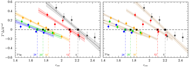
Figure 1: Interpolations of data from table 2 to $T^{\ast}\!\Delta M^{ud}=0$ individually at each $T^{\ast}\!/a$ (left), or using the global ansatz of eq. (5.34) (right). Results for $c_{\rm sw,I}$ are summarized in table 3.

	individual fit results				global fit results
$T^{\ast}\!/a$	$c_{\rm sw,I}$	$g_{0}^{2}$	$\kappa_{l}$	$\kappa_{\rm c}$	$c_{\rm sw,I}$	$g_{0}^{2}$	$\kappa_{l}$	$\kappa_{\rm c}$
$8$	$2.211(25)$	$1.8597$	$0.13450$	$0.11836$	$2.202(21)$	$1.8575$	$0.13459$	$0.11841$
$12$	$2.105(30)$	$1.8163$	$0.13482$	$0.12588$	$2.105(24)$	$1.8163$	$0.13482$	$0.12588$
$16$	$1.828(19)$	$1.7129$	$0.13640$	$0.12997$	$1.833(19)$	$1.7144$	$0.13636$	$0.12993$
$20$	$1.760(34)$	$1.6600$	$0.13619$	$0.13140$	$1.755(28)$	$1.6586$	$0.13623$	$0.13143$
$24$	$1.686(20)$	$1.6028$	$0.13605$	$0.13205$	$1.688(24)$	$1.6035$	$0.13603$	$0.13204$

Table 3: Interpolation results of $c_{\rm sw}^{\vphantom{()}}$ at $T^{*}M^{ud}=0$ for individual (local) and a global fit ansatz.

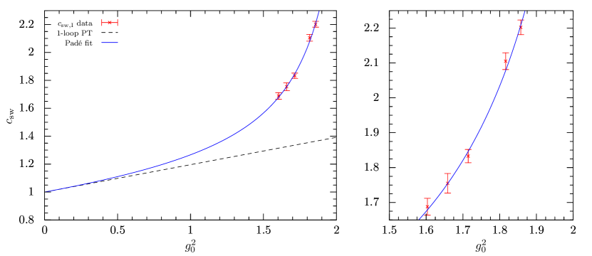
Figure 2: $c_{\rm sw,I}$ from global fit result as a function of the bare gauge coupling $g_{0}^{2}$, cf. eq. (5.36), along our line of constant physics.

We have determined the bare parameters for LCP lattices with $T=L$. To enhance the sensitivity to our improvement conditions we shall in the following however switch to the smaller spatial extent $L=T/2$ and asymmetric lattices. The $T/a$ values are unchanged to accommodate the various insertion time slices. The results for $M^{ud}$ and $\Delta M^{ud}$ on these lattices are listed in table 2. A glance at the last column shows that we have managed to bracket a zero of $\Delta M^{ud}T^{\ast}$ for each value $T^{\ast}\!/a$. To precisely locate the zeroes we use the following fit ansatz

$$T^{\ast}\Delta M^{ud}={\rm O}(a)=s\frac{a}{T^{\ast}}[c_{\rm sw}^{\vphantom{()}}-c_{\rm sw,I}(g_{0}^{2})]\,.$$ (5.34)

This fit is global in $T^{\ast}\!/a$ with one slope parameter $s$ and the improvement values $c_{\rm sw}^{\vphantom{()}}$ for each of our lattice sizes. It works very well with $s=-1.26(8)$ as seen in the right panel of figure 1. The corresponding bare parameters $g_{0}^{2},\kappa_{l\rm,I},\kappa_{\rm{\rm c},I}$ are determined by linearly interpolating the data in table 2. The resulting improvement values are compiled in table 3. In [21] it is discussed that fits of the type (5.34) with independent slopes for each $T^{\ast}\!/a$ lead to almost the same results. They are shown in the left panel of figure 1.

We now have a number of values $c_{\rm sw,I}$ for $c_{\rm sw}^{\vphantom{()}}$ that obey an improvement condition for five different values $g_{0}^{2}$ corresponding to $T^{\ast}\!/a=8,12,16,20,24$. In a last step we represent these data by a continuous fit function that interpolates between our ‘sampling’ points and matches the one-loop perturbative result [43]

$$c_{\rm sw}^{\vphantom{()}}=1+0.196g_{0}^{2}+{\rm O}(g_{0}^{4})\,,$$ (5.35)

for $g_{0}^{2}\to 0$. Our fit is given by the Padé form

$$c_{\rm sw,I}(g_{0}^{2}) =\frac{1+Ag_{0}^{2}+Bg_{0}^{4}}{1+(A-0.196)g_{0}^{2}}\,, A =-0.257\,, B =-0.050\,.$$ (5.36)

The fit parameters emerge with errors, of course, but at this point we neglect this and propose the fit formula as a definition of an O($a$) improved action. In figure 2 we see that the data are represented well. An initially used $g_{0}^{6}$ term in the numerator turned out not to be needed and receive a coefficient compatible with zero. In a few tests we finally have convinced [21] ourselves that the spreads that we have allowed in tuning the $\Phi_{i}^{\ast}$ are subdominant in the errors of the fitted $c_{\rm sw}^{\vphantom{()}}$.

6 Conclusion

We have emphasized that the large mass $m_{\rm c}$ of charmed quarks leads to lattice artefacts proportional to $am_{\rm c}\approx 0.5$ for presently attainable lattice spacings. In the usual setting of a mass independent renormalization scheme with O($a$) Symanzik improvement $am_{\rm c}$ appears in numerous improvement terms, which are an order more important than the analogous light quark terms. For unquenched charm even observables in the light quark sector are polluted by such cutoff effects.

We find it impractical to tune all corresponding coefficients precisely enough, but instead propose and design a scheme of renormalization and improvement conditions formulated at or close to the physical charm mass. With Schrödinger functional boundary conditions we introduce a renormalized coupling and effective meson masses that define a finite size scheme. Held fixed, they define a series of lattices where only the lattice spacing changes. We use them to compute the coefficient $c_{\rm sw}^{\vphantom{()}}(g_{0}^{2})$ of the clover improvement term. Our result is wrapped up in the formula (5.36) that we would like to advocate for use in future dynamical charm quark simulations.

Acknowledgements. We thank O. Bär and T. Korzec for input and discussions at an early stage of this project and P. Weisz for a critical reading of the manuscript. We are indebted to our colleagues in the ALPHA collaboration, especially those who worked on the code basis when this project started: S. Schaefer, H. Simma and A. Ramos for their modifications of the production code (an extension of openQCD v1.0 [51, 52]) and C. Wittemeier for the SFCF [53] code to measure SF correlation functions. Last but not least, the first determination of $c_{\rm sw}^{\vphantom{()}}$ along a line of constant physics would not have been possible without the generous computer support at HLRN (bep00040), NIC at DESY Zeuthen (PAX) and the AG COM at HU. This work was supported by the Deutsche Forschungsgemeinschaft in the SFB/TR 09.

References

- [1] K. G. Wilson, Confinement of Quarks , Phys.Rev. D10 (1974) 2445–2459.
- [2] H. B. Nielsen and M. Ninomiya, A no-go theorem for regularizing chiral fermions, Phys.Lett. B105 (1981) 219.
- [3] K. G. Wilson, Quarks and Strings on a Lattice, in New Phenomena in Subnuclear Physics: Proceedings, International School of Subnuclear Physics, Erice, Sicily, Jul 11-Aug 1 1975. Part A, p. 99, 1975.
- [4] B. Sheikholeslami and R. Wohlert, Improved Continuum Limit Lattice Action for QCD with Wilson Fermions, Nucl.Phys. B259 (1985) 572.
- [5] ETM collaboration, R. Baron et al., Light hadrons from lattice QCD with light (u,d), strange and charm dynamical quarks, JHEP 06 (2010) 111, [1004.5284].
- [6] ETM collaboration, N. Carrasco et al., Up, down, strange and charm quark masses with Nf = 2+1+1 twisted mass lattice QCD, Nucl. Phys. B887 (2014) 19–68, [1403.4504].
- [7] HPQCD, UKQCD collaboration, E. Follana, Q. Mason, C. Davies, K. Hornbostel, G. P. Lepage, J. Shigemitsu et al., Highly improved staggered quarks on the lattice, with applications to charm physics, Phys. Rev. D75 (2007) 054502, [hep-lat/0610092].
- [8] HPQCD collaboration, A. Hart, G. M. von Hippel and R. R. Horgan, Radiative corrections to the lattice gluon action for HISQ improved staggered quarks and the effect of such corrections on the static potential, Phys. Rev. D79 (2009) 074008, [0812.0503].
- [9] MILC collaboration, A. Bazavov et al., Scaling studies of QCD with the dynamical HISQ action, Phys. Rev. D82 (2010) 074501, [1004.0342].
- [10] A. X. El-Khadra, A. S. Kronfeld and P. B. Mackenzie, Massive fermions in lattice gauge theory, Phys. Rev. D55 (1997) 3933–3957, [hep-lat/9604004].
- [11] S. Aoki, Y. Kuramashi and S.-i. Tominaga, Relativistic heavy quarks on the lattice, Prog. Theor. Phys. 109 (2003) 383–413, [hep-lat/0107009].
- [12] J. Harada, A. S. Kronfeld, H. Matsufuru, N. Nakajima and T. Onogi, O(a) improved quark action on anisotropic lattices and perturbative renormalization of heavy-light currents, Phys. Rev. D64 (2001) 074501, [hep-lat/0103026].
- [13] J. Harada, S. Hashimoto, K.-I. Ishikawa, A. S. Kronfeld, T. Onogi and N. Yamada, Application of heavy quark effective theory to lattice QCD. 2. Radiative corrections to heavy-light currents, Phys. Rev. D65 (2002) 094513, [hep-lat/0112044], [Erratum-ibid. D71, 019903 (2005)].
- [14] J. Harada, S. Hashimoto, A. S. Kronfeld and T. Onogi, Application of heavy quark effective theory to lattice QCD. 3. Radiative corrections to heavy-heavy currents, Phys. Rev. D65 (2002) 094514, [hep-lat/0112045].
- [15] J. Harada, H. Matsufuru, T. Onogi and A. Sugita, Heavy quark action on the anisotropic lattice, Phys. Rev. D66 (2002) 014509, [hep-lat/0203025].
- [16] S. Aoki, Y. Kayaba and Y. Kuramashi, A Perturbative determination of mass dependent O(a) improvement coefficients in a relativistic heavy quark action, Nucl. Phys. B697 (2004) 271–301, [hep-lat/0309161].
- [17] S. Aoki, Y. Kayaba and Y. Kuramashi, Perturbative determination of mass dependent O(a) improvement coefficients for the vector and axial vector currents with a relativistic heavy quark action, Nucl. Phys. B689 (2004) 127–156, [hep-lat/0401030].
- [18] N. H. Christ, M. Li and H.-W. Lin, Relativistic Heavy Quark Effective Action, Phys.Rev. D76 (2007) 074505, [hep-lat/0608006].
- [19] H.-W. Lin and N. Christ, Non-perturbatively Determined Relativistic Heavy Quark Action, Phys.Rev. D76 (2007) 074506, [hep-lat/0608005].
- [20] M. B. Oktay and A. S. Kronfeld, New lattice action for heavy quarks, Phys. Rev. D78 (2008) 014504, [0803.0523].
- [21] F. Stollenwerk, Determination of in Lattice QCD with massive Wilson fermions. PhD thesis, Humboldt-Universität zu Berlin, Mathematisch-Naturwissenschaftliche Fakultät, 2017. [doi:10.18452/17706].
- [22] K. Symanzik, Some Topics in Quantum Field Theory, in Mathematical Problems in Theoretical Physics. Proceedings, 6th International Conference on Mathematical Physics, West Berlin, Germany, August 11-20, 1981, pp. 47–58, 1981. [doi:10.1007/3-540-11192-1_11].
- [23] K. Symanzik, Continuum Limit and Improved Action in Lattice Theories. 1. Principles and theory, Nucl.Phys. B226 (1983) 187.
- [24] K. Symanzik, Continuum Limit and Improved Action in Lattice Theories. 2. O(N) nonlinear sigma model in perturbation theory, Nucl.Phys. B226 (1983) 205.
- [25] M. Lüscher, S. Sint, R. Sommer and P. Weisz, Chiral symmetry and O(a) improvement in lattice QCD, Nucl.Phys. B478 (1996) 365–400, [hep-lat/9605038].
- [26] M. Lüscher and P. Weisz, On-Shell Improved Lattice Gauge Theories, Commun.Math.Phys. 97 (1985) 59.
- [27] T. Bhattacharya, R. Gupta, W. Lee, S. R. Sharpe and J. M. Wu, Improved bilinears in lattice QCD with non-degenerate quarks, Phys.Rev. D73 (2006) 034504, [hep-lat/0511014].
- [28] M. Lüscher, S. Sint, R. Sommer, P. Weisz and U. Wolff, Nonperturbative O(a) improvement of lattice QCD, Nucl.Phys. B491 (1997) 323–343, [hep-lat/9609035].
- [29] ALPHA collaboration, K. Jansen and R. Sommer, O(a) improvement of lattice QCD with two flavors of Wilson quarks, Nucl.Phys. B530 (1998) 185–203, [hep-lat/9803017], [Erratum-ibid. B643 (2002) 517].
- [30] CP-PACS & JLQCD collaboration, N. Yamada et al., Non-perturbative O(a)-improvement of Wilson quark action in three-flavor QCD with plaquette gauge action, Phys.Rev. D71 (2005) 054505, [hep-lat/0406028].
- [31] CP-PACS & JLQCD collaboration, S. Aoki et al., Non-perturbative O(a) improvement of the Wilson quark action with the RG-improved gauge action using the Schrödinger functional method, Phys.Rev. D73 (2006) 034501, [hep-lat/0508031].
- [32] QCDSF & UKQCD collaboration, N. Cundy et al., Non-perturbative improvement of stout-smeared three flavour clover fermions, Phys. Rev. D79 (2009) 094507, [0901.3302].
- [33] ALPHA collaboration, F. Tekin, R. Sommer and U. Wolff, Symanzik improvement of lattice QCD with four flavors of Wilson quarks, Phys.Lett. B683 (2010) 75–79, [0911.4043].
- [34] J. Bulava and S. Schaefer, Improvement of lattice QCD with Wilson fermions and tree-level improved gauge action, Nucl.Phys. B874 (2013) 188–197, [1304.7093].
- [35] M. Lüscher, R. Narayanan, P. Weisz and U. Wolff, The Schrödinger functional: A Renormalizable probe for non-Abelian gauge theories, Nucl.Phys. B384 (1992) 168–228, [hep-lat/9207009].
- [36] S. Sint, On the Schrödinger functional in QCD, Nucl.Phys. B421 (1994) 135–158, [hep-lat/9312079].
- [37] R. Narayanan and H. Neuberger, Infinite N phase transitions in continuum Wilson loop operators, JHEP 03 (2006) 064, [hep-th/0601210].
- [38] M. Lüscher, Properties and uses of the Wilson flow in lattice QCD, JHEP 1008 (2010) 071, [1006.4518].
- [39] Z. Fodor, K. Holland, J. Kuti, D. Nogradi and C. H. Wong, The Yang–Mills gradient flow in finite volume, JHEP 1211 (2012) 007, [1208.1051].
- [40] A. Ramos, The gradient flow running coupling with twisted boundary conditions, JHEP 1411 (2014) 101, [1409.1445].
- [41] P. Fritzsch and A. Ramos, The gradient flow coupling in the Schrödinger Functional, JHEP 1310 (2013) 008, [1301.4388].
- [42] ALPHA collaboration, M. Guagnelli, J. Heitger, R. Sommer and H. Wittig, Hadron masses and matrix elements from the QCD Schrödinger functional, Nucl. Phys. B560 (1999) 465–481, [hep-lat/9903040].
- [43] S. Aoki, R. Frezzotti and P. Weisz, Computation of the improvement coefficient to one loop with improved gluon actions, Nucl.Phys. B540 (1999) 501–519, [hep-lat/9808007].
- [44] ALPHA collaboration, P. Fritzsch, F. Knechtli, B. Leder, M. Marinkovic, S. Schaefer et al., The strange quark mass and Lambda parameter of two flavor QCD, Nucl.Phys. B865 (2012) 397–429, [1205.5380].
- [45] ALPHA collaboration, B. Blossier, M. Della Morte, P. Fritzsch, N. Garron, J. Heitger et al., Parameters of Heavy Quark Effective Theory from lattice QCD, JHEP 1209 (2012) 132, [1203.6516].
- [46] S. Duane, A. Kennedy, B. Pendleton and D. Roweth, Hybrid Monte Carlo, Phys. Lett. B195 (1987) 216–222.
- [47] A. D. Kennedy, I. Horvath and S. Sint, A New exact method for dynamical fermion computations with nonlocal actions, Nucl. Phys. Proc. Suppl. 73 (1999) 834–836, [hep-lat/9809092].
- [48] M. Clark and A. Kennedy, Accelerating dynamical fermion computations using the rational hybrid Monte Carlo (RHMC) algorithm with multiple pseudofermion fields, Phys.Rev.Lett. 98 (2007) 051601, [hep-lat/0608015].
- [49] ALPHA collaboration, M. Dalla Brida, P. Fritzsch, T. Korzec, A. Ramos, S. Sint and R. Sommer, Slow running of the Gradient Flow coupling from 200 MeV to 4 GeV in QCD, Phys. Rev. D95 (2017) 014507, [1607.06423].
- [50] P. Fritzsch and T. Korzec, “Simulating the QCD Schrödinger Functional with three massless quark flavors.” in preparation.
- [51] openQCD – Simulation program for lattice QCD, . http://luscher.web.cern.ch/luscher/openQCD/.
- [52] M. Lüscher and S. Schaefer, Lattice QCD with open boundary conditions and twisted-mass reweighting, Comput. Phys. Commun. 184 (2013) 519–528, [1206.2809].
- [53] C. Wittemeier, Implementation of a Program for QCD and HQET Correlation Functions in the Schrödinger Functional, Master’s thesis, Westfälische-Wilhelms Universität Münster, Mathematisch-Naturwissenschaftliche Fakultät, February, 2012.