Living Orthogonally: Quasi-universal Extra Dimensions

Abstract

The minimal Universal Extra Dimension scenario is highly constrained owing to opposing constraints from the observed relic density on the one hand, and the non-observation of new states at the LHC on the other. Simple extensions in five-dimensions can only postpone the inevitable. Here, we propose a six-dimensional alternative with the key feature being that the SM quarks and leptons are localized on orthogonal directions whereas gauge bosons traverse the entire bulk. Several different realizations of electroweak symmetry breaking are possible, while maintaining agreement with low energy observables. This model is not only consistent with all the current constraints opposing the minimal Universal Extra Dimension scenario but also allows for a multi-TeV dark matter particle without the need for any fine-tuning. In addition, it promises a plethora of new signatures at the LHC and other future experiments.

1 Introduction

Although the spectacular discovery of the long-sought for Higgs boson Aad:2012tfa ; Aad:2012an ; Chatrchyan:2012xdj is cited as the completion and the latest vindication of the Standard Model (SM), certain questions remain unanswered. These pertain to the existence of Dark Matter (DM), the origin of the baryon asymmetry in the Universe, the existence of multiple generations of fermions, the hierarchy in fermion masses and mixing, and, last but not the least, the stability of the Higgs sector under quantum corrections. The pursuit of answers to such questions has led to two different paradigms for the exploration of physics beyond the SM. The top to bottom approach posits a UV complete model, usually motivated to solve one or more of the outstanding problems (including the hierarchy), and delves into its “low-energy” consequences. Unfortunately, the most straightforward of them, whether it be supersymmetry or warped extra dimensions are faced with stringent constraints from observations. Hence, one is forced to consider non-minimal versions, an exercise that could, potentially, be non-intuitive on account of the lack of clear principles. The second, or bottom to top approach envisages simplified models, which while not addressing the UV scale physics, can explain certain anomalies in particle physics experiments (including but not limited to those at colliders) and possibly also cosmological observations.

Over the years, several attempts have been made to address the aforementioned questions, albeit only with partial success. One such stream of thought envisages a world in more than three space dimensions as a possible panacea to some of the ills of the SM, and, in this paper, we concentrate on this possibility. A particularly simplistic version was given the name Minimal Universal Extra Dimensions (mUED), wherein the SM is extended to propagate in a 5 dimensional space-time orbifolded to $M^{4}\otimes S^{1}/Z_{2}$, with $M^{4}$ being the four-dimensional space-time with Lorentz symmetry. If the radius of the fifth dimension be small enough, this leaves us with an effective 4-dimensional theory with every SM particle having a corresponding infinite tower of Kaluza Klein (KK) modes separated at equal energy gaps related to the inverse of the compactification scale.

Being an non-renormalizable model, mUED is considered as an effective theory valid up to a cut-off $\Lambda$, typically assumed to be 5–40 times the inverse radius. One of the main attractions of MUED was the fact that, while the conservation of the KK-number (or, in other words, the momentum in the compactified direction) is broken by quantum corrections, a $Z_{2}$ symmetry, called KK-parity, is maintained nevertheless. This has the consequence that the lightest of the level-1 KK partners (upon accounting for the radiative effects Cheng:2002iz , normally the cousin of the hypercharge gauge boson) is absolutely stable, thereby being a natural candidate for the Dark Matter particle Servant:2002aq ; Kong:2005hn ; Burnell:2005hm ; Kakizaki:2006dz ; Belanger:2010yx . This model has been studied in great detail, since it bore resemblance with the LHC signatures of the minimal supersymmetric standard model, except for the spin of the individual particles.

While the electroweak Baak:2011ze and flavour Haisch:2007vb ; Dey:2016cve observables impose only relatively weak bounds on the compactification scale, namely $R^{-1}\gtrsim 750\,{\rm GeV}$ and $R^{-1}\gtrsim 600\,{\rm GeV}$ respectively, the current LHC bounds are much stronger, and emanate from the study of a variety of final states Choudhury:2016tff ; Deutschmann:2017bth ; Beuria:2017jez , such as multijets, or dileptons with jets, each accompanied by missing transverse energy ($\cancel{E}_{T}$), owing to the presence of the lightest KK-particle. With $\Lambda R$ ($R$ being the compactification scale) determining the mass splittings, the detection efficiency (for a given $R^{-1}$) and, hence, the experimental reach is also determined by this. The excellent agreement of the ATLAS data (at 13 TeV) on dileptons ATLAS:2016xcm and multijets with a single-lepton ATLAS:2016lsr with the SM expectations, serves to exclude $R^{-1}\lesssim 1400\,{\rm GeV}$ (for $\Lambda R\gtrsim 10$) or $R^{-1}\lesssim 1500\,{\rm GeV}$ (for $\Lambda R\lesssim 10$) at 95% C.L.

On the other hand, the agreement of the consequent relic density with the WMAPKomatsu:2010fb or the Planck Ade:2015xua data demands that $1250\,{\rm GeV}\lesssim R^{-1}\lesssim 1500\,{\rm GeV}$ Belanger:2010yx . These two sets of results are in serious conflict with each other, and continuing validity of this model would require substantial alterations. The simplest solution, of course, would be to break KK-parity and give up on the DM-candidate. A more attractive proposition would be to somehow alter the spectrum so as to either suppress the relic abundance or relax the LHC constraints by raising the masses of the strongly interacting particles. A partial solution can be achieved by invoking perfectly-tuned brane localized and/or higher dimensional terms in the Lagrangian. While the existence of such terms is anticipated as the UED is only an effective field theory with a cutoff $\Lambda$, the symmetric character of such terms (necessary for stability of the DM) is to be assured by imposing a KK-parity. Attractive as this proposition might be, it only offers a partial solution as the twin constraints (LHC and relic density) would require rather large sizes for these terms, that, ostensibly, arise from quantum corrections.

While for reasons of simplicity (and on account of the constraints from electroweak observables being relatively mild in this case), most models have concentrated on a five-dimensional world, this, though, need not be the case. Indeed, the extension to six dimensions Burdman:2005sr ; Dobrescu:2004zi ; Maru:2009wu ; Cacciapaglia:2009pa ; Dohi:2010vc brings forth its own advantages, e.g., in the context of explaining the existence of three fermion generations, or the reconciliation with the non-observance of proton decay. On the other hand, the simplest generalization, typically, results in even stronger constraints from relic density Dobrescu:2007ec . Thus, smarter generalizations are called for. Embedding the UED in a 6-dimensional warped space Arun:2016csq ; Arun:2017zap , for example, makes it possible to evade the relic density bounds by exploiting the $s$-channel annihilation channel with graviton mediated by a KK-graviton exchange. In this paper we offer a different solution, one that leads to a very rich collider phenomenology.

The rest of this article is constructed as follows. We begin by setting up the formalism, followed by details of the model including the breaking of the electroweak symmetry and culminating with the Feynman rules. This is followed (in Sec. 4) by an examination of the mass-splittings wrought by quantum corrections. A detailed study of the relic abundance and the consequent constraints imposed on the parameter space of the theory is presented in Section 5. Also discussed are the prospects for direct and indirect detection experiments. An independent set of constraints arise from new particle searches at the LHC and these are discussed in Section 6. Finally, we conclude in Section 8 and list some open questions.

2 The Model

Consider a 6-dimensional flat space-time orbifolded on $M^{4}\otimes(S^{1}/Z_{2})\otimes(S^{1}/Z_{2})$ parametrized by the coordinates ($x_{\mu},x_{4},x_{5}$), where $M^{4}$ is the 4-dimensional space ($x_{\mu}$) that obeys Lorentz symmetry, and $x_{4,5}$ are compact and dimensionless. The line element for this space-time is given as,

$$ds^{2}=\eta_{\mu\nu}dx^{\mu}dx^{\nu}+R_{q}^{2}dx_{4}^{2}+r_{\ell}^{2}dx_{5}^{2}\ ,$$

where $R_{q}$ and $r_{\ell}$ are the compactification radii in the $x_{4}$ and $x_{5}$ directions respectively. The latter are orbifolded by individual $Z_{2}$’s, and periodic boundary conditions ($x_{4}\rightarrow x_{4}+\pi$ and $x_{5}\rightarrow x_{5}+\pi$) are assumed. This particular orbifolding demands the sides of the six-dimensional space to be protected by 4-branes (or 4+1 dimensional hyper surfaces). This feature is distinctively different from the toroidal orbifolding ($T^{2}/Z_{2}$) where the branes are present only at the corners and are co-dimension 2. It should be noted that it is the mutual independence of the two orbifoldings that allows for $R_{l}\neq r_{q}$, rendering the six-dimensional bulk spacetime to be different (similar spacetime has also been considered in Refs.Li:2001qs ; Li:2002xw ) from the chiral square Dobrescu:2004zi .

The key feature is that the SM quarks and leptons are extended not to the entire bulk, but only to orthogonal directions. Apart from other consequences (to be elaborated on later) this immediately decouples the inter-level mass splittings for quarks and leptons, thereby raising the possibility that the LHC bounds could be evaded while satisfying the constraints from relic abundance. To be specific, we consider the case where the lepton fields exist only on the 4-brane at $x_{4}=0$ while quarks exist, symmetrically, on a different set of 4-branes, at $x_{5}=0$ and $x_{5}=\pi$, that are orthogonal to the leptonic brane. This difference in the assignments of quarks and leptons has very important ramifications. As we shall see later, the symmetric assignation of the quark field will allow us to retain the $Z_{2}$ symmetry associated with the “leptonic direction”, viz. $x_{5}\to\pi-x_{5}$ , whereas the corresponding symmetry in the $x_{4}$ direction is manifestly lost. To remind us of this aspect (one which will have immense consequences), we will denote the remaining discrete symmetry of the model by $Z_{2}^{\ell}\otimes\cancel{Z}_{2}^{q}$ (where the slash denotes the explicit breaking). The free Lagrangian for the fermions is, then, given by

$$\begin{array}[]{rcl}S_{\rm fermion}&=&\displaystyle\int\int_{0}^{\pi}\int_{0}^{\pi}dx^{\mu}dx_{4}dx_{5}\,\left[\sqrt{g_{1}}{\cal L}_{q}\,\frac{\left\{\delta(x_{5})+\delta(x_{5}-\pi)\right\}}{2}+\sqrt{g_{2}}{\cal L}_{\ell}\,\delta(x_{4})\right]\\[8.61108pt] {\cal L}_{\ell}&\equiv&\displaystyle\bar{L}(-i\gamma^{\mu}\partial_{\mu}-i\gamma_{5}r_{\ell}^{-1}\partial_{5})L+\bar{E}(-i\gamma^{\mu}\partial_{\mu}-i\gamma_{5}r_{\ell}^{-1}\partial_{5})E\\[8.61108pt] {\cal L}_{q}&\equiv&\displaystyle\bar{Q}(-i\gamma^{\mu}\partial_{\mu}-i\gamma_{4}R_{q}^{-1}\,\partial_{4})Q+\bar{U}(-i\gamma^{\mu}\partial_{\mu}-i\gamma_{4}R_{q}^{-1}\,\partial_{4})U\\ &+&\displaystyle\bar{D}(-i\gamma^{\mu}\partial_{\mu}-i\gamma_{4}R_{q}^{-1}\,\partial_{4})D\end{array}$$ (1)

where $L/Q$ are the lepton/quark doublets and $E/U/D$ are the lepton/quark singlets and $\sqrt{g_{1}}=R_{q}$, $\sqrt{g_{2}}=r_{\ell}$. The fermions, being 5-dimensional, are vector like. The unwanted zero-mode chiral states can be projected out by orbifolding appropriately, viz., for $x_{5}\to-x_{5}$,

$$L(x_{\mu},x_{5})=\gamma^{5}L(x_{\mu},-x_{5})\ ,\hskip 5.0ptE(x_{\mu},x_{5})=-\gamma^{5}E(x_{\mu},-x_{5})$$

while for $x_{4}\rightarrow-x_{4}$,

$$Q(x_{\mu},x_{4})=\gamma^{5}Q(x_{\mu},-x_{4})\ ,\hskip 5.0ptU(x_{\mu},x_{5})=-\gamma^{5}U(x_{\mu},-x_{5})\ ,\hskip 5.0ptD(x_{\mu},x_{5})=-\gamma^{5}D(x_{\mu},-x_{5})\ .$$

The corresponding Fourier decompositions of the fermion fields are given by

$$\begin{array}[]{rcl}\sqrt{\pi r_{\ell}}\,L(x_{\mu},x_{5})&=&\displaystyle L_{l}^{(0,0)}(x_{\mu})+\sqrt{2}\;\sum_{p>0}\Big{(}L_{l}^{(0,p)}(x_{\mu})\cos\left(px_{5}\right)+L_{r}^{(0,p)}(x_{\mu})\sin\left(px_{5}\right)\Big{)}\\[6.45831pt] \sqrt{\pi r_{\ell}}\,E(x_{\mu},x_{5})&=&\displaystyle E_{r}^{(0,0)}(x_{\mu})+\sqrt{2}\;\sum_{p>0}\Big{(}E_{l}^{(0,p)}(x_{\mu})\cos\left(px_{5}\right)+E_{r}^{(0,p)}(x_{\mu})\sin\left(px_{5}\right)\Big{)}\\[6.45831pt] \sqrt{\pi R_{q}}\,Q(x_{\mu},x_{4})&=&\displaystyle Q_{l}^{(0,0)}(x_{\mu})+\sqrt{2}\;\sum_{n>0}\Big{(}Q_{l}^{(n,0)}(x_{\mu})\cos\left(nx_{4}\right)+Q_{r}^{(n,0)}(x_{\mu})\sin\left(nx_{4}\right)\Big{)}\\[6.45831pt] \sqrt{\pi R_{q}}\,U(x_{\mu},x_{4})&=&\displaystyle U_{r}^{(0,0)}(x_{\mu})+\sqrt{2}\;\sum_{n>0}\Big{(}U_{l}^{(n,0)}(x_{\mu})\cos\left(nx_{4}\right)+U_{r}^{(n,0)}(x_{\mu})\sin\left(nx_{4}\right)\Big{)}\\ \sqrt{\pi R_{q}}\,D(x_{\mu},x_{4})&=&\displaystyle D_{r}^{(0,0)}(x_{\mu})+\sqrt{2}\;\sum_{n>0}\Big{(}D_{l}^{(n,0)}(x_{\mu})\cos\left(nx_{4}\right)+D_{r}^{(n,0)}(x_{\mu})\sin\left(nx_{4}\right)\Big{)}\ .\end{array}$$ (2)

As expected, both the leptons and quarks have a single tower each. The former has only the $(0,p)$ modes with masses being given by $m_{\ell}^{(0,p)}=p\,r_{\ell}^{-1}$ where we have neglected the SM mass for the zero mode. The quarks, on the other hand, possess only the $(n,0)$ modes with masses $m_{q}^{(n,0)}=n\,R_{q}^{-1}$. Naively, one would expect that we would need $R_{q}^{-1}$ to be sufficiently larger than $r_{\ell}^{-1}$. However, as we shall see later, this requirement is not strictly true.

With quarks and leptons being extended in different directions, it is obvious that at least the electroweak gauge bosons must traverse the entire six-dimensional bulk. Before we delve into this, we offer a quick recount of the gauge sector in a generic higher-dimensional model.

2.1 Gauge Bosons: A lightning review

Naively, a five-dimensional gauge field, on compactification, should decompose into a four-dimensional vector field and an adjoint scalar, whereas for a six-dimensional field, there should be two such scalars instead. However, a simple counting of the degrees of freedom (especially for the KK-levels), shows immediately that, in each case, one of the scalar modes must vanish identically.

$x_{4}\rightarrow-x_{4},\quad x_{5}\rightarrow x_{5}$	$x_{4}\rightarrow x_{4},\quad x_{5}\rightarrow-x_{5}$
$A_{\mu}(x^{\mu},x_{4},x_{5})=A_{\mu}(x^{\mu},-x_{4},x_{5})$	$A_{\mu}(x^{\mu},x_{4},x_{5})=\displaystyle A_{\mu}(x^{\mu},x_{4},-x_{5})$
$A_{4}(x^{\mu},x_{4},x_{5})=-A_{4}(x^{\mu},-x_{4},x_{5})$	$A_{4}(x^{\mu},x_{4},x_{5})=A_{4}(x^{\mu},x_{4},-x_{5})$
$A_{5}(x^{\mu},x_{4},x_{5})=A_{5}(x^{\mu},-x_{4},x_{5})$	$A_{5}(x^{\mu},x_{4},x_{5})=-A_{5}(x^{\mu},x_{4},-x_{5})$
$\Theta(x^{\mu},x_{4},x_{5})=\Theta(x^{\mu},-x_{4},x_{5})$	$\Theta(x^{\mu},x_{4},x_{5})=\Theta(x^{\mu},x_{4},-x_{5})$

Table 1: Boundary conditions for the gauge fields.

To begin with, we look at the simpler abelian case and, then, graduate to the Standard Model gauge content. The action is given by

$$S=\int d^{4}x\int_{0}^{\pi}dx_{4}\int_{0}^{\pi}dx_{5}\,\sqrt{g}\left(-\frac{1}{4}F_{MN}F^{MN}+{\cal L}_{gf}\right)\ ,$$ (3)

where $\sqrt{g}=R_{q}r_{\ell}$ and $M,N=0,\dots,5$. To eliminate the spurious degrees of freedom corresponding to the gauge freedom, viz,

$$A_{M}(x^{N})\rightarrow A^{\prime}_{M}(x^{N})=A_{M}(x^{N})+\partial_{M}\Theta(x^{N})\ ,$$

we choose to work with the generalized $R_{\xi}$ gauge and

$${\cal L}_{gf}=-\frac{1}{2\xi}\left[\partial_{\mu}A^{\mu}-\xi\,(R_{q}^{-1}\partial_{4}A_{4}+r_{\ell}^{-1}\partial_{5}A_{5})\right]^{2}\ .$$ (4)

This has the further advantage of eliminating terms connecting $A_{\mu}$ to $A_{4,5}$. To compactify on the orbifold, we need to impose boundary conditions which are summarized in Table 1. We may, now, effect mode decomposition, viz.

$$\begin{array}[]{rcl}\pi\,\sqrt{R_{q}\,r_{\ell}}\,A_{\mu}(x^{\mu},x_{4},x_{5})&=&\displaystyle A^{(0,0)}_{\mu}(x^{\mu})+\sqrt{2}\,\sum_{j>0}A^{(j,0)}_{\mu}(x^{\mu})\;\cos\left(jx_{4}\right)\\ &+&\displaystyle\sqrt{2}\sum_{k>0}A^{(0,k)}_{\mu}(x^{\mu})\;\cos\left(kx_{5}\right)+2\,\sum_{j,k>0}A^{(j,k)}_{\mu}(x^{\mu})\;\cos\left(jx_{4}\right)\cos\left(kx_{5}\right)\\[4.30554pt] \pi\,\sqrt{R_{q}\,r_{\ell}}\,A_{4}(x^{\mu},x_{4},x_{5})&=&\displaystyle\sqrt{2}\,\sum_{j>0}A^{(j,0)}_{4}(x^{\mu})\;\sin\left(jx_{4}\right)+2\,\sum_{j,k>0}A^{(j,k)}_{4}(x^{\mu})\,\sin\left(jx_{4}\right)\cos\left(kx_{5}\right)\\[4.30554pt] \pi\,\sqrt{R_{q}\,r_{\ell}}\,A_{5}(x^{\mu},x_{4},x_{5})&=&\displaystyle\sqrt{2}\,\sum_{k>0}A^{(0,k)}_{5}(x^{\mu})\;\sin\left(kx_{5}\right)+2\,\sum_{j,k>0}A^{(j,k)}_{5}(x^{\mu})\,\cos\left(jx_{4}\right)\sin\left(kx_{5}\right)\ .\end{array}$$ (5)

The factor $\pi\,\sqrt{R_{q}r_{\ell}}$ serves to maintain canonical commutation relations for the KK components on compactification down to four dimensions. Clearly, $A_{4,5}^{(j,k)}$ transform as four-dimensional Lorentz scalars. Although, for $j,k\neq 0$, the kinetic terms mix the fields, these can be diagonalized provided we redefine them as

$$\begin{array}[]{rcl}V^{(j,k)}_{1}&=&\displaystyle\frac{1}{M_{j,k}}\,\left(\frac{k}{r_{\ell}}A^{(j,k)}_{4}-\frac{j}{R_{q}}A^{(j,k)}_{5}\right)\\ V^{(j,k)}_{2}&=&\displaystyle\frac{1}{M_{j,k}}\left(\frac{j}{R_{q}}A^{(j,k)}_{4}+\frac{k}{r_{\ell}}A^{(j,k)}_{5}\right)\end{array}$$ (6)

where, as usual, $M_{j,k}^{2}=j^{2}/R_{q}^{2}+k^{2}/r_{\ell}^{2}$. Under such a redefinition, after integrating out the extra dimensions, the effective four-dimensional Lagrangian density is

$$\begin{array}[]{rcl}{\cal L}&=&\displaystyle\sum_{j,k}\left[\frac{-1}{4}\,F^{(j,k)}_{\mu\nu}\,F^{(j,k)\mu\nu}+M^{2}_{j,k}\,A^{(j,k)}_{\mu}\,A^{(j,k)\mu}-\frac{1}{2\xi}(\partial_{\mu}A^{(j,k)\mu})^{2}\right]\\ &+&\displaystyle\sum_{j,k}\left[(\partial_{\mu}V^{(j,k)}_{1})^{2}-M^{2}_{j,k}V^{(j,k)2}_{1}+(\partial_{\mu}V^{(j,k)}_{2})^{2}-\xi M^{2}_{j,k}V^{(j,k)2}_{2}\right]\end{array}$$ (7)

Using Eq 5, it is trivial to see that $V_{1}$ does not exist if $j=0$ or $k=0$. This reflects the orbifolding we have in this geometry. Thus, we have a double Kaluza-Klein tower for a vector field along with a pair of charge-neutral scalars, with these being degenerate at every level. In the unitary gauge ($\xi\to\infty$), the scalars $V_{2}^{(j,k)}$ become non propagating and the only (real) scalar fields left are $V_{1}^{(j,k)}$. This disappearance of one tower of the adjoint scalars can be understood in terms of the appearance of the longitudinal modes for the corresponding gauge boson levels.

2.2 The complete field assignment

The decomposition for non-abelian gauge boson is identical to that for the abelian case discussed above, with the added complication of the self interactions and the ghost fields needed to consistently define the quantum theory. The gauge field is now expressible as $A_{M}=A_{M}^{a}\,t^{a}$, and the field strength tensor as

$$F_{MN}=\partial_{M}\,A_{N}-\partial_{N}\,A_{M}+g\,[A_{M},A_{N}]$$

where $t^{a}$ are the generators and $g$ the six dimensional coupling constant. Once again, the gauge Lagrangian is written as

$${\cal L}_{\rm kin}=\frac{-1}{4}\,tr(F_{MN}\,F^{MN})\ ,$$

apart from the gauge fixing and the ghost terms. For convenience, we separate $F_{MN}$ into three sets $F_{\mu\nu}$, $F_{4\mu}$, $F_{5\mu}$ and $F_{45}$ as in the abelian case, with the understanding that each continues to be a function of all six dimensions. The bilinear terms, on KK reduction give rise, in analogy with the abelian case, to double towers of gauge bosons as well as of a pair of scalars $V_{1,2}$ in the adjoint representation. Once again, in the unitary gauge, $V_{2}$ decouples entirely. We desist from expanding the Lagrangian further to include the ghosts etc, since that is not germane to the issues under consideration.

Since we want to decouple the compactification scales for the strongly-interacting particles from those having only electroweak interactions, we consider the gluons to exist only on the very same branes where the quarks are located. Thus, the Lagrangian for the gauge sector is given by

$$\begin{array}[]{rcl}{\cal L}_{Gauge}&=&\displaystyle-\frac{1}{4}B_{MN}B^{MN}-\frac{1}{4}W^{a}_{MN}W^{aMN}-\,\frac{1}{4}G^{\aleph}_{\bar{M}\bar{N}}G^{\aleph\bar{M}\bar{N}}\frac{\left[\delta(x_{5})+\delta(x_{5}-\pi)\right]}{2}\\ {\cal L}_{GaugeFix.}&=&\displaystyle\frac{-1}{2\xi}\left(\partial^{\mu}B_{\mu}-\xi(R_{q}^{-1}\partial_{4}B_{4}+r_{\ell}^{-1}\partial_{5}B_{5})\right)^{2}\\ &-&\displaystyle\frac{1}{2\xi}\left(\partial^{\mu}W^{a}_{\mu}-\xi(R_{q}^{-1}\partial_{4}W^{a}_{4}+r_{\ell}^{-1}\partial_{5}W^{a}_{5})\right)^{2}\\ &-&\displaystyle\frac{1}{2\xi}\left\{\partial^{\mu}G^{\aleph}_{\mu}-\xi(R_{q}^{-1}\partial_{4}G^{\aleph}_{4})\right\}^{2}\frac{\left[\delta(x_{5})+\delta(x_{5}-\pi)\right]}{2}\ ,\end{array}$$ (8)

where $\bar{M},\bar{N}=0,\dots,4$, $a=1,2,3$, $\aleph=1\dots 8$. While the mode decomposition for the electroweak gauge bosons would be analogous to that presented in the preceding section (we will discuss symmetry breaking shortly), that for the gluon is simpler and is given by

$$\sqrt{\pi R_{q}}G_{\mu}^{\aleph}(x,x_{4})=G_{\mu}^{\aleph(0,0)}(x)+\sqrt{2}\sum_{n>0}G_{\mu}^{\aleph(n,0)}(x)\cos(nx_{4})\ ,$$ (9)

namely a single tower with masses given by $n/R_{q}$. In the unitary gauge, expectedly, no adjoint scalar remains.

Before delineating the Feynman rules for the gauge interactions, it is mandatory that we precisely define the covariant derivatives for the fermions. This follows in the usual manner, namely,

$$\partial_{M}\to D_{M}\equiv\partial_{M}-i\,g_{1}\,B_{M}-i\,g_{2}\,W_{M}^{a}T^{a}-ig_{3}\,G_{M}^{\aleph}T^{\aleph},$$ (10)

with the understanding that $G_{5}$ vanishes identically (since both quarks and gluons exist only on two particular branes). Further, it is convenient to define the following symbols:

$$\begin{array}[]{rclcl}&&b_{\vec{j}}&\equiv&2^{-(\delta_{j_{1},0}+\delta_{j_{2},0}+\delta_{j_{3},0}+1)/2}\\ \delta_{l}(\vec{j})&=&\delta_{j_{1},j_{2},j_{3}}&\equiv&\delta_{j_{1}+j_{3}+j_{2},0}+\delta_{j_{1}+j_{3}-j_{2},0}+\delta_{j_{1}-j_{2}-j_{3},0}+\delta_{j_{1}+j_{2}-j_{3},0}\\ \delta_{r}(\vec{j})&=&\bar{\delta}_{j_{1},j_{2},j_{3}}&\equiv&-\delta_{j_{1}+j_{3}+j_{2},0}-\delta_{j_{1}-j_{2}-j_{3},0}+\delta_{j_{1}-j_{2}+j_{3},0}+\delta_{j_{1}+j_{2}-j_{3},0}\\ &&b^{\prime}_{\vec{j},\vec{k}}&\equiv&2^{-2-(\delta_{j_{1},0}+\delta_{j_{2},0}+\delta_{j_{3},0}+\delta_{j_{4},0}+\delta_{k_{1},0}+\delta_{k_{2},0}+\delta_{k_{3},0}+\delta_{k_{4},0})/2}\\ &&\delta^{(1)}_{j_{1},j_{2},j_{3},j_{4}}&\equiv&\delta_{j_{1}+j_{2}+j_{3}+j_{4},0}+\delta_{j_{1}+j_{2}+j_{3}-j_{4},0}+\delta_{j_{1}+j_{2}-j_{3}+j_{4},0}+\delta_{j_{1}+j_{2}-j_{3}-j_{4},0}\\[0.0pt] &&&+&\displaystyle\delta_{j_{1}-j_{2}+j_{3}+j_{4},0}+\delta_{j_{1}-j_{2}+j_{3}-j_{4},0}+\delta_{j_{1}-j_{2}-j_{3}+j_{4},0}+\delta_{j_{1}-j_{2}-j_{3}-j_{4},0}\end{array}$$ (11)

In terms of these, the gauge couplings can be expressed as in Tables 2 & 3.

$A_{\mu}^{(n_{1},p_{1})}Q^{(n_{2},0)}_{l/r}Q^{(n_{3},0)}_{l/r}$	$g\,b_{\vec{n}}\,\delta_{l/r}(\vec{n})\,2^{(1-\delta_{p_{1},0})/2}$, for even $p_{1}$ (0 otherwise)
$A_{\mu}^{(n_{1},p_{1})}L^{(0,p_{2})}_{l/r}L^{(0,p_{3})}_{l/r}$	$g\,2^{(1-\delta_{n_{1},0})/2}\,b_{\vec{p}}\,\delta_{l/r}(\vec{p})$
$\partial_{\nu}A_{\mu}^{a(n_{1},p_{1})}A^{\nu b(n_{2},p_{2})}A^{\mu c(n_{3},p_{3})}$	$\displaystyle\frac{g}{2}\,f^{abc}\,b_{\vec{n}}b_{\vec{p}}\,\delta_{l}(\vec{n})\,\delta_{l}(\vec{p})$
$A_{\mu}^{b(n_{1},p_{1})}A_{\nu}^{c(n_{2},p_{2})}A^{\mu d(n_{3},p_{3})}A^{\nu e(n_{4},p_{4})}$	$\displaystyle\frac{g^{2}}{4}\,f^{abc}f^{ade}\,b^{\prime}_{\vec{n},\vec{p}}\,\delta^{(1)}_{n_{1},n_{2},n_{3},n_{4}}\,\delta^{(1)}_{p_{1},p_{2},p_{3},p_{4}}$
$A_{\mu}^{(n_{1},p_{1})}A_{\mu}^{(n_{2},p_{2})}\ H\ H\$	$\frac{g^{2}}{2}\,[1+(-1)^{n_{1}+n_{2}}]\,[1+(-1)^{p_{1}+p_{2}}]$
$\bar{Q}^{(n_{1},0)}d_{r}^{(n_{2},0)}\ H\$	$\lambda_{d}\frac{[1+(-1)^{n_{1}+n_{2}}]}{2}$
$\bar{L}^{(0,p_{1})}e_{r}^{(0,p_{2})}\ H\$	$\lambda_{e}\frac{[1+(-1)^{p_{1}+p_{2}}]}{2}$

Table 2: Interactions of bulk gauge boson fields, fermions and Higgs field. $f^{abc}$ are the structure constants. The Lorentz structures are as in the SM. It should be noted that since the gluons are localized on the same brane as the quarks, they have only a single KK-tower and KK-number conserving interactions. Here we have considered Higgs localized on the four corners.

$A_{\mu}^{(n_{1},p_{1})}A_{\mu}^{(n_{2},p_{2})}\ H^{(n_{3},p_{3})}\ H^{(n_{4},p_{4})}\$	$\frac{g^{2}}{4}\,b^{\prime}_{\vec{n},\vec{p}}\,\delta^{(1)}_{n_{1},n_{2},n_{3},n_{4}}\,\delta^{(1)}_{p_{1},p_{2},p_{3},p_{4}}$
$\bar{Q}^{(n_{1},0)}d_{r}^{(n_{2},0)}\ H^{(n_{3},p_{3})}\$	$\lambda_{d}\,b_{\vec{n}}\,\delta_{l}(\vec{n})\,2^{(1-\delta_{p_{1},0})/2}$, for even $p_{1}$ (0 otherwise)
$\bar{L}^{(0,p_{1})}e_{r}^{(0,p_{2})}\ H^{(n_{3},p_{3})}\$	$\lambda_{e}\,2^{(1-\delta_{n_{1},0})/2}\,b_{\vec{p}}\,\delta_{l}(\vec{p})$

Table 3: Interactions of bulk gauge boson and fermion with Higgs field in the bulk.

3 Electroweak Symmetry Breaking

While the discussion so far has been rather straightforward, complications may arise when symmetry breaking is introduced. Several realizations of the Higgs sector is possible, each with its own distinctive consequences. We illustrate this now, beginning with what, naively, might seem the simplest choice, before graduating to one that not only is easier to work with, but also more viable phenomenologically.

3.1 Higgs at the corners

We begin with a particularly simple one, wherein the Higgs field is localized to 3-branes at the four corners of the rectangle that the compact space is. The corresponding Lagrangian is, then, given by

$${\cal L}_{H}=-\frac{1}{4}\left[\frac{1}{2}(D_{\mu}H)^{\dagger}(D^{\mu}H)+V(H^{\dagger}H)\right]\,\left[\delta(x_{4})+\delta(x_{4}-\pi)\right]\,\left[\delta(x_{5})+\delta(x_{5}-\pi)\right].$$ (12)

A nontrivial vacuum expectation value for $H$ breaks the electroweak symmetry down to $U(1)_{\rm em}$. The very presence of the $\delta$-functions in ${\cal L}_{H}$ has an interesting consequence in that non-diagonal mass terms connecting the even and odd gauge boson modes, separately, are engendered. As a result, the physical $W$– and $Z$–bosons will have an admixture of all the even KK-modes . The mixings would be suppressed, though, by factors of the order of $g^{2}v^{2}/M_{KK}^{2}$ where $v$ is the electro-weak scale and $g$ the coupling constant.

The Yukawa coupling is as usual, namely

$${\cal L}_{\rm Yuk.}=\lambda_{u}\,\bar{Q}\,u_{r}\,(i\sigma^{2}H^{*})+\lambda_{d}\,\bar{Q}\,d_{r}\,H+\lambda_{e}\,\bar{L}\,e\,H\ .$$ (13)

The particular localization of the Higgs (as in eq.(12)) implies that, of the various fermion excitations, only the left-handed $SU(2)_{L}$-doublets and right-handed singlets couple to the Higgs. The wavefunctions for the other (wrong) chiralities vanish identically at the corners—see eq.(2)—which constitutes the only support of the Higgs. The existence of non-diagonal (in the level space) Yukawa as well as gauge couplings, both resulting from the localization of the Higgs on co-dimension 2 branes, has an immense bearing on the stability of the Higgs potential. Quantum corrections to the quartic Higgs vertex now emanate from a plethora of diagrams, with the negative contributions from the multitude of top (and top-cousin) loops, each proportional to $\lambda_{t}^{4}$, thereby, quickly destabilizing the potential. The larger multitude of diagrams, potentially, renders the problem even worse than that within the mUED Datta:2012db . Consequently, the cutoff $\Lambda$ needs to be relatively low.

Furthermore, this scenario leads to a computational problem in that the calculation of the gauge-boson wave functions is rendered very complicated. While a product such as $\delta(x_{4})\,\delta(x_{5})$ is best handled by going over to polar coordinates, this method fails here, not only on account of the lack of a spherical symmetry, but also as we have to deal with four such products. One could, still, adopt such a method in neighborhoods around each corner, and then sew them together. This, however, is not very illuminating. An added consequence is that the consequent changes in the gauge-boson wavefunctions (which, naturally, depend on the ratio of the symmetry-breaking-generated term and the compactification radii) lead to significant modifications of their couplings with the fermion zero-modes.

A way out of such problems would be to allow the Higgs to propagate in the bulk or even just the branes containing the quarks. This would imply that, as far as the tree-level Yukawa interactions (in particular, the ones involving the top-sector) are concerned, KK-number is now, rendered a good symmetry. These vertices being level-diagonal greatly reduces the number of fermion (top) loops contributing to the Higgs quartic coupling, postponing any instability to much higher energies.

3.2 Higgs on the quark branes

We discuss next the possibility that the Higgs are localized on the two 4-branes at $x_{5}=0,\pi$. Apart from the fact that, in the effective four-dimensional theory, there is now a tower of scalars instead of just the one, there is a further important change. The equations of motion for the gauge bosons, now, include two delta-functions, at $x_{5}=0,\pi$ respectively. While the solution thereof is straightforward, a key point needs to be appreciated. Although the scale of electroweak symmetry breaking is small compared to the Kaluza-Klein scale, the former cannot be treated as a simple perturbation as the solution space in the presence of a delta-function potential is different from that without. In particular, the characteristics of the gauge boson ground state changes radically, thereby leading to potentially large phenomenological changes.

The problem can be ameliorated if, instead of infinitesimally thin branes (as we have been assuming so far), we consider, instead, fat branes. This would lead to, amongst other changes, the tempering of the delta-function, and, as can be ascertained without much effort, the ground state would receive corrections of ${\cal O}(m_{W}^{2}R_{q}^{2})$ without destroying any of the important properties.

To execute such a possibility, we need to trap matter at specific locations in space. An exceedingly simple mechanism was discussed in Rubakov:1983bb and all we need is a confining potential such that a threshold energy is required to escape from the potential well. Such a potential, for example could be formed by kinks in a scalar theory.

3.2.1 Kinks in six dimensions

Consider a real scalar field $\chi$ with a Lagrangian given by coleman

$${\cal L}=\frac{1}{2}\,\partial^{M}\chi\,\partial_{M}\chi-V(\chi)\ ,\qquad V(\chi)=\frac{1}{2\,m^{2}\,a}\ \left[a\,\chi^{2}-m^{4}\right]^{2},$$ (14)

where $a$ is a positive constant and $M=0,\dots,5$. Thus, the self-coupling is $a/m^{2}$. Although ${\cal L}$ is invariant under the $Z_{2}$ symmetry $\chi\to-\chi$, the two degenerate minima, viz. $\chi=\pm m^{2}/\sqrt{a}$, evidently do not respect this $Z_{2}$. As is well-known, if a potential admits degenerate vacua, nontrivial time independent solutions to the equation of motion exist. While many different and inequivalent kink solutions are possible, it is the boundary conditions that dictate the appropriate one. Concentrating on classical solutions that are nontrivial only along the $x_{5}$ direction, we have

$$r_{\ell}^{-1}\,\partial_{5}\,\chi(x)=\left[-2\,V(\chi)\right]^{1/2}$$

leading to

$$\chi_{cl}(x_{5})=\pm\frac{m^{2}}{\sqrt{a}}\,\tanh\left(\frac{m\,r_{\ell}\,x_{5}}{\sqrt{2}}\right).$$ (15)

Henceforth, we refer to the positive (negative) sign as the kink (antikink) solutions. The energy of each is given by

$$E_{\rm kink}=r_{\ell}\,\int dx_{5}[\partial_{5}\chi_{cl}(x_{5})]^{2}=\int{d\chi}\,[-2V(\chi_{cl})]^{1/2}=\frac{\sqrt{2}\,m^{5}}{a}.$$ (16)

The modes about the kink solution can be obtained by effecting a perturbative expansion about it, namely $\chi(x^{M})=\chi_{cl}(x_{5})+\tilde{\chi}(x^{M})$. Linearizing the equation of motion for $\tilde{\chi}(x^{M})$, we have

$$\left[\partial_{M}\partial^{M}-m^{2}+\frac{3\,a}{m^{2}}\,\chi^{2}_{cl}\right]\tilde{\chi}=0.$$

If we want to interpret this in terms of five-dimensional modes, we must re-express $\tilde{\chi}$ as

$$\tilde{\chi}(x^{M})=\sum_{i}\chi_{i}(x^{\bar{M}})\,\eta_{i}(x_{5}),$$ (17)

where $\bar{M}=0,\dots,4$ and $\eta_{i}(x_{5})$ form an orthonormal basis. The equation of motion, then, simplifies to

$$\eta_{i}(x_{5})\,\partial_{\bar{M}}\partial^{\bar{M}}\chi_{i}(x^{\bar{M}})-\chi_{i}(x^{\bar{M}})\,\left[r_{\ell}^{-2}\,\partial_{5}^{2}+m^{2}-\,\frac{3\,a}{m^{2}}\,\chi^{2}_{cl}\right]\eta_{i}(x_{5})=0,$$

where $\bar{M}=0,1,2,3,4$, and $\eta_{i}(w)$ form orthonormal basis. Clearly, $\eta_{i}(x_{5})$ has to be an eigenfunction of the differential operator contained in the brackets. This is more conveniently expressed in terms of a rescaled dimensionless variable $z\equiv m\,r_{\ell}\,x_{5}/\sqrt{2}$, to yield

$$\left[-\partial_{z}^{2}-2+6\,\tanh^{2}(z)\right]\eta_{i}(z)=\frac{2\,\omega_{i}}{m^{2}}\,\eta_{i}$$ (18)

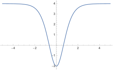
Figure 1: potential due to scalar field symmetry breaking to the equation $6\tanh[z]^{2}-2$.

This is but a one-dimensional Schrödinger equation for a potential as depicted in Fig. 1. Indeed, this is a particular example of a general class of potentials $U_{\ell}(z)\equiv\ell\,(\ell+1)\,\tanh^{2}z-2$. The problem is well studied DamienP.George:2009crn and the spectrum contains exactly $\ell$ discrete states with a continuum beyond.

3.2.2 Higgs localization

The simplest lagrangian for the doublet Higgs $H$ including a $Z_{2}$–invariant interaction with the bulk kink field $\chi$ can be written as

$$\begin{array}[]{rcl}{\cal L}_{scalar}&=&\displaystyle\frac{1}{2}(\partial_{M}\chi)\,(\partial^{M}\chi)-V(\chi)+\frac{1}{2}(D^{M}H)(D_{M}H^{\dagger})-\,\frac{1}{2}M_{H}^{2}(H^{\dagger}H)\\[8.61108pt] &+&\displaystyle\frac{a}{2m}g_{H\chi}(g_{H\chi}+1)\chi^{2}|H|^{2}\end{array}$$ (19)

where $m$ is the mass of the kink field. The equation of motion for the free Higgs field, in the $\chi_{\rm cl}$ background, is then

$$\Big{(}-\partial_{\bar{M}}\partial^{\bar{M}}-r_{\ell}^{-2}\partial_{5}^{2}+\frac{a}{m}g_{H\chi}(g_{H\chi}+1)\chi_{\rm cl}^{2}+M_{H}^{2}\Big{)}H=0\ .$$

Writing the Higgs field as

$$H(x_{\mu},x_{4},x_{5})=\sum_{p}H^{(p)}(x_{\mu},x_{4})f_{p}(x_{5})$$ (20)

where $f_{p}(x_{5})$ are a set of orthonormal functions, we get,

$$\Big{(}-M_{p}^{2}-r_{\ell}^{-2}\partial_{5}^{2}+\frac{1}{m}ag_{H\chi}(g_{H\chi}+1)\chi_{\rm cl}^{2}+M_{H}^{2}\Big{)}f_{p}=0\ ,$$ (21)

where we consider $H^{(p)}$ to be solutions of $\partial_{\bar{M}}\partial^{\bar{M}}H^{(p)}=M_{p}^{2}H^{(p)}$. Taking the classical configuration for the kink field, $\chi_{cl}=\sqrt{m^{3}/a}\,\tanh(m\,r_{\ell}\,x_{5}/\sqrt{2})$, the solution to the first bound state of the above equation with mass $M_{0}^{2}=M_{H}^{2}+\frac{1}{2}m^{2}g_{H\chi}$ is found to be

$$f_{0}=A_{0}\cosh^{-g_{H\chi}}\left(\frac{m\,r_{\ell}\,x_{5}}{\sqrt{2}}\right)$$ (22)

For $g_{H\chi}=1$, there exists only one bound state and the solution becomes

$$f_{0}={\rm sech}\left(\frac{m\,r_{\ell}\,x_{5}}{\sqrt{2}}\right)$$

and could be considered as Higgs for $M_{H}^{2}+\frac{1}{2}m^{2}g_{H\chi}=(125\,{\rm GeV})^{2}$.

Once the geometry is compactified, we need a system with kink and an anti-kink forming the domain walls at the boundaries of the orbifold. This leads to the symmetric space we have along the $x_{5}$ direction. Since the Higgs Lagrangian is symmetric with respect to the kink and anti-kink, the localization of Higgs would occur in the same way on both the domain walls. Hence the bound state of Higgs would have the wave function

$$f_{0}=\frac{1}{2}\left[{\rm sech}\left(\frac{m\,r_{\ell}\,x_{5}}{\sqrt{2}}\right)+{\rm sech}\left(\frac{m\,r_{\ell}\,(\pi-x_{5})}{\sqrt{2}}\right)\right].$$

Taking $m\rightarrow\infty$ we get back the delta function localization of Higgs field. Analogous mechanisms exist for fermion localization. We, however, will not dwell further on this mechanism as the phenomenological ramifications, in some sense, lie in between the two other choices of electroweak symmetry breaking.

3.3 Bulk Higgs

Allowing the Higgs field to propagate in the entire bulk, while leading to an additional profusion of fields in the four-dimensional limit (in the form of a tower of towers of scalars), is actually the simplest, of the three cases, to handle. The Lagrangian for this case is given by

$$S=\int d^{4}x\int_{0}^{\pi}dx_{4}\int_{0}^{\pi}dx_{5}\,\sqrt{g}\left[(D_{M}H)^{\dagger}(D^{M}H)+V(H^{\dagger}H)\right]$$ (23)

where

$$D_{M}=\partial_{M}-i\,g_{1}\,B_{M}-i\,g_{2}\,W_{M}^{a}T^{a}$$

and $V(H^{\dagger}H)=-\mu^{2}\,H^{\dagger}H+\lambda\,(H^{\dagger}H)^{2}$. The mode expansion is straightforward, namely,

$$\begin{array}[]{rcl}\pi\,\sqrt{R_{q}\,r_{\ell}}\,H(x^{\mu},x_{4},x_{5})&=&\displaystyle H^{(0,0)}(x^{\mu})+2\,\sum_{j,k>0}H^{(j,k)}(x^{\mu})\;\cos\left(jx_{4}\right)\cos\left(kx_{5}\right)\\ &+&\displaystyle\sqrt{2}\sum_{k>0}H^{(0,k)}(x^{\mu})\;\cos\left(kx_{5}\right)+\sqrt{2}\,\sum_{j>0}H^{(j,0)}(x^{\mu})\;\cos\left(jx_{4}\right)\end{array}$$ (24)

Only the $H^{(0,0)}$ Higgs doublet develops a vacuum expectation value, namely $H^{(0,0)}=(0,v/\sqrt{2})$ and the zero modes of both the electroweak gauge bosons and the Higgs boson acquire masses just as in the SM. The higher modes (including the charged higgs and pseudoscalar states) too mix within a given level, but with far smaller angles, owing to the hierarchy between the electroweak scale and the compactification scales. The mechanism is similar to that operative in the mUED caseCorderoCid:2011ja , albeit with additional complications.

The Yukawa lagrangian is given by

$$\begin{array}[]{rcl}S&=&\displaystyle\int d^{4}x\int_{0}^{\pi}dx_{4}\int_{0}^{\pi}dx_{5}\,\sqrt{g}\,\Bigg{\{}\left[\lambda_{u}\,\bar{Q}\,u\,(i\sigma^{2}H^{*})+\lambda_{d}\,\bar{Q}\,d\,H\right]\left[\frac{\delta(x_{5})+\delta(x_{5}-\pi)}{2}\right]\\[8.61108pt] &&\displaystyle\hskip 100.00015pt+\lambda_{e}\,\bar{L}\,e\,H\,\delta(x_{4})\Bigg{\}}\ ,\end{array}$$ (25)

where, for the sake of simplicity, we have suppressed the generational indices. With the fermions acquiring masses via boundary localized terms, there would exist mixings between the wavefunctions. However, this mixing is, understandably, small except for the case of the top quark. We shall not dwell on this aspect any further.

4 Quantum Corrections to the Spectrum

As we have seen in the preceding sections, with the quarks being localized symmetrically on the pair of end-of-world 4-branes at $x_{5}=0$ and $x_{5}=\pi$, there exists a $Z_{2}$ symmetry, namely $x_{5}\to\pi-x_{5}$. This is reflected by the corresponding wavefunctions being either symmetric (even $p$) or antisymmetric (odd $p$) about $x_{5}=\pi/2$. This $Z_{2}^{\ell}$ is analogous to the KK-parity in mUED, but operative only on modes along the $x_{5}$-direction. On the other hand, with the leptons being localized on the 4-brane at $x_{4}=0$ alone, the corresponding symmetry in this direction is lost entirely. Thus, while the lightest of the ${\cal F}^{(0,1)}$ particles (where ${\cal F}$ is an arbitrary field in the theory) is stable, this is not true for the ${\cal F}^{(1,0)}$.

The identification of the lightest of the level-1 excitations in either direction proceeds quite analogously to that in mUED. At the tree-level, the level-$(0,1)$ leptons and the $B_{\mu}^{(0,1)}$ are nearly degenerate. In the other direction, the level-$(1,0)$ partners of the light quarks are nearly degenerate with $B_{\mu}^{(1,0)}$ and $G_{\mu}^{(1,0)}$. However, quantum corrections lift these degeneracies. The corrections turn out to be small and negative for the $B_{\mu}$-cousins, and positive for the others. The extent of this splitting grows with the cutoff scale $\Lambda$.

While, within mUED, it has been argued that the stability of electroweak vacuumBhattacharyya:2006ym dictates $\Lambda\leq 4\,R^{-1}$, this constraint is not strictly applicable here. Vertices like $\bar{t}^{(n,0)}\,t^{(m,0)}\,H$ introduce additional box diagrams which tend to drive the effective Higgs self-coupling negative, thereby tending to destabilize the vacuum. These are only partially offset by the contributions from the $W^{(n,m)}$ (and $Z^{(n,m)}$) loops. The problem, however, is ameliorated to a great extent by allowing the Higgs to traverse the entire quark brane (thereby eliminating $\bar{t}^{(n,0)}\,t^{(m,0)}\,H^{(0,0)}$ vertices for $n\neq m$) instead of localizing it to the corners. To be conservative, we take heart from the fact that $\Lambda\sim 3\,\max(R_{q}^{-1},r_{\ell}^{-1})$ is a choice quite safe, irrespective of the realization of EWSB, from the viewpoint of Higgs stability, and we adopt this in this paper. To ease comparison with the literature (pertaining to mUED) we also demonstrate results for a case with a different choice as well, namely, $\Lambda=20\,\max(R_{q}^{-1},r_{\ell}^{-1})$.

Masses	Quantum Correction
$m_{Q}$	$\displaystyle M\,\left[1+\left(3\,a_{3}+\frac{27}{16}\,a_{2}+\frac{1}{16}\,a_{1}\right)\mathbb{L}\right]$
$m_{u}$	$\displaystyle M\,\left[1+\left(3\,a_{3}+\,a_{1}\right)\mathbb{L}\right]$
$m_{d}$	$\displaystyle M\,\left[1+\left(3\,a_{3}+\frac{1}{4}\,a_{1}\right)\mathbb{L}\right]$
$m_{L}$	$\displaystyle M\,\left[1+\left(\frac{27}{16}\,a_{2}+\frac{9}{16}\,a_{1}\right)\mathbb{L}\right]$
$m_{e}$	$\displaystyle M\,\left[1+\frac{9}{4}\,a_{1}\mathbb{L}\right]$
$m^{2}_{B_{(0,n)}}$	$\displaystyle M^{2}\,\left[1-\frac{a_{1}}{6}\,\mathbb{L}-\frac{17\,a_{1}}{2\,\pi^{2}}\,\zeta(3)\right]$
$m^{2}_{W_{(0,n)}}$	$\displaystyle M^{2}\,\left[1+\frac{15}{2}\,a_{2}\mathbb{L}+\frac{a_{2}}{2\,\pi^{2}}\,\zeta(3)\right]$
$m^{2}_{B_{(n,0)}}$	$\displaystyle M^{2}\,\left[1-\frac{a_{1}}{6}\,\mathbb{L}-\frac{21\,a_{1}}{2\,\pi^{2}}\,\zeta(3)-8\,a_{1}\,\mathbb{L}+\frac{m_{h}^{2}}{2M^{2}}\,a_{2}\,\mathbb{L}\right]$
$m^{2}_{W_{(n,0)}}$	$\displaystyle M^{2}\,\left[1+\frac{15}{2}\,a_{2}\mathbb{L}+\frac{a_{2}}{2\,\pi^{2}}\,\zeta(3)-4\,a_{2}\,\mathbb{L}+\frac{m_{h}^{2}}{2\,M^{2}}\,a_{2}\,\mathbb{L}\right]$
$m^{2}_{G}$	$\displaystyle M^{2}\,\left[1+\frac{23}{2}\,a_{3}\mathbb{L}-\frac{3\,a_{3}}{2\,\pi^{2}}\,\zeta(3)\,\right]$
$m^{2}_{H_{(0,n)}}$	$\displaystyle M^{2}\,\left[1+\frac{3}{4}\,a_{1}\mathbb{L}+\frac{3}{2}\,a_{2}\mathbb{L}-\frac{\lambda}{16\pi^{2}}\mathbb{L}\,\right]$
$m^{2}_{H_{(n,0)}}$	$\displaystyle M^{2}\,\left[1+\frac{3}{4}\,a_{1}\mathbb{L}+\frac{3}{2}\,a_{2}\mathbb{L}-\frac{\lambda}{16\pi^{2}}\mathbb{L}\,\right]$

Table 4: The one-loop corrections to the the masses of the KK excitations. In each case, $M$ refers to the corresponding tree-level masses.

The mass corrections can be separated into two primary classes, namely those due to bulk corrections and that due to the orbifolding. Though the calculations are quite straightforward Cheng:2002iz ; Freitas:2017afm , care must be taken of the fact that, in the present case, additional contributions accrue on account of non-diagonal couplings. It is useful to define

$$a_{i}\equiv\frac{g_{i}^{2}}{16\,\pi^{2}}\ ,\quad\mathbb{L}\equiv\ln\frac{\Lambda^{2}}{\mu^{2}}\ ,$$ (26)

where $g_{i}$ are the (4-dimensional) gauge coupling constants and $\mu$ is the renormalization scale. In terms of these, the masses are as given in Table 4. The terms proportional to the Riemann $\zeta(3)$ function denote the correction due to the orbifolding, while the rest are due to the various loops. Of particular interest are the terms $8\,a_{1}\,\mathbb{L}$ ($4\,a_{2}\,\mathbb{L}$) pertaining to $B_{\mu}^{(n,0)}$ ($W_{\mu}{a\,(n,0)}$). Appearing on account of the non-diagonal coupling of these bosons to lepton-pairs (originating, in turn, due to the broken $Z_{2}^{q}$), these terms have no counterpart in mUED scenarios. These corrections are quite significant (and, indeed are the dominant ones for $B_{\mu}^{(n,0)}$) leading to enhanced mass-splitting between particles of the same order.

The hypercharge-boson excited states $B_{\mu}^{(1,0)}$ and $B_{\mu}^{(0,1)}$ are, thus, the lightest excitations in the respective directions. The latter, being stable, is the DM candidate, while the former decays promptly and, predominantly, to the SM leptons. It is interesting to note that, in the event of $r_{\ell}\approx R_{q}$, the DM candidate is actually the heavier of the two.

5 The Dark Side

5.1 The Relic Density

Given the smallness of the mass splittings, in the early universe, the DM particle and the next-to-lightest KK particles would have decoupled around the same epoch. This can affect the relic abundance of DM in three ways. Before we list these, though, it should be pointed out that, contrary to mUED-like scenarios, not all KK-excitations of similar masses behave similarly. While the excitations along the leptonic ($x_{5}$) direction behave analogously to the NLKPs of mUED-like scenarios, it is the next-to-lightest lepton-direction excitations (NLLE) that are germane to the issue with the rest of the NLKPs (relevant only if $R_{q}\approx r_{\ell}$) playing a subservient role. With this understanding,

• NLLEs, after decoupling from the thermal bath, would decay to the lightest KK excitation i.e., the DM, thereby increasing the latter’s number density.

• The NLLEs would also have been interacting with the other SM particles before they decoupled, to replenish the DM and can keep the DM in equilibrium a little longer, thereby diluting their number density.

• Similarly, the NLLEs could also co-annihilate with the DM—to a pair of SM particles—again maintaining it (and themselves) in equilibrium longer.

The net effect would be determined by a complicated interplay of all such effects. A key issue is whether the NLLE decouples from the SM sector at or before the same epoch as the DM, or significantly later. In the latter case, the number density of the NLLE at the epoch of its own decoupling may be well below that of the DM, leading to only low levels of replenishment. In such a situation, it is often the second effect above that wins the day. Note that this is quite in contrast with the case of the mUED, where the inclusion of the co-annihilation channels increases the relic abundance thereby strengthening the upper bound on $R^{-1}$. This aspect would prove to be crucial in the context of our model.

To compute the relic density, we have implemented our model with the interactions discussed in section 2 in micrOMEGAsBelanger:2013oya using LanHEPSemenov:2014rea . As a check, we have compared against the CalcHEP model file discussed in Ref. Belyaev:2012ai . Care must be taken while calculating the relic density in micrOMEGAs. To produce the plot in Fig.2, we have considered upto four KK levels thereby requiring the modification of the array size used in micrOMEGAs.

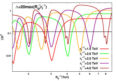
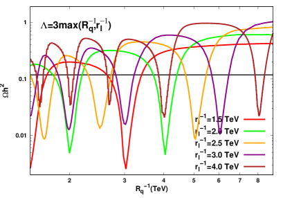
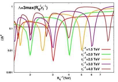
Figure 2: $\Omega h^{2}$ as a function of $R_{q}^{-1}$ for different values of $r_{\ell}^{-1}$. (a) and (b) correspond to differing values of the cutoff $\Lambda$ for the case when Higgs is localized at the 4 corners. (c) corresponds to the bulk Higgs scenario.

The resultant behavior of $\Omega h^{2}$ as a function of $R_{q}^{-1}$ is depicted in Fig.2. To understand the plots, several issues need to be appreciated. We examine these in turn, concentrating first on the case of the Higgs located at the corners. With fewer particles in the play, this case is easier to understand, at least as far as the relic density is concerned.

• In mUED-like scenarios, there are a plethora of particles nearly degenerate with the DM. While their co-annihilation with the DM serves to drive down the latter’s relic density, this is more than offset by the twin effects of $(a)$ these interacting with the SM particles prior to decoupling so as to replenish the DM and keep it in equilibrium for a longer while, and $(b)$ once decoupled, these decay into the DM, thereby enhancing the latter’s relic density. Overall, the existence of these particles serve to increase $\Omega_{DM}\,h^{2}$.

  In the present context, the excitations in the hadronic direction ($x_{4}$) play essentially no role in the aforementioned processes. Thus, one would expect the extent of the enhancement to be smaller.

• A further crucial difference emanates from our having confined the Higgs field to the corners of the brane-box. Consequently, there are no Higgs KK-excitations. Within the mUED, the second-level excitations appear as $s$-channel propagators in processes such as $B_{\mu}^{(1)}B_{\mu}^{(1)}\to H^{0(2)}\to t^{(0)}\bar{t}^{(0)}$ and $B_{\mu}^{(1)}H^{+(1)}\to H^{+(2)}\to t^{(0)}\bar{b}^{(0)}$, with the fermionic vertices being generated at one-loop order. The suppression due to the loop factor is offset by the fact of these processes occurring close to resonance. (Note that the reverse process is not nearly as efficient.)

  With the absence of the Higgs-excitations in our model, this means of suppression of the relic density is no longer available.

• Overall, then, one would imagine that the relic density should depend on the mass of the DM particle ($\sim r_{\ell}^{-1}$) in much the same way as in the mUED (i.e when Higgs-excitations are not included). This naive expectation does describe the situation well for $R_{q}^{-1}\gg r_{\ell}^{-1}$ (the right part in Fig.2).

  As a closer study of Fig.2 reveals, in this limit, the relic density, as a function of the DM-mass, is slightly higher than in the mUED case. This is expected due to the absence of the Higgs-excitations in our model. Consequently, somewhat lower values of the DM-mass are now consistent with the Planck results for $R_{q}^{-1}\gg r_{\ell}^{-1}$.

• A further feature is that the relic density increases with $\Lambda$. This dependence is more pronounced away from the resonance. This owes itself to the fact that larger $\Lambda$ leads to heavier NLLE, and has a positive impact on $\Omega_{DM}h^{2}$.

• To understand the shape of the $\Omega_{DM}h^{2}$–plots away from the right-edge, we need to remind ourselves of $B_{\mu}^{(n,0)}$ (the excitations along the $x_{4}$–direction). Since these couple to all fermion pairs (including excitations), they mediate (unsuppressed) interactions between them. For $R_{q}^{-1}\approx 2\,r_{\ell}^{-1}$, the $s$-channel diagram mediated by $B_{\mu}^{(1,0)}$ would be close to resonance, leading to highly enhanced cross-sections. Consequently, the NLLEs would remain in equilibrium (with the SM sector) until a later era. This reduces their number densities at the epochs of their own decoupling and, thereby, suppresses the replenishment of the DM number density through their decays. In addition, this late decoupling allows the co-annihilation processes to occur for longer time, further suppressing $\Omega_{DM}h^{2}$.

• The suppression (in the relic density) discussed above is caused not by the $B_{\mu}^{(1,0)}$ alone, but by all $B_{\mu}^{(n,0)}$, with each coming into prominence when $2\,r_{\ell}^{-1}\approx n\,R_{q}^{-1}$ (see Fig.2). Numerically, even more important (on account of the gauge coupling $g_{2}$ being larger than $g_{1}$) are the roles of the $W_{\mu}^{a\,(n,0)}$. With these being close in mass with the $B_{\mu}^{(n,0)}$, the individual peaks cannot be distinguished in the plots.

  The shape of the individual dips is largely governed by two factors. The width of the gauge boson excitations is the primary one The slightly asymmetric nature is caused by the interplay of the cross-sectional behavior and dependence of the multitude of particle fluxes on the mass scale.

At this stage, we turn to the phenomenologically more interesting case of the bulk Higgs. With this differing from the earlier case only in the presence of additional scalars, one would expect that much of the features described above would survive especially since the Higgs excitations have suppressed (Yukawa) interactions with most of the NLLEs. That this is indeed the case is borne out by Fig.2. There are some significant differences though, especially away from the dips associated with $2\,r_{\ell}^{-1}\approx n\,R_{q}^{-1}$. These deviations owe themselves to the presence of the Higgs KK-excitations. For example, we now have $s$-channel processes such as $B^{(0,1)}_{\mu}B^{(0,1)}_{\mu}\rightarrow H^{(0,2)}\rightarrow t\bar{t}$ for the DM as also for the NLLE, such as $W^{a(0,1)}_{\mu}W^{a(0,1)}_{\mu}\rightarrow H^{(0,2)}\rightarrow t\bar{t}$. With these amplitudes being tree-level, unlike in the case of the mUED, they could be expected to play a much more decisive role here. And, indeed this is so, as the suppression in the relic density away from the dips show. Near the dips, though, $B^{(0,1)}_{\mu}$ self-annihilation is not a very important issue. Instead, the $s$-channel (co-)annihilation diagrams mediated by the $B^{(n,0)}_{\mu}$ and $W^{a(n,0)}_{\mu}$ involve many more of the NLLEs, and, thus, play a much greater role in suppressing the relic density (see discussion above). Consequently, virtually no change is seen close to these dips. Having understood the small difference between Fig.2 and Fig.2 in terms of the role played by the Higgs excitations, it is now easy to divine the outcome for a Higgs that is confined to the quark 4-branes. With this case being associated with a single tower of Higgs (rather than a tower of towers), one expects results that are in between the two cases. Indeed this is so, with the 4-brane results actually been close to the corner-localized case as the $H^{(0,2)}$ is entirely missing now. On the scale of the figures, the plots are virtually indistinguishable from each other.

It should be appreciated that, so far, the exploration of the parameter space has paid no heed to other observables, such as those at dedicated DM experiments or collider constraints. We turn our attention to these next.

5.2 Direct and Indirect search experiments

Direct detection experiments have, traditionally, depended upon the DM particle scattering (both elastic and inelastic) off nuclei. In the present context, the only tree-order diagram contributing to DM-quark interactions is that mediated by the Higgs. This, naturally, is suppressed by the size of the Yukawa coupling and is too small to be of any consequence in the current experiments. It should also be noted that a pair of $B_{\mu}^{(0,1)}$ cannot annihilate through a $s$-channel photon. The analogous contribution for $Z$ mediation, while not vanishing identically, is again highly suppressed.

Some of the currently operating direct detection experiments are also sensitive to DM-electron interactions. The sensitivity to the effective coupling strength is lower, though (as compared to the DM-nucleon interaction). In the present context, such scattering can take place through $s$- and $t$-channel exchanges of the electron excited states (namely, $e^{(0,1)}$ and $E^{(0,1)}$). Naively, it might seem that a resonance is possible. However, the DM has very little kinetic energy, and the electron too is not only non-relativistic, but bound too. Consequently, the cross sections are too small to be of any interest.

Indirect detection proceeds through the annihilation of a DM-pair into SM particles, which are then detected (typically, by satellite-based detectors) either directly or through their cascades. In the present case, a $B_{\mu}^{(0,1)}$-pair can annihilate into either a lepton-pair ($t$- and $u$-channel $e^{(0,1)}$ or $E^{(0,1)}$ exchanges) or to $W^{+}W^{-}/ZZ/t\bar{t}/HH$ (all through a $s$-channel Higgs exchange). This would be manifested in terms of both prompt and secondary continuum emissions. The thermal-averaged annihilation cross sections for these final states (as displayed in Fig.3) are, however, several orders of magnitude below the most restrictive limits from Fermi-LATAckermann:2015zua .

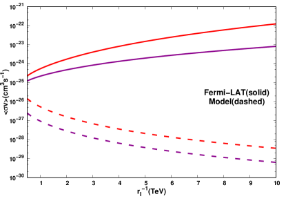
Figure 3: Thermal-averaged cross sections (dashed lines) for $B_{\mu}^{(0,1)}B_{\mu}^{(0,1)}\to W^{+}W^{-}$ (blue) and $B_{\mu}^{(0,1)}B_{\mu}^{(0,1)}\to\tau^{+}\tau^{-}$ (red) as a function of the DM mass for $\Lambda=3\,{\rm max}(R_{q}^{-1},r_{\ell}^{-1})$. Also shown are the median upper limits on the DM annihilation cross-section as derived from a combined analysis of the Fermi-LAT data Ackermann:2015zua .

6 LHC Signatures

In the preceding section, we saw that this model admits much heavier DM candidates (consistent with the relic abundance) than allowed within the minimal-UED paradigm (whether 5– or 6–dimensional). It now behoves us to examine the collider phenomenology of the same. Naively, a constriction of the moduli $(r_{\ell},R_{q})$ that this model allows for would render the fields heavier, thereby suppressing the production rates and easing the collider bounds as compared to UED-like scenarios. On the other hand, the very structure of the theory, namely that only one of the possibly two $Z_{2}$ parities is conserved, brings forth new modes, both in the production arena as well as in decays. To this end, we begin by reminding ourselves of some the particularly interesting couplings.

• Although $Z_{2}^{(q)}$ is not an exact symmetry, with the quark and gluon fields being confined to the 4-branes at $x_{5}=0,\pi$, this symmetry is effectively an exact one in the context of the strong interactions. Thus, the first KK-state of the quarks ($q^{(1,0)}$) and gluons ($g^{(1,0)}$) can, essentially, be produced only in pairs. The latter, being heavier, would decay predominantly into $q^{(1,0)}+\bar{q}^{(0,0)}$ pairs. The $q^{(1,0)}$, on the other hand, would decay into a SM-quark and the $B_{\mu}^{(1,0)}$ or a $W_{\mu}^{a\,(1,0)}$ with the branching fraction depending on the quark chirality. The bosons, in turn, would decay into leptons.

  The final state, from such production and decay channels, would, typically, comprise of (mostly soft) jets and charged leptons (or missing transverse momentum on account of neutrinos). The latter (MET) would be similar to the classic mUED signal and, hence, subject our model to the same constraints. For a mass of the parent particle similar to the mUED case, however, the fraction of events with a similar quantum of MET would be significantly smaller. While this suppression would be compensated by the presence of events with charged leptons, it is clear that the ensuing constraints would be similar to those applicable to the mUED case. Thus, a simple increase of the scale ($R_{q}^{-1}\mathrel{\hbox to0.0pt{\raise 2.15277pt\hbox{$>$}\hss}{\lower 2.15277pt\hbox{$\sim$}}}2\,{\rm TeV}$) would maintain consistency with non-observation at the LHC.

• An interesting alternative would be the resonant production $pp\to g^{(2,0)}+X$ starting with a $q\bar{q}$ pair (or, the analogous $q+g\to q^{(2,0)}$). Either of these vertices are loop-suppressed, leading to small cross sections. Once again, $g^{(2,0)}\to q^{(1,0)}+\bar{q}^{(1,0)}$ with the subsequent cascades as in the preceding cases. The signal too is similar, but of a markedly smaller size. It might seem that a invariant mass reconstruction (possible, in principle, for the $4\ell+$ soft jets final state) would increase the signal significance. Given the smallness of the signal cross section, and the softness of the jets (leading to potential confusion with other sources such as pileups and multiple collisions), this is quite unlikely. A more definitive statement would require a full simulation beyond the scope of this paper.

• More interestingly, a SM $\bar{q}\,q^{(^{\prime})}$ pair has unsuppressed couplings with each of $B_{\mu}^{(0,2)}$ and $W_{\mu}^{a\,(0,2)}$. The latter, though, have only loop-suppressed couplings with a pair of SM leptons. Thus, for $r_{l}^{-1}<R_{q}^{-1}$, the charged gauge bosons would manifest themselves as a leptophobic $W^{\prime}$ while the two neutral ones would act like (nearly degenerate) pair of leptophobic $Z^{\prime}$s.

  The CMS collaboration has studied dijet final states in the quest for such resonances and the absence of any anomalies has led to constraints of the form $m_{W^{\prime}}>2.7\,{\rm TeV}$ and $m_{Z^{\prime}}>2.1\,{\rm TeV}$ Sirunyan:2016iap . It should be noted that the inclusion of all the four electroweak $(0,2)$ KK-states would translate to a stronger bound. Furthermore, the aforementioned limits were obtained from the analysis of only $12.9\,{\rm fb}^{-1}$ of data and assuming that no such anomaly would show up in the current round would push the bound up considerably. Thus, it might be safely assumed that $r_{\ell}^{-1}\mathrel{\hbox to0.0pt{\raise 2.15277pt\hbox{$<$}\hss}{\lower 2.15277pt\hbox{$\sim$}}}1.7\,{\rm TeV}$ would be strongly disfavored.

• For $r_{\ell}^{-1}>R_{q}^{-1}$, on the other hand, the situation is altered quite dramatically. The $B_{\mu}^{(0,2)}$ and $W_{\mu}^{a\,(0,2)}$ can, now, decay to the first KK excitations of the quarks as well. The branching ratio into SM quarks decreases while that into the first KK quark states increases as $r_{l}^{-1}$ becomes progressively greater than $R_{q}^{-1}$. Furthermore, note that the coupling of the $B_{\mu}^{(0,2)}$ to the singlet up-type quarks is larger than those to the other quarks. These features are reflected in the plots as presented in Fig. 4.

  The level-1 quarks would further decay into a SM quark and a $B_{\mu}^{(1,0)}$ or $W_{\mu}^{a\,(1,0)}$, with the latter cascading down to leptons. In the final analysis, such a chain would result in a final state comprised of soft jets and leptons. This signal is, understandably, more difficult to analyze (as compared to the dijet signal discussed in the previous instant) but can still act as a complementary signal.

• There are various studies Burdman:2006gy ; Choudhury:2011jk ; Burdman:2016njl on the collider phenomenology of 6D models like $T_{2}/Z_{2}$ or $T_{2}/Z_{4}$. However, the findings of the aforementioned studies cannot be directly translated to our case. With the mass spectrum and couplings in the older models (studied there) being very different from the model under consideration, most of the signals and strategies suggested in the earlier analyses are not applicable here. The major difference is due to the fact that $Z_{2}^{(q)}$ is not an exact symmetry. As a result, the second KK level gauge bosons (along quark brane) and quarks decay to SM leptons at tree level in contrast to the cases considered in Refs.Burdman:2006gy ; Choudhury:2011jk ; Burdman:2016njl where the corresponding decays only occur at the loop level.

  For very similar reasons, even recent studies Choudhury:2016tff ; Deutschmann:2017bth ; Beuria:2017jez that seek to use experimental analyses in multiple channels (multijets, or dileptons with jets, each accompanied by missing transverse energy) also fail to apply. Rather, one needs to consider the event topologies described above.

• As we shall see in the next section, low energy constraints, unless tamed by the introduction of compensatory fields, tend to push up $R_{q}^{-1}$ and, hence, the quark and gluon resonances to levels that are not easily accessible at the LHC. One would, then, have to concentrate on the KK-excitations of the leptons and electroweak bosons, and, consequently, devise algorithms more sensitive than those that have been deployed so far.

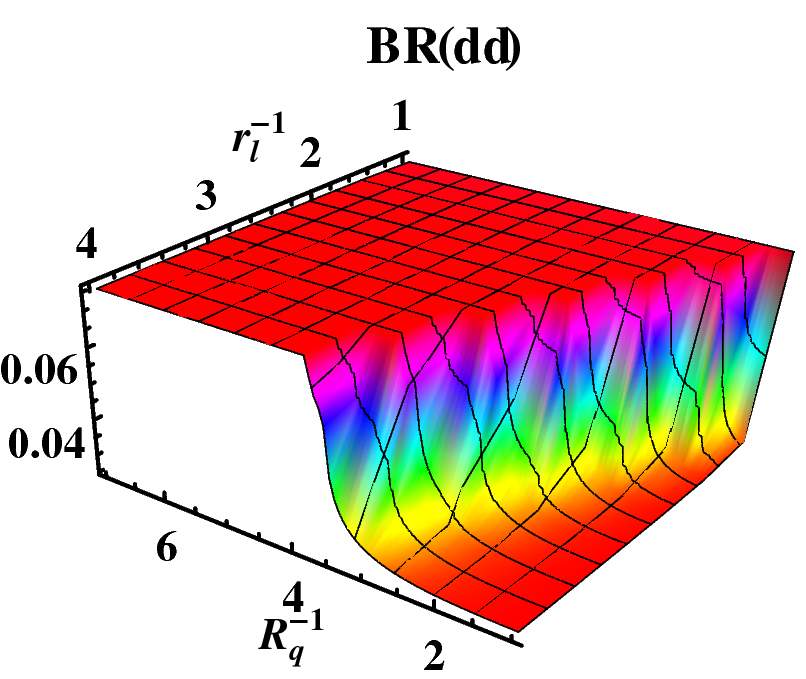
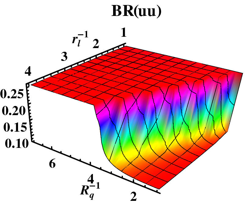
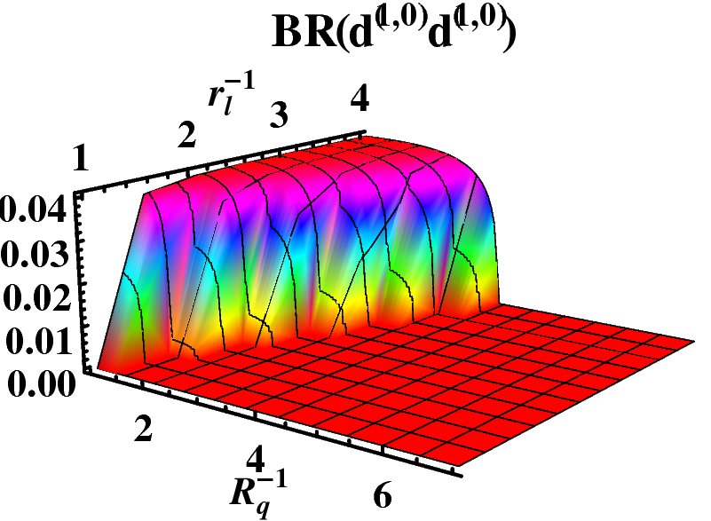
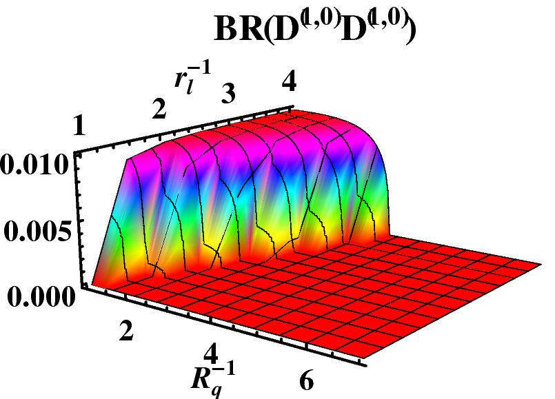
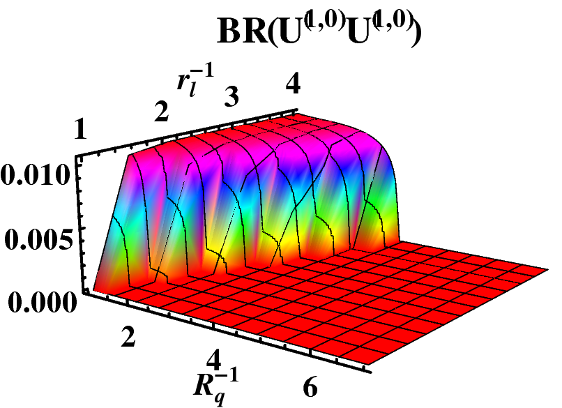
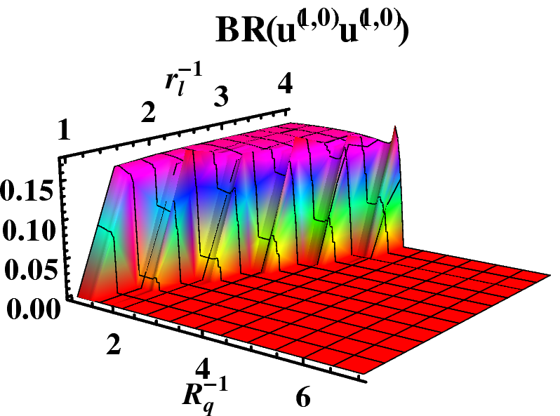
Figure 4: Branching ratios of $B^{(0,2)}$ for down-type(d) and up-type quarks(u) as the final states. The quark singlets and doublets are represented by $d$ and $D$ respectively. $\Lambda R=20$ has been assumed in the calculation.

7 Low energy constraints

Stronger constraints emanate from low-energy physics, in particular, the observables precisely measured at LEP and the SLD.

7.1 Effective four fermi interaction

An important consequence of the fermions being brane-localized, while the gauge bosons traverse the bulk, is that KK-number violating gauge-fermion couplings appear. Their presence immediately results in the alteration of the effective four-fermion interactions at low-energies, the strength for which is usually parametrized in terms of $G_{f}$.

In the present case, there exists a further subtlety. For the SM leptons, only the $W^{a,\,(n,0)}$ and the $B^{a,\,(n,0)}$ contribute at the tree level. For the quarks, on the other hand, the $Z_{2}$ symmetry ensures that the odd modes do not, and only the $W^{a,\,(0,2n)}$ and the $B^{a,\,(0,2n)}$ contribute. Furthermore, none of these KK-excitations couple to both quarks and leptons.

The best measurement of $G_{f}$ is given by $G_{\mu}$, the effective coupling strength for the muon decay. In the present case, this gets modified to

$$\begin{array}[]{rcl}G_{\mu}&=&\displaystyle G_{\mu}^{(SM)}\left[1+\sum_{n>0}\left(\frac{g^{(n,0)}m_{W}}{g\,m_{W^{(n,0)}}}\right)^{2}\right]\\ &\equiv&G_{\mu}^{(SM)}\,(1+V).\end{array}$$ (27)

Using, $g^{(n,0)}=\sqrt{2}\,g$ and simplifying the sum by neglecting the electroweak contribution to the masses in comparison to the KK-contribution, namely

$$\sum_{n>0}\frac{1}{m_{W^{(n,0)}}^{2}}\mathrel{\hbox to0.0pt{\raise 2.15277pt\hbox{$>$}\hss}{\lower 2.15277pt\hbox{$\sim$}}}R_{q}^{2}\,\sum_{n>0}\frac{1}{n^{2}}$$

we have

$$V\approx 2\,\zeta(2)\,m_{W}^{2}\,R_{q}^{2}.$$

Electroweak precision data constrains $V\leq 0.0013$ implying $R_{q}^{-1}\mathrel{\hbox to0.0pt{\raise 2.15277pt\hbox{$<$}\hss}{\lower 2.15277pt\hbox{$\sim$}}}4\,{\rm TeV}$.

Had the four-quark effective operator been measured as accurately as $G_{\mu}$, we would have been led to a bound on $r_{\ell}^{-1}$ that is a factor of 2 weaker. However, low energy data on this is not as precise, with the inaccuracy exacerbated by the lack of a full understanding of bound-state effects in hadrons. Consequently, the corresponding bounds are actually much weaker and of little relevance to us.

7.2 Oblique Variables

We present here the one-loop contributions to the electroweak precision observables. We adopt the parametrization due to Ref.Peskin:1991sw , and omit the third parameter ($U$) as it is of little relevance in the present case. The definitions, in terms of the self-energies, are

$$\begin{array}[]{rcl}\displaystyle\frac{\alpha}{4s_{w}^{2}\,c_{w}^{2}}\,S&=&\displaystyle\frac{\Pi_{ZZ}(m_{Z}^{2})-\Pi_{ZZ}(0)}{m_{Z}^{2}}-\left.\frac{\partial\Pi_{\gamma\gamma}(p^{2})}{\partial p^{2}}\right|_{p^{2}=0}-\frac{c_{w}^{2}-s_{w}^{2}}{c_{w}\,s_{w}}\left.\frac{\partial\Pi_{\gamma\,Z}(p^{2})}{\partial p^{2}}\right|_{p^{2}=0}\\[8.61108pt] \alpha\,T&=&\displaystyle\frac{\Pi_{WW}(0)}{m_{W}^{2}}-\frac{\Pi_{ZZ}(0)}{m_{Z}^{2}}-2c_{w}\,s_{w}\frac{\Pi_{Z\gamma}(0)}{m_{W}^{2}}\end{array}$$ (28)

Since the SM contributions are well known, we consider here only the deviations from the SM values, namely,

$$\mathcal{S}\equiv S-S_{SM}\ ,\qquad\mathcal{T}\equiv T-T_{SM}\ .$$ (29)

In calculating the loops, we neglect further small corrections (wherever applicable) wrought by the changes in the wavefunctions. While the observables ${\cal S,T}$ are finite (and, independent of the renormalization scale), the individual loops are divergent and are calculated using dimensional regularization. Using the expressions derived in the Appendix, we list below the individual contributions wrought by the various fields:

• Fermions
  On account of the large Yukawa coupling, the contributions due to the top-partners far outweigh the rest and we have, for an individual excitation of mass $m_{n}$,

  $$\mathcal{S}\approx\frac{m_{t}^{2}}{12\pi\,m_{n}^{2}}\ ,\qquad\mathcal{T}\approx\frac{m_{t}^{4}}{8\,\pi\,s_{w}^{2}\,m_{n}^{2}\,m_{W}^{2}}.$$ (30)

• Gauge bosons
  These contributions are very small, in particular to ${\cal S}$. For the $(n,0)$ and $(0,n)$ states, we have the individual contributions to be

  $$\mathcal{S}\approx\frac{3m_{Z}^{2}s_{w}^{4}}{5\pi\,m_{n}^{2}}\ ,\qquad\mathcal{T}\approx\frac{m_{W}^{2}}{\pi\,c_{w}^{2}\,m_{n}^{2}}\ ,$$ (31)

  whereas for the excitations with non-zero KK-numbers in both directions, an additional factor of 1/2 appears for both ${\cal S,T}$.

• Higgs bosons
  If the Higgs is corner-located, there are no additional loops and the only additional contribution accrues from the changes in the wavefunctions. For the 4-brane localized Higgs, on the other hand, there is a single tower of scalars to be considered, in addition to contributions from the changes in the gauge-boson wavefunctions as alluded to in Sec.. And, finally, for bulk higgs, corrections accrue only from the tower of towers (of scalars). The loop corrections, for $(n,0)$ and $(0,n)$ Higgs bosons, are

  $$\mathcal{S}\approx\frac{m_{h}^{2}-3m_{Z}^{2}}{12\pi m_{n}^{2}}\ ,\qquad\mathcal{T}\approx-\,\frac{5m_{H}^{2}}{24\,\pi\,c_{w}^{2}\,m_{n}^{2}}-\,\frac{7\,m_{W}^{2}}{24\,\pi\,c_{w}^{2}m_{n}^{2}}$$ (32)

  whereas for those with non-zero KK-numbers in both directions, an additional factor of 1/2 appears as in the gauge boson case.

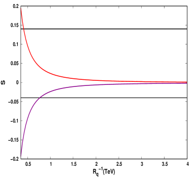
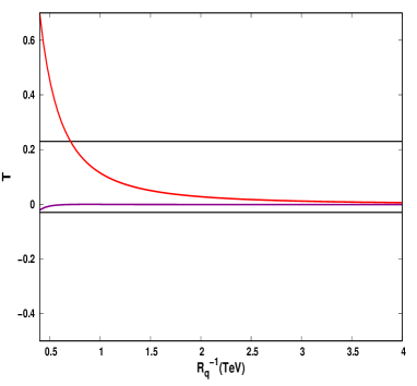
Figure 5: ${\cal S}$ vs $R_{q}^{-1}$ and ${\cal T}$ vs $R_{q}^{-1}$ obtained using $c_{1,2}=1$(red) and $c_{1,2}=-1$(blue). The horizontal bands correspond to the 95% C.L experimental constraints.

The individual contributions have, of course, to be summed over the respective towers, and herein lies a problem. For a single tower, the sum is a finite one. Exactly as in the preceding section, in the limit of a vanishing electroweak scale—as compared to the compactification scale—this can be expressed in terms of $\zeta(2)$.

Neglecting, for the time being, the six-dimensional nature of the bosonic fields, the contribution from the top sector far overwhelms the others. (Indeed, in this approximation, the contribution due to Higgs and gauge bosons to T parameter is 5%.). Consequently, the ${\cal S,T}$ parameters are expected to primarily constrain $R_{q}^{-1}$, with only minor sensitivity to $r_{\ell}^{-1}$.

However, for a tower of towers (as is the case for a six dimensional field), the sum is logarithmically divergent. Though the sensitivity to the cut off is only a logarithmic one, we still cannot expect a reliable estimate for the $S$ and $T$ parameters by only summing the KK modes. The physics above cut-off ($\Lambda$) of the theory is relevant, and the corresponding contribution to the parameters can be roughly estimated using higher dimension custodial symmetry breaking operators as discussed in Ref.Appelquist:2002wb , leading to

$$\begin{array}[]{rcl}T^{\text{UV}}&=&\displaystyle c_{1}\frac{m_{H}^{2}}{4\Lambda^{2}\alpha(m_{Z})}\\ S^{\text{UV}}&=&\displaystyle c_{2}\frac{2\pi v^{2}}{\Lambda^{2}}\end{array}$$ (33)

Here, $c_{1,2}$ are constants giving the extent of custodial symmetry breaking and deviation of coupling of $W^{3}$ and hypercharge $B$ gauge field from the SM case respectively. Assuming maximal custodial symmetry violation, we consider both $c_{1,2}=\pm 1$.

The values of $T^{\text{UV}}$ and $S^{\text{UV}}$ are dependent only on the cut-off, which, in turn, is dependent on the number of dimensions. As we have noted earlier, the stability of the electroweak vacuum as well considerations of the naturalness of Higgs mass Appelquist:2002wb ; Appelquist:2000nn indicates that the maximal cutoff is $\Lambda=3\,R^{-1}$. This is the value of $\Lambda$ we assume in producing Fig.5. This, in turn, implies that in calculating the loop contributions, only fields with masses less than $\Lambda$ are to be included. Interestingly, for the chosen values of $|c_{1,2}|=1$, the contribution of the operators of eqn(33) to the ${\cal T}$-parameter is equal to that of loop corrections due to quarks while in case of ${\cal S}$, it is entirely dominating.

As can be gleaned from Fig.5, the constraints from the electroweak precision variables, resulting from the experimental measurements Baak:2014ora , which for ${\cal U}=0$, read

$${\cal S}=0.05\pm 0.09\ ,\qquad{\cal T}=0.1\pm 0.13\qquad\mbox{(errors at 95\% C.L.)},$$

are very weak indeed. Evidently, they pale in comparison to the restrictions imposed by the other observables.

8 Summary

Non-observation of any new state at the LHC has severely constrained the parameter space for a host of well-motivated theories going beyond the SM. In particular, the minimal UED suffers from the problem that this non-observation militates strongly against the upper limit on the compactification scale dictated by the observed DM relic density. The ensuing tension can be relieved, to an extent, by invoking a non-minimal theory with boundary-localized terms (respecting a $Z_{2}$ symmetry so that an explanation for the DM can be retained). However, the continuing absence of any signals requires the size of such terms (ostensibly, the result of quantum corrections) to become ever larger, thereby severely straining the entire paradigm.

To mitigate the problems faced by the minimal UED, in this work, we considered a quasi-universal six-dimensional theory, which naturally inherits a much richer phenomenology compared to its five-dimensional (or, even, usual six-dimensional) counterpart. Apart from the interesting double-tower signatures, this scenario brings in many more manifestations of possible BSM scenarios, due to the distinctively different orbifolding of the space and field-localizations.

The scenario is quasi-universal in the sense that the quarks (and gluons) and leptons are localized on orthogonal branes, while only the electroweak gauge bosons traverse the entire bulk. This decouples the masses of the quark and leptonic towers (by allowing for different compactification radii), thereby enabling one to maintain the putative DM at a suitably low mass, while rendering the quark and gluon excitations relatively inaccessible at the LHC.

Naively duplicating the canonical mUED structure, however, is not phenomenologically viable as this would have left behind a pair of $Z_{2}$-symmetries, thereby leaving behind three DM fields, one each for the lightest excitations in the $(1,0)$, $(0,1)$ and $(1,1)$ sectors. Two of these masses would be determined by the quark-excitation scale and would run foul of the relic density measurements.

To this end, we propose that the quarks (and gluons) are localized on a pair of parallel end-of-the-world 4-branes, while the leptonic fields are localized on a single such brane orthogonal to the other two. The electroweak gauge bosons must, obviously, extend across the entire bulk. For the Higgs, several alternatives are possibles, such as localizing them to the corners of the brane-box, allowing them to be localized on the boundary-branes or to propagate in the entire bulk. Localization, whether at corners or on branes, leads to boundary localized mass terms that can significantly modify the gauge boson wavefunction and their coupling with SM fermions. Thus the simplest alternative, devoid of such issues, is to allow the Higgs field to traverse the entire bulk.

The hard breaking of one of the two $Z_{2}$’s engenders unsuppressed tree-level couplings, amongst others, for certain level-1 KK-excitations with a pair of SM fields. This not only renders two of the putative DM candidates unstable (leaving behind the $B_{\mu}^{(0,1)}$ as the only cosmologically stable particle), but also has immense consequences as far as LHC signals are concerned. The prompt decay of all the excitations along the quark-direction into SM particles severely depletes the missing transverse momentum signal, a cornerstone of LHC search strategies. Instead, they are manifested in terms of a dijet final state, or final states with leptons and soft jets. As of the present instant, it is the former modes that present the strongest constraints, with the negative searches for leptophobic $W^{\prime}/Z^{\prime}$, together, requiring that a DM mass $\mathrel{\hbox to0.0pt{\raise 2.15277pt\hbox{$<$}\hss}{\lower 2.15277pt\hbox{$\sim$}}}1.7\,{\rm TeV}$ would be strongly disfavored. However, even stronger bounds are imposed by low energy experiments. The KK number violating $W^{a(n,0)}\bar{\ell}{\ell}$ couplings modify the effective four-lepton interactions at low energies and the high-precision measurement of $G_{\mu}$ imposes a constraint $R_{q}^{-1}\mathrel{\hbox to0.0pt{\raise 2.15277pt\hbox{$<$}\hss}{\lower 2.15277pt\hbox{$\sim$}}}4\,{\rm TeV}$. It should be realized, though, this bound is strictly applicable only when the contribution of the infinite tower is included. For any such theory with a finite cutoff (as it must have), the bound weakens to an appreciable degree. The corresponding bounds on $r_{\ell}^{-1}$ are weaker by more than a factor of 2, not only on account of hadronic uncertainties, but also because only half as many $W^{a(0,n)}$s (namely, the even modes alone) mediate the four-quark interaction term. The bounds from electroweak precision variables ${\cal S}$ and ${\cal T}$ are much weaker in comparison to that from the measurement of $G_{\mu}$.

Even the (weaker) LHC bound is stronger than that imposed, by considerations of the relic density, on the mUED candidate for the DM. In other words, this seems to bely our stated objective of easing the twin-constraints (LHC and DM). However, the aforementioned breaking of one of the $Z_{2}$’s manifests in a nontrivial way in the determination of the number densities. With the quark-direction excitations of the electroweak gauge bosons now having unsuppressed couplings with all the SM fermions, as well as their own (unidirectional) excitations, these can mediate interactions between the SM particles and the first excited states of the leptons (which are close to the DM in mass). As a consequence, these leptonic states remain in equilibrium until a later epoch, thereby suppressing their density at decoupling. This, in turn, translates to their decays—into the SM leptons and the DM—no longer being effective means to replenish the relic density. Since this replenishment is actually the major contributor to the relic density in UED-like scenarios, this effect can suppress $\Omega_{\rm DM}$ to levels well below the observed one, especially for $2\,r_{\ell}^{-1}\sim n\,R_{q}^{-1}\,(n\in\mathbb{Z}^{+})$, namely regions of parameter space where the aforementioned $s$-channel processes are relatively close to being on resonance.

This curious effect has profound implications, with multi-TeV DM being quite in consonance with all bounds (relic density, dedicated direct and indirect searches as well as the LHC constraints), without any fine tuning being necessary. In addition, this scenario promises very interesting signals at colliders (both in the forthcoming runs of the LHC as well as in future high-energy $e^{+}e^{-}$ colliders). It is, thus, worthwhile, to consider such scenarios very seriously and subject them to rigorous tests, both in the context of colliders as well as low-energy constraints, especially those pertaining to flavour. We plan to examine real issues in future publication.

Appendix A Appendix : One loop contributions to gauge boson self energies

In calculating the loop-contributions of the KK-particles to $\mathcal{S,T}$, we consider only the leading terms and neglect effects due to the deformations of the wavefunctions. It is useful, in this context to define the function

$$f(m_{n},m_{1},m_{2})=\log\frac{m_{n}^{2}-x(1-x)p^{2}+(1-x)m_{1}^{2}+x\,m_{2}^{2}}{\mu^{2}}$$ (34)

where the dependence of $f$ on the momentum $p$ and the renormalization scale $\mu$ has been suppressed. The dependence of the measurables $\mathcal{S,T}$ on $\mu$ actually vanishes, as it should.

We, now, list the various loop-contributions to the self-energies in question. We use dimensional regularization, working in $4-\epsilon$ dimensions and define

$${\cal A}\equiv\frac{2}{\epsilon}\,-\gamma_{E}+\log(4\pi)$$ (35)

where $\gamma_{E}$ is the Euler-Mascheroni constant.

Contribution of KK quarks

Numerically, only the contribution due to the top-partners are of any importance and these are given by

$$\begin{array}[]{rcl}\Pi^{Q}_{\gamma\gamma}(p^{2})&=&\displaystyle\frac{\alpha}{4\pi}\frac{-8}{3}\int^{1}_{0}dx\,\left[\frac{5}{3}{\cal A}-2x(1-x)p^{2}\,\left(4f(m_{n},m_{t},m_{t})+f(m_{n},0,0)\right)\right]\\[8.61108pt] \Pi^{Q}_{ZZ}(p^{2})&=&\displaystyle\frac{\alpha}{4\pi}\,\frac{-3+8s_{w}^{2}-\frac{32}{3}s_{w}^{4}}{s_{w}^{2}c_{w}^{2}}\,(2\,p^{2})\,\int^{1}_{0}dx\,x(1-x)\,\left({\cal A}-f(m_{n},m_{t},m_{t})\right)\\[4.30554pt] &+&\displaystyle\frac{\alpha}{4\pi}\,\frac{3}{s_{w}^{2}c_{w}^{2}}\,\int^{1}_{0}dx\,\left({\cal A}-f(m_{n},m_{t},m_{t})\right)m_{t}^{2}\\[4.30554pt] &+&\displaystyle\frac{\alpha}{4\pi}\,\frac{-3+4s_{w}^{2}-\frac{8}{3}s_{w}^{4}}{s_{w}^{2}c_{w}^{2}}\,(2\,p^{2})\,\int^{1}_{0}dx\,x(1-x)\,\left({\cal A}-f(m_{n},0,0)\right)\\[8.61108pt] \Pi^{Q}_{Z\gamma}(p^{2})&=&\displaystyle\frac{\alpha}{4\pi}\,\frac{-4+\frac{32}{3}s_{w}^{2}}{s_{w}c_{w}}\,(2\,p^{2})\,\int^{1}_{0}dx\,x(1-x)\,\left({\cal A}-f(m_{n},m_{t},m_{t})\right)\\[4.30554pt] &+&\displaystyle\frac{\alpha}{4\pi}\,\frac{-2+\frac{8}{3}s_{w}^{2}}{s_{w}c_{w}}\,(2\,p^{2})\,\int^{1}_{0}dx\,x(1-x)\,\left({\cal A}-f(m_{n},0,0)\right)\\[8.61108pt] \Pi^{Q}_{WW}(p^{2})&=&\displaystyle\frac{\alpha}{4\pi}\,\frac{-6}{s_{w}^{2}}\,\int^{1}_{0}dx\,\left({\cal A}-f(m_{n},m_{b},m_{t})\right)\left(2x(1-x)p^{2}-x\,m_{t}^{2}-(1-x)\,m_{b}^{2}\right)\\ \end{array}$$ (36)

Contribution of KK Gauge bosons and Ghosts

We sum here the contributions of the gauge bosons and ghosts of a given KK order. Further, we neglect the small splitting between the various fields at a given level emanating from electroweak symmetry breaking. Remembering that the KK-idex, $n$ now has two components, we have

$$\begin{array}[]{rcl}\Pi^{GB}_{\gamma\gamma}(p^{2})&=&\displaystyle\frac{\alpha}{4\pi}\displaystyle\int^{1}_{0}dx\,\left({\cal A}-f(m_{n},m_{W},m_{W})\right)\,\left((-12x^{2}+20x-3)p^{2}+2m_{W}^{2}\right)\\[8.61108pt] \Pi^{GB}_{ZZ}(p^{2})&=&\displaystyle\frac{\alpha}{4\pi}\,\frac{c_{w}^{2}}{s_{w}^{2}}\,\int^{1}_{0}dx\,\left({\cal A}-f(m_{n},m_{W},m_{W})\right)\,\left((-12x^{2}+20x-3)p^{2}+2m_{W}^{2}\right)\\[8.61108pt] \Pi^{GB}_{\gamma Z}(p^{2})&=&\displaystyle\frac{\alpha}{4\pi}\,\frac{c_{w}}{s_{w}}\,\int^{1}_{0}dx\,\left({\cal A}-f(m_{n},m_{W},m_{W})\right)\,\left((-12x^{2}+20x-3)p^{2}+2m_{W}^{2}\right)\\[8.61108pt] \Pi^{GB}_{WW}(p^{2})&=&\displaystyle\frac{\alpha}{4\pi}\,\frac{c_{w}^{2}}{s_{w}^{2}}\,\int^{1}_{0}dx\,\left({\cal A}-f(m_{n},m_{W},m_{Z})\right)\\ &&\displaystyle\hskip 80.00012pt\left[(-12x^{2}+12x+1)p^{2}+2(2-3x)m_{Z}^{2}+2(3x-1)m_{W}^{2}\right]\\[4.30554pt] &+&\displaystyle\frac{\alpha}{4\pi}\int^{1}_{0}dx\,\left({\cal A}-f(m_{n},m_{W},0)\right)\,\left[(-12x^{2}+12x+1)p^{2}+2(3x-1)m_{W}^{2}\right]\end{array}$$ (37)

Contribution of KK Higgs bosons

For the case of Higgs bosons defined on the 4-branes at $x_{4}=0,\pi$, we have

$$\begin{array}[]{rcl}\Pi^{H}_{\gamma\gamma}(p^{2})&=&\displaystyle\frac{\alpha}{4\pi}\,\int^{1}_{0}dx\,\left({\cal A}-f(m_{n},m_{W},m_{W})\right)\,\left((-4x^{2}+6x-2)p^{2}-2m_{W}^{2}\right)\\[8.61108pt] \Pi^{H}_{\gamma Z}(p^{2})&=&\displaystyle\frac{\alpha}{4\pi}\,\frac{s_{w}}{c_{w}}\,\int^{1}_{0}dx\,\left({\cal A}-f(m_{n},m_{W},m_{W})\right)\,\left((2x^{2}-3x+1)p^{2}+2m_{W}^{2}\right)\\[8.61108pt] &+&\displaystyle\frac{\alpha}{4\pi}\,\frac{c_{w}}{s_{w}}\,\int^{1}_{0}dx\,\left({\cal A}-f(m_{n},m_{W},m_{W})\right)\,\left((-2x^{2}+3x-1)p^{2}\right)\\[8.61108pt] \Pi^{H}_{ZZ}(p^{2})&=&\displaystyle\frac{\alpha}{4\pi}\,\frac{1}{4\,c_{w}^{2}\,s_{w}^{2}}\,\int^{1}_{0}dx\,\left({\cal A}-f(m_{n},m_{Z},m_{H})\right)\\ &&\displaystyle\hskip 80.00012pt\left[(-4x^{2}+4x-1)p^{2}+(1-2x)m_{H}^{2}+(2x-5)m_{Z}^{2}\right]\\[8.61108pt] &+&\displaystyle\frac{\alpha}{4\pi}\,\frac{c_{2w}^{2}}{2\,s_{w}\,c_{w}}\,p^{2}\,\int^{1}_{0}dx\,\left({\cal A}-f(m_{n},m_{W},m_{W})\right)\,(-2x^{2}+3x-1)\\[4.30554pt] &-&\displaystyle\frac{\alpha}{2\pi}s_{w}^{2}\,m_{Z}^{2}\,\int^{1}_{0}dx\,\left({\cal A}-f(m_{n},m_{W},m_{W})\right)\\[8.61108pt] \Pi^{H}_{WW}(p^{2})&=&\displaystyle\frac{\alpha}{4\pi}\,\frac{1}{4s_{w}^{2}}\,\int^{1}_{0}dx\,\left({\cal A}-f(m_{n},m_{W},m_{Z})\right)\\ &&\displaystyle\hskip 80.00012pt\left[((4x-4x^{2}-1)p^{2}+(1-2x)m_{Z}^{2}+(2x-1)m_{W}^{2}\right]\\[4.30554pt] &-&\displaystyle\frac{\alpha\,s_{w}^{2}}{4\pi}\,\int^{1}_{0}dx\,\left({\cal A}-f(m_{n},m_{W},m_{Z})\right)\,m_{Z}^{2}\\[4.30554pt] &-&\frac{\alpha}{4\pi}\,\int^{1}_{0}dx\,\left({\cal A}-f(m_{n},m_{W},m_{H})\right)\\ &&\displaystyle\hskip 80.00012pt\left[(4x-4x^{2}-1)p^{2}+(2x-5)m_{W}^{2}+(1-2x)m_{H}^{2}\right]\end{array}$$ (38)

References

- (1) ATLAS collaboration, G. Aad et al., Observation of a new particle in the search for the Standard Model Higgs boson with the ATLAS detector at the LHC, Phys. Lett. B716 (2012) 1–29, [1207.7214].
- (2) ATLAS collaboration, G. Aad et al., Combined search for the Standard Model Higgs boson in collisions at TeV with the ATLAS detector, Phys. Rev. D86 (2012) 032003, [1207.0319].
- (3) CMS collaboration, S. Chatrchyan et al., Observation of a new boson at a mass of 125 GeV with the CMS experiment at the LHC, Phys. Lett. B716 (2012) 30–61, [1207.7235].
- (4) H.-C. Cheng, K. T. Matchev and M. Schmaltz, Radiative corrections to Kaluza-Klein masses, Phys. Rev. D66 (2002) 036005, [hep-ph/0204342].
- (5) G. Servant and T. M. P. Tait, Is the lightest Kaluza-Klein particle a viable dark matter candidate?, Nucl. Phys. B650 (2003) 391–419, [hep-ph/0206071].
- (6) K. Kong and K. T. Matchev, Precise calculation of the relic density of Kaluza-Klein dark matter in universal extra dimensions, JHEP 01 (2006) 038, [hep-ph/0509119].
- (7) F. Burnell and G. D. Kribs, The Abundance of Kaluza-Klein dark matter with coannihilation, Phys. Rev. D73 (2006) 015001, [hep-ph/0509118].
- (8) M. Kakizaki, S. Matsumoto and M. Senami, Relic abundance of dark matter in the minimal universal extra dimension model, Phys. Rev. D74 (2006) 023504, [hep-ph/0605280].
- (9) G. Belanger, M. Kakizaki and A. Pukhov, Dark matter in UED: The Role of the second KK level, JCAP 1102 (2011) 009, [1012.2577].
- (10) M. Baak, M. Goebel, J. Haller, A. Hoecker, D. Ludwig, K. Moenig et al., Updated Status of the Global Electroweak Fit and Constraints on New Physics, Eur. Phys. J. C72 (2012) 2003, [1107.0975].
- (11) U. Haisch and A. Weiler, Bound on minimal universal extra dimensions from anti-B —> X(s)gamma, Phys. Rev. D76 (2007) 034014, [hep-ph/0703064].
- (12) U. K. Dey and T. Jha, Rare top decays in minimal and nonminimal universal extra dimension models, Phys. Rev. D94 (2016) 056011, [1602.03286].
- (13) D. Choudhury and K. Ghosh, Bounds on Universal Extra Dimension from LHC Run I and II data, Phys. Lett. B763 (2016) 155–160, [1606.04084].
- (14) N. Deutschmann, T. Flacke and J. S. Kim, Current LHC Constraints on Minimal Universal Extra Dimensions, Phys. Lett. B771 (2017) 515–520, [1702.00410].
- (15) J. Beuria, A. Datta, D. Debnath and K. T. Matchev, LHC Collider Phenomenology of Minimal Universal Extra Dimensions, 1702.00413.
- (16) ATLAS collaboration, T. A. collaboration, Search for direct top squark pair production and dark matter production in final states with two leptons in TeV collisions using 13.3 fb-1 of ATLAS data, .
- (17) ATLAS collaboration, T. A. collaboration, Search for squarks and gluinos in events with an isolated lepton, jets and missing transverse momentum at = 13 TeV with the ATLAS detector, .
- (18) WMAP collaboration, E. Komatsu et al., Seven-Year Wilkinson Microwave Anisotropy Probe (WMAP) Observations: Cosmological Interpretation, Astrophys. J. Suppl. 192 (2011) 18, [1001.4538].
- (19) Planck collaboration, P. A. R. Ade et al., Planck 2015 results. XIII. Cosmological parameters, Astron. Astrophys. 594 (2016) A13, [1502.01589].
- (20) G. Burdman, B. A. Dobrescu and E. Ponton, Six-dimensional gauge theory on the chiral square, JHEP 02 (2006) 033, [hep-ph/0506334].
- (21) B. A. Dobrescu and E. Ponton, Chiral compactification on a square, JHEP 03 (2004) 071, [hep-th/0401032].
- (22) N. Maru, T. Nomura, J. Sato and M. Yamanaka, The Universal Extra Dimensional Model with S**2/Z(2) extra-space, Nucl. Phys. B830 (2010) 414–433, [0904.1909].
- (23) G. Cacciapaglia, A. Deandrea and J. Llodra-Perez, A Dark Matter candidate from Lorentz Invariance in 6D, JHEP 03 (2010) 083, [0907.4993].
- (24) H. Dohi and K.-y. Oda, Universal Extra Dimensions on Real Projective Plane, Phys. Lett. B692 (2010) 114–120, [1004.3722].
- (25) B. A. Dobrescu, D. Hooper, K. Kong and R. Mahbubani, Spinless photon dark matter from two universal extra dimensions, JCAP 0710 (2007) 012, [0706.3409].
- (26) M. T. Arun and D. Choudhury, Stabilization of moduli in spacetime with nested warping and the UED, Nucl. Phys. B923 (2017) 258–276, [1606.00642].
- (27) M. T. Arun, D. Choudhury and D. Sachdeva, Universal Extra Dimensions and the Graviton Portal to Dark Matter, JCAP 1710 (2017) 041, [1703.04985].
- (28) T.-j. Li, GUT breaking on M**4 x T**2 / (Z(2) x Z-prime (2)), Phys. Lett. B520 (2001) 377–384, [hep-th/0107136].
- (29) T.-j. Li and W. Liao, Low-energy gauge unification theory, Mod. Phys. Lett. A17 (2002) 2393–2407, [hep-th/0207126].
- (30) H. Georgi, E. E. Jenkins and E. H. Simmons, Ununifying the Standard Model, Phys. Rev. Lett. 62 (1989) 2789.
- (31) H. Georgi, E. E. Jenkins and E. H. Simmons, The Ununified Standard Model, Nucl. Phys. B331 (1990) 541–555.
- (32) D. Choudhury, A Completely ununified electroweak model, Mod. Phys. Lett. A6 (1991) 1185–1194.
- (33) A. Datta and S. Raychaudhuri, Vacuum Stability Constraints and LHC Searches for a Model with a Universal Extra Dimension, Phys. Rev. D87 (2013) 035018, [1207.0476].
- (34) V. A. Rubakov and M. E. Shaposhnikov, Do We Live Inside a Domain Wall?, Phys. Lett. 125B (1983) 136–138.
- (35) S. Coleman, Aspects of Symmetry: Selected Erice Lectures. Cambridge University Press, 1985, 10.1017/CBO9780511565045.
- (36) D. P. George, Domain-wall brane models of an infinite extra dimension, Ph.D. thesis, Melbourne U., 2009.
- (37) A. Cordero-Cid, H. Novales-Sanchez and J. J. Toscano, The Standard Model with one universal extra dimension, Pramana 80 (2013) 369–412, [1108.2926].
- (38) G. Bhattacharyya, A. Datta, S. K. Majee and A. Raychaudhuri, Power law blitzkrieg in universal extra dimension scenarios, Nucl. Phys. B760 (2007) 117–127, [hep-ph/0608208].
- (39) A. Freitas, K. Kong and D. Wiegand, Radiative corrections to masses and couplings in Universal Extra Dimensions, JHEP 03 (2018) 093, [1711.07526].
- (40) G. Belanger, F. Boudjema, A. Pukhov and A. Semenov, micrOMEGAs_3: A program for calculating dark matter observables, Comput. Phys. Commun. 185 (2014) 960–985, [1305.0237].
- (41) A. Semenov, LanHEP — A package for automatic generation of Feynman rules from the Lagrangian. Version 3.2, Comput. Phys. Commun. 201 (2016) 167–170, [1412.5016].
- (42) A. Belyaev, M. Brown, J. Moreno and C. Papineau, Discovering Minimal Universal Extra Dimensions (MUED) at the LHC, JHEP 06 (2013) 080, [1212.4858].
- (43) Fermi-LAT collaboration, M. Ackermann et al., Searching for Dark Matter Annihilation from Milky Way Dwarf Spheroidal Galaxies with Six Years of Fermi Large Area Telescope Data, Phys. Rev. Lett. 115 (2015) 231301, [1503.02641].
- (44) CMS collaboration, A. M. Sirunyan et al., Search for dijet resonances in proton-proton collisions at = 13 TeV and constraints on dark matter and other models, Phys. Lett. B769 (2017) 520–542, [1611.03568].
- (45) G. Burdman, B. A. Dobrescu and E. Ponton, Resonances from two universal extra dimensions, Phys. Rev. D74 (2006) 075008, [hep-ph/0601186].
- (46) D. Choudhury, A. Datta, D. K. Ghosh and K. Ghosh, Exploring two Universal Extra Dimensions at the CERN LHC, JHEP 04 (2012) 057, [1109.1400].
- (47) G. Burdman, O. J. P. Eboli and D. Spehler, Signals of Two Universal Extra Dimensions at the LHC, Phys. Rev. D94 (2016) 095004, [1607.02260].
- (48) M. E. Peskin and T. Takeuchi, Estimation of oblique electroweak corrections, Phys. Rev. D46 (1992) 381–409.
- (49) T. Appelquist and H.-U. Yee, Universal extra dimensions and the Higgs boson mass, Phys. Rev. D67 (2003) 055002, [hep-ph/0211023].
- (50) T. Appelquist, H.-C. Cheng and B. A. Dobrescu, Bounds on universal extra dimensions, Phys. Rev. D64 (2001) 035002, [hep-ph/0012100].
- (51) Gfitter Group collaboration, M. Baak, J. Cúth, J. Haller, A. Hoecker, R. Kogler, K. Mönig et al., The global electroweak fit at NNLO and prospects for the LHC and ILC, Eur. Phys. J. C74 (2014) 3046, [1407.3792].