Algorithm for Hamilton-Jacobi equations in density space via a generalized Hopf formula

Abstract

We design fast numerical methods for Hamilton-Jacobi equations in density space (HJD), which arises in optimal transport and mean field games. We overcome the curse-of-infinite-dimensionality nature of HJD by proposing a generalized Hopf formula in density space. The formula transfers optimal control problems in density space, which are constrained minimizations supported on both spatial and time variables, to optimization problems over only spatial variables. This transformation allows us to compute HJD efficiently via multi-level approaches and coordinate descent methods.

Keywords: Hamilton-Jacobi equation in density space; Generalized Hopf formula; Mean field games; Optimal transport.

1 Introduction

In recent years, optimal control problems in density space have started to play vital roles in physics [25], fluid dynamics [5] and probability [8]. Two typical examples are mean field games (MFGs) [20, 22] and optimal transportation [27]. For these optimal control problems, Hamilton-Jacobi equation in density space (HJD) determines the global information of the system [17, 18], which describes the time evolution of the optimal value in density space. More precisely, HJD refers to the functional differential equation as follows: Let $x\in X$, and $\rho(\cdot)\in\mathcal{P}(X)$ represent the probability density space supported on $X$. Let $U\colon[0,\infty)\times\mathcal{P}(X)\rightarrow\mathbb{R}$ be the value function. Consider

$$\begin{cases}\partial_{s}U(s,\rho)+\mathcal{H}(\rho,\delta_{\rho}U)=0\\ U(0,\rho)=G(\rho),\end{cases}$$

where $\delta_{\rho}$ is the $L^{2}$ first variation w.r.t. $\rho$ and $\mathcal{H}$ represents the total Hamiltonian function in $\mathcal{P}(X)$:

$$\mathcal{H}(\rho,\delta_{\rho(x)}U):=\int_{X}H(x,\nabla_{x}\delta_{\rho(x)}U)\rho(x)dx+F(\rho),$$

with the given Hamiltonian function $H$ on $X$. Here, $F$, $G\colon\mathcal{P}(X)\rightarrow\mathbb{R}$ are given interaction potential and initial cost functional in density space, respectively.

In applications, HJD has been shown very effective at modeling population differential games, also known as MFGs, which study strategic dynamical interactions in large populations by extending finite players’ differential games. This setting provides powerful tools for modeling macro-economics, stock markets, and wealth distribution [19]. In this setting, a Nash equilibrium (NE) describes a status in which no individual player in the population is willing to change his/her strategy unilaterally. A widely-studied special class of MFG is the potential game [24], where all players face the same cost function or potential, and every player minimizes this potential. This amounts to solving an optimal control problem in density space. In this case, a NE refers to the characteristics of HJD, which form a PDE system consisting of continuity equation and Hamilton-Jacobi equation in $X$. These two equations represent the dynamical evolutions of the population density and the cost value, respectively.

Despite the importance of HJD, solving it numerically is not a simple task. It is known that computing Hamilton-Jacobi equations using a grid in a dimension greater than or equal to three is difficult. The cost increases exponentially with the dimension, which is known as the curse of dimensionality [15]. HJD is even harder to compute since it involves an infinite-dimensional functional PDE. In this paper, expanding the ideas in [12, 13, 14, 15], we overcome the curse of infinite dimensionality in HJD by exploiting a Hopf formula in density space. This approach considers a particular primal-dual formulation associated with the optimal control problem in density space. Specifically, the Hopf formula is given as

$$U(t,\rho) := \sup_{\Phi_{t}}\,\Bigg{\{}\int_{X}\rho_{t}\Phi_{t}dx-\int_{0}^{t}\left(F(\rho_{s})-\int_{X}\rho_{s}\delta_{\rho_{s}}F(\rho_{s})dx\right)ds-G^{*}(\Phi_{0}):$$

$$\hskip 71.13188pt\begin{matrix}&\partial_{s}\rho_{s}=\delta_{\Phi_{s}}\mathcal{H}(\rho_{s},\Phi_{s}),\quad\partial_{s}\Phi_{s}=-\delta_{\rho_{s}}\mathcal{H}(\rho_{s},\Phi_{s})\,\\ &\rho(x,t)=\rho_{t}(x),\quad\Phi(x,t)=\Phi_{t}(x)\\ \end{matrix}\Bigg{\}},$$

where $\Phi_{0}(x)=\Phi(0,x)$ and

$$G^{*}(\Phi_{0}):=\sup_{\rho_{0}\in\mathcal{P}(X)}~{}\int_{X}\rho_{0}\Phi_{0}dx-G(\rho_{0}).$$

We further discretize the above variational problem following the same discretization as in optimal transport on graphs [9, 10, 11, 16, 23]. We then apply a multi-level block stochastic gradient descent method to optimize the discretized problem.

In the literature of numerical methods for potential MFGs are seminal works of Achdou, Camilli, and Dolcetta [1, 2, 3]. Their approaches utilize the primal-dual structure of the optimal control formulation, simplifying it by a Legendre transform and applying Newton’s method to the resulting saddle point system. Different from their approaches, we focus on solving the dual problem, in which the optimal control problem is an optimization problem over the terminal adjoint state $\Phi(x):=\Phi(x,t)$, satisfying the MFG system. Since this is a functional of a single variable, many optimization techniques for high-dimensional problems can be applied, for example, coordinate gradient descent methods. Also, numerical methods for special cases of potential games were introduced in [7]. They transform the optimal control problem into a regularized linear program. Unlike these methods, our methods can be applied to general Lagrangians for optimal control problems in density space. Yet another well-known line of research focuses on stationary MFG systems [6, 4], for which proximal splitting methods have been used. They are different from our focus on time-dependent MFGs.

The Hopf maximization principle gives us an optimal balance between the indirect method (Pontryagin’s maximum principle), e.g. the well-known MFG system (49)-(51) below in [22], and the direct method (optimization over the spaces of curves), e.g. the primal-dual formulation in [1, 2, 3] and Hopf formula (57)-(59) in [22]. This balance leads to computational efficiency. There are several existing formulations for solving HJD numerically: (i) the original formulation in (2.2a)-(2.2b) or its resulting (primal) Lagrangian formulation, (ii) the intermediate primal-dual formulation in [1, 2, 3], (iii) the dual formulation (Hopf formula) (LABEL:lala_hopf) in (57)-(59) in [22], (iv) the resulting KKT optimality condition (2.1) (the MFG system (49)-(51) in [22]), and (v) the proposed Hopf formulation (3.4) in this paper. Under suitable conditions, the five formulations are equivalent, but their effects on computation are different. Formulations (i), (ii), and (iii) involve a large number of variables, which lead to high complexities on problems with high dimensions and long time intervals; (iv) is a forward-backward system that needs different numerical methods. Our approach (v) is a balance between the indirect and direct methods and reduces the number of variables to a single terminal adjoint state $\Phi_{t}(x):=\Phi(x,t)$. The memory requirement is thus greatly reduced in our approach. On the other hand, we keep a variable and a functional such that our algorithm produces a descending sequence that converges to a local minimum.

We utilize the coordinate descent method, which avoids the difficulties coming from a nonsmooth functional. We remark that the proposed approach can handle Hamiltonians of homogeneous degree $1$, which can be used as a mean-field level set approach for the reachability problem. Moreover, we choose the Hopf formulation to handle the case where the Hamiltonian $H$ is non-convex. We propose to check the computed limit (i.e., whether it is a global minimum) via the condition $\Phi(x,0)\in\partial G(\rho(x,0))$.

The rest of this paper is organized as follows. In Section 2, we briefly review potential MFGs and related HJD and formally derive the Hopf formula in density space. We also propose a rigorous approach on discrete grid approximations of optimal control problems and show the validity of the Hopf formula under proper assumptions. In Section 4, we design a fast multi-level random coordinate descent method for solving the discrete Hopf formula that we obtained in Section 3. Several numerical examples are presented in Section 5 to illustrate the effectiveness of the proposed algorithm.

2 Hopf formula in mean field games

In this section, we briefly review potential MFGs. They are related to optimal control problems in density space, which induce Hamilton-Jacobi equations in density space. We propose the Hopf formula in density space for subsequent numerical computation.

2.1 Potential mean field games

Consider a differential game played by one population, which contains countably infinitely many agents. Each agent selects a pure strategy from a strategy set $X$, which is a $d$-dimensional torus. The aggregated state of the population can be described by the population state $\rho(x)\in\mathcal{P}(X)=\big{\{}\rho(\cdot)\colon\int_{X}\rho(x)dx=1,~{}\rho(x)\geq 0\big{\}}$, where $\rho(x)$ represents the population density of players choosing strategy $x\in X$. The game assumes that each player ’s cost is independent of his/her identity (autonomous game). In a differential game, each agent plays the game dynamically facing the same Lagrangian $L\colon X\times TX\rightarrow\mathbb{R}$, where $TX$ represents the tangent space of $X$. The term “mean field” makes sense when each player’s potential energy $f$ and terminal cost $g$ rely on mean-field quantities of all other players’ choices, mathematically written as $f,g\colon X\times\mathcal{P}(X)\rightarrow\mathbb{R}$.

The Nash equilibrium (NE) describes a status in which no player in population is willing to change his/her strategy unilaterally. In a MFG, it is represented as a primal-dual dynamical system:

$$\begin{cases}&\partial_{s}\rho(x,s)+\nabla_{x}\cdot(\rho(x,s)\,D_{p}H(x,\nabla_{x}\Phi(x,s)))=0\\ &\partial_{s}\Phi(x,s)+H(x,\nabla_{x}\Phi(x,s))+f(x,\rho(\cdot,s))=0\\ &\rho(x,t)={\rho}(x),\quad\Phi(x,0)=g(x,\rho(\cdot,0)),\\ \end{cases}$$ (2.1)

where the Hamiltonian $H$ is defined as

$$H(x,p):=\sup_{v\in TX}~{}\langle v,p\rangle-L(x,v).\,$$

Here $H$ relates to the Lagrangian $L$ through a Legendre transform in $v$. And $\rho(s,\cdot)$ represents the population state at time $s$ satisfying the continuity equation while $\Phi(s,\cdot)$ governs the velocity of population according to the Hamilton-Jacobi equation.

A game is called a potential game when there exists a differentiable potential energy $F\colon\mathcal{P}(X)\rightarrow\mathbb{R}$ and terminal cost $G\colon\mathcal{P}(X)\rightarrow\mathbb{R}$ such that

$${\delta_{\rho(x)}}F(\rho)=f(x,\rho),\quad{\delta_{\rho(x)}}G(\rho)=g(x,\rho),$$

where ${\delta_{\rho(x)}}$ is the $L^{2}$ first variation operator. The above definition represents that the incentives of all the players can be globally modeled by a functional called the potential [8]. In this case, the game is modeled as the following optimal control problem in density space:

$$\inf_{\rho,v}\quad\left\{\int_{0}^{t}\big{[}\int_{X}L(x,v(x,s))\rho(x,s)\,dx-F(\rho(\cdot,s))\big{]}ds+G(\rho(\cdot,0))\right\},$$ (2.2a)

where the infimum is taken among all vector fields $$v(x,s) \rho(x,s)$$ and densities subject to the continuity equation

$$\begin{cases}\frac{\partial}{\partial s}\rho(x,s)+\nabla\cdot(\rho(x,s)v(x,s))=0,\quad 0\leq s\leq t\,,\\ \rho(x,t)={\rho}(x)\,.&\end{cases}$$ (2.2b)

It can be shown that, under suitable conditions of $L$, $F$, $G$, NEs are minimizers of potential games. In other words, every NE (2.1) satisfies the Euler-Lagrange equation (Karush-Kuhn-Tucker conditions) of the optimal control problem (2.2). Let $\mathcal{H}(\rho,\Phi)$ denote the total Hamiltonian defined over the primal-dual pair $(\rho,\Phi)$:

$$\mathcal{H}(\rho,\Phi):=\int_{X}\rho(x)H(x,\nabla_{x}\Phi(x))\,dx+F(\rho(\cdot)),$$

where $\delta_{\rho}$, $\delta_{\Phi}$ are $L_{2}$ first variations w.r.t. $\rho$ and $\Phi$. Then, NE (2.1) is given as

$$\begin{cases}&\partial_{s}\rho_{s}=\delta_{\Phi_{s}}\mathcal{H}(\rho_{s},\Phi_{s}),\quad\partial_{s}\Phi_{s}=-\delta_{\rho_{s}}\mathcal{H}(\rho_{s},\Phi_{s})\\ &\rho_{t}={\rho}(x),\quad\Phi_{0}=\delta_{\rho_{0}}G(\rho_{0}).\end{cases}$$

The time evolution of the minimal value in optimal control satisfies the Hamilton-Jacobi equation. In the case of density space, the optimal value function in (2.2a) is denoted by $U\colon[0,+\infty)\times\mathcal{P}(X)\rightarrow\mathbb{R}$. As shown in [17, 18], $U$ satisfies the Hamilton-Jacobi equation in density space

$$\begin{cases}&\partial_{s}U(s,\rho(\cdot))+\mathcal{H}(\rho(\cdot),\delta_{\rho}U)=0\\ &U(0,\rho)=G(\rho)\,.\end{cases}$$

Here, HJD is a functional partial differential equation. If $U$ is solved, then its characteristics in density space, i.e. $(\rho,\Phi)$, are known. In particular, $\Phi(t,x)={\delta_{\rho(x)}}U(t,\rho)$. Thus, NE (2.1) is found. Next, we shall design a fast numerical algorithm for HJD.

2.2 Hopf formula in density space

Our approach is based on a primal-dual reformulation of the optimal control problem (2.2), which we call the Hopf formula.

Proposition 2.1 (Hopf formula in density space).

Assume the duality gap between the primal problem (2.2) and its dual problem is zero, then

$$U(t,\rho) := \sup_{\Phi}\,\Bigg{\{}\int_{X}\rho(x)\Phi(x)dx-\int_{0}^{t}\left(F(\rho(\cdot,s))-\int_{X}\rho(s,x)\delta_{\rho_{s}}F(\rho(\cdot,s))dx\right)ds-G^{*}(\Phi(\cdot,0)):$$

$$\quad\quad\quad\begin{matrix}\partial_{s}\rho(x,s)+\nabla\cdot(\rho(x,s)D_{p}H(x,\nabla\Phi(x,s)))=0~{}\\ \partial_{s}\Phi(x,s)+H(x,\nabla\Phi(x,s))+\delta_{\rho_{s}(x)}F(\rho(\cdot,s))=0\\ \rho(x,t)=\rho(x),\quad\Phi(x,t)=\Phi(x)\end{matrix}\Bigg{\}}$$

where

$$G^{*}(\Phi(\cdot,0)):=\sup_{\rho(\cdot,0)\in\mathcal{P}(X)}\Big{\{}G(\rho(\cdot,0))-\int_{X}\rho(x,0)\Phi(x,0)dx\Big{\}}.$$

Formal derivation.

We first define the flux function $m(s,x):=\rho(s,x)v(s,x)$ in (2.2). Thus problem (2.2) takes the form

$$U(t,\rho):=\inf_{\rho,v}\quad\left\{\int_{0}^{t}\big{[}\int_{X}L(x,\frac{m(x,s)}{\rho(x,s)})\rho(x,s)\,dx-F(\rho(\cdot,s))\big{]}ds+G(\rho(\cdot,0))\right\},$$

where the infimum is taken among all flux functions $m(x,s)$ and densities $\rho(x,s)$ subject to

$$\begin{cases}\frac{\partial}{\partial s}\rho(x,s)+\nabla\cdot m(x,s)=0,\quad 0\leq s\leq t\,,\\ \rho(x,t)={\rho}(x).&\end{cases}$$

Next, we compute the dual of the optimal control problem (2.2). Assume that, under suitable assumptions of $F$, $G$, $L$, the duality gap of optimal control problem (2.2) is zero. Hence we can switch “inf” and “sup” signs in our derivations. Let the Lagrange multiplier of continuity equation (2.2b) be denoted by $\Phi(x,s)$. The optimal control problem (2.2) becomes

$$U(t,\rho) = \inf_{m(\cdot,s),\rho(\cdot,s),\rho(\cdot,t)=\rho}\sup_{\Phi(\cdot,t)}\,\Bigg{\{}\int_{0}^{t}\int_{X}L\left(x,\frac{m(x,s)}{\rho(x,s)}\right)\rho(x,s)\,dxds-\int_{0}^{t}F(\rho(\cdot,s))ds+G(\rho(\cdot,0))$$

$$\hskip 99.58464pt+\int_{0}^{t}\int_{X}\left(\partial_{s}\rho(x,s)+\nabla\cdot m(x,s)\right)\Phi(x,s)dxds\Bigg{\}}$$

$$= \sup_{\Phi(\cdot,s)}\inf_{m(\cdot,s),\rho(\cdot,s),\rho(\cdot,t)=\rho}\,\Bigg{\{}\int_{0}^{t}\int_{X}L\left(x,\frac{m(x,s)}{\rho(x,s)}\right)\rho(x,s)\,dxds-\int_{0}^{t}F(\rho(\cdot,s))ds+G(\rho(\cdot,0))$$

$$\hskip 99.58464pt+\int_{0}^{t}\int_{X}\left(\partial_{s}\rho(x,s)+\nabla\cdot m(x,s)\right)\Phi(x,s)dxds\Bigg{\}}$$

$$= \sup_{\Phi(\cdot,s)}\inf_{m(\cdot,s),\rho(\cdot,s),\rho(\cdot,t)=\rho}\,\Bigg{\{}\int_{0}^{t}\int_{X}\Big{[}L\left(x,\frac{m(x,s)}{\rho(x,s)}\right)-\frac{m(x,s)}{\rho(x,s)}\cdot\nabla\Phi(x,s)\Big{]}\rho(x,s)\,dxds$$

$$\hskip 99.58464pt-\int_{0}^{t}F(\rho(\cdot,s))ds+G(\rho(\cdot,0))+\int_{0}^{t}\int_{X}\partial_{s}\rho(x,s)\Phi(x,s)dxds\Bigg{\}}$$

$$= \sup_{\Phi(\cdot,s)}\inf_{\rho(\cdot,s),\rho(\cdot,t)=\rho}\,\Bigg{\{}-\int_{0}^{t}\int_{X}\rho(x,s)H(x,\nabla\Phi(x,s))\,dxds-\int_{0}^{t}F(\rho(\cdot,s))ds$$

$$\hskip 99.58464pt+G(\rho(\cdot,0))+\int_{0}^{t}\int_{X}\partial_{s}\rho(x,s)\Phi(x,s)dxds\Bigg{\}},$$

where the third equality is given by integration by parts, and the fourth equality follows by the Legendre transform in the third equality, i.e., with $v(x,s):=\frac{m(x,s)}{\rho(x,s)}$,

$$H(x,\nabla\Phi)=\sup_{v\in TX}~{}\nabla\Phi\cdot v-L(x,v).$$

By integration by parts w.r.t. $s$ for the functional $\int_{0}^{t}\int_{X}\partial_{s}\rho(x,s)\Phi(x,s)dxds$, we obtain

$$U(t,\rho) = \sup_{\Phi(\cdot,s)}\inf_{\rho(\cdot,s),\rho(\cdot,t)=\rho}\,\Bigg{\{}-\int_{0}^{t}\int_{X}\rho(x,s)H(x,\nabla\Phi(x,s))\,dxds-\int_{0}^{t}F(\rho(\cdot,s))ds$$

$$\hskip 88.2037pt+G(\rho(\cdot,0))-\int_{X}\rho(x,0)\Phi(x,0)dx$$

$$\hskip 88.2037pt+\int_{X}\rho(x,t)\Phi(x,t)dx-\int_{0}^{t}\int_{X}\rho(x,s)\partial_{s}\Phi(x,s)dxds\Bigg{\}}.$$

Then,

$$U(t,\rho) = \sup_{\Phi}\sup_{\Phi(\cdot,s),\Phi(\cdot,t)=\Phi}\inf_{\rho(\cdot,s),\rho(\cdot,t)=\rho}\,\Bigg{\{}-\int_{0}^{t}\int_{X}\rho(x,s)H(x,\nabla\Phi(x,s))\,dxds-\int_{0}^{t}F(\rho(\cdot,s))ds$$

$$\hskip 99.58464pt-G^{*}(\Phi(\cdot,0))+\int_{X}\rho(x,t)\Phi(x,t)dx-\int_{0}^{t}\int_{X}\rho(x,s)\partial_{s}\Phi(x,s)dxds\Bigg{\}}.$$

We optimize the above formula w.r.t. $\rho(x,s)$ and $\phi(x,s)$. Suppose for a fixed $\Phi=\Phi(t,\cdot)$, the saddle point problem

$$\sup_{\Phi(\cdot,s),\Phi(\cdot,t)=\Phi}\inf_{\rho(\cdot,s),\rho(\cdot,t)=\rho}\,\Bigg{\{}-\int_{0}^{t}\int_{X}\rho(x,s)H(x,\nabla\Phi(x,s))\,dxds-\int_{0}^{t}\int_{X}\rho(x,s)\partial_{s}\Phi(x,s)dxds$$

$$\hskip 119.50148pt-\int_{0}^{t}F(\rho(\cdot,s))ds-G^{*}(\Phi(\cdot,0))+\int_{X}\rho(x,t)\Phi(x,t)dx\Bigg{\}}$$

has a unique solution. It is simple to check that this saddle point satisfies (2.1). Substituting (2.1) into (2.2), we derive the Hopf formula (LABEL:lala_hopf). ∎

Equation (LABEL:lala_hopf) can be viewed as the Hopf formula of the optimal control problem (2.2). This goes in line with [12, 13, 14]. That means that (LABEL:lala_hopf) contains an optimization problem and uses a minimal number of unknown variables. We develop fast algorithms based on this formula.

Remark 2.2.

When $(-F)$, $G$ and $L$ are convex and smooth, the discrete formulation of the primal dual formulation of (2.2) has been used for numerical computation in [1, 2, 3] along with Newton’s method. We, on the other hand, prefer sticking to the formulation (LABEL:lala_hopf) since we hope to solve for non-convex $(-F)$, $G$ and $L$ with nonsmooth $H(x,p)$, while keeping a minimal number of variables. In addition, the Hopf formula (LABEL:lala_hopf) can be further simplified into

$$U(t,\rho) = \sup_{\Phi(\cdot,s)}\,\Bigg{\{}\int_{X}\rho(x)\Phi(x)dx-\int_{0}^{t}F^{*}(\Phi(\cdot,s))ds-G^{*}(\Phi(\cdot,0))\Bigg{\}},$$ (2.4)

which coincides with (57)-(59) in [22]. However, the formulation (2.4), similar to the Lagrangian formulation (2.2), has more independent variables after discretization of $\Phi(x,s)$. Hence, it is not ideal for numerical computation.

Remark 2.3.

The Hopf formula (LABEL:lala_hopf) is also related to the dual formulation of an optimal transport problem. When $F(\rho)=0$, the primal equation in (LABEL:lala_hopf) can be dropped. Let $\rho=\rho_{1}$ in

$$U(t,\rho_{1})=\sup_{\Phi}\,\left\{\int_{X}\rho(x)\Phi(x)dx-G^{*}(\Phi(\cdot,0)):\partial_{s}\Phi(x,s)+H(x,\nabla\Phi(x,s))=0,\,\Phi(x,t)=\Phi(x)\right\}.$$

This is precisely the Kantorovich dual of the optimal transport problem from $\rho_{0}$ to $\rho_{1}$ when we choose $G(\rho)=\iota_{\rho_{0}}(\rho)$ and let $t=1$. Here, for a set $A$ and a subset $B\subset A$, the indicator function $\iota_{B}:A\rightarrow\{0,\infty\}$ is defined as

$$\iota_{B}(x)=\begin{cases}0&\text{ if }x\in B\\ \infty&\text{ if }x\notin B\end{cases}\ .$$

If $B=\{x_{0}\}$ is a singleton, we write $\iota_{x_{0}}(x):=\iota_{\{x_{0}\}}(x)$, abusing the notation.

Remark 2.4.

As in remark 2.3, our Hopf formula (LABEL:lala_hopf) reduces to Monge-Kantorovich duality of the optimal transport with a specific choices of $F$, $G$ and $t$. Moreover, the simplified formula can be used to compute the proximal map of $p$-Wasserstein distance in the $L^{2}$ sense. Let us recall the connection between optimal transport and (2.2). The optimal transport problem can be formulated in an optimal control problem in density space, known as the Benamou-Brenier formula [27]. Consider $L(x,q)=\frac{1}{2}|q|_{2}^{p}$. Then,

$$U(1,\rho_{1}) \begin{matrix}\text{(Definition)}\\ =\end{matrix} \inf_{v(\cdot,s),\rho(\cdot,s)}\,\Bigg{\{}\int_{0}^{1}\int_{X}L(v(x,s))\rho(x,s)\,dxds+G(\rho(x,0)):$$

$$\hskip 56.9055pt\partial_{s}\rho+\nabla\cdot(\rho v)=0,\,\rho(1)=\rho_{1}\Bigg{\}}$$

$$\begin{matrix}\text{(Benamou-Brenier)}\\ =\end{matrix} \inf_{\rho_{0}}\,\Bigg{\{}\big{(}W_{p}(\rho_{0},\rho_{1})\big{)}^{p}+G(\rho_{0})\Bigg{\}}$$

$$\begin{matrix}\text{(Kantorovich duality)}\\ =\end{matrix} \inf_{\rho_{0}}\sup_{\Phi_{1}}\,\Bigg{\{}\int_{Y}\Phi(y,1)\rho_{1}(y)dy-\int_{X}\Phi(x,0)\rho_{0}(x)dx+G(\rho_{0}):$$

$$\hskip 42.67912pt\partial_{s}\Phi(x,s)+H(\nabla\Phi(x,s))\leq 0,\,\Phi(x,1)=\Phi_{1}(x)\Bigg{\}}$$

$$\begin{matrix}\text{(Convexity of $G,H$)}\\ =\end{matrix} \sup_{\Phi_{1}}\,\Bigg{\{}\int_{Y}\Phi(y,1)\rho_{1}(y)dy-G^{*}(\Phi(\cdot,0)):$$

$$\quad\quad\partial_{s}\Phi(x,s)+H(\nabla\Phi(x,s))=0,\,\Phi(x,1)=\Phi_{1}(x)\Bigg{\}},$$

where $W_{p}(\rho_{0},\rho_{1})$ is the $L^{p}$-Wasserstein metric which can be defined via the Benamou-Brenier formulation as follows:

$$\big{(}W_{p}(\rho_{0},\rho_{1})\big{)}^{p}:=\inf_{v(\cdot,s),\rho(\cdot,s)}\,\Bigg{\{}\int_{0}^{1}\int_{X}L(v(x,s))\rho(x,s)\,dxds\colon\partial_{s}\rho+\nabla\cdot(\rho v)=0,\,\rho(0)=\rho_{0},\,\rho(1)=\rho_{1}\Bigg{\}}.$$

If one aims to consider a general optimization problem over $G$ regularized by $W_{p}^{p}$ as in

$$\min_{\rho_{0}}\{\beta W_{p}^{p}(\rho_{0},\rho)+G(\rho_{0})\},$$

we can either apply the above formulation directly or apply a splitting method, in which we need the proximal maps of $W_{p}^{p}$ (in $L^{2}$ sense) as

$$\text{Prox}_{\beta W_{p}^{p}(\cdot,\rho)}(\rho_{1}) = \mathop{\mathrm{missing}}{argmin}_{\rho_{0}}\,\Bigg{\{}\beta W_{p}^{p}(\rho_{0},\rho)+\frac{1}{2}\|\rho_{0}-\rho_{1}\|^{2}\Bigg{\}}$$

$$= \rho_{1}-\beta\tilde{\hat{\Phi}},$$

where

$$\tilde{\hat{\Phi}} := \mathop{\mathrm{missing}}{argmax}_{\tilde{\Phi}}\,\Bigg{\{}\int_{X}\rho(x)\tilde{\Phi}(x)dx-\int_{X}\rho_{1}(x)\Phi(\tilde{\Phi},0,\cdot)dx+\frac{\beta}{2}\|\Phi(\tilde{\Phi},0,\cdot)\|^{2}:$$

$$\hskip 51.21504pt\partial_{s}\Phi+H(x,\nabla_{x}\Phi)=0\,,\Phi(\tilde{\Phi},t,\cdot)=\tilde{\Phi}\Bigg{\}}\,.$$

3 Discretization and rigorous treatment

In this section, we aim to give a rigorous treatment to the discrete spatial states in potential MFGs. Our spatial discretization follows the same work on optimal transport on graphs as in [16, 23] and our proof follows the ideas in [12].

For illustrative purposes, we focus on the following special form of the Lagrangian:

$$L(x,v):=\sum_{i=1}^{n}L(v_{i}),$$

where $L:\mathbb{R}^{1}\rightarrow\mathbb{R}^{1}$ is a proper function, define the Hamiltonian $H~{}:~{}\mathbb{R}^{1}\rightarrow\mathbb{R}^{1}$ as

$$H(p):=\sup_{v\in\mathbb{R}^{1}}\left\{pv-L(v)\right\}.$$

Consider $G=(V,E)$ as a uniform toroidal graph with equal spacing $\Delta x=\frac{1}{M}$ in each dimension. Here, $V$ is a vertex set with $|V|=(M+1)^{d}$ nodes, and each node, $i=(i_{k})_{k=1}^{d}\in V$, $1\leq k\leq d$, $0\leq i_{k}\leq n$, represents a cube with length $\Delta x$:

$$C_{i}=\{(x_{1},\cdots,x_{d})\in[0,1]^{d}\colon|x_{1}-i_{1}\Delta x|\leq\Delta x/2,\cdots,|x_{d}-i_{d}\Delta x|\leq\Delta x/2\}.$$

Here $E$ is an edge set, where $i+\frac{e_{v}}{2}:=\textrm{edge}(i,i+e_{v})$, and $e_{v}$ is a unit vector at $v$th column.

Define

$$\rho_{i}:=\int_{C_{i}}\rho(x)dx\in[0,1]$$

on each $i\in V$. Let the discrete flux function be $m:=(m_{i+\frac{e_{v}}{2}})_{i+\frac{e_{v}}{2}\in E}$, where $m_{i+\frac{e_{v}}{2}}$ represents the discrete flux on the edge $i+\frac{e_{v}}{2}$, i.e.,

$$m_{i+\frac{e_{v}}{2}}\approx\int_{C_{i+\frac{e_{v}}{2}}(x)}m_{v}(x)\;dx\ ,$$

where $m(x)=(m_{v}(x))_{v=1}^{d}$ is the flux function in continuous space.

Thus the discrete divergence operator is:

$$\textrm{div}(m)|_{i}=\frac{1}{\Delta x}\sum_{v=1}^{d}(m_{i+\frac{1}{2}e_{v}}-m_{i-\frac{1}{2}e_{v}}).$$

The discretized cost functional forms

$$\mathcal{L}(m,\rho):=\sum_{i+\frac{e_{v}}{2}\in E}\tilde{L}\left(m_{i+\frac{1}{2}e_{v}},\theta_{i+\frac{1}{2}e_{v}}\right)$$

where

$$\tilde{L}\left(m_{i+\frac{1}{2}e_{v}},\theta_{i+\frac{1}{2}e_{v}}\right):=\begin{cases}L\left(\frac{m_{i+\frac{1}{2}e_{v}}}{\theta_{i+\frac{1}{2}e_{v}}}\right)\theta_{i+\frac{1}{2}e_{v}}&\textrm{if $\theta_{i+\frac{1}{2}e_{v}}>0$}\ ;\\ 0&\textrm{if $\theta_{i+\frac{1}{2}e_{v}}=0$ and $m_{i+\frac{e_{v}}{2}}=0$\ ;}\\ +\infty&\textrm{Otherwise}\ .\end{cases}$$

and $\theta_{i+\frac{1}{2}e_{v}}:=\frac{1}{2}(\rho_{i}+\rho_{i+e_{v}})$ is the discrete probability on the edge $i+\frac{e_{v}}{2}\in E$.

We further introduce a time discretization. The time interval $[0,1]$ is divided into $N$ intervals with endpoints $t_{n}=n\Delta t$, $\Delta t=\frac{1}{N}$, $l=0,1,\cdots,N$. Combining the above spatial discretization and a forward finite difference scheme on the time variable, we arrive at the following discrete optimal control problem:

$${\tilde{U}}(t,\rho):=\inf_{m,\rho}~{}\Big{\{}\sum_{n=1}^{N}\Delta t\,\mathcal{L}(m^{n},\rho^{n})-\sum_{n=1}^{N}\Delta t\,F(\rho^{n})+G(\rho^{0})\Big{\}}$$ (3.1a)

where the minimizer is taken among $$\{\rho\}_{i}^{n} \{m\}^{n}_{i+\frac{e_{v}}{2}} n=0,...,N-1$$, , such that for

$$\begin{cases}\rho^{n+1}_{i}-\rho^{n}_{i}+\Delta t\cdot\textrm{div}(m^{n+1})|_{i}=0\,,\\ \rho^{N}_{i}=\rho_{i}\ .&\end{cases}$$ (3.1b)

We next derive the discrete Hopf formula for minimization (3.1). Denote $\rho^{N}_{i}:=\rho_{i}$ and

$$(\mathbf{m},\mathbf{\rho},\mathbf{\Phi}):=\left(\{m^{n}_{i+\frac{1}{2}e_{v}}\}_{n=0}^{N-1},\{\rho^{n}_{i}\}_{n=0}^{N-1},\{\Phi^{n}_{i}\}_{n=1}^{N}\right)\in\mathbb{R}^{|E|N}\times[0,1]^{|V|N}\times\mathbb{R}^{|V|N}\,.$$

Hence by an application of Lagrange multiplier at (3.1), then we have

$${\tilde{U}}(t,\{\rho_{i}\})=\inf_{\{m^{n}_{i+\frac{1}{2}e_{v}}\}_{n=0}^{N-1}\in\mathbb{R}^{|E|N}\,,\,\{\rho^{n}_{i}\}_{n=0}^{N-1}\in[0,1]^{|V|N}}\sup_{\{\Phi^{n}_{i}\}_{n=1}^{N}\in\mathbb{R}^{|V|N}}\,\mathcal{F}(\mathbf{m},\mathbf{\rho},\mathbf{\Phi})$$

where

$$\mathcal{F}(\mathbf{m},\mathbf{\rho},\mathbf{\Phi}) := \sum_{n=0}^{N-1}\sum_{i+\frac{e_{v}}{2}\in E}\Delta t\,{\mathcal{L}}\left(m_{i+\frac{1}{2}e_{v}}^{n+1},\theta_{i+\frac{1}{2}e_{v}}^{n+1}\right)-\sum_{n=0}^{N-1}\Delta t\,F(\{\rho\}_{i}^{n+1})+G(\{\rho\}_{i}^{0})$$ (3.3)

$$+\sum_{n=0}^{N-1}\sum_{i\in V}\Phi_{i}^{n+1}\left(\rho^{n+1}_{i}-\rho^{n}_{i}+\Delta t\cdot\textrm{div}(m^{n+1})|_{i}\right)\ .$$

For a rigorous treatment, we assume:

1. The Lagrangian $L:\mathbb{R}\rightarrow\mathbb{R}$ is a proper, lower semi-continuous, convex functional.

2. The Lagrangian $L:\mathbb{R}\rightarrow\mathbb{R}$ has the following properties:

   • for any fixed $x\neq 0$, $\lim_{y\rightarrow 0^{+}}L\left(\frac{x}{y}\right)y=\infty$;

   • for any fixed $y$, the function $(x,y)\rightarrow L\left(\frac{x}{y}\right)y$ is equi-coercive (under parameter $y$) w.r.t $x$ in the following sense: for all $N>0$, there exists $K$ (independent of $y$)

     $$\left|L\left(\frac{x}{y}\right)y\right|\geq K$$

     whenever $|x|\geq N$.

3. The functional $F:[0,1]^{|V|}\rightarrow\mathbb{R}$ is a proper, upper semi-continuous, concave functional.

4. The functional $G:[0,1]^{|V|}\rightarrow\mathbb{R}$ is proper, lower semi-continuous, and convex in $\{\rho_{i}\}_{i=1}^{|V|}$.

5. $H:\mathbb{R}^{1}\rightarrow\mathbb{R}^{1}$ is in $C^{2}$, and $F:[0,1]^{|V|}\rightarrow\mathbb{R}$ and $G:[0,1]^{|V|}\rightarrow\mathbb{R}$ are in $C^{2}((0,1)^{|V|})$.

6. Denote the Legendre transform of the function $F:[0,1]^{|V|}\rightarrow\mathbb{R}$ by $F^{*}$. Suppose $F^{*}$ is coercive, i.e.

   $$|F^{*}(x)|\rightarrow\infty$$

   as $x\rightarrow\infty$.

7. The derivative of the function $F:[0,1]^{|V|}\rightarrow\mathbb{R}^{1}$ satisfies, for any $\bar{\rho}\in\{0,1\}^{|V|}$

   $$|\partial_{\rho}F(\{\rho_{i}\})|^{2}_{2}\rightarrow\infty$$

   whenever $\{\rho_{i}\}\rightarrow\bar{\rho}$.

Under the above assumptions, we introduce the discrete Hopf formula by the following theorem

Theorem 3.1.

If (A1)-(A7) holds, then the value function ${\tilde{U}}(t,\{\rho_{i}\})$ in (3.1) equals

$${\tilde{U}}(t,\{\rho_{i}\})= \sup_{\{\Phi_{i}\}\in\mathbb{R}^{|V|}}\Bigg{\{}\sum_{i\in V}\Phi_{i}^{N}\rho_{i}-\sum_{n=1}^{N}\Delta t\left(F(\{\rho\}_{i}^{n})-\sum_{i}[\nabla_{\rho}F(\{\rho\}_{i}^{n})]_{i}\rho^{n}_{i}\right)-G^{*}(\{\Phi\}_{i}^{0}):$$ (3.4)

$$\hskip 42.67912pt\begin{matrix}\rho^{n}_{i}-\rho^{n-1}_{i}+\Delta t\sum_{v=1}^{d}D_{p}H\left(\frac{1}{\Delta x}(\Phi_{i}^{n}-\Phi_{i+e_{v}}^{n})\right)\theta^{n}_{i+\frac{1}{2}e_{v}}=0\\ \Phi^{n+1}_{i}-\Phi^{n}_{i}+\frac{\Delta t}{4}\sum_{v=1}^{d}H\left(\frac{1}{\Delta x}(\Phi_{i}^{n}-\Phi_{i+e_{v}}^{n})\right)+\Delta t[\nabla_{\rho}F(\{\rho\}_{i}^{n})]_{i}=0\\ \rho^{N}_{i}=\rho_{i},\,\Phi_{i}^{N}=\Phi_{i}\end{matrix}\Bigg{\}}$$

Remark 3.2.

We remark that if $(\{\rho^{n}_{i}\},\{\Phi^{n}_{i}\})$ are computed according to the constraints given in (3.4) for all $n=0,..,N-1$, then for each $n$, the numerical Hamiltonian

$$\mathbb{H}(\rho^{n},\Phi^{n})=\sum_{i+\frac{e_{v}}{2}\in E}H\left(\frac{1}{\Delta x}(\Phi_{i}^{n}-\Phi_{i+e_{v}}^{n})\right)\theta^{n}_{i+\frac{1}{2}e_{v}}+F(\{\rho\}_{i}^{n})$$

is conserved, where we write $\rho^{n}:=\{\rho^{n}_{i}\}$ and $\Phi^{n}:=\{\Phi^{n}_{i}\}$.

Remark 3.3.

If $F(\rho)=0$, (3.4) is an unstable scheme for initial value Hamilton-Jacobi equations. In computations, we handle it using a monotone scheme; see section 4 (Remark 4.1) below.

Remark 3.4.

We note in numerical examples in Section 5 that our formula appears to be valid beyond the assumptions (A1)-(A7), e.g., in the case when $H$ is a nonsmooth, nonconvex Hamiltonian. The continuous analog of (3.4) is discussed and proposed in Section 2.2. The minimal assumptions of validity for (3.4) to hold may be an interesting direction to explore, and some possibilities are discussed in, e.g., [12, 22, 28].

We prove Theorem 3.1 by showing the following three lemmas.

Lemma 3.5.

Assume (A1). Then, the functional $\mathcal{L}(m,\rho)$ is convex.

Proof.

We shall show that $\mathcal{L}$ is convex. Since

$$\mathcal{L}(m,\rho):=\sum_{i+\frac{e_{v}}{2}\in E}\tilde{L}\left(m_{i+\frac{1}{2}e_{v}},\theta_{i+\frac{1}{2}e_{v}}\right)$$

We only need to show that $\tilde{L}$ is convex. In other words, for $y>0$, $L(\frac{x}{y})y$ is convex for $(x,y)$. In fact, that is true since

$$\textrm{Hess}\left(L\left(\frac{x}{y}\right)y\right)=L^{\prime\prime}\left(\frac{x}{y}\right)\begin{pmatrix}\frac{1}{y}&-\frac{x}{y^{2}}\\ -\frac{x}{y^{2}}&\frac{x^{2}}{y^{3}}\end{pmatrix}\succeq 0\ .$$

∎

We now proceed as in [12] and obtain the following lemma. This lemma is similar to the primal-dual formulation in [1, 2, 3], but we provide it here for the sake of completeness.

Lemma 3.6.

Write

$$(\mathbf{m},\mathbf{\rho},\mathbf{\Phi}):=\left(\{m^{n}_{i+\frac{1}{2}e_{v}}\}_{n=0}^{N-1},\{\rho^{n}_{i}\}_{n=0}^{N-1},\{\Phi^{n}_{i}\}_{n=1}^{N}\right)\in\mathbb{R}^{|E|N}\times[0,1]^{|V|N}\times\mathbb{R}^{|V|N}\,.$$

and

$$(\tilde{\mathbf{\rho}},\mathbf{\Phi}):=\left(\{\rho^{n}_{i}\}_{n=0}^{N-1},\{\Phi^{n}_{i}\}_{n=1}^{N}\right)\in[0,1]^{|V|N}\times\mathbb{R}^{|V|(N-1)}\,.$$

and let $\mathcal{F}(\mathbf{m},\mathbf{\rho},\mathbf{\Phi})$ given in (3.3), and

$$\tilde{\mathcal{F}}(\tilde{\mathbf{\rho}},\mathbf{\Phi}) := -\sum_{n=1}^{N}\sum_{i+\frac{e_{v}}{2}\in E}H\left(\frac{1}{\Delta x}(\Phi_{i}^{n}-\Phi_{i+e_{v}}^{n})\right)\theta^{n}_{i+\frac{1}{2}e_{v}}\Delta t-\sum_{n=1}^{N}\Delta tF(\{\rho\}_{i}^{n})-G^{*}(\{\Phi\}_{i}^{0})$$

$$\hskip 85.35826pt+\sum_{n=1}^{N-1}\sum_{i\in V}\left(\Phi_{i}^{n}-\Phi_{i}^{n+1}\right)\rho^{n}_{i}+\sum_{i\in V}\Phi_{i}^{N}\rho_{i}$$

If (A1), (A2), (A3), (A4) are satisfied, then

$$\begin{split}&\inf_{\{m^{n}_{i+\frac{1}{2}e_{v}}\}_{n=0}^{N-1}\in\mathbb{R}^{|E|N}\,,\,\{\rho^{n}_{i}\}_{n=0}^{N-1}\in[0,1]^{|V|N}}\sup_{\{\Phi^{n}_{i}\}_{n=1}^{N}\in\mathbb{R}^{|V|N}}\,\mathcal{F}(\mathbf{m},\mathbf{\rho},\mathbf{\Phi})\\ =&\sup_{\{\Phi^{n}_{i}\}_{n=1}^{N}\in\mathbb{R}^{|V|N}}\inf_{\{\rho^{n}_{i}\}_{n=1}^{N-1}\in[0,1]^{|V|(N-1)}}\tilde{\mathcal{F}}(\tilde{\mathbf{\rho}},\mathbf{\Phi})\,.\end{split}$$ (3.5)

Proof.

In fact, from the equi-coercivity (A2), we find that there exists a closed and bounded interval $C\subset\mathbb{R}$ s.t.

$$\inf_{\{m^{n}_{i+\frac{1}{2}e_{v}}\}_{n=0}^{N-1}\in\mathbb{R}^{|E|N}\,,\,\{\rho^{n}_{i}\}_{n=0}^{N-1}\in[0,1]^{|V|N}}\sup_{\{\Phi^{n}_{i}\}_{n=1}^{N}\in\mathbb{R}^{|V|N}}\,\mathcal{F}(\mathbf{m},\mathbf{\rho},\mathbf{\Phi})$$

$$=\inf_{\{m^{n}_{i+\frac{1}{2}e_{v}}\}_{n=0}^{N-1}\in C^{|E|N}\,,\,\{\rho^{n}_{i}\}_{n=0}^{N-1}\in[0,1]^{|V|N}}\sup_{\{\Phi^{n}_{i}\}_{n=1}^{N}\in\mathbb{R}^{|V|N}}\,\mathcal{F}(\mathbf{m},\mathbf{\rho},\mathbf{\Phi})$$

Now that $\mathcal{F}(\mathbf{m},\mathbf{\rho},\mathbf{\Phi})$ is lower-semicontinuous and quasi-convex w.r.t. $(\mathbf{m},\mathbf{\rho})$ (from (A1), (A3) and (A4)) and upper-semicontinuous and quasi-concave w.r.t. $\mathbf{\Phi}$ (from linearity), as well as $C^{|E|N}\times[0,1]^{|V|N}$, we have by an application of Sion’s minimax theorem [21, 26] that

$$\inf_{\{m^{n}_{i+\frac{1}{2}e_{v}}\}_{n=0}^{N-1}\in C^{|E|N}\,,\,\{\rho^{n}_{i}\}_{n=0}^{N-1}\in[0,1]^{|V|N}}\sup_{\{\Phi^{n}_{i}\}_{n=1}^{N}\in\mathbb{R}^{|V|N}}\,\mathcal{F}(\mathbf{m},\mathbf{\rho},\mathbf{\Phi})$$

$$=\sup_{\{\Phi^{n}_{i}\}_{n=1}^{N}\in\mathbb{R}^{|V|N}}\inf_{\{m^{n}_{i+\frac{1}{2}e_{v}}\}_{n=0}^{N-1}\in C^{|E|N}\,,\,\{\rho^{n}_{i}\}_{n=0}^{N-1}\in[0,1]^{|V|N}}\,\mathcal{F}(\mathbf{m},\mathbf{\rho},\mathbf{\Phi})$$

$$=\sup_{\{\Phi^{n}_{i}\}_{n=1}^{N}\in\mathbb{R}^{|V|N}}\inf_{\{m^{n}_{i+\frac{1}{2}e_{v}}\}_{n=0}^{N-1}\in\mathbb{R}^{|E|N}\,,\,\{\rho^{n}_{i}\}_{n=0}^{N-1}\in[0,1]^{|V|N}}\,\mathcal{F}(\mathbf{m},\mathbf{\rho},\mathbf{\Phi})$$

where the last equality is again obtained by equi-coercivity in (A2).

Now let us fix $(\tilde{\mathbf{\rho}},\mathbf{\Phi})=(\{\rho^{n}_{i}\}_{n=1}^{N-1},\{\Phi^{n}_{i}\}_{n=1}^{N})$, and consider the optimization

$$\inf_{\{m^{n}_{i+\frac{1}{2}e_{v}}\}_{n=0}^{N-1}\in\mathbb{R}^{|E|N}\,,\,\{\rho^{0}_{i}\}\in[0,1]^{|V|}}\,\mathcal{F}(\mathbf{m},\mathbf{\rho},\mathbf{\Phi})\,.$$

We next derive its duality formula. Following the discrete integration by part, then

$$\inf_{\{m^{n}_{i+\frac{1}{2}e_{v}}\}_{n=0}^{N-1}\in\mathbb{R}^{|E|N}\,,\,\{\rho^{0}_{i}\}\in[0,1]^{|V|}}\,\mathcal{F}(\mathbf{m},\mathbf{\rho},\mathbf{\Phi})$$

$$= \inf_{\{m^{n}_{i+\frac{1}{2}e_{v}}\}_{n=0}^{N-1}\in\mathbb{R}^{|E|N}\,,\,\{\rho^{0}_{i}\}\in[0,1]^{|V|}}\,\Bigg{\{}\sum_{n=0}^{N-1}\sum_{i+\frac{e_{v}}{2}\in E}\Delta t\,{\mathcal{L}}\left(m_{i+\frac{1}{2}e_{v}}^{n+1},\theta_{i+\frac{1}{2}e_{v}}^{n+1}\right)-\sum_{n=0}^{N-1}\Delta t\,F(\{\rho\}_{i}^{n+1})+G(\{\rho\}_{i}^{0})$$

$$\quad\quad\quad\quad\quad\quad\quad\quad\quad\quad\quad\quad\quad+\sum_{n=0}^{N-1}\sum_{i\in V}\Phi_{i}^{n+1}\left(\rho^{n+1}_{i}-\rho^{n}_{i}+\Delta t\cdot\textrm{div}(m^{n+1})|_{i}\right)\Bigg{\}}$$

$$= \inf_{\{\rho^{0}_{i}\}\in[0,1]^{|V|}}\,\Bigg{\{}\sum_{n=0}^{N-1}\sum_{i+\frac{e_{v}}{2}\in E}\Delta t\,\inf_{m_{i+\frac{1}{2}e_{v}}}\Bigg{\{}L\left(\frac{m^{n+1}_{i+\frac{1}{2}e_{v}}}{\theta^{n+1}_{i+\frac{1}{2}e_{v}}}\right)\theta^{n+1}_{i+\frac{1}{2}e_{v}}+\frac{1}{\Delta x}(\Phi_{i}^{n+1}-\Phi_{i+e_{v}}^{n+1})m^{n+1}_{i+\frac{1}{2}e_{v}}\Bigg{\}}$$

$$\quad\quad\quad\quad\quad-\sum_{n=0}^{N-1}\Delta t\,F(\{\rho\}_{i}^{n+1})+G(\{\rho\}_{i}^{0})+\sum_{n=0}^{N-1}\sum_{i\in V}\Phi_{i}^{n+1}\left(\rho^{n+1}_{i}-\rho^{n}_{i}\right)\Bigg{\}}$$

where the last equality is from the spatial integration by parts for $\sum_{n=0}^{N-1}\sum_{i\in V}\Phi_{i}^{n+1}\textrm{div}(m^{n+1})|_{i}$. From the Legendre transform

$$H(p)=\sup_{v\in\mathbb{R}^{1}}~{}pv-L(v)$$

with $p=\frac{1}{\Delta x}(\Phi_{i+e_{v}}^{n}-\Phi_{i}^{n})$ and $v=\frac{m^{n+1}_{i+\frac{1}{2}e_{v}}}{\theta^{n+1}_{i+\frac{1}{2}e_{v}}}$, we have

$$\inf_{\{m^{n}_{i+\frac{1}{2}e_{v}}\}_{n=0}^{N-1}\in\mathbb{R}^{|E|N}\,,\,\{\rho^{0}_{i}\}\in[0,1]^{|V|}}\,\mathcal{F}(\mathbf{m},\mathbf{\rho},\mathbf{\Phi})$$

$$= \inf_{\{\rho^{0}_{i}\}\in[0,1]^{|V|}}\Bigg{\{}-\sum_{n=1}^{N}\sum_{i+\frac{e_{v}}{2}\in E}H\left(\frac{1}{\Delta x}(\Phi_{i}^{n}-\Phi_{i+e_{v}}^{n})\right)\theta^{n}_{i+\frac{1}{2}e_{v}}\Delta t-\sum_{n=1}^{N}\,F(\{\rho\}_{i}^{n+1})\Delta t$$

$$\quad\quad\quad\quad\quad+G(\{\rho\}_{i}^{0})+\sum_{n=0}^{N-1}\sum_{i\in V}\Phi_{i}^{n+1}\left(\rho^{n+1}_{i}-\rho^{n}_{i}\right)\Bigg{\}}$$

$$= \inf_{\{\rho^{0}_{i}\}\in[0,1]^{|V|}}\Bigg{\{}-\sum_{n=1}^{N}\sum_{i+\frac{e_{v}}{2}\in E}H\left(\frac{1}{\Delta x}(\Phi_{i}^{n}-\Phi_{i+e_{v}}^{n})\right)\theta^{n}_{i+\frac{1}{2}e_{v}}\Delta t-\sum_{n=1}^{N}\,F(\{\rho\}_{i}^{n+1})\Delta t+G(\{\rho\}_{i}^{0})$$

$$\quad\quad\quad\quad\quad+\sum_{n=1}^{N-1}\sum_{i\in V}\left(\Phi_{i}^{n}-\Phi_{i}^{n+1}\right)\rho^{n}_{i}+\sum_{i\in V}\Phi_{i}^{N}\rho_{i}-\sum_{i\in V}\Phi_{i}^{0}\rho^{0}_{i}\Bigg{\}}$$

$$= \tilde{\mathcal{F}}(\tilde{\mathbf{\rho}},\mathbf{\Phi}),$$

where the last line follows from the definition of Legendre transform for $\{\rho^{0}\}_{i}^{V}$. ∎

Remark 3.7.

We remark that [1, 2, 3] utilized a similar version of the above lemma and computed the saddle point uses Newton’s method. However, since we aim to reduce the number of dimensions in our numerical scheme and also aim to handle nonsmooth cases, we do not stop at this formulation.

Lemma 3.8.

If (A1), (A3),(A4), (A5), (A6),(A7) are satisfied, then

$$\sup_{\{\Phi^{n}_{i}\}_{n=1}^{N}\in\mathbb{R}^{|V|N}}\inf_{\{\rho^{n}_{i}\}_{n=1}^{N-1}\in[0,1]^{|V|(N-1)}}\tilde{\mathcal{F}}(\tilde{\mathbf{\rho}},\mathbf{\Phi})$$

$$= \sup_{\{\Phi_{i}\}\in\mathbb{R}^{|V|}}\Bigg{\{}\sum_{i\in V}\Phi_{i}^{N}\rho_{i}-\sum_{n=1}^{N}\Delta t\left(F(\{\rho\}_{i}^{n})-\sum_{i}[\nabla_{\rho}F(\{\rho\}_{i}^{n})]_{i}\rho^{n}_{i}\right)-G^{*}(\{\Phi\}_{i}^{0}):$$

$$\qquad\qquad\quad\quad\begin{matrix}\rho^{n}_{i}-\rho^{n-1}_{i}+\Delta t\sum_{v=1}^{d}D_{p}H\left(\frac{1}{\Delta x}(\Phi_{i}^{n}-\Phi_{i+e_{v}}^{n})\right)\theta^{n}_{i+\frac{1}{2}e_{v}}=0\\ \Phi^{n+1}_{i}-\Phi^{n}_{i}+\frac{\Delta t}{4}\sum_{v=1}^{d}H\left(\frac{1}{\Delta x}(\Phi_{i}^{n}-\Phi_{i+e_{v}}^{n})\right)+\Delta t[\nabla_{\rho}F(\{\rho\}_{i}^{n})]_{i}=0\\ \rho^{N}_{i}=\rho_{i},\,\Phi_{i}^{N}=\Phi_{i}\end{matrix}\Bigg{\}}\ .$$

Proof.

Writing $(\tilde{\mathbf{\rho}},\tilde{\mathbf{\Phi}})=(\{\Phi^{n}_{i}\}_{n=1}^{N-1},\{\rho^{n}_{i}\}_{n=1}^{N-1})$, then we have

$$\sup_{\{\Phi^{n}_{i}\}_{n=1}^{N}\in\mathbb{R}^{|V|N}}\inf_{\{\rho^{n}_{i}\}_{n=1}^{N-1}\in[0,1]^{|V|(N-1)}}\tilde{\mathcal{F}}(\tilde{\mathbf{\rho}},\mathbf{\Phi})=\sup_{\{\Phi^{N}_{i}\}\in\mathbb{R}^{N}}\sup_{\{\Phi^{n}_{i}\}_{n=1}^{N-1}\in\mathbb{R}^{|V|(N-1)}}\inf_{\{\rho^{n}_{i}\}_{n=1}^{N-1}\in[0,1]^{|V|(N-1)}}\tilde{\mathcal{F}}(\tilde{\mathbf{\rho}},\tilde{\mathbf{\Phi}},\Phi^{N}).$$

Given $(\tilde{\mathbf{\Phi}},\Phi^{N}_{i})$, from (A3) and (A7), we have that the infimum

$$\inf_{\{\rho^{n}_{i}\}_{n=1}^{N-1}\in[0,1]^{|V|(N-1)}}\tilde{\mathcal{F}}(\tilde{\mathbf{\rho}},\tilde{\mathbf{\Phi}},\Phi^{N})$$

is attained in the interior of the domain $[0,1]^{|V|(N-1)}$. From the smoothness given by (A5), there exists $\tilde{\mathbf{\rho}}^{*}(\tilde{\mathbf{\Phi}},\Phi^{N})$ smoothly depending on $(\tilde{\mathbf{\Phi}},\Phi^{N}_{i})$ such that

$$\frac{\Phi^{n+1}_{i}-\Phi^{n}_{i}}{\Delta t}+\frac{1}{4}\sum_{v=1}^{d}H\left(\frac{1}{\Delta x}(\Phi_{i}^{n}-\Phi_{i+e_{v}}^{n})\right)+[\nabla_{\rho}F(\{\rho^{*}(\tilde{\mathbf{\Phi}},\Phi^{N})\}_{i}^{n})]_{i}=0,$$

holds. Now let us fix $\Phi^{N}$. From the definition, we have

$$\inf_{\{\rho^{n}_{i}\}_{n=1}^{N-1}\in[0,1]^{|V|(N-1)}}\tilde{\mathcal{F}}(\tilde{\mathbf{\rho}},\tilde{\mathbf{\Phi}},\Phi^{N})$$

$$= -\sum_{n=1}^{N}\Delta tF^{*}\left(\left\{\frac{\Phi^{n+1}_{i}-\Phi^{n}_{i}}{\Delta t}+\frac{1}{4}\sum_{v=1}^{d}H\left(\frac{1}{\Delta x}(\Phi_{i}^{n}-\Phi_{i+e_{v}}^{n})\right)\right\}_{i}^{n}\right)-G^{*}(\{\Phi\}_{i}^{0})+\sum_{i\in V}\Phi_{i}^{N}\rho_{i}.$$

Now for any given $\{V_{i}^{n}\}_{n=0}^{N-1}$, by solving the difference equation, there exists $\{\Phi_{i}^{n}\}_{n=1}^{N-1}$ such that

$$\frac{\Phi^{n+1}_{i}-\Phi^{n}_{i}}{\Delta t}+\frac{1}{4}\sum_{v=1}^{d}H\left(\frac{1}{\Delta x}(\Phi_{i}^{n}-\Phi_{i+e_{v}}^{n})\right)=V_{i}^{n-1}.$$

Therefore we have

$$\sup_{\{\Phi^{n}_{i}\}_{n=1}^{N-1}\in\mathbb{R}^{|V|(N-1)}}\inf_{\{\rho^{n}_{i}\}_{n=1}^{N-1}\in[0,1]^{|V|(N-1)}}\tilde{\mathcal{F}}(\tilde{\mathbf{\rho}},\tilde{\mathbf{\Phi}},\Phi^{N})$$ (3.6)

$$= \sup_{\{V^{n}_{i}\}_{n=1}^{N-1}\in\mathbb{R}^{|V|(N-1)}}\left\{-\sum_{n=0}^{N-1}\Delta tF^{*}\left(V_{i}^{n}\right)-G^{*}(\{\Phi\}_{i}^{0})+\sum_{i\in V}\Phi_{i}^{N}\rho_{i}\right\}\,.$$

Note that by (A6), the supremum in the above is attained, and hence there exists a maximum point $\{{V^{*}}_{i}^{n}\}_{n=0}^{N-1}$ for the functional $-\sum_{n=0}^{N-1}F^{*}\left(V_{i}^{n}\right)$. Now go back to find $\{{\Phi^{*}}_{i}^{n}\}_{n=1}^{N-1}$ such that

$$\frac{{\Phi^{*}}^{n+1}_{i}-{\Phi^{*}}^{n}_{i}}{\Delta t}+\frac{1}{4}\sum_{v=1}^{d}H\left(\frac{1}{\Delta x}({\Phi^{*}}_{i}^{n}-{\Phi^{*}}_{i+e_{v}}^{n})\right)={V^{*}}_{i}^{n-1}.$$

Now, fixing $\Phi^{N}$ and noticing $\{{\Phi^{*}}_{i}^{n}\}_{n=1}^{N-1}$ is a maximum value of the function

$$\tilde{\mathbf{\Phi}}=\{{\Phi}_{i}^{n}\}_{n=1}^{N-1}\,\mapsto\inf_{\{\rho^{n}_{i}\}_{n=1}^{N-1}\in[0,1]^{|V|(N-1)}}\tilde{\mathcal{F}}(\tilde{\mathbf{\rho}},\tilde{\mathbf{\Phi}},\Phi^{N})=\tilde{\mathcal{F}}(\tilde{\mathbf{\rho}}^{*}(\tilde{\mathbf{\Phi}},\Phi^{N}),\tilde{\mathbf{\Phi}},\Phi^{N}),$$

we see that the maximum is attained and by (A5), $\{{\Phi^{*}}_{i}^{n}\}_{n=1}^{N-1}$ can be characterized by

$${\rho^{*}(\tilde{\mathbf{\Phi}},\Phi^{N})}^{n}_{i}-{\rho^{*}(\tilde{\mathbf{\Phi}},\Phi^{N})}^{n-1}_{i}+\Delta t\sum_{v=1}^{d}D_{p}H\left(\frac{1}{\Delta x}({\Phi^{*}}_{i}^{n}-{\Phi^{*}}_{i+e_{v}}^{n})\right)\theta^{n}_{i+\frac{1}{2}e_{v}}(\tilde{\mathbf{\Phi}},\Phi^{N})=0.$$

Concluding the above argument, for each $\Phi^{N}$, we have

$$\sup_{\{\Phi^{n}_{i}\}_{n=1}^{N-1}\in\mathbb{R}^{|V|(N-1)}}\inf_{\{\rho^{n}_{i}\}_{n=1}^{N-1}\in[0,1]^{|V|(N-1)}}\tilde{\mathcal{F}}(\tilde{\mathbf{\rho}},\tilde{\mathbf{\Phi}},\Phi^{N})=\tilde{\mathcal{F}}(\tilde{\mathbf{\rho}}^{*}(\Phi^{N}),\tilde{\mathbf{\Phi}}^{*}(\Phi^{N}),\Phi^{N}),$$

which satisfies the following pair of equations

$$\begin{cases}\rho^{n}_{i}-\rho^{n-1}_{i}+\Delta t\sum_{v=1}^{d}D_{p}H\left(\frac{1}{\Delta x}(\Phi_{i}^{n}-\Phi_{i+e_{v}}^{n})\right)\theta^{n}_{i+\frac{1}{2}e_{v}}=0\\ \Phi^{n+1}_{i}-\Phi^{n}_{i}+\frac{\Delta t}{4}\sum_{v=1}^{d}H\left(\frac{1}{\Delta x}(\Phi_{i}^{n}-\Phi_{i+e_{v}}^{n})\right)+\Delta t[\nabla_{\rho}F(\{\rho\}_{i}^{n})]_{i}=0\\ \rho^{N}_{i}=\rho_{i},\,\Phi_{i}^{N}=\Phi_{i}\end{cases}$$ (3.7)

for all $n=0,1,..,N-1$. The conclusion of the lemma thus follows. ∎

Remark 3.9.

We note that taking supremum of (3.6) over $\Phi^{N}$ yields the discrete version of the Hopf formula given in (57)-(59) of [22]. However, we are not trying to get back to (57)-(59) in [22] since the formulation, though very elegant mathematically, contains too many variables for numerical optimization of a low memory requirement, and is thus not our first choice.

Combining all the three lemmas above, we prove Theorem 3.1. In next section, we apply the discrete Hopf formula (3.4) to design numerical methods for HJD.

4 Algorithm

In this section, we compute the optimizer in the Hopf formula in (3.4). We shall perform the following multi-level block stochastic gradient descent method.

We first consider a sequence of step-size $h_{i}=2^{-i}$ where $i=0,\dots,N$ and a nested sequence of finite dimensional subspaces $V_{h_{0}}\subset V_{h_{2}}\subset\dots\subset V_{h_{N-1}}\subset V_{h_{N}}$ of a function space over $[-1,1]^{d}\subset X$. Now, we also define a family of restriction and extension operators:

$$R_{ij}:V_{h_{i}}\rightarrow V_{h_{j}}\quad\text{ and }\quad E_{ji}:V_{h_{j}}\rightarrow V_{h_{i}}$$

Now, let us define the following approximation of the functional $G(\cdot)$ as

$$G_{j}~{}:~{}V_{h_{j}} \rightarrow \mathbb{R}$$

$$G_{j}(\tilde{\Phi}) := \int_{X}R_{Nj}[\rho](x)\tilde{\Phi}(x)dx-G^{*}(\Phi(E_{jN}[\tilde{\Phi}],0,\cdot))$$

$$-\int_{0}^{t}\left(F(\rho(E_{jN}[\tilde{\Phi}],s,\cdot))-\int_{X}[\nabla_{\rho}F(\rho(E_{jN}[\tilde{\Phi}],s,\cdot))]\rho(E_{jN}[\tilde{\Phi}],s,x)dx\right)dt$$

where $(\rho(E_{jN}[\tilde{\Phi}],s,x),\Phi(E_{jN}[\tilde{\Phi}],s,x))$ numerically solves the following terminal value problem:

$$\begin{cases}\partial_{s}\rho(E_{jN}[\tilde{\Phi}],s,x)+\nabla\cdot(\rho(E_{jN}[\tilde{\Phi}],s,x)D_{p}H(x,\nabla\Phi(E_{jN}[\tilde{\Phi}],s,x)))=0\\ \partial_{s}\Phi(E_{jN}[\tilde{\Phi}],s,\cdot)+H(x,\nabla\Phi(E_{jN}[\tilde{\Phi}],s,x))+\nabla_{\rho}F(\rho(E_{jN}[\tilde{\Phi}],s,\cdot))=0\\ \rho(E_{jN}[\tilde{\Phi}],t,x)=\rho(x),\quad\Phi(E_{jN}[\tilde{\Phi}],t,x)=E_{jN}[\tilde{\Phi}](x)\,.\end{cases}$$

The numerical method to compute this Cauchy problem will be discussed after we present the main algorithm in Remark 4.1.

With the above notation, we are ready to present our variant of stochastic gradient descent to optimize $G_{N}(\cdot)$. We utilize the following coordinate descent algorithm:

Algorithm 1.

Take an initial guess $[\Phi_{0}]^{1}\in V_{h_{0}}$, for $i=0,...,N$, do:

• Take an initial guess of the Lipschitz constant $L_{i}$, set ${count}:=0$ and $v_{i}:=1/L_{i}$.

• For $k=1,....,M$, do:

  • Randomly select $I_{k}\in 2^{\{1,...,2^{di}\}}$,

  • Compute the following unit vector $v_{I_{k}}$ where

    $$[v_{I_{k}}]_{l}=\begin{cases}1/\sqrt{|I|}&\text{ if }l\in I,\\ 0&\text{ otherwise. }\end{cases}$$

  • Compute

    $$\begin{cases}[\Phi_{i}]_{I}^{k+1}=[\Phi_{i}]_{I}^{k}-v_{i}\partial_{v_{I_{k}}}G_{i}([\Phi_{i}]_{I}^{k})&\text{ if }l\in I\\ [\Phi_{i}]_{l}^{k+1}=[\Phi_{i}]_{l}^{k+1}&\text{ otherwise. }\end{cases}$$

  • If $|[\Phi_{i}]_{I}^{k+1}-[\Phi_{i}]_{I}^{k}|>\varepsilon$, then set $\text{count}:=0$.  If $k=M$, then reset $k:=0$ and set $v_{i}:=v_{i}/2$, (i.e. let $L_{i}:=2L_{i}$.)

  • If $|[\Phi_{i}]_{I}^{k+1}-[\Phi_{i}]_{I}^{k}|<\varepsilon$, set $\text{count}:=\text{count}+1$.

  • If $\text{count}=2^{di}$, define $[\Phi_{i}]_{\text{final}}:=[\Phi_{i}]_{I}^{k+1}$ , stop.

• If $i<N$, set $[\Phi_{i+1}]^{1}=E_{i\,(i+1)}\left([\Phi_{i}]_{\text{final}}\right)$  .

Output $[\Phi_{N}]_{\text{final}}$.

Remark 4.1.

For computation of $\big{(}\rho(E_{jN}[\tilde{\Phi}],s,x),\Phi(E_{jN}[\tilde{\Phi}],s,x)\big{)}$ with numerical PDE techniques, we notice that the primal-dual system in (3.4), i.e. the conservation law and the HJD, may not provide a stable PDE algorithm. One way to address this pathology is to modify the numerical Hamiltonian that we have implicitly chosen when we derive our algorithm. We notice indeed that the system (3.4) is a symplectic scheme that conserves the following numerical Hamiltonian (writing $\rho^{n}:=\{\rho^{n}_{i}\}$ and $\Phi^{n}:=\{\Phi^{n}_{i}\}$):

$$\mathbb{H}(\rho^{n},\Phi^{n})=\sum_{i+\frac{e_{v}}{2}\in E}H\left(\frac{1}{\Delta x}(\Phi_{i}^{n}-\Phi_{i+e_{v}}^{n})\right)\theta^{n}_{i+\frac{1}{2}e_{v}}+F(\{\rho\}_{i}^{n})\,.$$

On the other hand, we notice that the choice of such Hamiltonian is not unique: we can choose another numerical Hamiltonian that corresponds to an upwind (monotone) scheme for the primal system and monotone Hamiltonian for the dual system as follows (see also [1, 2, 3]):

$$\mathbb{H}(\rho^{n},\Phi^{n}):=\sum_{i}\sum_{v=1}^{d}H\left(\left[\frac{1}{\Delta x}(\Phi_{i}^{n}-\Phi_{i+e_{v}}^{n})\right]^{+}\right)\rho^{n}_{i}+F(\{\rho\}_{i}^{n}),$$

where $\left[\cdot\right]^{+}:=\max(0,\cdot)$ and $\left[\cdot\right]^{-}:=\min(0,\cdot)$. With this, the primal dual system will instead be as follows:

$$\frac{\rho^{n}_{i}-\rho^{n-1}_{i}}{\Delta t}+\sum_{v=1}^{d}D_{p}H\left(\left[\frac{1}{\Delta x}(\Phi_{i}^{n}-\Phi_{i+e_{v}}^{n})\right]^{+}\right)\rho^{n}_{i}+\sum_{v=1}^{d}D_{p}H\left(\left[\frac{1}{\Delta x}(\Phi_{i}^{n}-\Phi_{i+e_{v}}^{n})\right]^{-}\right)\rho^{n}_{i+e_{v}} = 0$$

$$\frac{\Phi^{n+1}_{i}-\Phi^{n}_{i}}{\Delta t}+\frac{1}{2}\sum_{v=1}^{d}H\left(\left[\frac{1}{\Delta x}(\Phi_{i}^{n}-\Phi_{i+e_{v}}^{n})\right]^{+}\right)+[\nabla_{\rho}F(\{\rho\}_{i}^{n})]_{i} = 0.$$

To further enhance stability, we can add, given a regularization parameter $\beta$, a Lax-Friedrichs scheme numerical diffusion term:

$$\frac{\rho^{n}_{i}-\rho^{n-1}_{i}}{\Delta t}+\Big{\{}\sum_{v=1}^{d}D_{p}H\left(\left[\frac{1}{\Delta x}(\Phi_{i}^{n}-\Phi_{i+e_{v}}^{n})\right]^{+}\right)\rho^{n}_{i}$$

$$\hskip 51.21504pt+\sum_{v=1}^{d}D_{p}H\left(\left[\frac{1}{\Delta x}(\Phi_{i}^{n}-\Phi_{i+e_{v}}^{n})\right]^{-}\right)\rho^{n}_{i+e_{v}}\Big{\}}+\frac{\beta\Delta x}{2(\Delta x)^{2}}\sum_{v=1}^{d}(\rho_{i}^{n}-\rho_{i+e_{v}}^{n})=0$$

$$\frac{\Phi^{n+1}_{i}-\Phi^{n}_{i}}{\Delta t}+\frac{1}{2}\sum_{v=1}^{d}H\left(\left[\frac{1}{\Delta x}(\Phi_{i}^{n}-\Phi_{i+e_{v}}^{n})\right]^{+}\right)+[\nabla_{\rho}F(\{\rho\}_{i}^{n})]_{i}+\frac{\beta\Delta x}{2(\Delta x)^{2}}\sum_{v=1}^{d}(\Phi_{i}^{n}-\Phi_{i+e_{v}}^{n})=0\,.$$

This adds a magnitude of $\beta\Delta x$ numerical diffusion in the system. We notice in our numerical examples that stability improves after imposing $v>0$ and considering an upwind monotone scheme.

5 Numerical results

In this section, we present numerical results for solving HJD by Algorithm 1. We tested several cases with the different Hamiltonians, including the convex

$$H_{1}(x,p)=\frac{1}{2}(|p_{1}|^{2}+|p_{2}|^{2})\,,$$

the non-convex

$$H_{2}(x,p)=\frac{1}{2}(|p_{1}|^{2}-|p_{2}|^{2})\,,$$

and the convex 1-homogeneous Hamiltonian

$$H_{3}(x,p)=|p_{1}|+|p_{2}|.$$

For a given center $x_{0}$ and radius $R$, we consider

$$G(\rho)=\inf_{\tilde{\rho}\in\mathcal{P}(X)}\left\{\iota_{\mathcal{P}(B_{R}(x_{0}))}(\tilde{\rho})+\frac{1}{2v}\int_{X}[\tilde{\rho}-\rho(x)]^{2}dx\right\},$$

where $v$ is a regularization parameter, and we recall that, for a given convex subset $\mathcal{B}\subset\mathcal{P}(X)$, the indicator function $\iota_{\mathcal{B}}(\rho)=0$ if $\rho\in\mathcal{B}$ and $\iota_{\mathcal{B}}(\rho)=\infty$ otherwise. A direct computation shows

$$\iota_{\mathcal{P}(B_{R}(x_{0}))}^{*}(\Phi)=\sup_{\rho\in\mathcal{P}(B_{R}(x_{0}))}~{}\int_{X}\rho(x)\Phi(x)dx.=\sup_{x\in B_{R}(x_{0})}\Phi(x)\,.$$

With the correspondence of summation and infimum convolution via Legendre transform, we arrive at

$$G^{*}(\Phi)=\sup_{x\in B_{R}(x_{0})}\Phi(x)+\frac{v}{2}\int_{X}[\Phi(x)]^{2}dx.$$

In numerical examples, we set $v=10^{-3}$. This helps us compute a regularized projection of a given $\rho$ to the set of all the measures supported at an unit ball. For simplicity, we set $F(\rho)=0$ in all our examples.

We utilize Algorithm 1 for numerical computations. The number of levels $M=3$ is always chosen. The Lipschitz constant is always chosen as $L_{i}=L=2$. For numerical approximation of PDE, we choose the upwind numerical Hamiltonian, together with an addition of Lax-Friedrichs numerical diffusion where $\beta=2$ is chosen. The discretization parameters are chosen as $\Delta x=0.04$ and $\Delta t=0.008$. In all experiments, we consider $X=\mathbb{T}^{2}$.

Example 5.1.

In this example, we consider the Hamiltonian $H_{1}$ and the input distribution $\rho(x)$ as follows:

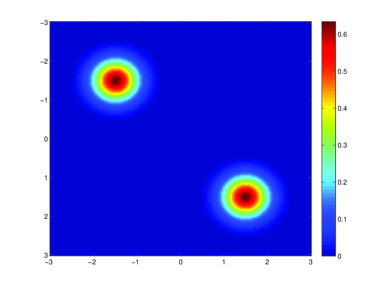
Figure 1: The distribution of the input $\rho$.

We choose the center and radius $(x_{0},R)$ which helps to define $G(\rho)$ as $x_{0}=(0,0),R=1$. Figure 5.1 gives the optimizer $\tilde{\Phi}$ (left) in (3.4) and its gradient $\nabla_{x}\tilde{\Phi}$ (right) computed using Algorithm 1 when $t=1$ in the Hamiltonian. The gradient $\nabla_{x}\tilde{\Phi}$ generates the final kick of the drift for the masses to be flown accordingly.

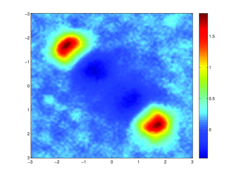
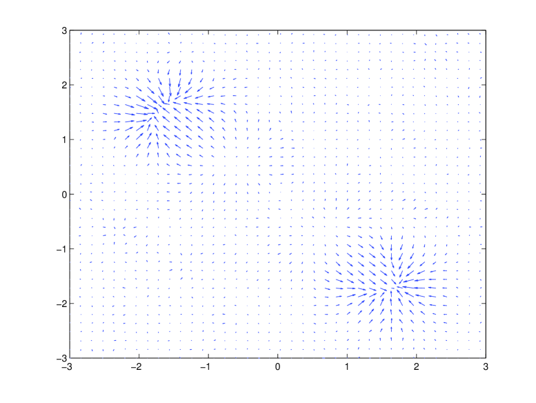
Figure 2: Left: optimizer $\tilde{\Phi}$ in $U(t,\rho)$ in (LABEL:lala_hopf), right: vector field $\nabla_{x}\tilde{\Phi}$.

In Figure 5.1, we plot the distributions $\rho(t,x)$ for different $t=0,0.2,0.4,0.6,0.8,1.0$. It describes the transportation of the masses according to the flow generated by the gradient of $\Phi(t,x)$ at different times $t$.

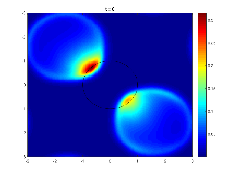
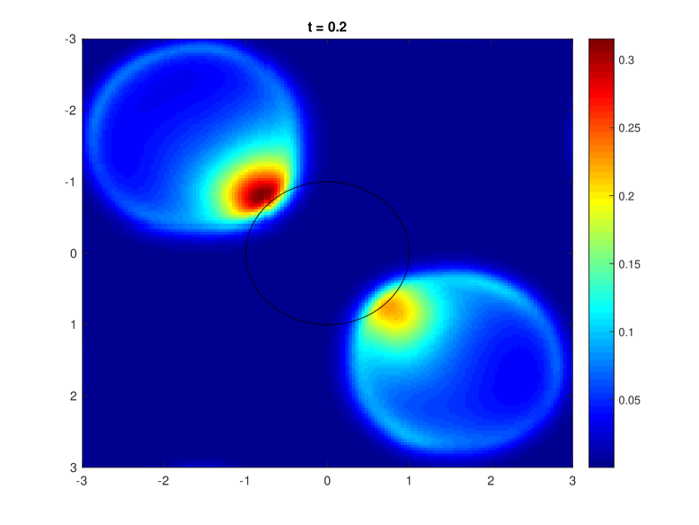
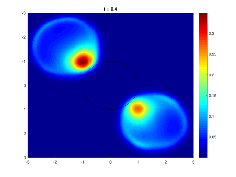
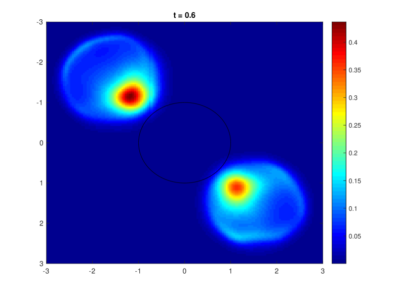
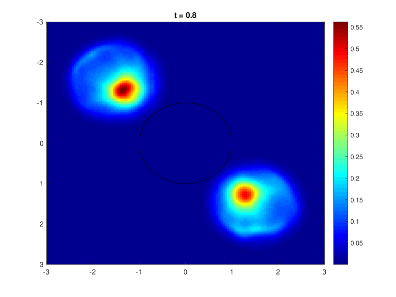
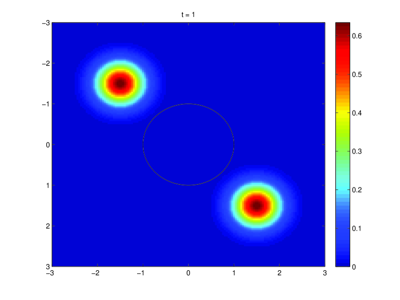
Figure 3: The distribution $\rho(t,x)$ generating the convection on the mass for different $t=0,0.2,0.4,0.6,0.8,1.0$. The black circle is the boundary of $B_{1}(0)$.

From the figures, we can see that our proposed method identifies simultaneously the two non-unique points closets from two mass lumps at antipodal positions to the ball in the center. In particular, the projected measure is the average of the two Dirac masses at the boundary of the circle, where each of them is the closest point of the mass lumps. The algorithm uses reversed time, and the reconstruction moves from the points on the balls to the two respective masses.

Example 5.2.

In this example, we consider the Hamiltonian $H_{1}$ above and the input distribution $\rho(x)$ as follows:

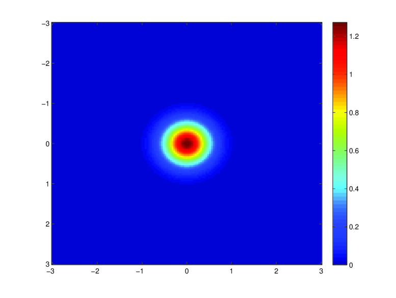
Figure 4: The distribution of the input $\rho$.

We choose the center and radius $(x_{0},R)$, which helps to define $G(\rho)$ as $x_{0}=(3,0),R=2$. Since this is a torus, the mass sees a “non-convex” object from both sides from afar. Figure 5.2 gives the optimizer $\tilde{\Phi}$ (left) in (LABEL:lala_hopf) and its gradient $\nabla_{x}\tilde{\Phi}$ (right) computed using Algorithm 1 when $t=1$ in the Hamiltonian. We fix $L_{i}=2$ in Algorithm 1.

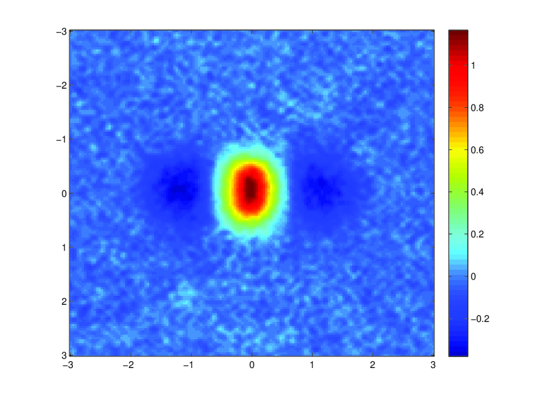
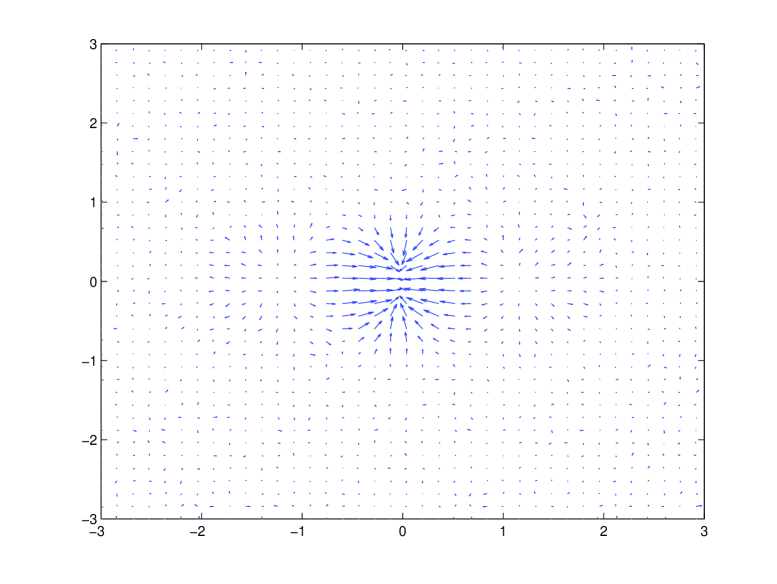
Figure 5: Left: optimizer $\tilde{\Phi}$ in $U(t,\rho)$ in (LABEL:lala_hopf), right: vector field $\nabla_{x}\tilde{\Phi}$.

In Figure 5.2, we plot the distributions $\rho(t,x)$ for different $t=0,0.2,0.4,0.6,0.8,1.0$.

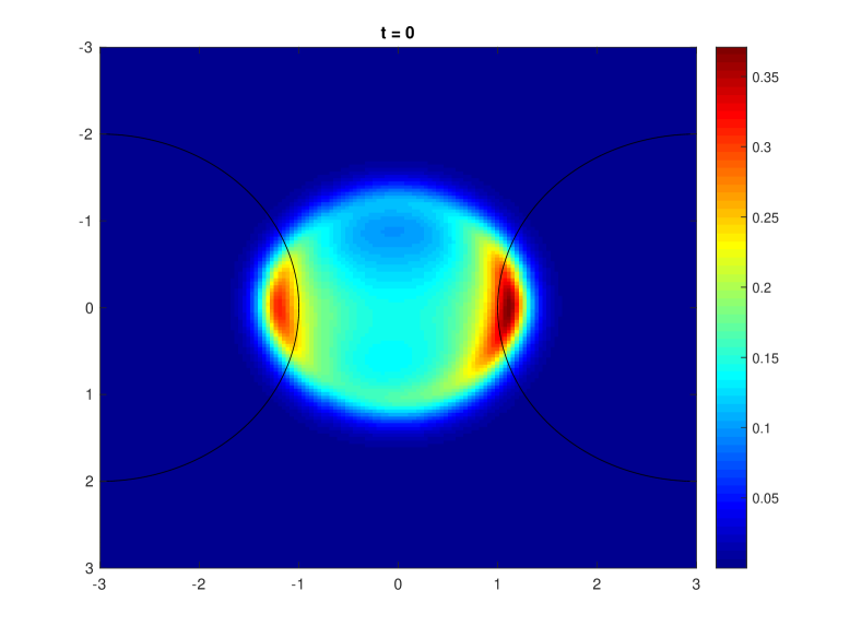
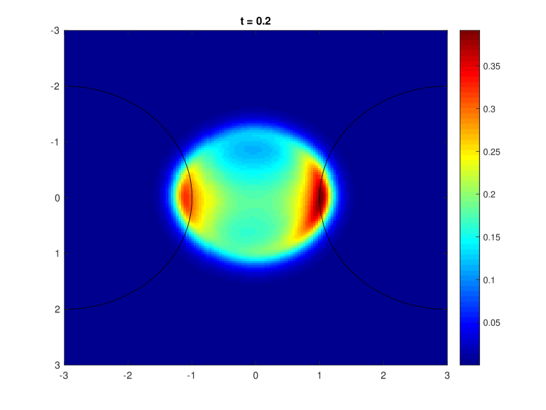
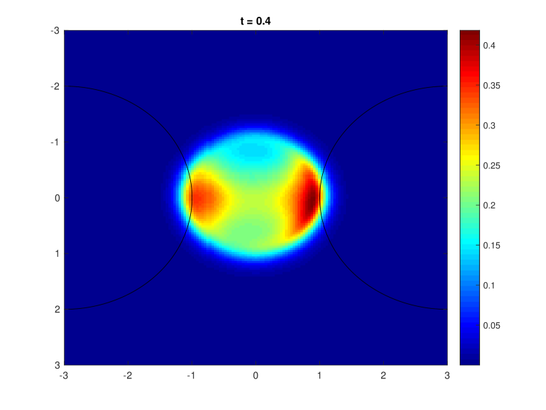
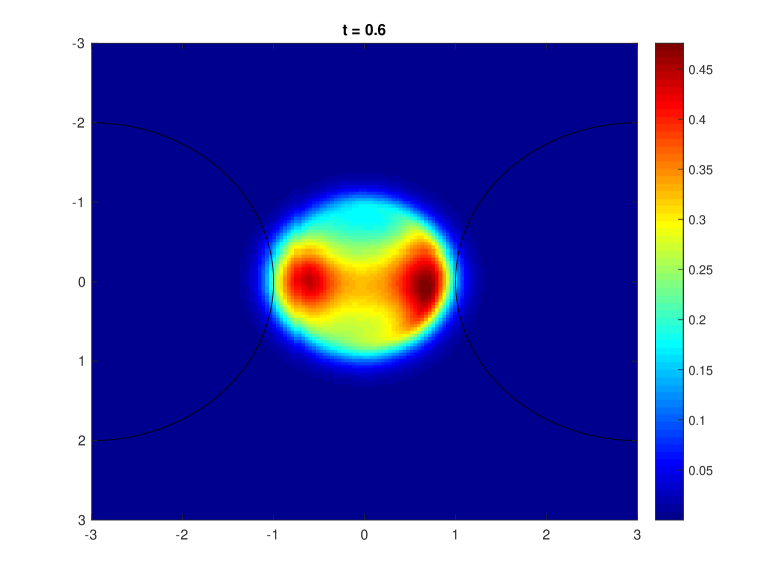
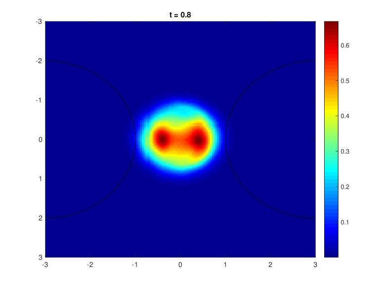
Figure 6: The distribution $\rho(t,x)$ generating the convection on the mass for different $t=0,0.2,0.4,0.6,0.8,1.0$. The black circle is the boundary of $B_{1}(0)$.

In this example, our method accurately finds the projections of a mass to the two non-unique closest points on the “non-convex” body (which is in fact a ball ”split” in two). In particular, the flow of the mass splits into two opposite directions; each brings half of the densities to the boundary of the target body.

Example 5.3.

In this example, we consider the non-convex Hamiltonian $H_{3}$ above and the input distribution $\rho(x)$ in Figure 5.3.

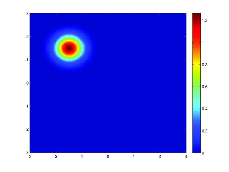
Figure 7: The distribution of the input $\rho$.

In order to compute the absolute value in the conservation law in a stable way, we replace the function with a soft absolute value as follows

$$\text{soft-abs-value}(x):=\frac{2}{\pi}\arctan(cx)\,,$$

where we choose $c=20$. With this regularization, the Hamiltonian under consideration is actually

$$H_{3,c}(p):=H_{c}(p_{1})+H_{c}(p_{2})$$

where

$$H_{c}(s)=\frac{2}{\pi}s\arctan(s)-\frac{1}{c\pi}\log(1+c^{2}s^{2})\,,$$

and thus the Lagrangian cost functional is

$$L_{3,c}(v):=L_{c}(v_{1})+L_{c}(v_{2}),$$

where

$$L_{c}(t)=\begin{cases}\frac{1}{c\pi}\log\left(\sec^{2}\left(\frac{\pi t}{2}\right)\right)&\text{ if }|t|<1\,,\\ \infty&\text{ if }|t|\geq 1\,.\\ \end{cases}$$

As in Example 1, we choose the center and radius $(x_{0},R)$ which helps to define $G(\rho)$ as $x_{0}=(0,0),R=1$. Figure 5.4 gives the optimizer $\tilde{\Phi}$ (left) in (3.4) and its gradient $\nabla_{x}\tilde{\Phi}$ (right) computed using Algorithm 1 when $t=1$ in the Hamiltonian.

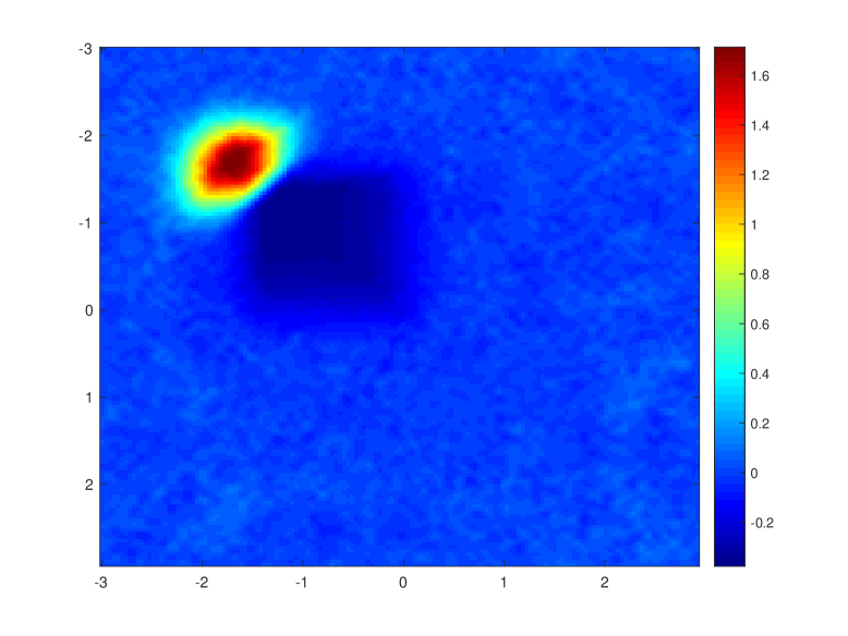
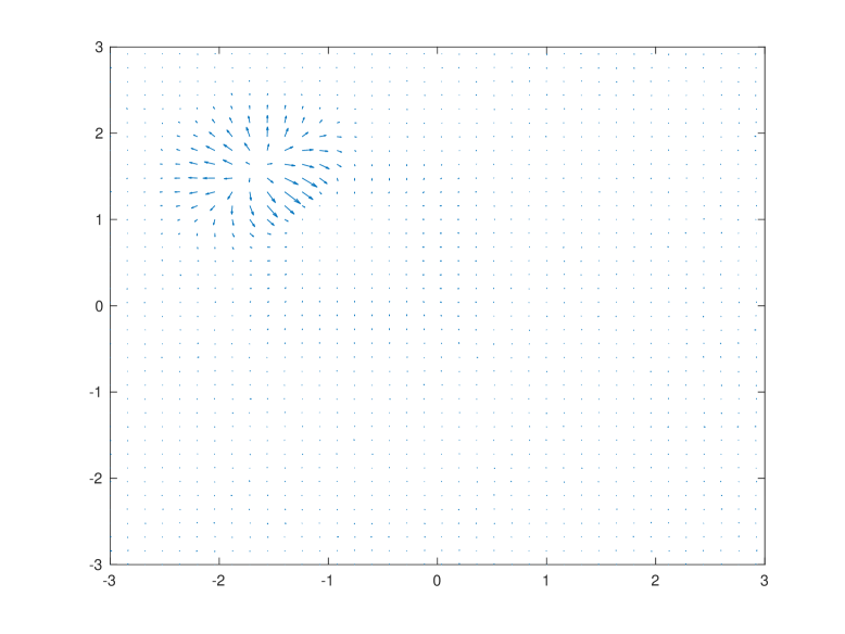
Figure 8: Left: optimizer $\tilde{\Phi}$ in $U(t,\rho)$ in (LABEL:lala_hopf), right: vector field $\nabla_{x}\tilde{\Phi}$.

Figure 5.4 plots the distributions $\rho(t,x)$ for different $t=0,0.2,0.4,0.6,0.8,1.0$.

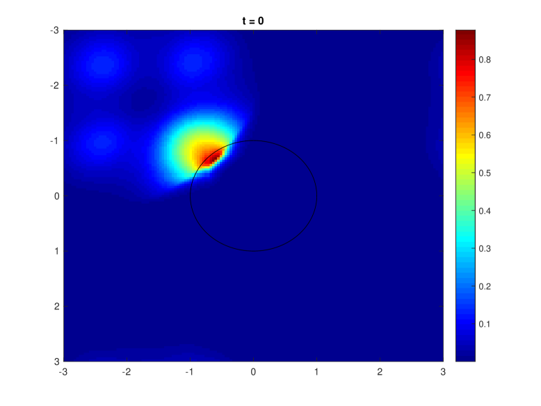
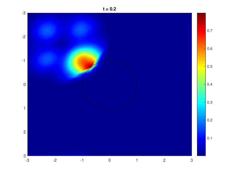
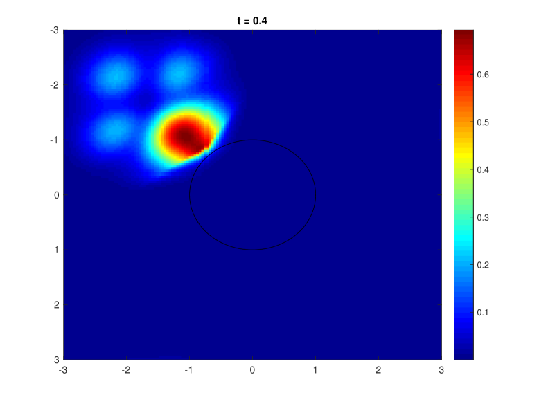
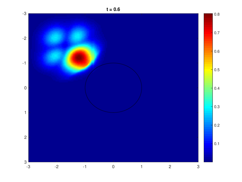
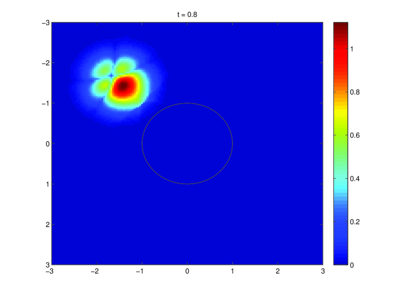
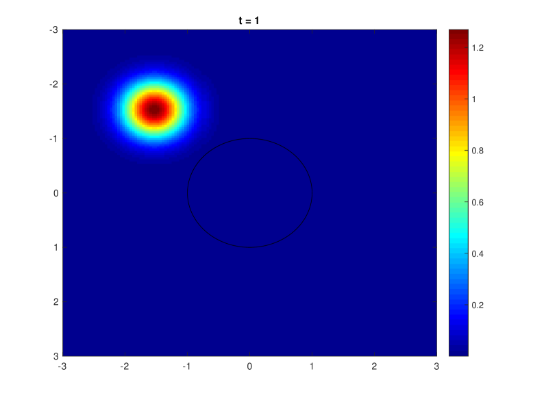
Figure 9: The distribution $\rho(t,x)$ generating the convection on the mass for different $t=0,0.2,0.4,0.6,0.8,1.0$. The black circle is the boundary of $B_{1}(0)$.

We identify reachability of the measure to the boundary of the ball w.r.t. to the $l_{1}$ Hamiltonian. With our choice of regularization, we, however, see a defect in our numerical computation: there are three small tails that are left behind in the conservation law as the mass is moving since the exact cutoff of the absolute value is regularized. Nonetheless, the solution makes perfect sense in term of identifying reachability.

Example 5.4.

In this example, we consider the non-convex Hamiltonian $H_{2}$ above and the input distribution $\rho(x)$ the same as in Example 1 in Figure 5.1.

Again, we choose the center and radius $(x_{0},R)$, which helps to define $G(\rho)$ as $x_{0}=(0,0),R=1$. Figure 5.4 gives the optimizer $\tilde{\Phi}$ (left) in (3.4) and its gradient $\nabla_{x}\tilde{\Phi}$ (right)computed using Algorithm 1 when $t=1$ in the Hamiltonian.

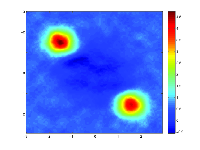
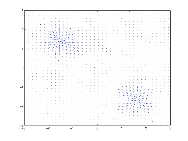
Figure 10: Left: optimizer $\tilde{\Phi}$ in $U(t,\rho)$ in (LABEL:lala_hopf), right: vector field $\nabla_{x}\tilde{\Phi}$.

Figure 5.4 plots the distributions $\rho(t,x)$ for different $t=0,0.2,0.4,0.6,0.8,1.0$.

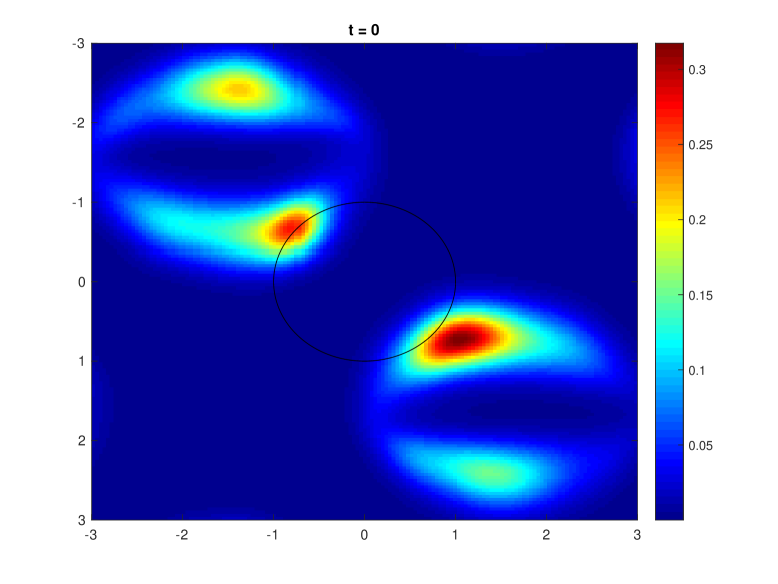
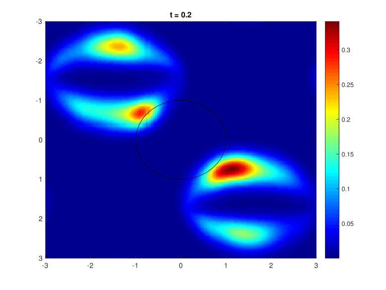
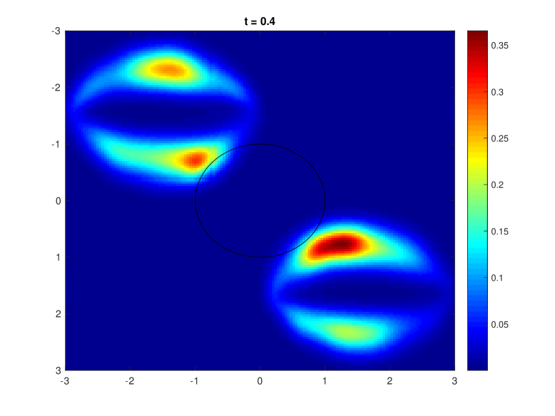
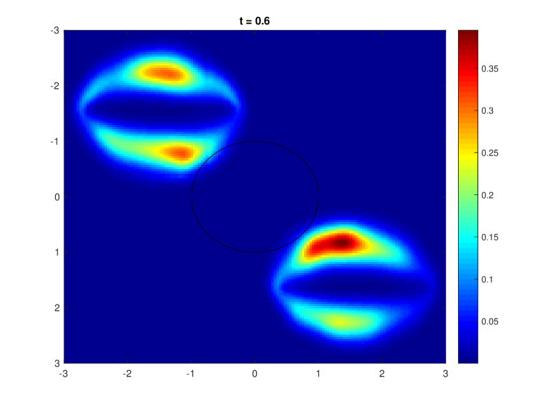
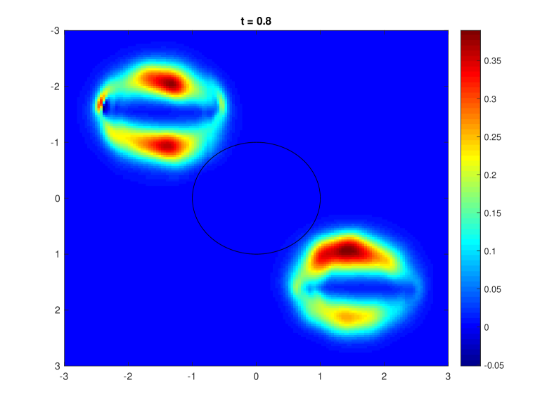
Figure 11: The distribution $\rho(t,x)$ generating the convection on the mass for different $t=0,0.2,0.4,0.6,0.8,1.0$. The black circle is the boundary of $B_{1}(0)$.

We can see the competing nature of the Hamiltonian, where one part of the Hamiltonian tries to drift the mass to the ball inward along one direction, while the other part of the Hamiltonian tries to drift the mass away along another direction. This tears each mass lump apart into two lumps. Although the problem has not been fully understood mathematically, the numerical behavior of the solution shows the competing nature of a differential game problem in the mean field setting.

6 Discussions

To summarize, we propose a generalized Hopf formula for potential mean field games. Our algorithm inherits main ideas in optimal transport on graphs and the Hopf formula for state-dependent optimal control problems.

Compared to the existing methods, the advantage of the proposed algorithm is three fold. First, the Hopf formula in density space introduces a minimization with variables depending on solely spatial grids. It has a lower complexity than the original optimal control problem. Second, the Hopf formula gives a simple parameterization for boundary problems in NE. This parameterization helps us design a simple first-order gradient descent method. This property allows us to compute the case of nonconvex Hamiltonians efficiently. Finally, our spatial discretization follows the dual of optimal transport on graphs. Hence, it is approximately discrete time reversible. This property conserves the primal-dual structure of potential mean field games.

We notice that the Hopf formula in density space appears to go beyond monotonicity conditions and give legitimate numerical results, as shown in Section 5. Although it is beyond the scope of this paper, it is interesting to search for the precise conditions for the validity of the Hopf formula. Also, our current study only considers potential games without noise perturbations in players’ decision processes. We will extend it to compute NEs for general non-potential games in future work.

References

- [1] Y. Achdou, F. Camilli, and I. Capuzzo-Dolcetta. Mean Field Games: Numerical Methods for the Planning Problem. SIAM Journal on Control and Optimization, 50(1):77–109, 2012.
- [2] Y. Achdou, F. Camilli, and I. Capuzzo-Dolcetta. Mean Field Games: Convergence of a Finite Difference Method. SIAM Journal on Numerical Analysis, 51(5):2585–2612, 2013.
- [3] Y. Achdou and I. Capuzzo-Dolcetta. Mean Field Games: Numerical Methods. SIAM Journal on Numerical Analysis, 48(3):1136–1162, 2010.
- [4] N. Almulla, R. Ferreira, and D. Gomes. Two Numerical Approaches to Stationary Mean-Field Games. Dynamic Games and Applications, 7(4):657–682, 2017.
- [5] J.-D. Benamou and Y. Brenier. A computational fluid mechanics solution to the Monge-Kantorovich mass transfer problem. Numerische Mathematik, 84(3):375–393, 2000.
- [6] J.-D. Benamou and G. Carlier. Augmented Lagrangian Methods for Transport Optimization, Mean Field Games and Degenerate Elliptic Equations. Journal of Optimization Theory and Applications, 167(1):1–26, 2015.
- [7] J.-D. Benamou, G. Carlier, M. Cuturi, L. Nenna, and G. Peyré. Iterative Bregman Projections for Regularized Transportation Problems. SIAM Journal on Scientific Computing, 37(2):A1111–A1138, 2015.
- [8] P. Cardaliaguet, F. Delarue, J.-M. Lasry, and P.-L. Lions. The master equation and the convergence problem in mean field games. arXiv:1509.02505 [math], 2015.
- [9] S.-N. Chow, L. Dieci, W. Li, and H. Zhou. Entropy dissipation semi-discretization schemes for Fokker-Planck equations. arXiv:1608.02628 [math], 2016.
- [10] S.-N. Chow, W. Li, and H. Zhou. A discrete Schrodinger equation via optimal transport on graphs. arXiv:1705.07583 [math], 2017.
- [11] S.-N. Chow, W. Li, and H. Zhou. Entropy dissipation of Fokker-Planck equations on graphs. arXiv:1701.04841 [math], 2017.
- [12] Y. T. Chow, J. Darbon, S. Osher, and W. Yin. Algorithm for Overcoming the Curse of Dimensionality for State-dependent Hamilton-Jacobi equations. arXiv:1704.02524 [math], 2017.
- [13] Y. T. Chow, J. Darbon, S. Osher, and W. Yin. Algorithm for Overcoming the Curse of Dimensionality For Time-Dependent Non-convex Hamilton–Jacobi Equations Arising From Optimal Control and Differential Games Problems. Journal of Scientific Computing, 73(2-3):617–643, 2017.
- [14] Y. T. Chow, J. Darbon, S. Osher, and W. Yin. Algorithm for Overcoming the Curse of Dimensionality For Time-Dependent Non-convex Hamilton–Jacobi Equations Arising From Optimal Control and Differential Games Problems. Journal of Scientific Computing, 73(2-3):617–643, 2017.
- [15] J. Darbon and S. Osher. Algorithms for overcoming the curse of dimensionality for certain Hamilton–Jacobi equations arising in control theory and elsewhere. Research in the Mathematical Sciences, 3(1), 2016.
- [16] W. Gangbo, W. Li, and C. Mou. Geodesic of minimal length in the set of probability measures on graphs. arXiv:1712.09266 [math], 2017.
- [17] W. Gangbo, T. Nguyen, and A. Tudorascu. Hamilton-Jacobi Equations in the Wasserstein Space. 2008.
- [18] W. Gangbo and A. Swiech. Existence of a solution to an equation arising from the theory of Mean Field Games. Journal of Differential Equations, 259(11):6573–6643, 2015.
- [19] O. Guéant, J.-M. Lasry, and P.-L. Lions. Mean Field Games and Applications. In J.-M. Morel, F. Takens, and B. Teissier, editors, Paris-Princeton Lectures on Mathematical Finance 2010, volume 2003, pages 205–266. Springer Berlin Heidelberg, Berlin, Heidelberg, 2011.
- [20] M. Huang, R. P. Malhamé, and P. E. Caines. Large population stochastic dynamic games: Closed-loop McKean-Vlasov systems and the Nash certainty equivalence principle. Communications in Information & Systems, 6(3):221–252, 2006.
- [21] H. Komiya. Elementary proof for Sion’s minimax theorem. Kodai Mathematical Journal, 11(1):5–7, 1988.
- [22] J.-M. Lasry and P.-L. Lions. Mean field games. Japanese Journal of Mathematics, 2(1):229–260, 2007.
- [23] W. Li, P. Yin, and S. Osher. Computations of Optimal Transport Distance with Fisher Information Regularization. Journal of Scientific Computing, 2017.
- [24] D. Monderer and L. S. Shapley. Potential Games. Games and Economic Behavior, 14(1):124–143, 1996.
- [25] E. Nelson. Derivation of the Schrödinger Equation from Newtonian Mechanics. Physical Review, 150(4):1079–1085, 1966.
- [26] M. Sion. On general minimax theorems. Pacific Journal of Mathematics, 8(1):171–176, 1958.
- [27] C. Villani. Optimal Transport: Old and New. Number 338 in Grundlehren der mathematischen Wissenschaften. Springer, Berlin, 2009.
- [28] I. Yegorov and P. Dower. Perspectives on characteristics based curse-of-dimensionality-free numerical approaches for solving Hamilton-Jacobi equations. arXiv:1711.03314 [math], 2017.