A software framework for embedded nonlinear model predictive control using a gradient-based augmented Lagrangian approach (GRAMPC)

Abstract

A nonlinear MPC framework is presented that is suitable for dynamical systems with sampling times in the (sub)millisecond range and that allows for an efficient implementation on embedded hardware. The algorithm is based on an augmented Lagrangian formulation with a tailored gradient method for the inner minimization problem. The algorithm is implemented in the software framework GRAMPC and is a fundamental revision of an earlier version. Detailed performance results are presented for a test set of benchmark problems and in comparison to other nonlinear MPC packages. In addition, runtime results and memory requirements for GRAMPC on ECU level demonstrate its applicability on embedded hardware.

1 Introduction

Model predictive control (MPC) is one of the most popular advanced control methods due to its ability to handle linear and nonlinear systems with constraints and multiple inputs. The well-known challenge of MPC is the numerical effort that is required to solve the underlying optimal control problem (OCP) online. In the recent past, however, the methodological as well as algorithmic development of MPC for linear and nonlinear systems has matured to a point that MPC nowadays can be applied to highly dynamical problems in real-time. Most approaches of real-time MPC either rely on suboptimal solution strategies Scokaert:TAC:1999 ; Diehl:IEE:2004 ; Graichen:TAC:2010 and/or use tailored optimization algorithms to optimize the computational efficiency.

Particularly for linear systems, the MPC problem can be reduced to a quadratic problem, for which the optimal control over the admissible polyhedral set can be precomputed. This results in an explicit MPC strategy with minimal computational effort for the online implementation Bemporad:TAC:2002 ; Bemporad:AUT:2002 , though this approach is typically limited to a small number of state and control variables. An alternative to explicit MPC is the online active set method Ferreau:IJRNC:2008 that takes advantage of the receding horizon property of MPC in the sense that typically only a small number of constraints becomes active or inactive from one MPC step to the next.

In contrast to active set strategies, interior point methods relax the complementary conditions for the constraints and therefore solve a relaxed set of optimality conditions in the interior of the admissable constraint set. The MPC software packages FORCES (PRO) Domahidi:CDC:2012 and fast_mpc Wang:CST:2010 employ interior point methods for linear MPC problems. An alternative to active set and interior point methods are accelerated gradient methods Richter:TAC:2012 that originally go back to Nesterov’s fast gradient method for convex problems Nesterov:2003 . A corresponding software package for linear MPC is FiOrdOs Jones:NPCC:2012 .

For nonlinear systems, one of the first real-time MPC algorithms was the continuation/GMRES method Ohtsuka:AUT:2004 that solves the optimality conditions of the underlying optimal control problem based on a continuation strategy. The well-known ACADO Toolkit Houska2011 uses the above-mentioned active set strategy in combination with a real-time iteration scheme to efficiently solve nonlinear MPC problems. Another recently presented MPC toolkit is VIATOC Kalmari2015 that employs a projected gradient method to solve the time-discretized, linearized MPC problem.

Besides the real-time aspect of MPC, a current focus of research is on embedded MPC, i.e. the neat integration of MPC on embedded hardware with limited ressources. This might be field programmable gate arrays (FPGA) Ling:IFACWC:2008 ; Kaepernick:UKACC:2014 ; Hartley:OCAM:2015 , programmable logic controllers (PLC) in standard automation systems Kufoalor:MED:2014 ; Kaepernick:IFACWC:2014 or electronic control units (ECU) in automotive applications Mesmer:CST:2018 . For embedded MPC, several challenges arise in addition to the real-time demand. For instance, numerical robustness even at low computational accuracy and tolerance against infeasibility are important aspects as well as the ability to provide fast, possibly suboptimal iterates with minimal computational demand. In this regard, it is also desirable to satisfy the system dynamics in the single MPC iterations in order to maintain dynamically consistent iterates. Low code complexity for portability and a small memory footprint are further important aspects to allow for an efficient implementation of MPC on embedded hardware. The latter aspects, in particular, require the usage of streamlined, self-contained code rather than highly complex MPC algorithms. To meet these challenges, gradient-based algorithms become popular choices due to their general simplicity and low computational complexity Giselsson:IFACWC:2014 ; Kouzoupis:EEC:2015 ; Necoara:SCL:2015 .

Following this motivation, this paper presents a software framework for nonlinear MPC that can be efficiently used for embedded control of nonlinear and highly dynamical systems with sampling times in the (sub)millisecond range. The presented framework is a fundamental revision of the MPC toolbox GRAMPC Kaepernick2014 (Gradient-Based MPC – [græmp^′si:]) that was originally developed for nonlinear systems with pure input constraints. The revised algorithm of GRAMPC presented in this paper allows to account for general nonlinear equality and inequality constraints, as well as terminal constraints. Beside “classical” MPC, the toolbox can be applied to MPC on shrinking horizon, general optimal control problems, moving horizon estimation and parameter optimization problems including free end time problems. The new algorithm is based on an augmented Lagrangian formulation in connection with a real-time gradient method and tailored line search and multiplier update strategies that are optimized for a time and memory efficient implementation on embedded hardware. The performance and effectiveness of augmented Lagrangian methods for embedded nonlinear MPC was recently demonstrated for various application examples on rapid prototyping and ECU hardware level Harder:AIM:2017 ; Mesmer:CST:2018 ; Englert:CEP:2018 . Beside the presentation of the augmented Lagrangian algorithm and the general usage of GRAMPC, the paper compares its performance to the nonlinear MPC toolkits ACADO and VIATOC for different benchmark problems. Moreover, runtime results are presented for GRAMPC on dSPACE and ECU level including its memory footprint to demonstrate its applicability on embedded hardware.

The paper is organized as follows. Section 2 presents the general problem formulation and exemplarily illustrates its application to model predictive control and moving horizon estimation. Section 3 describes the augmented Lagrangian framework in combination with a gradient method for the inner minimization problem. Section 4 gives an overview on the structure and usage of GRAMPC. Section 5 evaluates the performance of GRAMPC for different benchmark problems and in comparison to ACADO and VIATOC, before Section 6 closes the paper.

Some norms are used inside the paper, in particular in Section 3. The Euclidean norm of a vector $\boldsymbol{x}\in\mathbb{R}^{n}$ is denoted by $\|\boldsymbol{x}\|_{2}$, the weighted quadratic norm by $\|\boldsymbol{x}\|_{\boldsymbol{Q}}=(\boldsymbol{x}^{\mathsf{T}}\boldsymbol{Q}\boldsymbol{x})^{1/2}$ for some positive definite matrix $\boldsymbol{Q}$, and the scalar product of two vectors $\boldsymbol{x},\boldsymbol{y}\in\mathbb{R}^{n}$ is defined as $\langle\boldsymbol{x},\boldsymbol{y}\rangle=\boldsymbol{x}^{\mathsf{T}}\boldsymbol{y}$. For a time function $\boldsymbol{x}(t)$, $t\in[0,T]$ with $T<\infty$, the vector-valued $L^{2}$-norm is defined by $\|\boldsymbol{x}\|_{L_{2}}=\big{(}\sum_{i=1}^{n}\|x_{i}\|_{L_{2}}\big{)}^{1/2}$ with $\|x_{i}\|_{L_{2}}=\big{(}\int_{0}^{T}\!x_{i}^{2}(t)\,{\rm d}t\big{)}^{1/2}$. The supremum-norm is defined componentwise in the sense of $\|\boldsymbol{x}\|_{L_{\infty}}=\big{[}\|x_{1}\|_{L_{\infty}}\ldots\|x_{n}\|_{L_{\infty}}\big{]}^{\mathsf{T}}$ with $\|x_{i}\|_{L_{\infty}}=\sup_{t\in[0,T]}|x_{i}(t)|$. The inner product is denoted by $\langle\boldsymbol{x},\boldsymbol{y}\rangle=\int_{0}^{T}\!\boldsymbol{x}^{\mathsf{T}}(t)\boldsymbol{y}(t)\,{\rm d}t$ using the same (overloaded) $\langle\,\rangle$-notation as in the vector case. Moreover, function arguments (such as time $t$) might be omitted in the text for the sake of enhancing readability.

2 Problem formulation

This section describes the class of optimal control problems that can be solved by GRAMPC. The framework is especially suitable for model predictive control and moving horizon estimation, as the numerical solution method is tailored to embedded applications. Nevertheless, GRAMPC can be used to solve general optimal control problems or parameter optimization problems as well.

2.1 Optimal control problem

GRAMPC solves nonlinear constrained optimal control problems with fixed or free end time and potentially unknown parameters. Consequently, the most generic problem formulation that can be adressed by GRAMPC is given by

$$\!\!\!\min_{\boldsymbol{u},\boldsymbol{p},T}\quad J(\boldsymbol{u},\boldsymbol{p},T;\boldsymbol{x}_{0})=V(\boldsymbol{x}(T),\boldsymbol{p},T)+\int_{0}^{T}l(\boldsymbol{x}(t),\boldsymbol{u}(t),\boldsymbol{p},t)\,{\rm d}t$$ (1a)

s.t. $$\boldsymbol{M}\boldsymbol{\dot{x}}(t)=\boldsymbol{f}(\boldsymbol{x}(t),\boldsymbol{u}(t),\boldsymbol{p},t)\,,\quad\boldsymbol{x}(0)=\boldsymbol{x}_{0}$$ (1b)

$$\boldsymbol{g}(\boldsymbol{x}(t),\boldsymbol{u}(t),\boldsymbol{p},t)=\boldsymbol{0}\,,\quad\boldsymbol{g}_{T}(\boldsymbol{x}(T),\boldsymbol{p},T)=\boldsymbol{0}$$ (1c)

$$\boldsymbol{h}(\boldsymbol{x}(t),\boldsymbol{u}(t),\boldsymbol{p},t)\leq\boldsymbol{0}\,,\quad\boldsymbol{h}_{T}(\boldsymbol{x}(T),\boldsymbol{p},T)\leq\boldsymbol{0}$$ (1d)

$$\boldsymbol{u}(t)\in\left[\boldsymbol{u}_{\min},\boldsymbol{u}_{\max}\right]$$ (1e)

$$\boldsymbol{p}\in\left[\boldsymbol{p}_{\min},\boldsymbol{p}_{\max}\right]\,,\quad T\in\left[T_{\min},T_{\max}\right]$$ (1f)

with state $\boldsymbol{x}\in\mathbb{R}^{N_{\boldsymbol{x}}}$, control $\boldsymbol{u}\in\mathbb{R}^{N_{\boldsymbol{u}}}$, parameters $\boldsymbol{p}\in\mathbb{R}^{N_{\boldsymbol{p}}}$ and end time $T\in\mathbb{R}$. The cost to be minimized (1a) consists of the terminal and integral cost functions $V:\mathbb{R}^{N_{\boldsymbol{x}}}\times\mathbb{R}^{N_{\boldsymbol{p}}}\times\mathbb{R}\rightarrow\mathbb{R}$ and $l:\mathbb{R}^{N_{\boldsymbol{x}}}\times\mathbb{R}^{N_{\boldsymbol{u}}}\times\mathbb{R}^{N_{\boldsymbol{p}}}\times\mathbb{R}\rightarrow\mathbb{R}$, respectively. The dynamics (1b) are given in semi-implicit form with the (constant) mass matrix $\boldsymbol{M}$, the nonlinear system function $\boldsymbol{f}:\mathbb{R}^{N_{\boldsymbol{x}}}\times\mathbb{R}^{N_{\boldsymbol{u}}}\times\mathbb{R}^{N_{\boldsymbol{p}}}\times\mathbb{R}\rightarrow\mathbb{R}^{N_{x}}$, and the initial state $\boldsymbol{x}_{0}$. The system class (1b) includes standard ordinary differential equations for $\boldsymbol{M}=\boldsymbol{I}$ as well as (index-1) differential-algebraic equations with singular mass matrix $\boldsymbol{M}$. In addition, (1c) and (1d) account for equality and inequality constraints $\boldsymbol{g}:\mathbb{R}^{N_{\boldsymbol{x}}}\times\mathbb{R}^{N_{\boldsymbol{u}}}\times\mathbb{R}^{N_{\boldsymbol{p}}}\times\mathbb{R}\rightarrow\mathbb{R}^{N_{\boldsymbol{g}}}$ and $\boldsymbol{h}:\mathbb{R}^{N_{\boldsymbol{x}}}\times\mathbb{R}^{N_{\boldsymbol{u}}}\times\mathbb{R}^{N_{\boldsymbol{p}}}\times\mathbb{R}\rightarrow\mathbb{R}^{N_{\boldsymbol{h}}}$ as well as for the corresponding terminal constraints $\boldsymbol{g}_{T}:\mathbb{R}^{N_{\boldsymbol{x}}}\times\mathbb{R}^{N_{\boldsymbol{p}}}\times\mathbb{R}\rightarrow\mathbb{R}^{N_{\boldsymbol{g}_{T}}}$ and $\boldsymbol{h}_{T}:\mathbb{R}^{N_{\boldsymbol{x}}}\times\mathbb{R}^{N_{\boldsymbol{p}}}\times\mathbb{R}\rightarrow\mathbb{R}^{N_{\boldsymbol{h}_{T}}}$, respectively. Finally, (1e) and (1f) represent box constraints for the optimization variables $\boldsymbol{u}=\boldsymbol{u}(t)$, $\boldsymbol{p}$ and $T$ (if applicable).

In comparison to the previous version of the GRAMPC toolbox Kaepernick2014 , the problem formulation (1) supports optimization with respect to parameters, a free end time, general state-dependent equality and inequality constraints, as well as terminal constraints. Furthermore, semi-implicit dynamics with a constant mass matrix $\boldsymbol{M}$ can be handled using the Rosenbrock solver RODAS Hairer:Book:1996:Stiff as numerical integrator. This extends the range of possible applications besides MPC to general optimal control, parameter optimization, and moving horizon estimation. However, the primary target is embedded model predictive control of nonlinear systems, as the numerical solution algorithm is optimized for time and memory efficiency.

2.2 Application to model predictive control

Model predictive control relies on the iterative solution of an optimal control problem of the form

$$\min_{\boldsymbol{u}}\quad J(\boldsymbol{u};\boldsymbol{x}_{k})=V(\boldsymbol{x}(T))+\int_{0}^{T}l(\boldsymbol{x}(\tau),\boldsymbol{u}(\tau),\tau)\,{\rm d}\tau$$ (2a)

 s.t. $$\boldsymbol{M}\boldsymbol{\dot{x}}(\tau)=\boldsymbol{f}(\boldsymbol{x}(\tau),\boldsymbol{u}(\tau),t_{k}+\tau)\,,\quad \boldsymbol{x}(0) =\boldsymbol{x}_{k}$$ (2b)

$$\boldsymbol{x}(\tau)\in\left[\boldsymbol{x}_{\min},\boldsymbol{x}_{\max}\right]\,,\quad \boldsymbol{x}(T) \in\Omega_{\beta}$$ (2c)

$$\boldsymbol{u}(\tau)\in\left[\boldsymbol{u}_{\min},\boldsymbol{u}_{\max}\right]$$ (2d)

with the MPC-internal time coordinate $\tau\in[0,T]$ over the prediction horizon $T$. The initial state value $\boldsymbol{x}_{k}$ is the measured or estimated system state at the current sampling instant $t_{k}=t_{0}+k\Delta t$, $k\in\mathbb{N}$ with sampling time $0<\Delta t\leq T$. The first part of the computed control trajectory $\boldsymbol{u}(\tau)$, $\tau\in[0,\Delta t)$ is used as control input for the actual plant over the time interval $t\in[t_{k},t_{k+1})$, before OCP (2) is solved again with the new initial state $\boldsymbol{x}_{k+1}$.

A popular choice of the cost functional (2a) is the quadratic form

$$V(\boldsymbol{x})=\|\boldsymbol{x}-\boldsymbol{x}_{\text{des}}\|^{2}_{\boldsymbol{P}}\,,\quad l(\boldsymbol{x},\boldsymbol{u})=\|\boldsymbol{x}-\boldsymbol{x}_{\text{des}}\|_{\boldsymbol{Q}}^{2}+\|\boldsymbol{u}-\boldsymbol{u}_{\text{des}}\|_{\boldsymbol{R}}^{2}$$ (3)

with the desired setpoint $(\boldsymbol{x}_{\text{des}},\boldsymbol{u}_{\text{des}})$ and the positive (semi-)definite matrices $\boldsymbol{P}$, $\boldsymbol{Q}$, $\boldsymbol{R}$. Stability is often ensured in MPC by imposing a terminal constraint $\boldsymbol{x}(T)\in\Omega_{\beta}$, where the set $\Omega_{\beta}=\{\boldsymbol{x}\in\mathbb{R}^{N_{\boldsymbol{x}}}\,|\,V(\boldsymbol{x})\leq\beta\}$ for some $\beta>0$ is defined in terms of the terminal cost $V(\boldsymbol{x})$ that can be computed from solving a Lyapunov or Riccati equation that renders the set $\Omega_{\beta}$ invariant under a local feedback law Chen:AUT:1998 ; Mayne:AUT:2000 . In view of the OCP formulation (1), the terminal region as well as general box constraints on the state as given in (2c) can be expressed as

$$\boldsymbol{h}(\boldsymbol{x})=\begin{bmatrix}\boldsymbol{x}-\boldsymbol{x}_{\text{max}}\\ \boldsymbol{x}_{\text{min}}-\boldsymbol{x}\end{bmatrix}\leq\boldsymbol{0}\,,\quad\boldsymbol{h}_{T}(\boldsymbol{x})=V(\boldsymbol{x})-\beta\leq\boldsymbol{0}\,.$$ (4)

Note, however, that terminal constraints are often omitted in embedded or real-time MPC in order to minimize the computational effort Limon:TAC:2006 ; Graichen2010 ; Gruene:AUT:2013 . In particular, real-time feasibility is typically achieved by limiting the number of iterations per sampling step and using the current solution for warm starting in the next MPC step, in order to incrementally reduce the suboptimality over the runtime of the MPC Diehl:IEE:2004 ; Graichen2010 ; Graichen:AUT:2012 .

An alternative to the “classical” MPC formulation (2) is shrinking horizon MPC, see e.g. Diehl:SIAM:2005 ; Skaf:IJRNC:2010 ; Gruene:MTNS:2014 , where the horizon length $T$ is shortened over the MPC steps. This can be achieved by formulating the underlying OCP (2) as a free end time problem with a terminal constraint $\boldsymbol{g}_{T}(\boldsymbol{x}(T))=\boldsymbol{x}(T)-\boldsymbol{x}_{\text{des}}=\boldsymbol{0}$ to ensure that a desired setpoint $\boldsymbol{x}_{\text{des}}$ is reached in finite time instead of the asymptotic behavior of fixed-horizon MPC.

2.3 Application to moving horizon estimation

Moving horizon estimation (MHE) can be seen as the dual of MPC for state estimation problems. Similar to MPC, MHE relies on the online solution of a dynamic optimization problem of the form

$$\min_{\boldsymbol{\hat{x}}_{k}}\quad J(\boldsymbol{\hat{x}}_{k};\boldsymbol{u},\boldsymbol{y})=\int_{t_{k}-T}^{t_{k}}\|\boldsymbol{\hat{y}}(t)-\boldsymbol{y}(t)\|^{2}\,{\rm d}t$$ (5a)

 s.t. $$\boldsymbol{M}\boldsymbol{\dot{\hat{x}}}(t)=\boldsymbol{f}(\boldsymbol{\hat{x}}(t),\boldsymbol{u}(t),t)\,,\quad\boldsymbol{\hat{x}}(t_{k})=\boldsymbol{\hat{x}}_{k}$$ (5b)

$$\boldsymbol{\hat{y}}(t)=\boldsymbol{\sigma}(\boldsymbol{\hat{x}}(t))$$ (5c)

that depends on the history of the control $\boldsymbol{u}(t)$ and measured output $\boldsymbol{y}(t)$ over the past time window $[t_{k}-T,t_{k}]$. The solution of (5) yields the estimate $\boldsymbol{\hat{x}}_{k}$ of the current state $\boldsymbol{x}_{k}$ such that the estimated output function (5c) best matches the measured output $\boldsymbol{y}(t)$ over the past horizon $T$. Further constraints can be added to the formulation of (5) to incorporate a priori knowledge.

GRAMPC can be used for moving horizon estimation by handling the system state at the beginning of the estimation horizon as optimization variables, i.e. $\boldsymbol{p}=\boldsymbol{\hat{x}}(t_{k}-T)$. In addition, a time transformation is required to map $t\in[t_{k}-T,t_{k}]$ to the new time coordinate $\tau\in[0,T]$ along with the corresponding coordinate transformation

$$\boldsymbol{\tilde{x}}(\tau)=\boldsymbol{\hat{x}}(t_{k}\!-\!T\!+\!\tau)-\boldsymbol{p}\,,\quad\boldsymbol{\tilde{u}}(\tau)=\boldsymbol{u}(t_{k}\!-\!T\!+\!\tau)\,,\quad\boldsymbol{\tilde{y}}(\tau)=\boldsymbol{y}(t_{k}\!-\!T\!+\!\tau)$$ (6)

with the initial condition $\boldsymbol{\tilde{x}}(0)=\boldsymbol{0}$. The optimization problem (5) then becomes

$$\min_{\boldsymbol{p}}\quad J(\boldsymbol{p};\boldsymbol{\tilde{u}},\boldsymbol{\tilde{y}})=\int_{0}^{T}\|\boldsymbol{\hat{y}}(\tau)-\boldsymbol{\tilde{y}}(\tau)\|^{2}\,{\rm d}\tau$$ (7a)

s.t. $$\boldsymbol{M}\boldsymbol{\dot{\tilde{x}}}(\tau)=\boldsymbol{f}(\boldsymbol{\tilde{x}}(\tau)+\boldsymbol{p},\boldsymbol{\tilde{u}}(\tau),t_{k}\!-\!T\!+\!\tau)\,,\quad\boldsymbol{\tilde{x}}(0)=\boldsymbol{0}$$ (7b)

$$\boldsymbol{\hat{y}}(\tau)=\boldsymbol{\sigma}(\boldsymbol{\tilde{x}}(\tau)+\boldsymbol{p})\,.$$ (7c)

The solution $\boldsymbol{p}=\boldsymbol{\hat{x}}(t_{k}-T)$ of (7) and the coordinate transformation (6) are used to compute the current state estimate with

$$\boldsymbol{\hat{x}}_{k}=\boldsymbol{p}+\boldsymbol{\tilde{x}}(T)\,,$$ (8)

where $\boldsymbol{\tilde{x}}(T)$ is the end point of the state trajectory returned by GRAMPC. In the next sampling step, the parameters can be re-initialized with the predicted estimate $\boldsymbol{\hat{x}}(t_{k}-T+\Delta t)=\boldsymbol{p}+\boldsymbol{\tilde{x}}(\Delta t)$.

Note that the above time transformation can alternatively be reversed in order to directly estimate the current state $\boldsymbol{p}=\boldsymbol{\hat{x}}(t_{k})$. This, however, requires the reverse time integration of the dynamics, which is numerically unstable if the system is stable in forward time. Vice versa, a reverse time transformation is to be preferred for MHE of an unstable process.

3 Optimization algorithm

The optimization algorithm underlying GRAMPC uses an augmented Lagrangian formulation in combination with a real-time projected gradient method. Though SQP or interior point methods are typically superior in terms of convergence speed and accuracy, the augmented Lagrangian framework is able to rapidly provide a suboptimal solution at low computational costs, which is important in view of real-time applications and embedded optimization. In the following, the augmented Lagrangian formulation and the corresponding optimization algorithm are described for solving OCP (1). The algorithm follows a first-optimize-then-discretize approach in order to maintain the dynamical system structure in the optimality conditions, before numerical integration is applied.

3.1 Augmented Lagrangian formulation

The basic idea of augmented Lagrangian methods is to replace the original optimization problem by its dual problem, see for example Bertsekas1996 ; Nocedal2006 ; Boyd2004 as well as Fortin:book:1983 ; Ito:MP:1990 ; Bergounioux:JOTA:1997 ; Aguiar:CCA:2016 for corresponding approaches in optimal control and function space settings.

The augmented Lagrangian formulation adjoins the constraints (1c), (1d) to the cost functional (1a) by means of multipliers $\boldsymbol{\bar{\mu}}=(\boldsymbol{\mu}_{\boldsymbol{g}},\boldsymbol{\mu}_{\boldsymbol{h}},\boldsymbol{\mu}_{\boldsymbol{g}_{T}},\boldsymbol{\mu}_{\boldsymbol{h}_{T}})$ and additional quadratic penalty terms with the penalty parameters $\boldsymbol{\bar{c}}=(\boldsymbol{c}_{\boldsymbol{g}},\boldsymbol{c}_{\boldsymbol{h}},\boldsymbol{c}_{\boldsymbol{g}_{T}},\boldsymbol{c}_{\boldsymbol{h}_{T}})$. A standard approach in augmented Lagrangian theory is to transform the inequalities (1d) into equality constraints by means of slack variables, which can be analytically solved for Bertsekas1996 . This leads to the overall set of equality constraints (see Appendix A for details)

$$\boldsymbol{\bar{g}}(\boldsymbol{x},\boldsymbol{u},\boldsymbol{p},t,\boldsymbol{\mu_{h}},\boldsymbol{c_{h}})=\begin{bmatrix}\boldsymbol{g}(\boldsymbol{x},\boldsymbol{u},\boldsymbol{p},t)\\ \boldsymbol{\bar{h}}(\boldsymbol{x},\boldsymbol{u},\boldsymbol{p},t,\boldsymbol{\mu_{h}},\boldsymbol{c_{h}})\end{bmatrix}=\boldsymbol{0}$$ (9a)

$$\boldsymbol{\bar{g}}_{T}(\boldsymbol{x},\boldsymbol{p},T,\boldsymbol{\mu}_{\boldsymbol{h}_{T}},\boldsymbol{c}_{\boldsymbol{h}_{T}})=\begin{bmatrix}\boldsymbol{g}_{T}(\boldsymbol{x},\boldsymbol{p},T)\\ \boldsymbol{\bar{h}}_{T}(\boldsymbol{x},\boldsymbol{p},T,\boldsymbol{\mu}_{\boldsymbol{h}_{T}},\boldsymbol{c}_{\boldsymbol{h}_{T}})\end{bmatrix}=\boldsymbol{0}$$ (9b)

with the transformed inequalities

$$\boldsymbol{\bar{h}}(\boldsymbol{x},\boldsymbol{u},\boldsymbol{p},t,\boldsymbol{\mu}_{\boldsymbol{h}},\boldsymbol{c}_{\boldsymbol{h}})=\boldsymbol{\max}\left\{\boldsymbol{h}(\boldsymbol{x},\boldsymbol{u},\boldsymbol{p},t),-\boldsymbol{C}_{\boldsymbol{h}}^{-1}\boldsymbol{\mu}_{\boldsymbol{h}}\right\}$$ (10a)

$$\boldsymbol{\bar{h}}_{T}(\boldsymbol{x},\boldsymbol{p},T,\boldsymbol{\mu}_{\boldsymbol{h}_{T}},\boldsymbol{c}_{\boldsymbol{h}_{T}})=\boldsymbol{\max}\left\{\boldsymbol{h}_{T}(\boldsymbol{x},\boldsymbol{p},T),-\boldsymbol{C}_{\boldsymbol{h}_{T}}^{-1}\boldsymbol{\mu}_{\boldsymbol{h}_{T}}\right\}$$ (10b)

and the diagonal matrix syntax $\boldsymbol{C}={\rm diag}(\boldsymbol{c})$. The vector-valued $\boldsymbol{\max}$-function is to be understood component-wise. The equalities (9a) are adjoined to the cost functional

$$\bar{J}(\boldsymbol{u},\boldsymbol{p},T,\boldsymbol{\bar{\mu}},\boldsymbol{\bar{c}};\boldsymbol{x}_{0})=\bar{V}(\boldsymbol{x},\boldsymbol{p},T,\boldsymbol{\mu}_{T},\boldsymbol{c}_{T})+\int_{0}^{T}\bar{l}(\boldsymbol{x},\boldsymbol{u},\boldsymbol{p},t,\boldsymbol{\mu},\boldsymbol{c})\,\mathrm{d}t$$ (11)

with the augmented terminal and integral cost terms

$$\bar{V}(\boldsymbol{x},\boldsymbol{p},T,\boldsymbol{\mu}_{T},\boldsymbol{c}_{T})=\\ V(\boldsymbol{x},\boldsymbol{p},T)+\boldsymbol{\mu}_{T}^{\mathsf{T}}\boldsymbol{\bar{g}}_{T}(\boldsymbol{x},\boldsymbol{p},T,\boldsymbol{\mu}_{\boldsymbol{h}_{T}},\boldsymbol{c}_{\boldsymbol{h}_{T}})+\frac{1}{2}\|\boldsymbol{\bar{g}}_{T}(\boldsymbol{x},\boldsymbol{p},T,\boldsymbol{\mu}_{\boldsymbol{h}_{T}},\boldsymbol{c}_{\boldsymbol{h}_{T}})\|^{2}_{\boldsymbol{C}_{T}}$$ (12a)

$$\bar{l}(\boldsymbol{x},\boldsymbol{u},\boldsymbol{p},t,\boldsymbol{\mu},\boldsymbol{c})=\\ l(\boldsymbol{x},\boldsymbol{u},\boldsymbol{p},t)+\boldsymbol{\mu}^{\mathsf{T}}\boldsymbol{\bar{g}}(\boldsymbol{x},\boldsymbol{u},\boldsymbol{p},t,\boldsymbol{\mu_{h}},\boldsymbol{c_{h}})+\frac{1}{2}\|\boldsymbol{\bar{g}}(\boldsymbol{x},\boldsymbol{u},\boldsymbol{p},t,\boldsymbol{\mu_{h}},\boldsymbol{c_{h}})\|^{2}_{\boldsymbol{C}}$$ (12b)

and the stacked penalty and multiplier vectors $\boldsymbol{\mu}_{T}=[\boldsymbol{\mu}_{\boldsymbol{g}_{T}}^{\mathsf{T}},\boldsymbol{\mu}_{\boldsymbol{h}_{T}}^{\mathsf{T}}]^{\mathsf{T}}$, $\boldsymbol{c}_{T}=[\boldsymbol{c}_{\boldsymbol{g}_{T}}^{\mathsf{T}},\boldsymbol{c}_{\boldsymbol{h}_{T}}^{\mathsf{T}}]^{\mathsf{T}}$, and $\boldsymbol{\mu}=[\boldsymbol{\mu}_{\boldsymbol{g}}^{\mathsf{T}},\boldsymbol{\mu}_{\boldsymbol{h}}^{\mathsf{T}}]^{\mathsf{T}}$, $\boldsymbol{c}=[\boldsymbol{c}_{\boldsymbol{g}}^{\mathsf{T}},\boldsymbol{c}_{\boldsymbol{h}}^{\mathsf{T}}]^{\mathsf{T}}$, respectively. The augmented cost functional (11) allows one to formulate the max-min-problem

$$\max_{\boldsymbol{\bar{\mu}}}\,\min_{\boldsymbol{u},\boldsymbol{p},T}\quad \bar{J}(\boldsymbol{u},\boldsymbol{p},T,\boldsymbol{\bar{\mu}},\boldsymbol{\bar{c}};\boldsymbol{x}_{0})$$ (13a)

s.t. $$\boldsymbol{M}\boldsymbol{\dot{x}}(t)=\boldsymbol{f}(\boldsymbol{x},\boldsymbol{u},\boldsymbol{p},t)\,,\quad\boldsymbol{x}(0)=\boldsymbol{x}_{0}$$ (13b)

$$\boldsymbol{u}(t)\in[\boldsymbol{u}_{\min},\boldsymbol{u}_{\max}]\,,\quad t\in[0,T]$$ (13c)

$$\boldsymbol{p}\in[\boldsymbol{p}_{\min},\boldsymbol{p}_{\max}]\,,\quad T\in[T_{\min},T_{\max}]\,.$$ (13d)

Note that the multipliers $\boldsymbol{\mu}=[\boldsymbol{\mu}_{\boldsymbol{g}}^{\mathsf{T}},\boldsymbol{\mu}_{\boldsymbol{h}}^{\mathsf{T}}]^{\mathsf{T}}$ corresponding to the constraints (1d), respectively (10), are functions of time $t$. In the implementation of GRAMPC, the corresponding penalties $\boldsymbol{c}_{\boldsymbol{g}}$ and $\boldsymbol{c}_{\boldsymbol{h}}$ are handled time-dependently as well.

If strong duality holds and $(\boldsymbol{u}^{*},\boldsymbol{p}^{*},T^{*})$ and $\boldsymbol{\bar{\mu}}^{*}$ are primal and dual optimal points, they form a saddle-point in the sense of

$$\bar{J}({\boldsymbol{u}}^{*},{\boldsymbol{p}}^{*},{T}^{*},\boldsymbol{\bar{\mu}},\boldsymbol{\bar{c}};\boldsymbol{x}_{0})\leq\bar{J}({\boldsymbol{u}}^{*},{\boldsymbol{p}}^{*},{T}^{*},{\boldsymbol{\bar{\mu}}}^{*},\boldsymbol{\bar{c}};\boldsymbol{x}_{0})\leq\bar{J}({\boldsymbol{u}},{\boldsymbol{p}},{T},{\boldsymbol{\bar{\mu}}}^{*},\boldsymbol{\bar{c}};\boldsymbol{x}_{0})\,.$$ (14)

On the other hand, if (14) is satisfied, then $(\boldsymbol{u}^{*},\boldsymbol{p}^{*},T^{*})$ and $\boldsymbol{\bar{\mu}}^{*}$ are primal and dual optimal and strong duality holds Boyd2004 ; Allaire:book:2007 . Moreover, if the saddle-point condition is satisfied for the unaugmented Lagrangian, i.e. for $\boldsymbol{\bar{c}}=\boldsymbol{0}$, then it holds for all $\boldsymbol{\bar{c}}>\boldsymbol{0}$ and vice versa Fortin:book:1983 .

Strong duality typically relies on convexity, which is difficult to investigate for general constrained nonlinear optimization problems. However, the augmented Lagrangian formulation is favorable in this regard, as the duality gap that may occur for unpenalized, nonconvex Lagrangian formulations can potentially be closed by the augmented Lagrangian formulation Rockafellar:SIAM:1974 .

The motivation behind the algorithm presented in the following lines is to solve the dual problem (13) instead of the original one (1) by approaching the saddle-point (14) from both sides. In essence, the max-min-problem (13) is solved in an alternating manner by performing the inner minimization with a projected gradient method and the outer maximization via a steepest ascent approach. Note that the dynamics (13b) are captured inside the minimization problem instead of treating the dynamics as equality constraints of the form $\boldsymbol{M}\boldsymbol{\dot{x}}-\boldsymbol{f}(\boldsymbol{x},\boldsymbol{u},\boldsymbol{p},t)=\boldsymbol{0}$ in the augmented Lagrangian Hager:SIAM:1990 . This ensures the dynamical consistency of the computed trajectories in each iteration of the algorithm, which is important for an embedded, possibly suboptimal implementation.

3.2 Structure of the augmented Lagrangian algorithm

The basic iteration structure of the augmented Lagrangian algorithm is summarized in Algorithm 1 and will be detailed in the Sections 3.3 to 3.5. The initialization of the algorithm concerns the multipliers $\boldsymbol{\bar{\mu}}^{1}$ and penalties $\boldsymbol{\bar{c}}^{1}$ as well as the definition of several tolerance values that are used for the convergence check (Section 3.4) and the update of the multipliers and penalties in (17) and (18), respectively.

In the current augmented Lagrangian iteration $i$, the inner minimization is carried out by solving the OCP (15) for the current set of multipliers $\boldsymbol{\bar{\mu}}^{i}$ and penalties $\boldsymbol{\bar{c}}^{i}$. Since the only remaining constraints within (15) are box constraints on the optimization variables (15c) and (15d), the problem can be efficiently solved by the projected gradient method described in Section 3.3. The solution of the minimization step consists of the control vector $\boldsymbol{u}^{i}$ and of the parameters $\boldsymbol{p}^{i}$ and free end time $T^{i}$, if these are specified in the problem at hand. The subsequent convergence check in Algorithm 1 rates the constraint violation as well as convergence behavior of the previous minimization step and is detailed in Section 3.4.

If convergence is not reached yet, the multipliers and penalties are updated for the next iteration of the algorithm, as detailed in Section 3.5. Note that the penalty update in (18) relies on the last two iterates of the constraint functions (16). In the initial iteration $i=1$ and if GRAMPC is used within an MPC setting, the constraint functions $\boldsymbol{g}^{0}$, $\boldsymbol{h}^{0}$, $\boldsymbol{g}_{T}^{0}$, $\boldsymbol{h}_{T}^{0}$ are warm-started by the corresponding last iterations of the previous MPC run. Otherwise, the penalty update is started in iteration $i=2$.  Algorithm 1 Augmented Lagrangian algorithm
 

Initialization

• Initialize multipliers $\boldsymbol{\bar{\mu}}^{0}$ and penalties $\boldsymbol{\bar{c}}^{0}$

• Set tolerances ($\boldsymbol{\varepsilon}_{\boldsymbol{g}}>0$, $\boldsymbol{\varepsilon}_{\boldsymbol{h}}>0$, $\boldsymbol{\varepsilon}_{\boldsymbol{g}_{T}}>0$, $\boldsymbol{\varepsilon}_{\boldsymbol{h}_{T}}>0$, $\varepsilon_{\text{rel,c}}>0$)

for $i=1$ to $i_{\text{max}}$ do

• Compute $(\boldsymbol{u}^{i},\boldsymbol{p}^{i},T^{i})$ with $\boldsymbol{u}^{i}\!=\!\boldsymbol{u}^{i}(t)$ and state $\boldsymbol{x}^{i}\!=\!\boldsymbol{x}^{i}(t)$, $t\!\in\![0,T^{i}]$ by solving the optimal control problem (see Section 3.3)

  $$\min_{\boldsymbol{u},\boldsymbol{p},T}\quad \bar{J}(\boldsymbol{u},\boldsymbol{p},T,\boldsymbol{\bar{\mu}}^{i},\boldsymbol{\bar{c}}^{i};\boldsymbol{x}_{0})$$ (15a)

  ​s.t. $$\boldsymbol{M}\boldsymbol{\dot{x}}(t)=\boldsymbol{f}(\boldsymbol{x},\boldsymbol{u},\boldsymbol{p},t)\,,\quad\boldsymbol{x}(0)=\boldsymbol{x}_{0}$$ (15b)

  $$\boldsymbol{u}(t)\in[\boldsymbol{u}_{\min},\boldsymbol{u}_{\max}]\,,\quad t\in[0,T]$$ (15c)

  $$\boldsymbol{p}\in[\boldsymbol{p}_{\min},\boldsymbol{p}_{\max}]\,,\quad T\in[T_{\min},T_{\max}]$$ (15d)

• Store constraint functions

  $$\boldsymbol{g}^{i}(t) =\boldsymbol{g}(\boldsymbol{x}^{i}(t),\boldsymbol{u}^{i}(t),t)\,,\quad \boldsymbol{g}_{T}^{i} =\boldsymbol{g}_{T}(\boldsymbol{x}^{i}(T),T^{i})$$ (16a)

  $$\boldsymbol{\bar{h}}^{i}(t) =\boldsymbol{\bar{h}}(\boldsymbol{x}^{i}(t),\boldsymbol{u}^{i}(t),\boldsymbol{p}^{i},t,\boldsymbol{\mu}_{\boldsymbol{h}}^{i}(t),\boldsymbol{c}_{\boldsymbol{h}}^{i}(t))\,,\quad \boldsymbol{h}_{T}^{i} =\boldsymbol{\bar{h}}_{T}(\boldsymbol{x}^{i}(T),\boldsymbol{p}^{i},T^{i},\boldsymbol{\mu}_{\boldsymbol{h}_{T}}^{i},\boldsymbol{c}_{\boldsymbol{h}_{T}}^{i})$$ (16b)

• If convergence criterion is reached (see Section 3.4), break

• Update multipliers $\boldsymbol{\bar{\mu}}^{i}=(\boldsymbol{\mu}_{\boldsymbol{g}}^{i},\boldsymbol{\mu}_{\boldsymbol{h}}^{i},\boldsymbol{\mu}_{\boldsymbol{g}_{T}}^{i},\boldsymbol{\mu}_{\boldsymbol{h}_{T}}^{i})$ according to (see Section 3.5)

  $$\boldsymbol{\mu}^{i+1}_{\boldsymbol{g}}(t) =\boldsymbol{\zeta}_{\boldsymbol{g}}\!\left(\boldsymbol{\mu}^{i}_{\boldsymbol{g}}(t),\boldsymbol{c}^{i}_{\boldsymbol{g}}(t),\boldsymbol{g}^{i}(t),\boldsymbol{\varepsilon}_{\boldsymbol{g}}\right),\quad \boldsymbol{\mu}^{i+1}_{\boldsymbol{g}_{T}} =\boldsymbol{\zeta}_{\boldsymbol{g}_{T}}\!\left(\boldsymbol{\mu}^{i}_{\boldsymbol{g_{T}}},\boldsymbol{c}^{i}_{\boldsymbol{g_{T}}},\boldsymbol{g}_{T}^{i},\boldsymbol{\varepsilon}_{\boldsymbol{g}_{T}}\right)$$ (17a)

  $$\boldsymbol{\mu}^{i+1}_{\boldsymbol{h}}(t) =\boldsymbol{\zeta}_{\boldsymbol{h}}\!\left(\boldsymbol{\mu}^{i}_{\boldsymbol{h}}(t),\boldsymbol{c}^{i}_{\boldsymbol{h}}(t),\boldsymbol{\bar{h}}^{i}(t),\boldsymbol{\varepsilon}_{\boldsymbol{h}}\right),\quad \boldsymbol{\mu}^{i+1}_{\boldsymbol{h}_{T}} =\boldsymbol{\zeta}_{\boldsymbol{h}_{T}}\!\left(\boldsymbol{\mu}^{i}_{\boldsymbol{h}_{T}},\boldsymbol{c}^{i}_{\boldsymbol{h}_{T}},\boldsymbol{\bar{h}}_{T}^{i},\boldsymbol{\varepsilon}_{\boldsymbol{h}_{T}}\right)$$ (17b)

• Update penalties $\boldsymbol{\bar{c}}^{i}=(\boldsymbol{c}_{\boldsymbol{g}}^{i},\boldsymbol{c}_{\boldsymbol{h}}^{i},\boldsymbol{c}_{\boldsymbol{g}_{T}}^{i},\boldsymbol{c}_{\boldsymbol{h}_{T}}^{i})$, if $i\geq 2$ or MPC warmstart (see Section 3.5)

  $$\boldsymbol{c}^{i+1}_{\boldsymbol{g}}(t) =\boldsymbol{\xi}_{\boldsymbol{g}}\!\left(\boldsymbol{c}^{i}_{\boldsymbol{g}}(t),\boldsymbol{g}^{i}(t),\boldsymbol{g}^{i-1}(t),\boldsymbol{\varepsilon}_{\boldsymbol{g}}\right),\quad \boldsymbol{c}^{i+1}_{\boldsymbol{g}_{T}} =\boldsymbol{\xi}_{\boldsymbol{g}_{T}}\!\left(\boldsymbol{c}^{i}_{\boldsymbol{g_{T}}},\boldsymbol{g}_{T}^{i},\boldsymbol{g}_{T}^{i-1},\boldsymbol{\varepsilon}_{\boldsymbol{g}_{T}}\right)$$ (18a)

  $$\boldsymbol{c}^{i+1}_{\boldsymbol{h}}(t) =\boldsymbol{\xi}_{\boldsymbol{h}}\!\left(\boldsymbol{c}^{i}_{\boldsymbol{h}}(t),\bar{\boldsymbol{h}}^{i}(t),\bar{\boldsymbol{h}}^{i-1}(t),\boldsymbol{\varepsilon}_{\boldsymbol{h}}\right),\quad \boldsymbol{c}^{i+1}_{\boldsymbol{h}_{T}} =\boldsymbol{\xi}_{\boldsymbol{h}_{T}}\!\left(\boldsymbol{c}^{i}_{\boldsymbol{h}_{T}},\bar{\boldsymbol{h}}_{T}^{i},\bar{\boldsymbol{h}}_{T}^{i-1},\boldsymbol{\varepsilon}_{\boldsymbol{h}_{T}}\right)$$ (18b)

end  

Note that if the end time $T$ is treated as optimization variable as shown in Algorithm 1, the evaluation of (18) would formally require to redefine the constraint functions $\boldsymbol{g}^{i-1}(t)$ and $\boldsymbol{h}^{i-1}(t)$, $t\in[0,T^{i-1}]$ from the previous iterations to the new horizon length $T^{i}$ by either shrinkage or extension. This redefinition is not explicitly stated in Algorithm 1, since the actual implementation of GRAMPC stores the trajectories in discretized form, which implies that only the discretized time vector must be recomputed, once the end time $T^{i}$ is updated.

3.3 Gradient algorithm for inner minimization problem

The OCP (15) inside the augmented Lagrangian algorithm corresponds to the inner minimization problem of the max-min-formulation (13) for the current iterates of the multipliers $\boldsymbol{\bar{\mu}}^{i}$ and $\boldsymbol{\bar{c}}^{i}$. A projected gradient method is used to solve OCP (15) to a desired accuracy or for a fixed number of iterations.

The gradient algorithm relies on the solution of the first-order optimality conditions defined in terms of the Hamiltonian

$$H(\boldsymbol{x},\boldsymbol{u},\boldsymbol{p},\boldsymbol{\lambda},t,\boldsymbol{\mu},\boldsymbol{c})=\bar{l}(\boldsymbol{x},\boldsymbol{u},\boldsymbol{p},t,\boldsymbol{\mu},\boldsymbol{c})+\boldsymbol{\lambda}^{\mathsf{T}}\boldsymbol{f}(\boldsymbol{x},\boldsymbol{u},\boldsymbol{p},t)$$ (19)

with the adjoint states $\boldsymbol{\lambda}\in\mathbb{R}^{N_{\boldsymbol{x}}}$. In particular, the gradient algorithm iteratively solves the canonical equations, see e.g. Cao:SIAM:2003 ,

$$\boldsymbol{M}\boldsymbol{\dot{x}} =\boldsymbol{f}(\boldsymbol{x},\boldsymbol{u},\boldsymbol{p},t)\,,\quad {\boldsymbol{x}}^{*}(0) =\boldsymbol{x}_{0},$$ (20a)

$$\boldsymbol{M}^{\mathsf{T}}\boldsymbol{\dot{\lambda}} =-H_{\boldsymbol{x}}(\boldsymbol{x},\boldsymbol{u},\boldsymbol{p},\boldsymbol{\lambda},t,\boldsymbol{\mu},\boldsymbol{c})\,,\quad \boldsymbol{M}^{\mathsf{T}}\boldsymbol{\lambda}(T) =\bar{V}_{\boldsymbol{x}}(\boldsymbol{x}(T),\boldsymbol{p},T,\boldsymbol{\mu}_{T},\boldsymbol{c}_{T})$$ (20b)

consisting of the original dynamics (20a) and the adjoint dynamics (20b) in forward and backward time and computes a gradient update for the control in order to minimize the Hamiltonian in correspondence with Pontryagin’s Maximum Principle Kirk1970 ; Berkovitz1974 , i.e.

$$\underset{{\boldsymbol{u}\in[\boldsymbol{u}_{\min},\boldsymbol{u}_{\max}]}}{\min}H\big{(}\boldsymbol{x}(t),\boldsymbol{u},\boldsymbol{p},\boldsymbol{\lambda}(t),t,\boldsymbol{\mu}(t),\boldsymbol{c}(t)\big{)}\,,\quad t\in[0,T]\,.$$ (21)

If parameters $\boldsymbol{p}$ and/or the end time $T$ are additional optimization variables, the corresponding gradients have to be computed as well. Algorithm 2 lists the overall projected gradient algorithm for the full optimization case, i.e. for the optimization variables $(\boldsymbol{u},\boldsymbol{p},T)$, for the sake of completeness.

 Algorithm 2 Projected gradient algorithm (inner minimization)
 

Initialization

• Initialize $\boldsymbol{u}^{i|1}(t)$, $t\in[0,T^{i|1}]$ and $\boldsymbol{p}^{i|1}$, $T^{i|1}$

• Compute $\boldsymbol{x}^{i|1}(t)$, $t\in[0,T^{i|1}]$ by solving (26) for $j=0$

• Set step size adaptation factors $\gamma_{\boldsymbol{p}}>0$, $\gamma_{T}>0$

for $j=1$ to $j_{\text{max}}$ do

• Compute $\boldsymbol{\lambda}^{i|j}(t)$ by backward integration of

  $$\boldsymbol{M}^{\mathsf{T}}\boldsymbol{\dot{\lambda}}^{i|j}(t)=-H_{\boldsymbol{x}}\!\left(\boldsymbol{x}^{i|j}(t),\boldsymbol{u}^{i|j}(t),\boldsymbol{p}^{i|j},\boldsymbol{\lambda}^{i|j}(t),t,\boldsymbol{\mu}^{i}(t),\boldsymbol{c}^{i}(t)\right),\\ \boldsymbol{M}^{\mathsf{T}}\boldsymbol{\lambda}^{i|j}(T^{i|j})=\bar{V}_{\boldsymbol{x}}\!\left(\boldsymbol{x}^{i|j}(T^{i|j}),T^{i|j},\boldsymbol{\mu}^{i}_{T},\boldsymbol{c}_{T}^{i}\right)$$ (22)

• Compute gradients with $H^{i|j}(t):=H\big{(}{\boldsymbol{x}}^{i|j}(t),{\boldsymbol{u}}^{i|j}(t),{\boldsymbol{p}}^{i|j},{\boldsymbol{\lambda}}^{i|j}(t),t,\boldsymbol{\mu}^{i}(t),\boldsymbol{c}^{i}(t)\big{)}$

  $$\boldsymbol{d}_{\boldsymbol{u}}^{i|j}(t) =H_{\boldsymbol{u}}\big{(}{\boldsymbol{x}}^{i|j}(t),{\boldsymbol{u}}^{i|j}(t),{\boldsymbol{p}}^{i|j},{\boldsymbol{\lambda}}^{i|j}(t),t,\boldsymbol{\mu}^{i}(t),\boldsymbol{c}^{i}(t)\big{)}$$ (23a)

  $$\boldsymbol{d}_{\boldsymbol{p}}^{i|j}~{} =\bar{V}_{\boldsymbol{p}}(\boldsymbol{x}^{i|j}(T^{i|j}),\boldsymbol{p}^{i|j},T^{i|j},\boldsymbol{\mu}_{T}^{i},\boldsymbol{c}_{T}^{i})+\int_{0}^{T^{i|j}}\!\!H_{\boldsymbol{p}}^{i|j}(t)\,{\rm d}t$$ (23b)

  $$d_{T}^{i|j}~{} =\bar{V}_{T}(\boldsymbol{x}^{i|j}(T^{i|j}),\boldsymbol{p}^{i|j},T^{i|j},\boldsymbol{\mu}_{T}^{i},\boldsymbol{c}_{T}^{i})+H^{i|j}(T^{i|j})$$ (23c)

• Compute step size $\alpha^{i|j}$ by solving the line search problem

  $$\underset{\alpha>0}{\min}~{}~{}\bar{J}\Big{(}\boldsymbol{\psi}_{\boldsymbol{u}}\!\left(\boldsymbol{u}^{i|j}-\alpha\,\boldsymbol{d}_{\boldsymbol{u}}^{i|j}\right)\!,\boldsymbol{\psi}_{\boldsymbol{p}}\!\left(\boldsymbol{p}^{i|j}-\gamma_{\boldsymbol{p}}\,\alpha\,\boldsymbol{d}_{\boldsymbol{p}}^{i|j}\right)\!,\psi_{T}\!\left(T^{i|j}-\gamma_{T}\,\alpha\,\boldsymbol{d}_{T}^{i|j}\right);\boldsymbol{x}_{0}\Big{)}$$ (24)

• Update $(\boldsymbol{u}^{i|j+1},\boldsymbol{p}^{i|j+1},T^{i|j+1})$ according to

  $$\boldsymbol{u}^{i|j+1}(t) =\boldsymbol{\psi}_{\boldsymbol{u}}\!\left(\boldsymbol{u}^{i|j}(t)-\alpha^{i|j}\boldsymbol{d}_{\boldsymbol{u}}^{i|j}(t)\right)$$ (25a)

  $$\boldsymbol{p}^{i|j+1} =\boldsymbol{\psi}_{\boldsymbol{p}}\!\left(\boldsymbol{p}^{i|j}-\gamma_{\boldsymbol{p}}\,\alpha^{i|j}\boldsymbol{d}_{\boldsymbol{p}}^{i|j}\right)$$ (25b)

  $$T^{i|j+1} =\psi_{T}\!\left(T^{i|j}-\gamma_{T}\,\alpha^{i|j}d_{T}^{i|j}\right)$$ (25c)

• Compute $\boldsymbol{x}^{i|j+1}(t)$ by forward integration of

  $$\boldsymbol{M}\boldsymbol{\dot{x}}^{i|j+1}(t)=\boldsymbol{f}\!\left(\boldsymbol{x}^{i|j+1}(t),\boldsymbol{u}^{i|j+1}(t),\boldsymbol{p}^{i|j+1},t\right),\quad\boldsymbol{x}^{i|j+1}(0)=\boldsymbol{x}_{0}$$ (26)

• Evaluate convergence criterion

  $$\eta^{i|j+1}=\max\left\{\frac{\|\boldsymbol{u}^{i|j+1}-\boldsymbol{u}^{i|j}\|_{L_{2}}}{\|\boldsymbol{u}^{i|j+1}\|_{L_{2}}}\,,\frac{\left\|\boldsymbol{p}^{i|j+1}-\boldsymbol{p}^{i|j}\right\|_{2}}{\left\|\boldsymbol{p}^{i|j+1}\right\|_{2}}\,,\frac{|T^{i|j+1}-T^{i|j}|}{T^{i|j+1}}\right\}$$ (27)

• If $\eta^{i|j+1}\leq\varepsilon_{\text{rel,c}}$ or $j=j_{\text{max}}$, break

end

Output to Algorithm 1

• Set $\boldsymbol{u}^{i}(t):=\boldsymbol{u}^{i|j+1}(t)$ and $\boldsymbol{x}^{i}(t):=\boldsymbol{x}^{i|j+1}(t)$

• Set $\boldsymbol{p}^{i}:=\boldsymbol{p}^{i|j+1}$ and $T^{i}:=T^{i|j+1}$

• Return $\eta^{i}:=\eta^{i|j+1}$

 

The gradient algorithm is initialized with an initial control $\boldsymbol{u}^{i|1}(t)$ and initial parameters $\boldsymbol{p}^{i|1}$ and time length $T^{i|1}$. In case of MPC, these initial values are taken from the last sampling step using a warmstart strategy with an optional time shift in order to compensate for the horizon shift by the sampling time $\Delta t$.

The algorithm starts in iteration $j=1$ with computing the corresponding state trajectory $\boldsymbol{x}^{i|j}(t)$ as well as the adjoint state trajectory $\boldsymbol{\lambda}^{i|j}(t)$ by integrating the adjoint dynamics (22) in reverse time. In the next step, the gradients (23) are computed and the step size $\alpha^{i|j}>0$ is determined from the line search problem (24). The projection functions $\boldsymbol{\psi}_{\boldsymbol{u}}(\boldsymbol{u})$, $\boldsymbol{\psi}_{\boldsymbol{p}}(\boldsymbol{p})$, and $\psi_{T}(T)$ project the inputs, the parameters, and the end time onto the feasible sets (15c) and (15d). For instance, $\boldsymbol{\psi}_{\boldsymbol{u}}(\boldsymbol{u})=[\psi_{\boldsymbol{u},1}(u_{1})\ldots\psi_{\boldsymbol{u},N_{\boldsymbol{u}}}(u_{N_{\boldsymbol{u}}})]^{\mathsf{T}}$ is defined by

$$\psi_{\boldsymbol{u},i}(u_{i})=\begin{cases}u_{i}&\text{if~{}}u_{i}\in(u_{\text{min},i},u_{\text{max},i})\\ u_{\text{min},i}&\text{if~{}}u_{i}\leq u_{\text{min},i}\,,\\ u_{\text{max},i}&\text{if~{}}u_{i}\geq u_{\text{max},i}\end{cases}\quad i=1,\ldots,N_{\boldsymbol{u}}\,.$$ (28)

The next steps in Algorithm 2 are the updates (25) of the control $\boldsymbol{u}^{i|j+1}$, parameters $\boldsymbol{p}^{i|j+1}$, and end time $T^{i|j+1}$ as well as the update of the state trajectory $\boldsymbol{x}^{i|j+1}$ in (26).

The convergence measure $\eta^{i|j+1}$ in (27) rates the relative gradient changes of $\boldsymbol{u}$, $\boldsymbol{p}$, and $T$. If the gradient scheme converges in the sense of $\eta^{i|j+1}\leq\varepsilon_{\text{rel,c}}$ with threshold $\varepsilon_{\text{rel,c}}>0$ or if the maximum number of iterations $j_{\text{max}}$ is reached, the algorithm terminates and returns the last solution to Algorithm 1. Otherwise, $j$ is incremented and the gradient iteration continues.

An important component of Algorithm 2 is the line search problem (24), which is performed in all search directions simultaneously. The scaling factors $\gamma_{\boldsymbol{p}}$ and $\gamma_{T}$ can be used to scale the step sizes relative to each other, if they are not of the same order of magnitude or if the parameter or end time optimization is highly sensitive. GRAMPC implements two different line search strategies, an adaptive and an explicit one, in order to solve (24) in an accurate and robust manner without involving too much computational load.

The adaptive strategy evaluates the cost functional (24) for three different step sizes, i.e. $(\alpha_{i},\bar{J}_{i})$, $i=1,2,3$ with $\alpha_{1}<\alpha_{2}<\alpha_{3}$, in order to compute a polynomial fitting function $\Phi(\alpha)$ of the form

$$\Phi(\alpha)=p_{0}+p_{1}\alpha+p_{2}\alpha^{2}\,,$$ (29)

where the constants $p_{i}$ are computed from the test points $(\alpha_{i},\bar{J}_{i})$, $i=1,2,3$. The approximate step size can then be analytically derived by solving

$$\alpha^{i|j}=\underset{\alpha\in[\alpha_{1},\alpha_{3}]}{\arg\min}\,\,\,\Phi(\alpha)\,.$$ (30)

The interval $[\alpha_{1},\alpha_{3}]$ is adapted in the next gradient iteration, if the step size $\alpha^{j}$ is close to the interval’s borders, see Kaepernick2014 for more details.

Depending on the OCP or MPC problem at hand, the adaptive line search method may not be suited for time-critical applications, since the approximation of the cost function (29) requires to integrate the system dynamics (15b) and the cost integral (15a) three times. This computational load can be further reduced by an explicit line search strategy, originally discussed in Barzilai1988 and adapted to the optimal control case in Kaepernick2013 . Motivated by the secant equation in quasi-Newton methods Barzilai1988 , this strategy minimizes the difference between two updates of the optimization variables $(\boldsymbol{u},\boldsymbol{p},T)$ for the same step size and without considering the corresponding box constraints (15c) and (15d). The explicit method solves the problem

$$\underset{\alpha>0}{\min}~{}\bigl{\|}{\boldsymbol{u}}^{i|j+1}-{\boldsymbol{u}}^{i|j}\bigr{\|}^{2}_{L_{2}}+\bigl{\|}{\boldsymbol{p}}^{i|j+1}-{\boldsymbol{p}}^{i|j}\bigr{\|}^{2}_{2}+\big{(}{T}^{i|j+1}-{T}^{i|j}\big{)}^{2}=$$ (31)

$$\underset{\alpha>0}{\min}~{}\bigl{\|}\Delta\boldsymbol{u}^{i|j}-\alpha\Delta\boldsymbol{d}^{i|j}_{\boldsymbol{u}}\bigr{\|}^{2}_{L_{2}}+\bigl{\|}\Delta\boldsymbol{p}^{i|j}-\gamma_{\boldsymbol{p}}\alpha\Delta\boldsymbol{d}^{i|j}_{\boldsymbol{p}}\bigr{\|}^{2}_{2}+\bigl{\|}\Delta T^{i|j}-\gamma_{T}\alpha\Delta d^{i|j}_{T}\bigr{\|}^{2}_{2}\,.$$

where $\Delta$ denotes the difference between the last and current iterate, e.g. $\Delta\boldsymbol{u}^{i|j}=\boldsymbol{u}^{i|j}-\boldsymbol{u}^{i|j-1}$. The analytic solution is given by

$$\alpha^{i|j}=\frac{\langle\Delta\boldsymbol{u}^{i|j},\Delta\boldsymbol{d}^{i|j}_{\boldsymbol{u}}\rangle+\gamma_{\boldsymbol{p}}\langle\Delta\boldsymbol{p}^{i|j},\Delta\boldsymbol{d}^{i|j}_{\boldsymbol{p}}\rangle+\gamma_{T}\Delta T^{i|j}\Delta{d}^{i|j}_{T}}{\langle\Delta\boldsymbol{d}^{i|j}_{\boldsymbol{u}},\Delta\boldsymbol{d}^{i|j}_{\boldsymbol{u}}\rangle+\gamma_{\boldsymbol{p}}^{2}\langle{\Delta\boldsymbol{d}^{i|j}_{\boldsymbol{p}}},\Delta\boldsymbol{d}^{i|j}_{\boldsymbol{p}}\rangle+\gamma_{T}^{2}\big{(}\Delta{d}^{i|j}_{T}\big{)}^{2}}\,.$$ (32)

Alternatively, the minimization

$$\underset{\alpha>0}{\min}~{}\bigl{\|}\alpha\Delta{\boldsymbol{u}}^{i|j}-\Delta\boldsymbol{d}^{i|j}_{\boldsymbol{u}}\bigr{\|}^{2}_{L_{2}}+\bigl{\|}\gamma_{\boldsymbol{p}}\alpha\Delta{\boldsymbol{p}}^{i|j}-\Delta\boldsymbol{d}^{i|j}_{\boldsymbol{p}}\bigr{\|}_{2}^{2}+\big{(}\gamma_{T}\alpha\Delta{T}^{i|j}-\Delta{d}^{i|j}_{T}\big{)}^{2}$$

can be carried out, similar to (31), leading to the corresponding solution

$$\alpha^{i|j}=\frac{\langle\Delta\boldsymbol{u}^{i|j},\Delta\boldsymbol{u}^{i|j}\rangle+\gamma_{\boldsymbol{p}}\langle\Delta\boldsymbol{p}^{i|j},\Delta\boldsymbol{p}^{i|j}\rangle+\gamma_{T}\big{(}\Delta T^{i|j}\big{)}^{2}}{\langle\Delta\boldsymbol{u}^{i|j},\Delta\boldsymbol{d}^{i|j}_{\boldsymbol{u}}\rangle+\gamma_{\boldsymbol{p}}^{2}\langle\Delta\boldsymbol{p}^{i|j},\Delta\boldsymbol{d}^{i|j}_{\boldsymbol{p}}\rangle+\gamma_{T}^{2}\Delta{T}^{i|j}\Delta{d}^{i|j}_{T}}\,.$$ (33)

Both explicit formulas (32) and (33) are implemented in GRAMPC as an alternative to the adaptive line search strategy.

3.4 Convergence criterion

The gradient scheme in Algorithm 2 solves the inner minimization problem (15) of the augmented Lagrangian algorithm and returns the solution $(\boldsymbol{u}^{i},\boldsymbol{p}^{i},T^{i})$ as well as the maximum relative gradient $\eta^{i}$ that is computed in (27) and used to check convergence inside the gradient algorithm. The outer augmented Lagrangian iteration in Algorithm 1 also uses this criterion along with the convergence check of the constraints, i.e.

$$\begin{bmatrix}|{\boldsymbol{g}}^{i}_{T}|\\ \boldsymbol{\max}\{\bar{\boldsymbol{h}}^{i}_{T},\boldsymbol{0}\}\end{bmatrix}\leq\begin{bmatrix}\boldsymbol{\varepsilon_{\boldsymbol{g}_{T}}}\\ \boldsymbol{\varepsilon_{\boldsymbol{h}_{T}}}\end{bmatrix}\,\,\,\land\,\,\,\underset{t\in[0,T]}{\boldsymbol{\max}}\begin{bmatrix}|{\boldsymbol{g}}^{i}(t)|\\[2.84526pt] \boldsymbol{\max}\{\boldsymbol{\bar{h}}^{i}(t),\boldsymbol{0}\}\end{bmatrix}\leq\begin{bmatrix}\boldsymbol{\varepsilon_{\boldsymbol{g}}}\\ \boldsymbol{\varepsilon_{\boldsymbol{h}}}\end{bmatrix}\,\,\,\land\,\,\,\eta^{i}\leq\varepsilon_{\text{rel,c}}\,.$$ (34)

The thresholds $\boldsymbol{\varepsilon_{\boldsymbol{g}}},\boldsymbol{\varepsilon_{\boldsymbol{g_{T}}}},\boldsymbol{\varepsilon_{\boldsymbol{h}}},\boldsymbol{\varepsilon_{\boldsymbol{h_{T}}}}$ are vector-valued to rate each constraint individually. If the maximum number of augmented Lagrangian iterations is reached, i.e. $i=i_{\text{max}}$, the algorithm terminates in order to ensure real-time feasibility. Otherwise, $i$ is incremented and the next minimization of problem (15) is carried out.

3.5 Update of multipliers and penalties

The multiplier update (17) in Algorithm 1 is carried out via a steepest ascent approach, whereas the penalty update (18) uses an adaptation strategy that rates the progress of the last two iterates. In more detail, the multiplier update function for a single equality constraint $g^{i}:=g(\boldsymbol{x}^{i},\boldsymbol{u}^{i},\boldsymbol{p}^{i},t)$ is defined by

$$\zeta_{g}(\mu_{g}^{i},c_{g}^{i},g^{i},\varepsilon_{g})=\begin{cases}\mu_{g}^{i}+(1-\rho)c_{g}^{i}g^{i}&\text{if }\left|g^{i}\right|>\varepsilon_{g}\,\land\,\eta^{i}\leq\varepsilon_{\text{rel,u}}\\ \mu_{g}^{i}&\text{else}\,.\end{cases}$$ (35)

The steepest ascent direction is the residual of the constraint $g^{i}$ with the penalty $c_{g}^{i}$ serving as step size parameter. The additional damping factor $0\leq\rho\leq 1$ is introduced to increase the robustness of the multiplier update in the augmented Lagrangian scheme. In the GRAMPC implementation, the multipliers are additionally limited by an upper bound $\mu_{\text{max}}$, in order to avoid unlimited growth and numerical stability issues. The update (35) is skipped if the constraint is satisfied within the tolerance $\varepsilon_{g}$ or if the gradient method is not sufficiently converged, which is checked by the maximum relative gradient $\eta^{i}$, cf. (27), and the update threshold $\varepsilon_{\text{rel,u}}>0$. GRAMPC uses a larger value for $\varepsilon_{\text{rel,u}}$ than the convergence threshold $\varepsilon_{\text{rel,c}}$ of the gradient scheme in Algorithm 2. This accounts for the case that the gradient algorithm might not have converged to the desired tolerance before the maximum number of iterations $j_{\text{max}}$ is reached, e.g. in real-time MPC applications, where only one or two gradient iterations might be applied. In this case, $\varepsilon_{\text{rel,u}}\gg\varepsilon_{\text{rel,c}}$ ensures that the multiplier update is still performed provided that at least “some” convergence was reached by the inner minimization.

The penalty $c_{g}^{i}$ corresponding to the equality constraint $g^{i}$ is updated according to the heuristic update function

$$\xi_{g}(c_{g}^{i},g^{i},g^{i-1}\!,\varepsilon_{g})=\begin{cases}\beta_{\mathrm{in}}c_{g}^{i}&\text{if }\big{|}g^{i}\big{|}\!\geq\max\big{\{}\gamma_{\mathrm{in}}\big{|}g^{i-1}\big{|},\varepsilon_{g}\big{\}}\land\eta^{i}\!\leq\varepsilon_{\text{rel,u}}\\ \beta_{\mathrm{de}}\,c_{g}^{i}&\text{else if }\left|g^{i}\right|\leq\gamma_{\mathrm{de}}\,\varepsilon_{g}\\ c_{g}^{i}&\text{else}\end{cases}$$ (36)

that is basically motivated by the LANCELOT package Conn2013 ; Nocedal2006 . The penalty $c_{g}^{i}$ is increased by the factor $\beta_{\text{in}}\geq 1$, if the last gradient scheme converged, i.e. $\eta^{i}\leq\varepsilon_{\text{rel,u}}$, but insufficient progress (rated by $\gamma_{\text{in}}>0$) was made by the constraint violation compared to the previous iteration $i-1$. The penalty is decreased by the factor $\beta_{\text{de}}\leq 1$ if the constraint $g^{i}$ is sufficiently satisfied within its tolerance with $0<\gamma_{\text{de}}<1$. The setting $\beta_{\text{de}}=\beta_{\text{in}}=1$ can be used to keep $c_{g}^{i}$ constant. Similar to the multiplier update (35), GRAMPC restricts the penalty to upper and lower bounds $c_{\text{min}}\leq c_{g}^{i}\leq c_{\text{max}}$, in order to avoid negligible values as well as unlimited growth of $c_{g}^{i}$. The lower penalty bound $c_{\text{min}}$ is particularly relevant in case of MPC applications, where typically only a few iterations are performed in each MPC step. GRAMPC provides a support function that computes an estimate of $c_{\text{min}}$ for the MPC problem at hand.

The updates (35) and (36) define the vector functions $\boldsymbol{\zeta}_{\boldsymbol{g}}$, $\boldsymbol{\zeta}_{\boldsymbol{g}_{T}}$ and $\boldsymbol{\xi}_{\boldsymbol{g}}$, $\boldsymbol{\xi}_{\boldsymbol{g}_{T}}$ in (17a) and (18a) with $N_{\boldsymbol{g}}$ and $N_{\boldsymbol{g}_{T}}$ components, corresponding to the number of equality and terminal equality constraints. Note that the multipliers for the equality and inequality constraints are time-dependent, i.e. $\boldsymbol{\mu}_{\boldsymbol{g}}(t)$ and $\boldsymbol{\mu}_{\boldsymbol{h}}(t)$, which implies that the functions $\boldsymbol{\zeta}_{\boldsymbol{g}}$ and $\boldsymbol{\xi}_{\boldsymbol{g}}$, resp. (35) and (36), are evaluated pointwise in time.

The inequality constrained case is handled in a similar spirit. For a single inequality constraint $\bar{h}^{i}:=\bar{h}(\boldsymbol{x}^{i},\boldsymbol{u}^{i},\boldsymbol{p}^{i},t,\mu_{h},c_{h})$, cf. (10a), the multiplier and penalty updates are defined by

$$\zeta_{h}(\mu_{h}^{i},c_{h}^{i},\bar{h}^{i},\varepsilon_{h})=\begin{cases}\mu_{h}^{i}+(1-\rho)c_{h}^{i}\bar{h}^{i}&\text{if }\big{(}\bar{h}^{i}>\varepsilon_{h}\land\eta^{i}\leq\varepsilon_{\text{rel,u}}\big{)}\lor\bar{h}^{i}<0\\ \mu_{h}^{i}&\text{else}\end{cases}$$ (37)

and

$$\xi_{h}(c_{h}^{i},\bar{h}^{i},\bar{h}^{i-1},\varepsilon_{h})=\begin{cases}\beta_{\mathrm{in}}\,c_{h}^{i}&\text{if }\bar{h}^{i}\geq\max\big{\{}\gamma_{\mathrm{in}}\bar{h}^{i-1},\varepsilon_{h}\big{\}}\land\eta^{i}\leq\varepsilon_{\text{rel,u}}\\ \beta_{\mathrm{de}}\,c_{h}^{i}&\text{else if }\bar{h}^{i}\leq\gamma_{\mathrm{de}}\,\varepsilon_{h}\\ c_{h}^{i}&\text{else}\end{cases}$$ (38)

and constitute the vector functions $\boldsymbol{\zeta}_{\boldsymbol{h}}$, $\boldsymbol{\zeta}_{\boldsymbol{h}_{T}}$ and $\boldsymbol{\xi}_{\boldsymbol{h}}$, $\boldsymbol{\xi}_{\boldsymbol{h}_{T}}$ in (17b) and (18b) with $N_{\boldsymbol{h}}$ and $N_{\boldsymbol{h}_{T}}$ components. The condition $\bar{h}^{i}<0$ in (37) ensures that the Lagrangian multiplier $\mu_{h}^{i}$ is reduced for inactive constraints, which corresponds to either $h^{i}<0$ or $-\frac{\mu_{h}}{c_{h}}$ in view of the transformation (10).

4 Structure and usage of GRAMPC

This section describes the framework of GRAMPC and illustrates its general usage. GRAMPC is designed to be portable and executable on different operating systems and hardware without the use of external libraries. The code is implemented in plain C with a user-friendly interface to C++, Matlab/Simulink, and dSpace. The following lines give an overview of GRAMPC and demonstrate how to implement and solve a problem.

4.1 General structure

Figure 1 shows the general structure of GRAMPC and the steps that are necessary to compile an executable GRAMPC project. The first step in creating a new project is to define the problem using the provided C function templates, which will be detailed more in Section 4.2. The user has the possibility to set problem specific parameters and algorithmic options concerning the numerical integrations in the gradient algorithm, the line search strategy as well as further preferences, also see Section 4.3.

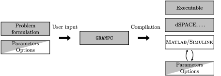
Figure 1: General structure of GRAMPC (grey: C code, white: Matlab level).

A specific problem can be parameterized and numerically solved using C/C++, Matlab/Simulink, or dSpace. A closer look on this functionality is given in Figure 2. The workspace of a GRAMPC project as well as algorithmic options and parameters are stored by the structure variable grampc. Several parameter settings are problem-specific and need to be provided, whereas other values are set to default values. A generic interface allows one to manipulate the grampc structure in order to set algorithmic options or parameters for the problem at hand. The functionalities of GRAMPC can be manipulated from Matlab/Simulink by means of mex routines that are wrappers for the corresponding C functions. This allow one to run a GRAMPC project with different parameters and options without recompilation.

4.2 Problem definition

The problem formulation in GRAMPC follows a generic structure. The essential steps for a problem definition are illustrated for the following MPC example

$$\min_{u(\cdot)} J(u;\boldsymbol{x}_{k})=\frac{1}{2}\Delta\boldsymbol{x}^{\mathsf{T}}(T)\boldsymbol{P}\Delta\boldsymbol{x}(T)+\frac{1}{2}\int_{0}^{T}\Delta\boldsymbol{x}^{\mathsf{T}}(T)\boldsymbol{Q}\Delta\boldsymbol{x}+R\Delta u^{2}\,{\rm d}\tau$$ (39a)

 s.t. $$\begin{bmatrix}\dot{x}_{1}\\ \dot{x}_{2}\end{bmatrix}=\begin{bmatrix}0&1\\ 0&0\end{bmatrix}\begin{bmatrix}x_{1}\\ x_{2}\end{bmatrix}+\begin{bmatrix}-0.04\\ -7.01\end{bmatrix}u\,,\quad\begin{bmatrix}x_{1}(0)\\ x_{2}(0)\end{bmatrix}=\begin{bmatrix}x_{k,1}\\ x_{k,2}\end{bmatrix}$$ (39b)

$$\begin{bmatrix}-0.2\\ -0.1\end{bmatrix}\leq\begin{bmatrix}x_{1}\\ x_{2}\end{bmatrix}\leq\begin{bmatrix}0.01\\ 0.1\end{bmatrix}\,,\quad|u|\leq 0.0524$$ (39c)

with $$\Delta\boldsymbol{x}=\boldsymbol{x}-\boldsymbol{x}_{\text{des}} \Delta u=u-u_{\text{des}}$$, , and the weights

$$\boldsymbol{P}=\boldsymbol{Q}=\begin{bmatrix}100&0\\ 0&10\end{bmatrix},\quad R=1\,.$$ (39d)

The dynamics (39b) are a simplified linear model of a single axis of a ball-on-plate system Richter2012 that is also included in the testbench of GRAMPC (see Section 5). The horizon length and the sampling time are set to $T=0.3$ s and $\Delta t=10\,$ms, respectively.

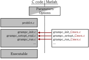
Figure 2: Interfacing of GRAMPC to C (grey) and Matlab (white). Each GRAMPC function written in plain C has a corresponding Cmex function.

The problem formulation (39) is provided in the user template probfct.c. The following listing gives an expression of the function structure and the problem implementation for the ball-on-plate example (39).

⬇

/* Problem dimensions */

void ocp_dim(typeInt *Nx, typeInt *Nu, typeInt *Np, typeInt *Ng, typeInt

*Nh, typeInt *NgT, typeInt *NhT, typeUSERPARAM *userparam)

{

*Nx = 2; *Nu = 1; *Np = 0;

*Nh = 4; *Ng = 0;

*NgT = 0; *NhT = 0;

}

/* Right-hand side of dynamics M dx/dt = f(t,x,u,p,userparam) */

void ffct(typeRNum *out, ctypeRNum t, ctypeRNum *x, ctypeRNum *u,

ctypeRNum *p, typeUSERPARAM *userparam)

{

out[0] = x[1]-0.04*u[0];

out[1] = -7.01*u[0];

}

/* Integral cost function int l(t,x(t),u(t),p,...) dt */

void lfct(typeRNum *out, ctypeRNum t, ctypeRNum *x, ctypeRNum *u, ctypeRNum

*p, ctypeRNum *xdes, ctypeRNum *udes, typeUSERPARAM *userparam)

{

typeRNum* param = (typeRNum*)userparam;

out[0] = 0.5*(param[0]*(x[0]-xdes[0])*(x[0]-xdes[0]) + \

param[1]*(x[1]-xdes[1])*(x[1]-xdes[1]) + \

param[2]*(u[0]-udes[0])*(u[0]-udes[0]) );

}

/* Terminal cost function V(T,x(T),p,xdes,userparam) */

void Vfct(typeRNum *out, ctypeRNum T, ctypeRNum *x, ctypeRNum *p,

ctypeRNum *xdes, typeUSERPARAM *userparam)

{

typeRNum* param = (typeRNum*)userparam;

out[0] = 0.5*(param[3]*(x[0]-xdes[0])*(x[0]-xdes[0]) + \

param[4]*(x[1]-xdes[1])*(x[1]-xdes[1]) );

}

/* Inequality constraints h(t,x(t),u(t),p,uperparam) <= 0 */

void hfct(typeRNum *out, ctypeRNum t, ctypeRNum *x, ctypeRNum *u,

ctypeRNum *p, typeUSERPARAM *userparam)

{

typeRNum* param = (typeRNum*)userparam;

out[0] = param[5] - x[0];

out[1] = -param[6] + x[0];

out[2] = param[7] - x[1];

out[3] = -param[8] + x[1];

}

The naming of the functions follows the nomenclature of the general OCP formulation (1), except for the function ocp_dim, which defines the dimensions of the optimization problem. Problem specific parameters can be used inside the single functions via the pointer userparam. For convenience, the desired setpoint (xdes,udes) to be stabilized by the MPC is provided to the cost functions separately and therefore does not need to be passed via userparam.

In addition to the single OCP functions, GRAMPC requires the derivatives w.r.t. state $\boldsymbol{x}$, control $\boldsymbol{u}$, and if applicable w.r.t. the optimization parameters $\boldsymbol{p}$ and end time $T$, in order to evaluate the optimality conditions in Algorithm 2. Jacobians that occur in multiplied form, see e.g. $(\frac{\partial\boldsymbol{f}}{\partial\boldsymbol{x}}\big{)}^{\mathsf{T}}\boldsymbol{\lambda}$ in the adjoint dynamics (22), have to be provided in this representation. This helps to avoid unnecessary zero multiplications in case of sparse Jacobians. The following listing shows an excerpt of the corresponding gradient functions.

⬇

/* Multiplied Jacobian (df/dx)^T * mult */

void dfdx_mult(typeRNum *out, ctypeRNum t, ctypeRNum *x, ctypeRNum *mult,

ctypeRNum *u, ctypeRNum *p, typeUSERPARAM *userparam)

{

out[0] = 0;

out[1] = mult[0];

}

...

/* Jacobian dl/dx */

void dldx(typeRNum *out, ctypeRNum t, ctypeRNum *x, ctypeRNum *u, ctypeRNum

*p, ctypeRNum *xdes, ctypeRNum *udes, typeUSERPARAM *userparam)

{

typeRNum* param = (typeRNum*)userparam;

out[0] = param[0]*(x[0]-xdes[0]);

out[1] = param[1]*(x[1]-xdes[1]);

}

...

/* Multiplied Jacobian (dh/dx)^T * mult */

void dhdx_mult(typeRNum *out, ctypeRNum t, ctypeRNum *x, ctypeRNum *u,

ctypeRNum *p, ctypeRNum *mult, typeUSERPARAM *userparam)

{

out[0] = -mult[0]+mult[1];

out[1] = -mult[2]+mult[3];

}

...

4.3 Calling procedure and options

GRAMPC provides several key functions that are required for initializing and calling the MPC solver. As shown in Figure 2, there exist mex wrapper functions that ensure that the interface for interacting with GRAMPC is largely the same under C/C++ and Matlab.

The following listing gives an idea on how to initialize GRAMPC and how to run a simple MPC loop for the ball-on-plate example under Matlab.

⬇

% user parameters

userparam = [100,10,1,100,10,-0.2,0.01,-0.1,0.1]

% initialization

grampc = grampc_init_Cmex(userparam);

% set parameters

grampc = grampc_setparam_Cmex(grampc,’x0’,[0.1;0.01]);

grampc = grampc_setparam_Cmex(grampc,’xdes’,[-0.2;0]);

grampc = grampc_setparam_Cmex(grampc,’u0’,0);

grampc = grampc_setparam_Cmex(grampc,’udes’,0);

grampc = grampc_setparam_Cmex(grampc,’Thor’,0.3);

grampc = grampc_setparam_Cmex(grampc,’dt’,0.01);

grampc = grampc_setparam_Cmex(grampc,’t0’,0);

grampc = grampc_setparam_Cmex(grampc,’umin’,0.0524);

grampc = grampc_setparam_Cmex(grampc,’umax’,-0.0524);

% set options

grampc = grampc_setopt_Cmex(grampc,’Nhor’,20);

grampc = grampc_setopt_Cmex(grampc,’MaxGradIter’,2);

grampc = grampc_setopt_Cmex(grampc,’MaxMultIter’,3);

grampc = grampc_setopt_Cmex(grampc,’InequalityConstraints’,’on’);

grampc = grampc_setopt_Cmex(grampc,’Integrator’,’heun’);

% MPC loop

for i = 1:iMPC

% run GRAMPC

grampc = grampc_run_Cmex(grampc);

...

% set new initial state

grampc = grampc_setparam_Cmex(grampc,’x0’,grampc.sol.xnext);

...

end

...

The listing also shows some of the algorithmic settings, e.g. the number of discretization points Nhor for the horizon $[0,T]$, the maximum number of iterations $(i_{\text{max}},j_{\text{max}})$ for Algorithm 1 and 2, or the choice of integration scheme for solving the canonical equations (22), (26). Currently implemented integration methods are (modified) Euler, Heun, 4th order Runge-Kutta as well as the solver RODAS Hairer:Book:1996:Stiff that implements a 4th order Rosenbrock method for solving semi-implicit differential-algebraic equations with possibly singular and sparse mass matrix $\boldsymbol{M}$, cf. the problem definition in (1). The Euler and Heun methods use a fixed step size depending on the number of discretization points (Nhor), whereas RODAS and Runge-Kutta use adaptive step size control. The choice of integrator therefore has significant impact on the computation time and allows one to optimize the algorithm in terms of accuracy and computational efficiency. Further options not shown in the listing are e.g. the settings (xScale, xOffset) and (uScale,uOffset) in order to scale the input and state variables of the optimization problem.

The initialization and calling procedure for GRAMPC is largely the same under C/C++ and Matlab. One exception is the handling of user parameters in userparam. Under C, userparam can be an arbitrary structure, whereas the Matlab interface restricts userparam to be of type array (of arbitrary length).

Moreover, the Matlab call of grampc_run_Cmex returns an updated copy of the grampc structure as output argument in order to comply with the Matlab policy to not manipulate input arguments.

5 Performance evaluation

The intention of this section is to evaluate the performance of GRAMPC under realistic conditions and for meaningful problem settings. To this end, an MPC testbench suite is defined to evaluate the computational performance in comparison to other state-of-the-art MPC solvers and to demonstrate the portability of GRAMPC to real-time and embedded hardware. The remainder of this section demonstrates the handling of typical problems from the field of MPC, moving horizon estimation and optimal control.

5.1 General MPC evaluation

The MPC performance of GRAMPC is evaluated for a testbench that covers a wide range of meaningful MPC applications. For the sake of comparison, the two MPC toolboxes ACADO and VIATOC are included in the evaluation, although it is not the intention of this section to rigorously rate the performance against other solvers, as such a comparison is difficult to carry out objectively. The evaluation should rather give a general impression about the performance and properties of GRAMPC. In addition, implementation details are presented for running the MPC testbench examples with GRAMPC on dSpace and ECU level.

5.1.1 Benchmarks

Table 1 gives an overview of the considered MPC benchmark problems in terms of the system dimension, the type of constraints (control/state/general nonlinear constraints), the dynamics (linear/nonlinear and explicit/semi-implicit) as well as the respective references. The MPC examples are evaluated with GRAMPC as well as with ACADO Toolkit Houska2011 and VIATOC Kalmari2015 .

The testbench includes three linear problems (mass-spring-damper, helicopter, ball-on-plate) and one semi-implicit reactor example, where the mass matrix $\boldsymbol{M}$ in the semi-implicit form (1b) is computed from the original partial differential equation (PDE) using finite elements, also see Section 5.2.3. The nonlinear chain problem is a scalable MPC benchmark with $m$ masses. Three further MPC examples are defined with nonlinear constraints. The permanent magnet synchronous machine (PMSM) possesses spherical voltage and current constraints in dq-coordinates, whereas the crane example with three degrees of freedom (DOF) and the vehicle problem include a nonlinear constraint to simulate a geometric restriction that must be bypassed (also see Section 5.2.1 for the crane example). Three of the problems (PMSM, 2D-crane, vehicle) are not evaluated with VIATOC, as nonlinear constraints cannot be handled by VIATOC at this stage.

Table 1: Overview of MPC benchmark problems.

Problem Dimensions Constraints Dynamics Reference $N_{\boldsymbol{x}}$ $N_{\boldsymbol{u}}$ $\boldsymbol{u}$ $\boldsymbol{x}$ nonl. semi-impl. linear Mass-spring-damper 10 2 yes no no no yes Kaepernick:diss:2016 Motor (PMSM) 4 2 yes yes yes no no Englert:CEP:2018 Nonl. chain ($m\!=\!4$) 21 3 yes no no no no Kirches2012 Nonl. chain ($m\!=\!6$) 33 3 yes no no no no Kirches2012 Nonl. chain ($m\!=\!8$) 45 3 yes no no no no Kirches2012 Nonl. chain ($m\!=\!10$) 57 3 yes no no no no Kirches2012 2D-Crane 6 2 yes yes yes no no Kaepernick2013 3D-Crane 10 3 yes no no no no Graichen2010 Helicopter 6 2 yes yes no no yes Tondel2002 Quadrotor 9 4 yes no no no no Kaepernick2014 VTOL 6 2 yes no no no no Sastry2013 Ball-on-plate 2 1 yes yes no no yes Richter2012 Vehicle 5 2 yes no yes no no Werling2012 CSTR reactor 4 2 yes no no no no Rothfuss1996 PDE reactor 11 1 yes no no yes no Utz2010

For the GRAMPC implementation, most options are set to their default values. The only adapted parameters concern the horizon length $T$, the number of supporting points for the integration scheme and the integrator itself as well as the number of augmented Lagrangian and gradient iterations, $i_{\text{max}}$ and $j_{\text{max}}$, respectively. Default settings are used for the multiplier and penalty updates for the sake of consistency, see Algorithm 1 as well as Section 3.5. Note, however, that the performance and computation time of GRAMPC can be further optimized by tuning the parameters related to the penalty update to a specific problem. All benchmark problems listed in Table 1 are available as example implementations in GRAMPC.

ACADO and VIATOC are individually tuned for each MPC problem by varying the number of shooting intervals and iterations in order to either achieve minimum computation time (setting “speed”) or optimal performance in terms of minimal cost at reasonable computational load (setting “optimal”). The solution of the quadratic programs of ACADO was done with qpOASES Ferreau:MPC:2014 .

The single MPC projects are integrated in a closed-loop simulation environment with a fourth-order Runge-Kutta integrator with adaptive step size to ensure an accurate system integration regardless of the integration schemes used internally by the MPC toolboxes. The evaluation was carried out on a Windows 10 machine with Intel(R) Core(TM) i5-5300U CPU running at $2.3\text{\,}\mathrm{GHz}$ using the Microsoft Visual C++ 2013 Professional (C) compiler. Each simulation was run multiple times to obtain a reliable average computation time.

5.1.2 Evaluation results

Table 2 shows the evaluation results for the benchmark problems in terms of computation time and cost value integrated over the whole time interval of the simulation scenario. The cost values are normalized to the best one of each benchmark problem. The results for ACADO and VIATOC are listed for the settings “speed” and “optimal”, as mentioned above. The depicted computation times are the mean computation times, averaged over the complete time horizon of the simulation scenario. The best values for computation time and performance (minimal cost) for each benchmark problem are highlighted in bold font.

The linear MPC problems (mass-spring-damper, helicopter, ball-on-plate) with quadratic cost functions can be tackled well by VIATOC and ACADO due to their underlying linearization techniques. The PDE reactor problem contains a stiff system dynamics in semi-implicit form. ACADO can handle such problems well using its efficient integration schemes, whereas VIATOC relies on fixed step size integrators and therefore requires a relatively large amount of discretization points. While GRAMPC achieves the fastest computation time, the cost value of both ACADO settings as well as the VIATOC optimal setting is lower. A similar cost function, however, can be achieved by GRAMPC when deviating from the default parameters.

In case of the state constrained 2D-crane problem, the overall cost is higher for ACADO than for GRAMPC. This appears to be due to the fact that almost over the complete simulation time a nonlinear constraint of a geometric object to be bypassed is active and ACADO does not reach the new setpoint in the given time. A closer look at this problem is taken in Section 5.2.1.

The CSTR reactor example possesses state and control variables in different orders of magnitude and therefore benefits from scaling. Since GRAMPC supports scaling natively, the computation time is faster than for VIATOC, where the scaling would have to be done manually. Due to the Hessian approximation used by ACADO, it is far less affected by the different scales in the states and controls.

A large difference in the cost values occurs for the VTOL example (Vertical Take-Off and Landing Aircraft). Due to the nonlinear dynamics and the corresponding coupling of the control variables, it seems that the gradient method underlying the minimization steps of GRAMPC is more accurate and robust when starting in an equilibrium position than the iterative linearization steps undertaken by ACADO and VIATOC.

Table 2: Evaluation results for the benchmark problems in Table 1 with overall integrated cost $J_{\text{int}}$ and computation time $t_{\text{CPU}}$ in milliseconds.

Problem GRAMPC ACADO ACADO VIATOC VIATOC (optimal) (speed) (optimal) (speed) $J_{\text{int}}$ $t_{\text{CPU}}$ $J_{\text{int}}$ $t_{\text{CPU}}$ $J_{\text{int}}$ $t_{\text{CPU}}$ $J_{\text{int}}$ $t_{\text{CPU}}$ $J_{\text{int}}$ $t_{\text{CPU}}$ Mass-spring-damper $\boldsymbol{1.000}$ $0.060$ $1.030$ $0.370$ $1.351$ $0.110$ $\boldsymbol{1.000}$ $0.075$ $1.221$ $\boldsymbol{0.049}$ Motor (PMSM) $1.006$ $\boldsymbol{0.032}$ $\boldsymbol{1.000}$ $0.129$ $1.096$ $0.057$ — — — — Nonl. chain ($m\!=\!4$) $1.003$ $2.022$ $1.003$ $4.666$ $1.027$ $\boldsymbol{1.770}$ $\boldsymbol{1.000}$ $12.32$ $1.041$ $7.660$ Nonl. chain ($m\!=\!6$) $\boldsymbol{1.000}$ $\boldsymbol{2.492}$ $\boldsymbol{1.000}$ $12.438$ $1.028$ $5.407$ $\boldsymbol{1.000}$ $18.10$ $1.042$ $11.48$ Nonl. chain ($m\!=\!8$) $\boldsymbol{1.000}$ $\boldsymbol{5.155}$ $1.005$ $26.834$ $1.050$ $10.127$ $\boldsymbol{1.000}$ $38.51$ $1.055$ $15.30$ Nonl. chain ($m\!=\!10$) $\boldsymbol{1.000}$ $\boldsymbol{7.810}$ $1.004$ $43.467$ $1.042$ $21.745$ $1.004$ $52.84$ $1.149$ $24.85$ 2D-Crane $\boldsymbol{1.000}$ $\boldsymbol{0.019}$ $1.932$ $0.446$ $2.110$ $0.058$ — — — — 3D-Crane ${1.002}$ $\boldsymbol{0.036}$ 1.000 $0.728$ $1.013$ $0.321$ $1.163$ $0.839$ $1.160$ $0.194$ Helicopter $1.017$ $0.054$ $1.006$ $0.163$ $1.096$ ${\boldsymbol{0.045}}$ $\boldsymbol{1.000}$ $0.185$ $1.060$ $0.071$ Quadrotor $\boldsymbol{1.000}$ $\boldsymbol{0.022}$ $\boldsymbol{1.000}$ $1.465$ $1.005$ $0.243$ $1.009$ $0.535$ $1.010$ $0.113$ VTOL $\boldsymbol{1.000}$ $\boldsymbol{0.033}$ $1.210$ $0.229$ $1.227$ $0.090$ $1.243$ $0.092$ $1.259$ $0.083$ Ball-on-plate $1.113$ $\boldsymbol{0.014}$ $1.112$ $0.068$ $1.126$ $0.022$ $\boldsymbol{1.000}$ $0.116$ $1.158$ $0.018$ Vehicle $1.027$ $\boldsymbol{0.092}$ $\boldsymbol{1.000}$ $1.313$ $1.003$ $0.322$ — — — — CSTR reactor $\boldsymbol{1.000}$ $\boldsymbol{0.058}$ $\boldsymbol{1.000}$ $0.195$ $1.002$ $0.076$ $1.016$ $3.711$ $1.532$ $0.176$ PDE reactor $1.059$ $\boldsymbol{0.362}$ $\boldsymbol{1.000}$ $6.259$ $1.005$ $0.498$ $1.046$ $7.214$ $1.072$ $2.868$

The scaling behavior of the MPC schemes w.r.t. the problem dimension is investigated for the nonlinear chain in Table 2. Four different numbers of masses are considered, corresponding to 21-57 state variables and three controls. Although the algorithmic complexity of the augmented Lagrangian/gradient projection algorithm of GRAMPC grows linearly with the state dimension, this is not exactly the case for the nonlinear chain, as the stiffness of the dynamics increases for a larger number of masses, which leads to smaller step sizes of the adaptive Runge-Kutta integrator that was used in GRAMPC for this problem. ACADO shows a more significant increase in computation time for larger values of $m$, which was to be expected in view of the SQP algorithm underlying ACADO. The computation time for VIATOC is worse for this example, since only fixed step size integrators are available in the current release, which requires to increase the number of discretization points manually. Figure 3 shows a logarithmic plot of the computation time for all three MPC solvers plotted over the number of masses of the nonlinear chain.

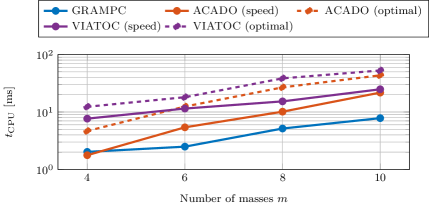
Figure 3: Computation time for the nonlinear chain example (also see Table 2).

The computation times shown in Table 2 are average values and therefore give no direct insight into the real-time feasibility of the MPC solvers and the variation of the computational load over the single sampling steps. To this end, Figure 4 shows accumulation plots of the computation time per MPC step for three selected problems of the testbench. The computation times were evaluated after 30 successive runs to obtain reliable results. The plots show that the computation time of GRAMPC is almost constant for each MPC iteration, which is important for embedded control applications and to give tight upper bounds on the computation time for real-time guarantees. ACADO and VIATOC show a larger variation of the computation time over the iterations, which is mainly due to the active set strategy that both solvers follow and the varying number of QP iterations in each real-time iteration of ACADO, c.f. Houska2011 .

In conclusion, it can be said that GRAMPC has overall fast and real-time feasible computation times for all benchmark problems, in particular for nonlinear systems and in connection with (nonlinear) constraints. Furthermore, GRAMPC scales well with increasing system dimension.

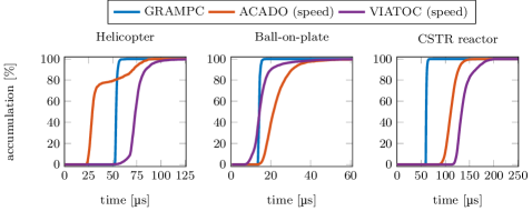
Figure 4: Accumulation of the computation times for three different examples (averaged over 30 runs).

5.1.3 Embedded realization

Table 3: Computation time and memory usage for the embedded realization of GRAMPC on dSpace hardware (DS1202) and ECU level (Renesas RH850/P1M) with single floating point precision.

Problem $t_{\text{{\rm{d}Space}}}$ $t_{\text{ECU}}$ Memory Problem $t_{\text{{\rm{d}Space}}}$ $t_{\text{ECU}}$ Memory Mass-spring-damper $0.24\text{\,}\mathrm{ms}$ $4.00\text{\,}\mathrm{ms}$ $6.5\text{\,}\mathrm{kB}$ Helicopter $0.11\text{\,}\mathrm{ms}$ $1.88\text{\,}\mathrm{ms}$ $5.8\text{\,}\mathrm{kB}$ Motor (PMSM) $0.13\text{\,}\mathrm{ms}$ $2.10\text{\,}\mathrm{ms}$ $2.4\text{\,}\mathrm{kB}$ Quadrotor $0.21\text{\,}\mathrm{ms}$ $1.60\text{\,}\mathrm{ms}$ $4.4\text{\,}\mathrm{kB}$ Nonl. chain ($m\!=\!4$) $4.79\text{\,}\mathrm{ms}$ $-$ $12.9\text{\,}\mathrm{kB}$ VTOL $0.37\text{\,}\mathrm{ms}$ $2.80\text{\,}\mathrm{ms}$ $6.2\text{\,}\mathrm{kB}$ Nonl. chain ($m\!=\!6$) $9.62\text{\,}\mathrm{ms}$ $-$ $18.5\text{\,}\mathrm{kB}$ Ball-on-plate $0.05\text{\,}\mathrm{ms}$ $0.92\text{\,}\mathrm{ms}$ $2.0\text{\,}\mathrm{kB}$ Nonl. chain ($m\!=\!8$) $17.50\text{\,}\mathrm{ms}$ $-$ $24.1\text{\,}\mathrm{kB}$ Vehicle $0.25\text{\,}\mathrm{ms}$ $2.69\text{\,}\mathrm{ms}$ $3.6\text{\,}\mathrm{kB}$ Nonl. chain ($m\!=\!10$) $24.20\text{\,}\mathrm{ms}$ $-$ $29.8\text{\,}\mathrm{kB}$ CSTR reactor $0.43\text{\,}\mathrm{ms}$ $6.81\text{\,}\mathrm{ms}$ $5.1\text{\,}\mathrm{kB}$ 2D-Crane $0.18\text{\,}\mathrm{ms}$ $1.65\text{\,}\mathrm{ms}$ $4.5\text{\,}\mathrm{kB}$ PDE reactor $6.48\text{\,}\mathrm{ms}$ $-$ $15.0\text{\,}\mathrm{kB}$ 3D-Crane $0.31\text{\,}\mathrm{ms}$ $3.05\text{\,}\mathrm{ms}$ $7.3\text{\,}\mathrm{kB}$

In addition to the general MPC evaluation, this section evaluates the computation time and memory requirements of GRAMPC for the benchmark problems on real-time and embedded hardware. GRAMPC was implemented on a dSpace MicroLabbox (DS1202) with a $2\text{\,}\mathrm{GHz}$ Freescale QolQ processor as well as on the microntroller RH850/P1M from Renesas with a CPU frequency of $160\text{\,}\mathrm{MHz}$, $2\text{\,}\mathrm{MB}$ program flash and $128\text{\,}\mathrm{kB}$ RAM. This processor is typically used in electronic control units (ECU) in the automotive industry. The GRAMPC implementation on this microcontroller therefore can be seen as a prototypical ECU realization. As it is commonly done in embedded systems, GRAMPC was implemented using single floating point precision on both systems due to the floating point units of the processors.

Table 3 lists the computation time and RAM memory footprint of GRAMPC on both hardware platforms for the testbench problems in Table 1 and 2. The settings of GRAMPC are the same as in the previous section, except for the floating point precision. Due to the compilation size limit of the ECU compiler ($<10$ kB), the nonlinear chain examples as well as the PDE reactor could not be compiled on the ECU.

The computation times on the dSpace hardware are below the sampling time for all example problems. The same holds for the ECU implementation, except for the 2D-crane, the PMSM, and the VTOL example. However, as mentioned before, tuning of the algorithm can further reduce the runtime, as most of the multiplier and penalty update parameters are taken as default. Note that there is no constant scaling factor between the computation times on dSpace and ECU level, which is probably due to the different realization of the math functions by the respective floating point unit / compiler on the different hardware.

The required memory is below $9\text{\,}\mathrm{kB}$ for all examples, except for the nonlinear chain and the PDE reactor, which is less than $7\text{\,}\mathrm{\char 37\relax}$ of the available RAM on the considered ECU. Although the nonlinear chain and the PDE reactor could not be compiled on the ECU as mentioned above, the memory usage as well as the computation time increase only linearly with the size of the system (using the same GRAMPC settings). Overall, the computational speed and the small memory footprint demonstrate the applicability of GRAMPC for embedded systems.

5.2 Application examples

This section discusses some application examples, including a more detailed view on two selected problems from the testbench collection (state constrained and semi-implicit problem), a shrinking horizon MPC application, an equality constrained OCP as well as a moving horizon estimation problem.

5.2.1 Nonlinear constrained model predictive control

The 2D-crane example in Table 1 and 2 is a particularly challenging one, as it is subject to a nonlinear constraint that models the collision avoidance of an object or obstacle. A schematic representation of the overhead crane is given in Figure 5. The crane has three degrees-of-freedom and the nonlinear dynamics read as Kaepernick2013

$$\ddot{s}_{\text{C}}=u_{1},\quad\ddot{s}_{\text{R}}=u_{2},\quad\ddot{\phi}=-\frac{1}{s_{\text{R}}}\left(g\sin(\phi)+a_{\text{C}}\cos(\phi)+2\dot{s}_{\text{R}}\dot{\phi}\right)$$

with the gravitational constant $g$. The system state $\boldsymbol{x}=[s_{\text{C}},\dot{s}_{\text{C}},s_{\text{R}},\dot{s}_{\text{R}},\phi,\dot{\phi}]^{\mathsf{T}}\in\mathbb{R}^{6}$ comprises the cart position $s_{\text{C}}$, the rope length $s_{\text{R}}$, the angular deflection $\phi$ and the corresponding velocities. The two controls $\boldsymbol{u}\in\mathbb{R}^{2}$ are the cart acceleration $u_{1}$ and the rope acceleration $u_{2}$, respectively.

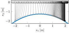
Figure 5: Schematic representation of the overhead crane (left) and simulated crane movement from the initial state to the desired setpoint (right).

The cost functional (2a) consists of the integral part

$$l(\boldsymbol{x},\boldsymbol{u})=(\boldsymbol{x}-\boldsymbol{x}_{\text{des}})^{\mathsf{T}}\boldsymbol{Q}(\boldsymbol{x}-\boldsymbol{x}_{\text{des}})+(\boldsymbol{u}-\boldsymbol{u}_{\text{des}})^{\mathsf{T}}\boldsymbol{R}(\boldsymbol{u}-\boldsymbol{u}_{\text{des}})\,,$$ (40)

which penalizes the deviation from the desired setpoints $\boldsymbol{x}_{\mathrm{des}}\in\mathbb{R}^{6}$ and $\boldsymbol{u}_{\mathrm{des}}\in\mathbb{R}^{2}$ respectively. The weight matrices are set to $\boldsymbol{Q}={\rm diag}(1,2,2,1,1,4)$ and $\boldsymbol{R}={\rm diag}(0.05,0.05)$ (omitting units). The controls and angular velocity are subject to the box constraints $|u_{i}|\leq$2\text{\,}\mathrm{m}\text{\,}{\mathrm{s}}^{-2}$,\,i\in{1,2}$ and $|\dot{\phi}|\leq$0.3\text{\,}\mathrm{rad}\text{\,}{\mathrm{s}}^{-1}$,\,i\in{1,2}$. In addition, the nonlinear inequality constraint

$$h(\boldsymbol{x})=\cos(\phi)s_{\text{R}}-$0.2\text{\,}{\mathrm{m}}^{-1}$\left(s_{\text{C}}+\sin(\phi)s_{\text{R}}\right)^{2}+$1.25\text{\,}\mathrm{m}$\leq 0$$ (41)

is imposed, which represents a geometric security constraint, e.g. for trucks, over which the load has to be lifted, see Figure 6 (right).

The prediction horizon and sampling time for the crane problem are set to $T=$2\text{\,}\mathrm{s}$$ and $\Delta t=$2\text{\,}\mathrm{ms}$$, respectively. The number of augmented Lagrangian steps and inner gradient iterations of GRAMPC are set to $(i_{\text{max}},j_{\text{max}})=(1,2)$. These settings correspond to the computational results in Table 2 and 3.

The right part of Figure 5 illustrates the movement of the overhead crane from the initial state $\boldsymbol{x}_{0}=\left[$-2\text{\,}\mathrm{m}$,0,$2\text{\,}\mathrm{m}$,0,0,0\right]^{\mathsf{T}}$ to the desired setpoint $\boldsymbol{x}_{\text{des}}=\left[$2\text{\,}\mathrm{m}$,0,$2\text{\,}\mathrm{m}$,0,0,0\right]^{\mathsf{T}}$. Figure 6 shows the corresponding trajectories of the states $\boldsymbol{x}(t)$ and controls $\boldsymbol{u}(t)$ as well as the nonlinear constraint (41) plotted as time function $h(\boldsymbol{x}(t))$. This transition problem is quite challenging, since the nonlinear constraint (41) is active for more than half of the simulation time. One can slightly see an initial violation of the constraint $h(\boldsymbol{x})$ of approximately $1\text{\,}\mathrm{mm}$, which should be negligible in practical applications. Nevertheless, one can satisfy the constraint to a higher accuracy by increasing the number of iterations $(i_{\text{max}},j_{\text{max}})$, in particular of the augmented Lagrangian iterations.

5.2.2 MPC on shrinking horizon

“Classical” MPC with a constant horizon length typically acts as an asymptotic controller in the sense that a desired setpoint is only reached asymptotically. MPC on a shrinking horizon instead reduces the horizon time $T$ in each sampling step in order to reach the desired setpoint in finite time. In particular, if the desired setpoint is incorporated into a terminal constraint and the prediction horizon $T$ is optimized in each MPC step, then $T$ will be automatically reduced over the runtime due to the principle of optimality.

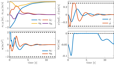
Figure 6: MPC trajectories for the 3DOF crane.

Shrinking horizon MPC with GRAMPC is illustrated for the following double integrator problem

$$\min_{u,T} J(u,T;\boldsymbol{x}_{k})=T+\frac{1}{2}\int_{0}^{T}ru^{2}(\tau)\,{\rm d}\tau$$ (42a)

 s.t. $$\dot{x}_{1}(\tau)=x_{2}(\tau)\,,\quad x_{1}(0)=x_{1,k}=x_{1}(t_{k})$$ (42b)

$$\dot{x}_{2}(\tau)=u(\tau)\,,\quad x_{2}(0)=x_{2,k}=x_{2}(t_{k})$$ (42c)

$$|u(\tau)|\leq 1\,,\quad \tau\in[0,T]$$ (42d)

$$\boldsymbol{x}(T)=\boldsymbol{x}_{\text{des}}$$ (42e)

with the state $\boldsymbol{x}=[x_{1},x_{2}]^{\mathsf{T}}$ and control $u$ subject to the box constraint (42d). The weight $r>0$ in the cost functional (42a) allows a trade-off between energy optimality and time optimality of the MPC. The desired setpoint $\boldsymbol{x}_{\text{des}}$ is added as terminal constraint (42e), i.e. $\boldsymbol{g}_{T}(\boldsymbol{x}(T)):=\boldsymbol{x}(T)-\boldsymbol{x}_{\text{des}}=\boldsymbol{0}$ in view of (1c), and the prediction horizon $T$ is treated as optimization variable in addition to the control $u(\tau)$, $\tau\in[0,T]$.

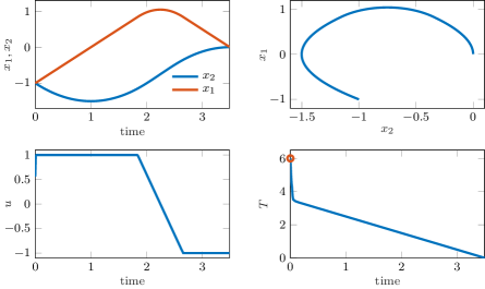
Figure 7: MPC trajectories with shrinking horizon for the double integrator problem (42).

For the simulations, the weight in the cost functional is set to $r=0.01$ and the initial value of the horizon length is chosen as $T=6$. The iteration numbers for GRAMPC are set to $(i_{\text{max}},j_{\text{max}})=(1,2)$ in conjunction with a sampling time of $\Delta t=0.001$ in order to resemble a real-time implementation. Figure 7 shows the simulation results for the double integrator problem with the desired setpoint $\boldsymbol{x}_{\text{des}}=\boldsymbol{0}$ and the initial state $\boldsymbol{x}(0)=[-1,-1]^{\mathsf{T}}$. Obviously, the state trajectories reach the origin in finite time corresponding to the anticipated behavior of the shrinking horizon MPC scheme. The lower right plot of Figure 7 shows the temporal evolution of the horizon length $T$ over the runtime $t$. The initial end time of $T=6$ is marked as a red circle. In the first MPC steps, the optimization quickly decreases the end time to approximately $T=3.5$. In this short time interval, GRAMPC produces a suboptimal solution due to the strict limitation of the iterations $(i_{\text{max}},j_{\text{max}})$. Afterwards, however, the prediction horizon declines linearly, which concurs with the principle of optimality and shows the optimality of the computed trajectories after the initialization phase. In the simulated example, this knowledge is incorporated in the MPC implementation by substracting the sampling time $\Delta t$ from the last solution of $T$ for warm-starting the next MPC step. The simulation is stopped as soon as the horizon length reaches its minimum value $T_{\mathrm{min}}=\Delta t=0.1$.

5.2.3 Semi-implicit problems

The system formulations that can be handled with GRAMPC include DAE systems with singular mass matrix $\boldsymbol{M}$ as well as general semi-implicit systems. An application example is the discretization of spatially distributed systems by means of finite elements. This is illustrated for a quasi-linear diffusion-convection-reaction system, which is also implemented in the testbench (PDE reactor example). The thermal behavior of the reactor is described on the one-dimensional spatial domain $z=(0,1)$ using the PDE formulation Utz2010

$$\partial_{t}\theta=\partial_{z}\left[(q_{0}+q_{1}\theta)\partial_{z}\theta-\nu\theta\right]+(r_{0}+r_{1}\theta)\theta$$ (43a)

with the boundary and initial conditions

$$\partial_{z}\theta|_{z=0} =0$$ (43b)

$$\partial_{z}\theta|_{z=1}+\theta(1,t) =u$$ (43c)

$$\theta(\cdot,0) =\theta_{0}$$ (43d)

for the temperature $\theta=\theta(z,t)$. The process is controlled by the boundary control $u=u(t)$. Diffusive and convective processes of the reactor are modeled by the nonlinear heat equation (43a) with the parameters $q_{1}=$2$$, $q_{2}=$-0.05$$, and $\nu=$1$$, respectively. Reaction effects are included using the parameters $r_{0}=$1$$ and $r_{1}=$0.2$$. The Neumann boundary condition (43b), the Robin boundary condition (43c), and the initial condition (43) complete the mathematical description of the system dynamics. Both spatial and time domain are normalized for the sake of simplicity. A more detailed description of the system dynamics can be found in Utz2010 .

The PDE system (43) is approximated by an ODE system of the form (20a) by applying a finite element discretization technique zienkiewicz_book1983_fem , whereby the new state variables $\boldsymbol{x}\in\mathbb{R}^{N_{\boldsymbol{x}}}$ approximate the temperature $\theta$ on the discretized spatial domain $z$ with $N_{\boldsymbol{x}}$ spatial grid points. The finite element discretization eventually leads to a finite-dimensional system dynamics of the form $\boldsymbol{M}\boldsymbol{\dot{x}}=\boldsymbol{f}(\boldsymbol{x},u)$ with the mass matrix $\boldsymbol{M}\in\mathbb{R}^{N_{\boldsymbol{x}}\times N_{\boldsymbol{x}}}$ and the nonlinear system function $\boldsymbol{f}(\boldsymbol{x},u)$. In particular, $N_{\boldsymbol{x}}=11$ grid points are chosen for the GRAMPC simulation of the reactor (43). The upper right plot of Figure 8 shows the sparsity structure of the mass matrix $\boldsymbol{M}\in\mathbb{R}^{11\times 11}$.

The control task for the reactor is the stabilization of a stationary profile $\boldsymbol{x}_{\text{des}}$ which is accounted for in the quadratic MPC cost functional

$$J(u;\boldsymbol{x}_{k}):=\tfrac{1}{2}\big{\|}\boldsymbol{x}(T)-\boldsymbol{x}_{\rm des}\big{\|}^{2}+\int_{0}^{T}\tfrac{1}{2}\big{\|}\boldsymbol{x}(t)-\boldsymbol{x}_{\rm des}\big{\|}^{2}+${10}^{-2}$\big{\|}u-u_{\rm des}\big{\|}^{2}\,{\rm d}t\,.$$

The desired setpoint $(\boldsymbol{x}_{\text{des}},u_{\text{des}})$ as well as the initial values $(\boldsymbol{x}_{0},u_{0})$ are numerically determined from the stationary differential equation

$$0 =\partial_{z}\left[(q_{0}+q_{1}\theta(z,\tau))\partial_{z}\theta(z,\tau)-\nu\theta(z,\tau)\right]+(r_{0}+r_{1}\theta(z,\tau))\theta(z,\tau)$$ (44)

with the corresponding boundary conditions

$$\theta(0,0) =1, \quad\partial_{z}\theta(0,0) =0$$

$$\theta(0,\infty) =2, \quad\partial_{z}\theta(0,\infty) =0\,.$$

The prediction horizon and sampling time of the MPC scheme are set to $T=$0.2$$ and $\Delta t=$0.005$$. The number of iterations are limited by $(i_{\text{max}},j_{\text{max}})=(1,2)$. The box constraints for the control are chosen as $|u(t)|\leq 2$.

The numerical integration in GRAMPC is carried out using the solver RODAS Hairer:Book:1996:Stiff . The sparse numerics of RODAS allow one to cope with the banded structure of the matrices in a computationally efficient manner. Figure 8 shows the setpoint transition from the initial temperature profile $\boldsymbol{x}_{0}$ to the desired temperature $\boldsymbol{x}_{\rm des}=[2.00,1.99,1.97,1.93,1.88,1.81,1.73,1.63,1.51,1.38,1.23]^{\mathsf{T}}$ and desired control $u_{\text{des}}=-1.57$.

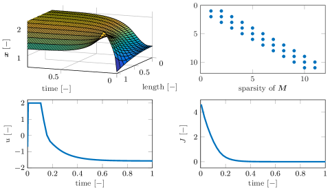
Figure 8: Simulated MPC trajectories for the PDE reactor (43).

5.2.4 OCP with equality constraints

An illustrative example of an optimal control problem with equality constraints is a dual arm robot with closed kinematics, e.g. to handle or carry work pieces with both arms. For simplicity, a planar dual arm robot with the joint angles $(x_{1},x_{2},x_{3})$ and $(x_{4},x_{5},x_{6})$ for the left and right arm is considered. The dynamics are given by simple integrators

$$\boldsymbol{\dot{x}}=\begin{bmatrix}\dot{x}_{1}&\dot{x}_{2}&\dot{x}_{3}&\dot{x}_{4}&\dot{x}_{5}&\dot{x}_{6}\end{bmatrix}^{\mathsf{T}}=\begin{bmatrix}u_{1}&u_{2}&u_{3}&u_{4}&u_{5}&u_{6}\end{bmatrix}^{\mathsf{T}}=\boldsymbol{u}$$ (45)

with the joint velocities as control input $\boldsymbol{u}$. Given the link lengths $\boldsymbol{a}=[a_{1}$, $a_{2}$, $a_{3}$, $a_{4}$, $a_{5}$, $a_{6}]$, the forward kinematics of left and right arm are computed by

$$\boldsymbol{p}_{\mathrm{L}}(\boldsymbol{x})=\begin{bmatrix}a_{1}\cos(x_{1})+a_{2}\cos(x_{1}+x_{2})+a_{3}\cos(x_{1}+x_{2}+x_{3})\\ a_{1}\sin(x_{1})+a_{2}\sin(x_{1}+x_{2})+a_{3}\sin(x_{1}+x_{2}+x_{3})\\ x_{1}+x_{2}+x_{3}\end{bmatrix}$$ (46)

and

$$\boldsymbol{p}_{\mathrm{R}}(\boldsymbol{x})=\begin{bmatrix}1+a_{4}\cos(x_{4})+a_{5}\cos(x_{4}+x_{5})+a_{6}\cos(x_{4}+x_{5}+x_{6})\\ a_{4}\sin(x_{4})+a_{5}\sin(x_{4}+x_{5})+a_{6}\sin(x_{4}+x_{5}+x_{6})\\ x_{4}+x_{5}+x_{6}\end{bmatrix}\,.$$ (47)

The closed kinematic chain is enforced by the equality constraint

$$\boldsymbol{g}(\boldsymbol{x}):=\boldsymbol{p}_{\mathrm{L}}(\boldsymbol{x})-\boldsymbol{p}_{\mathrm{R}}(\boldsymbol{x})-\left[0,\,0,\,\pi\right]^{\mathsf{T}}=\boldsymbol{0}\,.$$ (48)

A point-to-point motion from $\boldsymbol{x}_{0}=[\frac{\pi}{2},-\frac{\pi}{2},0,-\frac{\pi}{2},\frac{\pi}{2},0]^{\mathsf{T}}$ to $\boldsymbol{x}_{f}=[-\frac{\pi}{2}$, $\frac{\pi}{2}$, $0$, $\frac{\pi}{2}$, $-\frac{\pi}{2}]^{\mathsf{T}}$ is considered as control task, which is formulated as the optimal control problem

$$\min_{\boldsymbol{u}}\quad J(\boldsymbol{u}):=\int_{0}^{T}\frac{1}{2}\boldsymbol{u}(t)^{\mathsf{T}}\boldsymbol{R}\boldsymbol{u}(t)\,{\rm d}t$$ (49a)

s.t. $$\boldsymbol{\dot{x}}(t)=\boldsymbol{u}(t)\,,\quad \boldsymbol{x}(0)=\boldsymbol{x}_{0}\,,\quad\boldsymbol{x}(T)=\boldsymbol{x}_{f}$$ (49b)

$$\boldsymbol{g}(\boldsymbol{x}(t))=\boldsymbol{0}\,,\quad \boldsymbol{u}(t)\in\left[\boldsymbol{u}_{\text{min}},\boldsymbol{u}_{\text{max}}\right]$$ (49c)

with the fixed end time $T=10\,\text{s}$ and the control constraints $-\boldsymbol{u}_{\text{min}}=\boldsymbol{u}_{\text{max}}=[1,1,1,1,1,1]^{\mathsf{T}}\text{s}^{-1}$, which limit the angular speeds of the robot arms. The cost functional minimizes the squared joint velocities with $\boldsymbol{R}=\boldsymbol{I}_{\!6}$.

Table 4: Computation results for the planar two-arm robot with closed kinematics.

Gradient Constraint Gradient iter- Augm. Lagr. $t_{\text{CPU}}$ tol. $\varepsilon_{\text{rel,c}}$ tol. $\boldsymbol{\varepsilon}_{\boldsymbol{g}}$ ations $i$ (avg.) iterations $j$ [ms] $1\text{\times}{10}^{-5}$ $1\text{\times}{10}^{-3}$ 64 189 $135$ $1\text{\times}{10}^{-6}$ $1\text{\times}{10}^{-4}$ 65 298 $214$ $1\text{\times}{10}^{-7}$ $1\text{\times}{10}^{-5}$ 306 190 $628$ $1\text{\times}{10}^{-8}$ $1\text{\times}{10}^{-6}$ 222 431 $1015$

Table 4 shows the computation results of GRAMPC for solving OCP (49) with increasingly restrictive values of the gradient tolerance $\varepsilon_{\text{rel,c}}$ and constraint tolerance $\boldsymbol{\varepsilon}_{\boldsymbol{g}}$ that are used for checking convergence of Algorithm 1 and 2. The required computation time $t_{\text{CPU}}$ as well as the average number of (inner) gradient iterations and the number of (outer) augmented Lagrangian iterations are shown in Table 4. The successive reduction of the tolerances $\varepsilon_{\text{rel,c}}$ and $\boldsymbol{\varepsilon}_{\boldsymbol{g}}$ highlights that the augmented Lagrangian framework is able to quickly compute a solution with moderate accuracy. When further tightening the tolerances, the computation time as well as the required iterations increase clearly. This is to be expected as augmented Lagrangian and gradient algorithms are linearly convergent opposed to super-linear or quadratic convergence of, e.g., SQP or interior point methods. However, as the main application of GRAMPC is model predictive control, the ability to quickly compute suboptimal solutions that are improved over time is more important than the numerical solution for very small tolerances.

The resulting trajectory of the planar robot is depicted in Figure 9 and shows that the solution of the optimal control problem (49) involves moving through singular configurations of left and right arm, which makes this problem quite challenging.

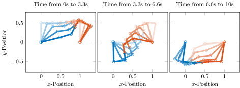
Figure 9: Solution trajectory for the planar two-arm robot with closed kinematics.

5.2.5 Moving horizon estimation

Another application domain for GRAMPC is moving horizon estimation (MHE) by taking advantage of the parameter optimization functionality. This is illustrated for the CSTR reactor model listed in the MPC testbench in Table 1. The system dynamics of the reactor is given by Rothfuss1996

$$\dot{c}_{\mathrm{A}} =-k_{1}(T)c_{\mathrm{A}}-k_{2}(T)c_{\mathrm{A}}^{2}+(c_{\mathrm{in}}-c_{\mathrm{A}})u_{1}$$ (50a)

$$\dot{c}_{\mathrm{B}} =k_{1}(T)c_{\mathrm{A}}-k_{1}(T)c_{\mathrm{B}}-c_{\mathrm{B}}u_{1}$$ (50b)

$$\dot{T}~{} =-\delta(k_{1}(T)c_{\mathrm{A}}\Delta H_{\mathrm{AB}}+k_{1}(T)\Delta H_{\mathrm{BC}}+k_{2}(T)c_{\mathrm{A}}^{2}\Delta H_{\mathrm{AD}})$$

$$\hskip 28.45274pt+\alpha(T_{\mathrm{C}}-T)+(T_{\mathrm{in}}-T)u_{1}$$ (50c)

$$\dot{T}_{\mathrm{C}} =\beta(T-T_{\mathrm{C}})+\gamma u_{2}$$ (50d)

with the state vector $\boldsymbol{x}=[c_{\mathrm{A}},c_{\mathrm{B}},T,T_{\mathrm{C}}]^{\mathsf{T}}$ consisting of the monomer and product concentrations $c_{\mathrm{A}}$, $c_{\mathrm{B}}$ and the reactor and cooling temperature $T$ and $T_{\mathrm{C}}$. The control variables $\boldsymbol{u}=[u_{1},u_{2}]^{\mathsf{T}}$ are the normalized flow rate and cooling power. The measured quantities are the temperatures $y_{1}=T$ and $y_{2}=T_{\mathrm{C}}$. The parameter values and a more detailed description of the system are given in Rothfuss1996 .

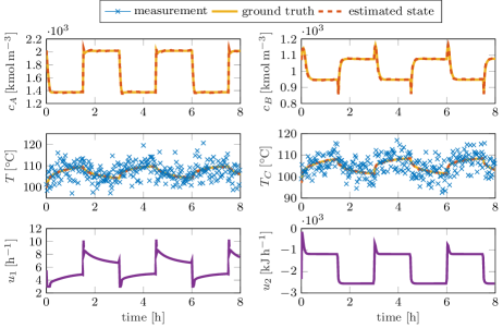
Figure 10: MHE/MPC simulation results for the CSTR reactor.

The following scenario considers the interconnection of the MHE with the MPC from the testbench, i.e. the state $\boldsymbol{\hat{x}}_{k}$ at the sampling time $t_{k}$ is estimated and provided to the MPC. The cost functional of the MPC is designed according to

$$J(\boldsymbol{u};\boldsymbol{x}_{k}):=\Delta\boldsymbol{x}^{\mathrm{T}}(T)\boldsymbol{P}\Delta\boldsymbol{x}(T)+\int_{0}^{T}\Delta\boldsymbol{x}^{\mathrm{T}}(t)\boldsymbol{Q}\Delta\boldsymbol{x}(t)+\Delta\boldsymbol{u}^{\mathrm{T}}(t)\boldsymbol{R}\Delta\boldsymbol{u}(t)\,{\rm d}t\,,$$ (51)

where $\Delta\boldsymbol{x}=\boldsymbol{x}-\boldsymbol{x}_{\mathrm{des}}$ and $\Delta\boldsymbol{u}=\boldsymbol{u}-\boldsymbol{u}_{\mathrm{des}}$ penalize the deviation of the state and control from the desired setpoint $(\boldsymbol{x}_{\mathrm{des}},\boldsymbol{u}_{\mathrm{des}})$. The MHE uses the cost functional defined in Section 2.3, c.f. (5a). The sampling rate for both MPC and MHE is set to $\Delta t=$1\text{\,}\mathrm{s}$$. The MPC runs with a prediction horizon of $T=$20\text{\,}\mathrm{min}$$ and $40$ discretization points, while the MHE horizon is set to $T_{\mathrm{MHE}}=$10\text{\,}\mathrm{s}$$ with $10$ discretization points. The GRAMPC implementation of the MHE uses only one gradient iteration per sampling step, i.e. $(i_{\text{max}},j_{\text{max}})=(1,1)$, while the implementation of the MPC uses three gradient iterations, i.e. $(i_{\text{max}},j_{\text{max}})=(1,3)$.

The simulated scenario in Figure 10 consists of alternating setpoint changes between two stationary points. The two measured temperatures are subject to a Gaussian measurement noise with a standard deviation of $4\text{\,}\mathrm{\SIUnitSymbolCelsius}$. The initial guess for the state vector $\boldsymbol{x}$ of the MHE differs from the true initial values by $100\text{\,}\mathrm{kmol}\text{\,}{\mathrm{m}}^{-3}$ for both concentrations $c_{\text{A}}$ and $c_{\text{B}}$ and by $5\text{\,}\mathrm{\SIUnitSymbolCelsius}$, respectively $-7\text{\,}\mathrm{\SIUnitSymbolCelsius}$, for the reactor and cooling temperature. This initial disturbance vanishes within a few iterations and the MHE tracks the ground truth (i.e. the simulated state values) closely, with an average error of $\delta\boldsymbol{\hat{x}}=[$7.12\text{\,}\mathrm{kmol}\text{\,}{\mathrm{m}}^{-3}$$, $6.24\text{\,}\mathrm{kmol}\text{\,}{\mathrm{m}}^{-3}$, $0.10\text{\,}\mathrm{\SIUnitSymbolCelsius}$, $$0.09\text{\,}\mathrm{\SIUnitSymbolCelsius}$]^{\mathsf{T}}$. This corresponds to a relative error of less than $0.1\text{\,}\mathrm{\char 37\relax}$ for each state variable, when normalized to the respective maximum value. One iteration of the MHE requires a computation time of $t_{\mathrm{CPU}}=$11\text{\,}\mathrm{\SIUnitSymbolMicro s}$$ to calculate a new estimate of the state vector $\boldsymbol{x}$ and therefore about one third of the time necessary for one MPC iteration.

6 Conclusions

The augmented Lagrangian algorithm presented in this paper is implemented in the nonlinear model predictive control (MPC) toolbox GRAMPC and extends its original version that was published in 2014 in several significant aspects. The system class that can be handled by GRAMPC are general nonlinear systems described by explicit or semi-implicit differential equations or differential-algebraic equations (DAE) of index 1. Besides input constraints, the algorithm accounts for nonlinear state and/or input dependent equality and inequality constraints as well as for unknown parameters and a possibly free end time as further optimization variables, which is relevant, for instance, for moving horizon estimation or MPC on a shrinking horizon. The computational efficiency of GRAMPC is illustrated for a testbench of representative MPC problems and in comparison with two state-of-the-art nonlinear MPC toolboxes. In particular, the augmented Lagrangian algorithm implemented in GRAMPC is tailored to embedded MPC with very low memory requirements. This is demonstrated in terms of runtime results on dSPACE and ECU hardware that is typically used in automotive applications. GRAMPC is available at http://sourceforge.net/projects/grampc and is licensed under the GNU Lesser General Public License (version 3), which is suitable for both academic and industrial/commercial purposes.

Appendix A Transformation of inequality to equality constraints

This appendix describes the transformation of the inequality constraints (1d) to the equality constraints (10) in more detail. A standard approach of augmented Lagrangian methods is to introduce slack variables $\boldsymbol{v}\geq 0$ and $\boldsymbol{v}_{T}\geq 0$ in order to add (1d) to the existing equality constraints (1c) according to

$$\boldsymbol{\hat{g}}_{T}(\boldsymbol{x},\boldsymbol{p},T,\boldsymbol{v}_{T})=\begin{bmatrix}\boldsymbol{g}_{T}(\boldsymbol{x},\boldsymbol{p},T)\\ \boldsymbol{h}_{T}(\boldsymbol{x},\boldsymbol{p},T)+\boldsymbol{v}_{T}\end{bmatrix}=\boldsymbol{0}\,,\quad\boldsymbol{\hat{g}}(\boldsymbol{x},\boldsymbol{u},\boldsymbol{p},t,\boldsymbol{v})=\begin{bmatrix}\boldsymbol{g}(\boldsymbol{x},\boldsymbol{u},\boldsymbol{p},t)\\ \boldsymbol{h}(\boldsymbol{x},\boldsymbol{u},\boldsymbol{p},t)+\boldsymbol{v}\end{bmatrix}=\boldsymbol{0}\,.$$ (52)

The set of constraints (52) are then adjoined to the cost functional (1a)

$$\hat{J}(\boldsymbol{u},\boldsymbol{p},T,\boldsymbol{\mu},\boldsymbol{\mu}_{T},\boldsymbol{c},\boldsymbol{c}_{T},\boldsymbol{v},\boldsymbol{v}_{T};\boldsymbol{x}_{0})=\hat{V}(\boldsymbol{x},\boldsymbol{p},T,\boldsymbol{\mu}_{T},\boldsymbol{c}_{T},\boldsymbol{v}_{T})+\int_{0}^{T}\hat{l}(\boldsymbol{x},\boldsymbol{u},\boldsymbol{p},t,\boldsymbol{\mu},\boldsymbol{c},\boldsymbol{v})\,\mathrm{d}t$$ (53)

with the new terminal and integral cost functions

$$\hat{V}(\boldsymbol{x},\boldsymbol{p},T,\boldsymbol{\mu}_{T},\boldsymbol{c}_{T},\boldsymbol{v}_{T})= V(\boldsymbol{x},\boldsymbol{p},T)+\boldsymbol{\mu}_{T}^{\mathsf{T}}\boldsymbol{\hat{g}}_{T}(\boldsymbol{x},\boldsymbol{p},T,\boldsymbol{v}_{T})+\frac{1}{2}\big{\|}\boldsymbol{\hat{g}}_{T}(\boldsymbol{x},\boldsymbol{p},T,\boldsymbol{v}_{T})\big{\|}^{2}_{\boldsymbol{C}_{T}}$$ (54a)

$$\hat{l}(\boldsymbol{x},\boldsymbol{u},\boldsymbol{p},t,\boldsymbol{\mu},\boldsymbol{c},\boldsymbol{v})= l(\boldsymbol{x},\boldsymbol{u},\boldsymbol{p},t)+\boldsymbol{\mu}^{\mathsf{T}}\boldsymbol{\hat{g}}(\boldsymbol{x},\boldsymbol{p},\boldsymbol{u},t,\boldsymbol{v}_{T})+\frac{1}{2}\big{\|}\boldsymbol{\hat{g}}(\boldsymbol{x},\boldsymbol{p},\boldsymbol{u},t,\boldsymbol{v}_{T})\big{\|}^{2}_{\boldsymbol{C}}$$ (54b)

using the multipliers $\boldsymbol{\mu}$ and $\boldsymbol{\mu}_{T}$, the penalties $\boldsymbol{c}$ and $\boldsymbol{c}_{T}$ and the corresponding diagonal matrices $\boldsymbol{C}$ and $\boldsymbol{C}_{T}$. Instead of solving the original OCP (1), the augmented Lagrangian approach solves the max-min-problem

$$\max_{\boldsymbol{\mu},\boldsymbol{\mu}_{T}}\,\min_{\boldsymbol{u},\boldsymbol{p},T,\boldsymbol{v},\boldsymbol{v}_{T}}\quad \hat{J}(\boldsymbol{u},\boldsymbol{p},T,\boldsymbol{\mu},\boldsymbol{\mu}_{T},\boldsymbol{c},\boldsymbol{c}_{T},\boldsymbol{v},\boldsymbol{v}_{T};\boldsymbol{x}_{0})$$ (55a)

s.t. $$\boldsymbol{M}\boldsymbol{\dot{x}}(t)=\boldsymbol{f}(\boldsymbol{x},\boldsymbol{u},\boldsymbol{p},t)\,,\quad\boldsymbol{x}(0)=\boldsymbol{x}_{0}$$ (55b)

$$\boldsymbol{v}(t)\geq 0\,,\quad\boldsymbol{v}_{T}\geq 0\,,\quad\boldsymbol{u}(t)\in[\boldsymbol{u}_{\min},\boldsymbol{u}_{\max}]$$ (55c)

$$\boldsymbol{p}\in[\boldsymbol{p}_{\min},\boldsymbol{p}_{\max}]\,,\quad T\in[T_{\min},T_{\max}]\,.$$ (55d)

The minimization of the cost functional (55a) with respect to $\boldsymbol{v}$ and $\boldsymbol{v}_{T}$ can be carried out explicitly. In case of $\boldsymbol{v}_{T}$, the minimization of (55a) reduces to the strictly convex, quadratic problem

$$\min_{\boldsymbol{v}_{T}\geq\boldsymbol{0}}~{}~{}\mu_{\boldsymbol{h}_{T}}^{\mathsf{T}}\big{(}\boldsymbol{h}_{T}(\boldsymbol{x},\boldsymbol{p},T)+\boldsymbol{v}_{T}\big{)}+\frac{1}{2}\|\boldsymbol{h}_{T}(\boldsymbol{x},\boldsymbol{p},T)+\boldsymbol{v}_{T}\|^{2}_{\boldsymbol{C}_{\boldsymbol{h}_{T}}}$$ (56)

for which the solution follows from the stationarity condition and projection if the constraint $\boldsymbol{v}_{T}\geq\boldsymbol{0}$ is violated

$$\boldsymbol{v}_{T}=\boldsymbol{\max}\left\{\boldsymbol{0},-\boldsymbol{C}_{\boldsymbol{h}_{T}}^{-1}\boldsymbol{\mu}_{\boldsymbol{h}_{T}}-\boldsymbol{h}_{T}(\boldsymbol{x},\boldsymbol{p},T)\right\}\,.$$ (57)

The minimization of (55a) w.r.t. the slack variables $\boldsymbol{v}=\boldsymbol{v}(t)$ corresponds to

$$\min_{\boldsymbol{v}(\cdot)\geq\boldsymbol{0}}~{}~{}\int_{0}^{T}\boldsymbol{\mu}_{\boldsymbol{h}}^{\mathsf{T}}\big{(}\boldsymbol{h}(\boldsymbol{x},\boldsymbol{u},\boldsymbol{p},t)+\boldsymbol{v}\big{)}+\frac{1}{2}\|\boldsymbol{h}(\boldsymbol{x},\boldsymbol{u},\boldsymbol{p},t)+\boldsymbol{v}\|^{2}_{\boldsymbol{C}_{\boldsymbol{h}}}{\rm d}t\,.$$ (58)

Since $\boldsymbol{v}$ only occurs in the integral and is not influenced by the dynamics (55b), the minimization of (55a) w.r.t. $\boldsymbol{v}=\boldsymbol{v}(t)$ can be carried out pointwise in time and therefore reduces to a convex, quadratic problem similar to (56) with the pointwise solution

$$\boldsymbol{v}=\boldsymbol{\max}\left\{\boldsymbol{0},-\boldsymbol{C}_{\boldsymbol{h}}^{-1}\boldsymbol{\mu}_{\boldsymbol{h}}-\boldsymbol{h}(\boldsymbol{x},\boldsymbol{u},\boldsymbol{p},t)\right\}\,.$$ (59)

Inserting the solutions (57) and (59) into (52) eventually yields the transformed equality constraints (10).

References

• (1) de Aguiar, M., Camponogara, E., Foss, B.: An augmented Lagrangian method for optimal control of continuous time DAE systems. In: Proceedings of the IEEE Conference on Control Applications (CCA), pp. 1185–1190. Buenos Aires, Argentina (2016)
• (2) Allaire, G.: Numerical Analysis and Optimization. Oxford University Press, Oxford, UK (2007)
• (3) Barzilai, J., Borwein, J.M.: Two-point step size gradient methods. SIAM Journal on Numerical Analysis 8(1), 141–148 (1988)
• (4) Bemporad, A., Borrelli, F., Morari, M.: Model predictive control based on linear programming -– the explicit solution. IEEE Transactions on Automatic Control 47(12), 1974––1985 (2002)
• (5) Bemporad, A., Morari, M., Dua, V., Pistikopoulos, E.: The explicit linear quadratic regulator for constrained systems. Automatica 38(1), 3–20 (2002)
• (6) Bergounioux, M.: Use of augmented Lagrangian methods for the optimal control of obstacle problems. Journal of Optimization Theory and Applications 95(1), 101–126 (1997)
• (7) Berkovitz, L.D.: Optimal Control Theory. Springer, New York, USA (1974)
• (8) Bertsekas, D.P.: Constrained Optimization and Lagrange Multiplier Methods. Academic Press, Belmont, USA (1996)
• (9) Boyd, S., Vandenberghe, L.: Convex Optimization. Cambridge University Press, Cambridge, UK (2004)
• (10) Cao, Y., Li, S., Petzold, L., Serban, R.: Adjoint sensitivity analysis for differential-algebraic equations: The adjoint DAE system and its numerical solution. SIAM Journal on Scientific Computing 24(3), 1076–1089 (2003)
• (11) Chen, H., Allgöwer, F.: A quasi-infinite horizon nonlinear model predictive control scheme with guaranteed stability. Automatica 34(10), 1205–1217 (1998)
• (12) Conn, A.R., Gould, G., Toint, P.L.: LANCELOT: A Fortran Package for Large-Scale Nonlinear Optimization (Release A). Springer-Verlag, Berlin, Germany (1992)
• (13) Diehl, M., Bock, H., Schlöder, J.: A real-time iteration scheme for nonlinear optimization in optimal feedback control. SIAM Journal on Control and Optimization 43(5), 1714––1736 (2005)
• (14) Diehl, M., Findeisen, R., Allgöwer, F., Bock, H., Schlöder, J.: Nominal stability of real-time iteration scheme for nonlinear model predictive control. IEE Proceedings 152(3), 296–308 (2004)
• (15) Domahidi, A., Zgraggen, A., Zeilinger, M., Morari, M., Jones, C.: Efficient interior point methods for multistage problems arising in receding horizon control. In: Proceedings of the IEEE Conference on Decision and Control (CDC), pp. 668–674. Maui, HI, USA (2012)
• (16) Englert, T., Graichen, K.: Model predictive torque control of PMSMs for high performance applications. Control Engineering Practice (submitted) (2017)
• (17) Ferreau, H., Bock, H., Diehl, M.: An online active set strategy to overcome the limitations of explicit MPC. International Journal of Robust and Nonlinear Control 18(8), 816––830 (2008)
• (18) Ferreau, H., Kirches, C., Potschka, A., Bock, H., Diehl, M.: qpOASES: A parametric active-set algorithm for quadratic programming. Mathematical Programming Computation 6(4), 327–363 (2014)
• (19) Fortin, M., Glowinski, R.: Augmented Lagrangian Methods: Applications to the Solution of Boundary-Value Problems. North-Holland, Amsterdam, The Netherlands (1983)
• (20) Giselsson, P.: Improved fast dual gradient methods for embedded model predictive control. In: Proceedings of the 19th IFAC World Congress, pp. 2303––2309. Cape Town, South Africa (2014)
• (21) Graichen, K.: A fixed-point iteration scheme for real-time model predictive control. Automatica 48(7), 1300–1305 (2012)
• (22) Graichen, K., Egretzberger, M., Kugi, A.: A suboptimal approach to real-time model predictive control of nonlinear systems. Automatisierungstechnik (2010)
• (23) Graichen, K., Kugi, A.: Stability and incremental improvement of suboptimal MPC without terminal constraints. IEEE Transactions on Automatic Control 55(11), 2576–2580 (2010)
• (24) Grüne, L.: Economic receding horizon control without terminal constraints. Automatica 49(3), 725–734 (2013)
• (25) Grüne, L., Palma, V.: On the benefit of re-optimization in optimal control under perturbations. In: Proceedings of the 21st International Symposium on Mathematical Theory of Networks and Systems (MTNS), pp. 439–446. Groningen, The Netherlands (2014)
• (26) Hager, W.: Multiplier methods for nonlinear optimal control. SIAM Journal on Numerical Analysis 27(4), 1061–1080 (1990)
• (27) Hairer, E., Wanner, G.: Solving Ordinary Differential Equations: Stiff and Differential-Algebraic Problems. Springer, Heidelberg, Germany (1996)
• (28) Harder, K., Buchholz, M., Niemeyer, J., Remele, J., Graichen, K.: Nonlinear MPC with emission control for a real-world heavy-duty diesel engine. In: Proceedings of the IEEE International Conference on Advanced Intelligent Mechatronics (AIM), pp. 1768–1773. Munich (Germany) (2017)
• (29) Hartley, E., Maciejowski, J.: Field programmable gate array based predictive control system for spacecraft rendezvous in elliptical orbits. Optimal Control Applications and Methods 36(5), 585––607 (2015)
• (30) Houska, B., Ferreau, H., Diehl, M.: ACADO toolkit – an open source framework for automatic control and dynamic optimization. Optimal Control Applications and Methods 32(3), 298–312 (2011)
• (31) Ito, K., Kunisch, K.: The augmented Lagrangian method for equality and inequality constraints in hilbert spaces. Mathematical Programming 46, 341–360 (1990)
• (32) Jones, C., Domahidi, A., Morari, M., Richter, S., Ullmann, F., Zeilinger, M.: Fast predictive control: real-time computation and certification. In: Proceedings of the 4th IFAC Nonlinear Predictive Control Conference (NMPC), pp. 94–98. Leeuwenhorst (Netherlands) (2012)
• (33) Kalmari, J., Backman, J., Visala, A.: A toolkit for nonlinear model predictive control using gradient projection and code generation. Control Engineering Practice 39, 56–66 (2015)
• (34) Käpernick, B.: Gradient-Based Nonlinear Model Predictive Control With Constraint Transformation for Fast Dynamical Systems. Dissertation, Ulm University. Shaker, Aachen, Germany (2016)
• (35) Käpernick, B., Graichen, K.: Model predictive control of an overhead crane using constraint substitution. In: Proceedings of the American Control Conference (ACC), pp. 3973–3978 (2013)
• (36) Käpernick, B., Graichen, K.: The gradient based nonlinear model predictive control software GRAMPC. In: Proceedings of the European Control Conference (ECC), pp. 1170–1175. Strasbourg (France) (2014)
• (37) Käpernick, B., Graichen, K.: PLC implementation of a nonlinear model predictive controller. In: Proceedings of the 19th IFAC World Congress, pp. 1892–1897. Cape Town (South Africa) (2014)
• (38) Käpernick, B., Süß, S., Schubert, E., Graichen, K.: A synthesis strategy for nonlinear model predictive controller on FPGA. In: Proceedings of the UKACC 10th International Conference on Control, pp. 662–667. Loughborough (UK) (2014)
• (39) Kirches, C., Wirsching, L., Bock, H., Schlöder, J.: Efficient direct multiple shooting for nonlinear model predictive control on long horizons. Journal of Process Control 22(3), 540–550 (2012)
• (40) Kirk, D.E.: Optimal Control Theory: An Introduction. Dover Publications, Mineola, USA (1970)
• (41) Kouzoupis, D., Ferreau, H., Peyrl, H., Diehl, M.: First-order methods in embedded nonlinear model predictive control. In: Proceedings of the European Control Conference (ECC), pp. 2617–2622. Linz, Austria (2015)
• (42) Kufoalor, D., Richter, S., Imsland, L., Johansen, T., Morari, M., Eikrem, G.: Embedded model predictive control on a PLC using a primal-dual first-order method for a subsea separation process. In: Proceedings of the 22nd Mediterranean Conference on Control and Automation (MED), pp. 368–373. Palermo, Italy (2014)
• (43) Limon, D., Alamo, T., Salas, F., Camacho, E.: On the stability of constrained MPC without terminal constraint. IEEE Transactions on Automatic Control 51(5), 832–836 (2006)
• (44) Ling, K., Wu, B., Maciejowski, J.: Embedded model predictive control (MPC) using a FPGA. In: Proceedings of the 17th IFAC World Congress, pp. 15250–15255. Seoul, Korea (2008)
• (45) Mayne, D., Rawlings, J., Rao, C., Scokaert, P.: Constrained model predictive control: Stability and optimality. Automatica 36(6), 789–814 (2000)
• (46) Mesmer, F., Szabo, T., Graichen, K.: Real-time nonlinear model predictive control of dual-clutch transmissions with multiple groups on a shrinking horizon. IEEE Transaction on Control Systems Technology (submitted) (2017)
• (47) Necoara, I.: Computational complexity certification for dual gradient method: Application to embedded MPC. Systems & Control Letters 81, 49–56 (2015)
• (48) Nesterov, Y.: Introductory lectures on convex optimization: A basic course. In: P. Paradalos, D. Hearn (eds.) Applied Optimization, Applied Optimization, vol. 87. Kluwer Academic Publishers, Boston (2003)
• (49) Nocedal, J., Wright, S.: Numerical Optimization. Springer Science & Business Media, New York, USA (2006)
• (50) Ohtsuka, T.: A continuation/GMRES method for fast computation of nonlinear receding horizon control. Automatica 40(4), 563–574 (2004)
• (51) Richter, S.: Computational Complexity Certification of Gradient Methods for Real-Time Model Predictive Control. Ph.D. thesis ETH Zürich. ETH (2012)
• (52) Richter, S., Jones, C., Morari, M.: Computational complexity certification for real-time MPC with input constraints based on the fast gradient method. IEEE Transactions on Automatic Control 57(6), 1391––1403 (2012)
• (53) Rockafellar, R.: Augmented Lagrange multiplier functions and duality in nonconvex programming. SIAM Journal on Control 12(2), 268–285 (1974)
• (54) Rothfuss, R., Rudolph, J., Zeitz, M.: Flatness based control of a nonlinear chemical reactor model. Automatica 32(10), 1433–1439 (1996)
• (55) Sastry, S.: Nonlinear Systems: Analysis, Stability and Control. Springer Science & Business Media, New York, USA (2013)
• (56) Scokaert, P., Mayne, D., Rawlings, J.: Suboptimal model predictive control (feasibility implies optimality). IEEE Transactions on Automatic Control 44(3), 648–654 (1999)
• (57) Skaf, J., Boyd, S., Zeevi, A.: Shrinking-horizon dynamic programming. International Journal of Robust and Nonlinear Control 20(17), 1993––2002 (2010)
• (58) Tøndel, P., Johansen, T.A.: Complexity reduction in explicit linear model predictive control. In: Proceedings of the 15th IFAC World Congress, pp. 189–194. Barcelona, Spain (2002)
• (59) Utz, T., Graichen, K., Kugi, A.: Trajectory planning and receding horizon tracking control of a quasilinear diffusion-convection-reaction system. In: Proceedings of the 8th IFAC Symposium on Nonlinear Control Systems, pp. 587–592. Bologna, Italy (2010)
• (60) Wang, Y., Boyd, S.: Fast model predictive control using online optimization. IEEE Transactions on Control Systems Technology 18(2), 267––278 (2010)
• (61) Werling, M., Reinisch, P., Gresser, K.: Kombinierte Brems-Ausweich-Assistenz mittels nichtlinearer modellprädiktiver Trajektorienplanung für den aktiven Fußgängerschutz. Tagungsband des 8. Workshop Fahrerassistenzsysteme pp. 68–77 (2012)
• (62) Zienkiewicz, O.C., Morgan, K.: Finite Elements and Approximation. Wiley, New York, USA (1983)