Eigenstate Thermalization Hypothesis

Abstract

The emergence of statistical mechanics for isolated classical systems comes about through chaotic dynamics and ergodicity. Here we review how similar questions can be answered in quantum systems. The crucial point is that individual energy eigenstates behave in many ways like a statistical ensemble. A more detailed statement of this is named the Eigenstate Thermalization Hypothesis (ETH). The reasons for why it works in so many cases are rooted in the early work of Wigner on random matrix theory and our understanding of quantum chaos. The ETH has now been studied extensively by both analytic and numerical means, and applied to a number of physical situations ranging from black hole physics to condensed matter systems. It has recently become the focus of a number of experiments in highly isolated systems. Current theoretical work also focuses on where the ETH breaks down leading to new interesting phenomena. This review of the ETH takes a somewhat intuitive approach as to why it works and how this informs our understanding of many body quantum states.

I Introduction

Over the last decade there has been a rapid growth in research studying the problem of thermalization at a quantum level. Perhaps the first discussion of these issues started with Schrödinger Schrödinger (1927) and shortly after that, Von Neumann von Neumann (2010) was able to make substantial headway into this deep and complex problem. Since then, there have been many approaches to understanding thermalization. However the recent surge of interest has been focused on understanding thermalization from a microscopic point of view, continuing the relentless campaign of physics to try to explain all phenomena from the Schroedinger equation. The path of getting from the microscopic to the macroscopic is still not completely understood, but can be done when certain plausible assumptions are introduced. The main one in this case is the “Eigenstate Thermalization Hypothesis” (ETH) Deutsch (1991); Srednicki (1994); Rigol et al. (2008), and is the subject of this review. We will discuss the theoretical and numerical evidence in support of the ETH, and also point out where it is known to fail. This is not meant to be a comprehensive review of the field but a relatively short and accessible introduction to readers interested in understanding more qualitatively how the ETH comes about and how it is being currently studied. For a more technical and comprehensive review, the reader is invited to peruse Ref. D’Alessio et al. (2016).

I.1 Why study the ETH?

But why study the ETH and thermalization in general? The fact that a macroscopic body, such as a brick, will ultimately come to equilibrium with its environment, seems so obvious from ones everyday experience, that it might hardly seem of interest to pursue understanding why. But without such experience, it is actually quite remarkable that this happens. Why should there be a way of defining an equilibrium macroscopic state for a brick that does not depend, in detail, on its initial preparation? Physics tells us that the evolution of a state depends completely on its initial conditions, and therefore the brick should be described by $10^{23}$ numbers (actually $\exp(10^{23})$ in quantum mechanics), and not just a few. And the fact that at a macroscopic level, a system’s behavior becomes simple, means that things like memory devices work reliably despite the fact that the quantum state of each device is completely different. The lack of dependence on the initial state, is what gives consistent behavior on a macroscopic scale, and relaxation to an equilibrium thermal state. Hence irreversibility and the second law of thermodynamics are closely related to thermalization. We will shortly review how thermalization in classical systems is closely related to idea of chaos and ergodicity. The ETH can be regarded, very broadly, as the quantum manifestation of such ergodic behavior.

Aside from understanding why things thermalize, the ETH sheds light on a system’s behavior, such as fluctuations and transport coefficients Srednicki (1996, 1999); Khatami et al. (2013); D’Alessio et al. (2016). It also helps to understand where systems fail to thermalize such as in “Many Body Localization” Altshuler et al. (1997); Basko et al. (2006); Imbrie (2016); Huse et al. (2013); Nandkishore and Huse (2015), leading to the predictions and understanding of exotic new phenomena.

An example of a system very well described by a thermal state is a black hole. Hence the quantum mechanical aspects of chaos, thermalization and the ETH are very relevant to the understanding of the inner workings of these elusive objects Marolf and Polchinski (2013). Similarly thermalization is apparent in systems that are easier to study experimentally, such as cold atomsLevin et al. (2012); Langen et al. (2015), where many of the details of our picture of quantum thermalization can be tested.

I.2 Example of thermalization

Now let us turn to a simple example of a system that illustrates the issues involving thermalization that we discussed above.

Consider a perfectly harmonic crystal that is completely isolated. It is described classically by a linear set of equations that can be diagonalized to yield different normal modes. Those modes can then be quantized to give a complete quantum description of the system. First consider how we would reasonably expect the system to be described in thermal equilibrium. If we measured a single phonon property such as the occupation number $n(E)$ of a mode at any energy $E$, that should be given by the Bose-Einstein distribution. To easily measure $n(E)$ experimentally, it would be better to consider, instead, its average over all modes with similar energy, of which there are very many. We then excite a range of modes closest to one energy $E_{o}$, say by optical means, and then remeasure $n(E)$ as a function of energy. This is illustrated in Fig. 1. Because the occupation number for each mode in conserved, the probability distribution will have an extra peak at $E_{o}$ that will not change with time. The expected thermal distribution will never be attained. In this sense, the system will not “thermalize”. The same problem occurs in a strictly classical treatment of this problem

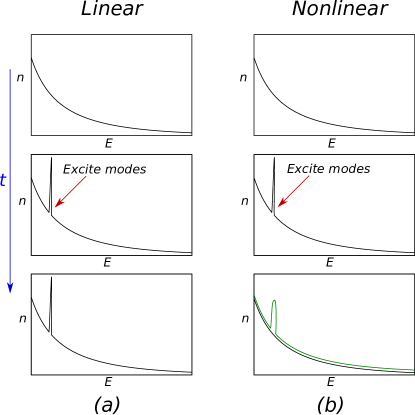
Figure 1: (a) A linear system of phonons. Top panel: The average occupation of a mode at energy $E$ versus $E$ in thermal equilibrium. Middle panel: Modes in a narrow band are excited. Lower panel: after long time, the distribution remains unaltered. (b) The same situation with nonlinearity present. Lower panel: The red curve, illustrates that the distribution at intermediate times as it relaxes back to the thermal result. The black curve shows the result after a long time, having relaxed back to the thermal result. (The curves have been slightly displaced for clarity).

But such non-thermal behavior is not expected to occur in most experimental situations. We would naturally expect, that in analogy with the classical case, that there will be an exchange of energy with other modes, causing an eventual relaxation of the system to thermal equilibrium, with a slightly higher temperature. How precisely this happens, even at the classical level, is not at all obvious, and so it makes sense to first briefly review how classical systems manage to thermalize. For a clear and more detailed exposition of the classical and a range of quantum approaches, the reader is invited to read Ref. Singh (2013).

I.3 Classical thermalization

To understand thermalization, we confine ourselves for the moment, to a range of important quantities that are at the heart of equilibrium statistical mechanics: equal time averages of observables. Consider some observable that varies as a function of time, $O(t)$, which could be, for example, the $z$ component of a dipole moment, or the momentum of a single atom in a crystal. We would like to find the time average of $O$, over an interval of time $\cal T$, that we will eventually extend to infinity. In most situations, calculating the value of momentum over all time is essentially impossible, and so it would seem that its time average would be as well.

However there is a way of understanding this situation that makes answering such questions quite manageable. We consider the phase space of a closed classical system, as illustrated in Fig. 2.

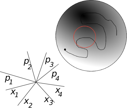
Figure 2: A two dimensional projection of phase space with 8 canonically conjugate variables $q_{1}\dots q_{4},p_{1}\dots p_{4}$. The black line corresponds to the path of the system over some time interval. The sphere corresponds to the points allowed by energy conservation. The red closed path corresponds to a periodic trajectory.

A complete description of the system is achieved by including all of the canonically conjugate coordinates. Say that there are $N$ positional degrees of freedom $q_{1}\dots q_{N}$ and $N$ momenta $p_{1}\dots p_{N}$. We can view those variables as a point in a $2N$ dimensional space, known as phase space, $\Gamma=\{q_{1}\dots q_{N},p_{1}\dots p_{N}\}$ . As time progresses, these coordinates will change as well, meaning that this point will move, as illustrated, tracing out a path. Because energy is conserved, we know that this path will reside on a surface of constant energy.

In general, this path will be very complicated. If it succeeds in getting arbitrarily close to every point on this surface, then the system is called “ergodic” Farquhar (1964); Jancel (2013). Ergodicity says, loosely speaking, that $\Gamma(t)$ will get arbitrarily close to every point on the constant energy surface given a long enough time. We also know from Liouville’s theorem, that the system will spend equal times in equal phase space volumes, so the trajectory will end up covering the ball uniformly. Such a path is shown in black in Fig. 2.

This means that instead of averaging an observable $O$ over time, $\langle O\rangle_{t}$, we could equally well average it over phase space with the constraint that we are confined to this constant energy surface. That’s a far easier problem to calculate mathematically. More precisely, regarding the observable as a function of phase space $O(\Gamma)$, we can then say Ma (1985)

$$\langle O\rangle_{t}=\frac{\int_{S}O(\Gamma)d\Gamma}{\int_{S}d\Gamma}$$ (1)

where we are integrating over a surface $S$ of constant energy. And this is precisely how averages are described in the classical “microcanonical ensemble”. It is also important to note that there other invariants, for example total system momentum, that might also be conserved. In these cases, the surface must also include these other invariants.

(a)                               (b)

Figure 3: (a) Example of Sinai billiards: Two hard core spheres move in free space with periodic boundary conditions. (b) Bunimovich Stadium. A point particle moves in free space confined to a stadium with hard walls. The stadium has semicircular sides and a straight mid-section.

In order for this to work, it would seem as if the system should be ergodic or at least close to it. There have been a few examples where it has been possible to prove ergodicity, most notably, a gas of an arbitrary number of hard spheres in some volume Sinai (1970); Simányi (2004, 2009); Szász (2008), often called “Sinai Billiards” as illustrated in Fig. 3(a). The proofs are quite involved, but the result tells us that time averages are calculable through the microcanonical ensemble formula. Another such system that has been proved to be ergodic Bunimovich (1979) is the “Bunimovich Stadium”, which describes the motion of a free particle inside a stadium with hard walls that are circular on the sides, and straight in the middle, see Fig. 3(b).

But there are also other systems, the are “integrable” where there are $N$ other invariants, meaning that these are constants of motion. Such a closed trajectory is schematically represented by the red curve in Fig. 2. Referencing our phonon example, the fact that the crystal does not thermalize is because of these extra invariants. In that case, each of these invariants is the energy of a single normal mode. A typical trajectory of such a system is therefore described by the combined motion of the normal modes, and will in general be quasi-periodic. However, integrable systems are unusual, and not expected generically. For example, any anharmonic term added, will make this problem non-integrable, or “generic”.

But in general, we do not expect that a generic classical system, for example a gas with Van-der Waals interactions, or a model of phonons with anharmonic terms, will be, strictly speaking, ergodic. For finite $N$, there has been a great deal of work on what happens in such systems. The Kolmogorov –- Arnold –- Moser (KAM) theorem tells us that for a weak anharmonic perturbation of order $\epsilon$, most phase space trajectories will continue to be quasi-periodic as in the integrable case. However as the strength of the anharmonicity is increased, the fraction of such quasiperiodic trajectories is expected to decrease. In real situations however we do not necessarily have very strong nonlinear terms in the Hamiltonian, so why does statistical mechanics work in these cases?

What is generally believed is that as $N\rightarrow\infty$, the range of $\epsilon$’s where a significant fraction of quasiperiodic orbits survives becomes vanishingly small Falcioni et al. (1991). Thus for an isolated system, for statistical mechanics to work, one needs to have large $N$. In most experimental situations this is usually not an problem, because $N$ is normally very large and therefore there will be a vanishingly small sets of initial condition where the trajectories are quasiperiodic, and therefore the system can be considered to be ergodic.

Related to ergodicity, is the idea of chaos. The idea is that two systems with slightly different initial conditions will evolve into systems that are have very different coordinates, $\Gamma_{1}(t)$ and $\Gamma_{2}(t)$. The rate of divergence can be characterized by their Lyapunov exponents. For example, for two Sinai billiards in some closed volume, the trajectories will be very sensitive to the initial conditions, and with every subsequent collision, $\Gamma_{1}(t)$ and $\Gamma_{2}(t)$ will diverge from each other more strongly. However ergodicity is not equivalent to chaos, a simple counter-example being a one dimensional harmonic oscillator, which is ergodic, but close trajectories do not diverge from each other. Thus ergodicity ensures that phase space is well stirred, but it does not ensure it is scrambled. However, for a large number of degrees of freedom, we expect that most systems will be ergodic and chaotic.

But in some contexts, thermalization does imply scrambling, and more formally this idea is called “mixing” Arnol’d and Avez (1968). This can be thought of qualitatively to be related to mixing paints but in a high dimensional space. There are many definitions for this, but it is says essentially understood as follows. Suppose we have an ensemble of systems with initial conditions in some arbitrarily small region, analogous to a drop of dye in water. Then after a sufficiently long time, the separate systems (analogous to dye molecules) will be spread uniformly over all of accessible phase space. Thus such a system loses all correlations with its state at an earlier time. Because of this, systems that are mixing will also be ergodic.

In practice, most large $N$ classical systems of physical relevance are strongly chaotic, so that they are very close to being strongly mixing and ergodic. Later on we will contrast such systems with well known quantum integrable systems.

I.4 Quantum chaos

Now we turn to trying to understand how chaos manifests itself in quantum mechanics. In fact, there is some debate over the term “Quantum Chaos” and Michael Berry prefers the term “Quantum Chaology” Berry (1987) because as we shortly discuss, quantum mechanics cannot manifest chaos to the same extent that was described above for classical mechanics. But there is definitely a set of phenomena that occur that are related to classical chaos in many strongly interacting quantum systems.

I.4.1 Random Matrices

One of the first studied and best examples of a strongly interacting quantum system that is quite isolated from its environment, is a heavy nucleus. Experimental data has been amassed for thousands of energy levels but they do not appear to follow any simple mathematical form, such as the Rydberg formula. Instead it appears that the levels are quite random Shriner et al. (1991) and can be well characterized statistically. In 1955, Wigner Wigner (1993) proposed using random matrices to understand the distribution of energy levels found experimentally, which turned out to be an extremely deep and insightful approach to adopt. His reasoning was quite general, and had nothing to do with the precise form of interactions in the nucleus, as QCD was unknown at the time. Since then, the same random matrix models have been shown to describe the statistics of a large number of interacting quantum systems.

The statistics of the eigenvalues of real symmetric random matrices map on to the classical statistical mechanics of one dimensional gas with repulsive logarithmic interactions, held together by an external quadratic potential. The position of a particle corresponds to an eigenvalue, so at finite temperature, the set of eigenvalues will look like a snapshot of this thermal system. This leads to a number of interesting properties, and the most clear signature is to look at a suitably normalized difference between adjacent levels. Because of the repulsive interactions, this leads to strong energy level repulsion. Wigner showed that the distribution of energy level differences is very close to

$$P(s)=\frac{\pi}{2}se^{-\pi s^{2}/4}$$ (2)

This fits the data on nuclei quite well Shriner et al. (1991). This also implies no energy degeneracies.

Because such problems are quite intensive numerically, the first direct calculation of quantum energy levels showing such a connection occurred in systems with a small number of degrees of freedom in the semiclassical regime, such as Sinai billiards Bohigas et al. (1984a). The remarkable similarity of the statistical properties of these energy levels to those of real symmetric random matrices led to the Bohigas-Giannoni-Schmit conjecture Bohigas et al. (1984b): That in fact, any classical system that is strongly chaotic, has corresponding quantum energy levels that have the same statistics as such random matrices (in the limit of high energy levels).

I.4.2 Chaos in classical versus quantum mechanics

We have seen that there is a well studied path to understanding thermalization in classical systems, and the key concepts there are chaos and ergodicity. We have also seen how classically chaotic systems appear to behave when quantized. But it is still not at all clear how thermalization can occur in quantum mechanics. Here are some differences between quantum and classical theories:

1. There are many extra invariants of motion in quantum mechanics. For example, any function of the Hamiltonian $f(H)$ because $[f(H),H]=0$. In particular any projector of an individual energy eigenstates $|E\rangle\langle E|$ will be a constant of motion. These constants of motion are there even with classically chaotic Hamiltonians. This is related to the next point.

2. Another way understanding this is to write the time dependent wave function as a spectral expansion

   $$|\psi(t)\rangle=\sum_{E}c_{E}e^{-iEt}|E\rangle,$$ (3)

   where $c_{E}=\langle\psi(0)|E\rangle$. $|\psi(t)\rangle$ has a constant of motion associated with every energy eigenvector. In this sense it appears analogous to integrals of motion in classical mechanics, that give rise to a similar (quasiperiodic) formula for phase space variables.

3. In order to discuss ergodicity, the central concept we used was that of phase space. But in quantum mechanics position and momentum do not commute. That is, it is not possible to simultaneously measure all momentum and positional degrees of freedom. Therefore the whole conceptual framework illustrated in Fig. 2 will not work. At a semiclassical level, one can think of wave packets of linear dimensions $\Delta x$, and momentum dispersion $\Delta p$ chosen such that $\Delta x\Delta p>\hbar$, but this wave packet will spread in time and this is only useful in the semiclassical limit.

Aside from these differences in the mathematical structure, at a physical level, classical and quantum thermalization appear very different, particularly for a system with a small number of degrees of freedom.

Consider two classical Sinai billiards in some volume, for example, a box with either hard wall or periodic boundary conditions. If we start off the system with arbitrary initial momenta and positions, despite its small size, we can still say that the system will “thermalize”. Eq. (1) will apply in this case and the only dependence that answer will have is on the systems total energy. Aside from that, there is no dependence on the initial conditions. For example, the momentum distribution will be isotropic. This will be the case for any choice of the radii of the two billiards. However if you make the radii zero, then no interaction between them is possible, and the system becomes integrable, in which case average values will depend on the initial conditions, because now the energy of the individual billiards is conserved. For example, now the momentum distribution will no longer be isotropic.

We can contrast with the quantized version of this problem. If we start off with two billiards of finite radii and start them off in an arbitrary initial state, we can calculate the time average of an observable. Using Eq. (3), we can calculate the time averaged expectation value of observable $\hat{O}$ Jancel (2013); Farquhar (1964); Penrose (1979),

$$\langle\langle\psi(t)|{\hat{O}}|\psi(t)\rangle\rangle_{t}=\sum_{E}|c_{E}|^{2}\langle E|{\hat{O}}|E\rangle$$ (4)

where here we assume no degeneracy, as is the case for the above example. This shows that observables depend on all of the coefficients $c_{E}$, and therefore depend sensitively on the initial condition.

Time averages for ergodic classical mechanical systems only depend on the total energy, whereas quantum mechanical systems depend on the details of the initial conditions. One might first believe that the reason for this difference is the linearity of quantum mechanics, and the nonlinearity of classical mechanics.

The perspicacious reader may notice that classical mechanics can be described as a linear equation quite analogous to the Schroedinger equation Koopman (1931); von Neumann (1932a); von Neumann (1932b), which evolves a probability amplitude, as opposed to Liouville’s equation, which evolves a probability. However for these kinds of equations, the eigenvalues are badly behaved Wilkie and Brumer (1997) which invalidates the derivation of Eq. (4) in this case.

At this point, we can see that thermalization cannot occur in general in a quantum system, as we have shown in the above example how it apparently fails to work for the case of two Sinai billiards. It went wrong because we have a small number of particles leading to a low density of states. As we shall now see, the situation greatly improves in the large $N$ limit.

II Statement of the problem

The central question of this discussion is to understand why and how an isolated system thermalizes.

For a large number of number of degrees of freedom, $N$, the density of states $n(E)$ is very large. This is proportional to $\exp(S(E)$, where $S(E)$ is the entropy. Because usually the entropy is extensive, $n(E)\propto(\exp(const\times N)$. This means that the average level spacing, which is inversely proportional to $n(E)$, is incredibly small. This plays an important role in understanding the nature of thermalization. Unlike classical mechanics, we can see from the discussion in the introduction of two billiards, that statistical mechanics is not expected to work for low lying energy states, and the results obtained will depend on details of the initial state. But we expect that statistical mechanics will emerge in the large $N$ limit.

To be more precise, we can start by posing a related but easier question. Suppose we have a pure state $|\psi(t)\rangle$ and an observable $\hat{O}$. As we discussed in the introduction, we can consider the time average of the observable $\langle\langle\psi(t)|{\hat{O}}|\psi(t)\rangle\rangle_{t}$ which according to (4) can be related to the expectation values of these operators in energy eigenstates, terms like $\langle E|{\hat{O}}|E\rangle$.

We want to know why this time average is in accord with the prescription of statistical mechanics. For an isolated system we can define the quantum mechanical version of the microcanonical ensemble discussed for classical systems in the introduction. Because energy levels are quantized, the microcanonical ensemble involves averaging over all eigenstates within an energy window $\Delta E$. For large $N$, this means that we can take $\Delta E$ to be very small, still much less than any energy scale in the problem, yet it contains an extremely large number of eigenstates. The microcanonical average at energy $E$ becomes:

$$\langle\hat{O}\rangle_{micro,E}=\frac{1}{\cal N}\sum_{E^{\prime}\in[E,E+\Delta E]}\langle E^{\prime}|{\hat{O}}|E^{\prime}\rangle.$$ (5)

Here $\cal N$ are the number of levels being summed over. What this formula is telling us, is that to obtain the correct time average of an observable, we calculate the expectation value of $\hat{O}$ for all energy eigenstates in an energy shell, and then average over all those results.

Why should this microcanonical average be the same as (4)? That is the central question that we want to discuss and is the hardest part of the justification of statistical mechanics. If that can be established, it is relatively straightforward to understand why the microcanonical average is equivalent to the canonical one

$$\langle\hat{O}\rangle_{canon}=\frac{1}{Z}\sum_{E}\exp(-\beta E)\langle E|{\hat{O}}|E\rangle.$$ (6)

where the normalization $Z$ is the partition function, and $\beta$ is the inverse temperature. The equivalence of ensembles can be understood by considering a subsystem $A$ much smaller than the rest of the system, $B$, and considering operators $\hat{O}$ that are local enough to only depend of degrees of freedom in $A$. Intuitively one can think of $B$ as acting as a heat bath of $A$ Reif (2009), but more rigorous derivations using steepest descent can be given Lax (1955). In fact the exponential function can be substituted for many other functions that decay quickly enough, and these can be shown to be equivalent to the microcanonical ensemble as well. The extremely fast rise in the density of states, multiplied by $\exp(-\beta E)$, yields a function that is very strongly peaked at one energy, which is the essential reason why the result looks microcanonical.

Now let us return to the microcanonical ensemble and discuss how thick an energy shell that we need to consider. It is useful to consider the temperature of a system at energy $E$, assuming that it does thermalize. Mathematically this means calculating the relationship between average energy and temperature $T$, using the partition function. The temperature sets a scale for the energy in Eq. (6) that tells us qualitatively as the available energy in single particle excitations. The average energy per particle $(E(T)-E(T=0))/N$, is another scale that that will be related to the temperature by a function that is independent of $N$ for local Hamiltonians. The change in the systems physical behavior when an additional energy $k_{B}T$ is added to it, is negligible. Thus choosing $\Delta E=k_{B}T$ in Eq. (5), means that the energy of the states that are contributing, are physically indistinguishable. Because of the large density of states, the average separation of levels is

$$\delta E\propto\exp(-S(E))\propto\exp(-const.N),$$ (7)

and is exceedingly small for macroscopic systems. Within an energy shell of thickness $k_{B}T$, there are an exponentially large number of states. Therefore, statistical fluctuations from eigenstate to eigenstate will be come negligible.

Viewed this way, we can rephrase our central question: why is (4) equivalent to (5)?

III Routes to understanding statistical mechanics

Everyone who has taken a course in statistical mechanics has heard some attempt to justify it. There are a number of different routes that have been taken and this section discusses the most popular ones.

III.1 Typicality

The idea of typicality is intimately related to empiricism. The Sun has risen for thousands of years, so we expect it will come up tomorrow. It may not, if say a planet sized object were to hit the Earth, but barring extremely unlikely events, we expect it to behave as it always has. Similarly, suppose we look at a “typical” quantum state of given total energy, and can show that it almost certainly will obey the laws of statistical mechanics. Then we expect that in any experiment that we perform on a particular state, it should with very high probability, obey statistical mechanics. This idea goes back to Schrödinger Schrödinger (1989) and has led to insights into many questions. Although its purported explanation for thermalization is criticized here, it is indeed very useful in understanding the ETH Tasaki (1998); Gemmer and Mahler (2003); Popescu et al. (2006); Goldstein et al. (2006); Linden et al. (2009); Müller et al. (2015).

In order to make this kind of argument more precise, a probability measure needs to be defined on the space of wave functions, that is, Hilbert spaces. It is easiest to assume that all wave functions with energy within a small range, $[E,E+\delta E]$ are weighted with equal probability. When a wavefunction is picked from this distribution, it defines a system in a pure state. One can ask how well expectation values of observables agree with the results from a microcanonical distribution.

A wavefunction can be written as in Eq. (3), at $t=0$. There are an extremely large number of coefficients $c_{E}$, and typically they will all be nonzero. The condition on the energy means that to be typical, the $c_{E}$ are drawn uniformly from the surface of a high dimensional hypersphere.

If we consider $\langle\psi|{\hat{O}}|\psi\rangle$ for any $|\psi\rangle$ with energy within this energy shell, then its value will depend on the choice of $|\psi\rangle$. We can ask what is $\langle\psi|{\hat{O}}|\psi\rangle$ when averaged over such $|\psi\rangle$. We can call this $\langle\hat{O}\rangle_{typical}$. And we can ask how much $\langle\psi|{\hat{O}}|\psi\rangle$ varies as we change $|\psi\rangle$.

Because we are averaging over a very large number $c_{E}$’s, it is not surprising that the fluctuations in $\langle\psi|{\hat{O}}|\psi\rangle$ are small. Also $\langle\hat{O}\rangle_{typical}$ is almost identical to $\langle\hat{O}\rangle_{micro}$, as in both cases, an average is being taken over a very large number of independent wavefunctions.

Thus if we pick a wavefunction drawn from this uniform distribution, we would expect $\langle\psi|{\hat{O}}|\psi\rangle$ to be extremely close to the microcanonical average. This has been shown to be rigorously the case in quite a few respects. For any small enough subsystem that is weakly coupled to the rest of the system, the expectation value of operators in it will agree with the canonical average, Eq. (6). In other words, typically small enough systems look completely thermal and the expectation value of any quantity will agree with results from the standard result from statistical mechanics Tasaki (1998); Gemmer and Mahler (2003); Popescu et al. (2006); Goldstein et al. (2006); Linden et al. (2009); Müller et al. (2015).

The main criticism of this approach is that in real experimental situations, the wave function is not typical. If your wave function was typical, then according to the above, you would be in thermal equilibrium. If that were the case, all macroscopic currents, such as those in neuronal action potentials, would be missing. You would not be able to process any information. Life is incompatible with thermal equilibrium and therefore we are decidedly not in a thermal state. We are in a state that is far from typical, composed of many macroscopic regions with different temperatures, chemical potentials, and pressures. The second law of thermodynamics also tells us that the Universe is not in equilibrium and therefore not in a typical state. Assuming that we are overwhelming likely to be in a typical state, we would predict a universe at constant temperature, and with an entropy that does not change in time. The fact that you are reading this now, proves that this assumption is incorrect.

But it has been possible to prove many useful theorems about typical states, and these have found many applications. So typicality remains an important approach to understanding statistical mechanics.

Another important general criticism of this approach will be given below for why this is not an adequate explanation of the central problem we wish to understand.

III.2 Ignorance of the system

“Statistical” often denotes the use of probabilistic reasoning, which normally connotes some uncertainty. This has been conflated to mean that statistical mechanics must have a probabilistic component due to a lack of information Jaynes (1957a, b); Tolman (1938). Some knowledge is uncertain because we cannot be bothered to find out more about it, for example the temperature right now in Tulsa Oklahoma. This is an example of knowledge that is subjective, because another reader could easily look up the answer. On the other hand, in quantum mechanics, most questions do not have an answer which is certain and this second class of objective uncertainty has been conflated with the first so for the moment, let us confine ourselves to classical statistical mechanics where there are no intrinsic uncertainties in a system’s evolution.

There has been a school of thought which has used a lack of knowledge to make physical predictions about systems at finite temperature. It is indeed true that it is extremely difficult to obtain the positions and momenta of gas in a room. But if someone did, this would not alter any physical outcomes (again at a classical level). Their knowledge wouldn’t change the room’s temperature, or pressure. Lack of knowledge at a classical level cannot be used to infer physical quantities. However if you follow this approach, you can use ignorance to “derive” the canonical or microcanonical distributions.

If one does not know any more than the energy of a system, then one can ask, what is the probability that it is in a particular microscopic configuration (or state). For example, when tossing a coin, without any information, you could say a priori, that there is equal probability that the outcome is a head or a tail. Similarly if you measured the $z$ component of spin, you could also assign it equal probabilities. Now suppose you were given 10 weakly interacting spins that were in a magnetic field. You can then ask what the probability distribution of configurations would be if you were given the total energy. Using ignorance, you can assign equal weights to all configurations that have the correct energy. This is mathematically equivalent to a microcanonical ensemble. Despite the fact that the prediction is based on a lack of knowledge, one can then perform experiments where you can measure precise spin configurations and see whether they do in fact agree with the microcanonical prediction. In many cases, of course, they do, giving some confirmation to this strangely illogical procedure.

This provides an explanation for the laws of statistical mechanics, at least when it works. The system needs to be in equilibrium and also not integrable, as we will discuss further below. But it is fundamentally flawed for the reasons above, and incapable of correctly predicting when the laws of statistical mechanics actually fail.

There are quite a few mathematical details left out in the brief summary given here, such as the maximization of the probability distribution, conditioned on energy or particle number constraints. And this involves some elegant mathematics. But this does not alter the fundamental flaw in this approach. Even at a classical level, the correct explanation for statistical mechanics involves ergodicity, which is something that does not come into this analysis in any way.

The situation is complicated by the addition of quantum mechanics, where the wave function represents a probability wave, and therefore the system is intrinsically probabilistic. However this only serves to make the argument more complicated. Fundamentally you can prepare a quantum state and know a lot about it. For example, in principle, it is possible to prepare a system so that all of the $c_{E}$’s in Eq. (3) are known. If this information is added, it will completely alter the resultant probability distribution according to this sort of reasoning, and will no longer look microcanonical, or canonical.

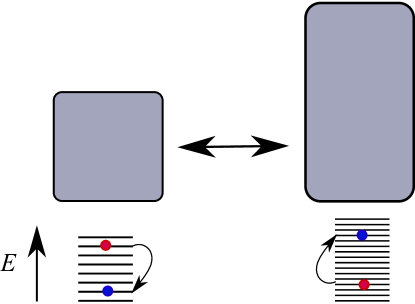
Figure 4: A small and system coupled weakly to each other. For short times, each system can be thought of as being isolated. Initially the energy levels of each of the systems is shown by the red dots. After a long time, they transition to new levels, shown as blue dots. After a long time, the smaller system explores a large number of separate states.

III.3 Open systems

With open systems, the system of interest is contact with a much larger one, considered to be a “heat bath”. The bath has properties that make it straightforward to obtain statistical mechanics for the system of interest. One justification for this is that it is impossible to have a truly isolated system, and therefore one must always consider a smaller system that is connected to a much larger one Blatt (1959); Gemmer et al. (2004). The smaller system exchanges energy with the larger system, and it is possible through a number of arguments, to derive the canonical distribution for the smaller system.

One intuitive explanation assumes a very weak coupling between the two systems as shown in Fig. 4. For times that are short enough, the two parts of the system will appear isolated, but for longer times, there will be an exchange of energy between them. Thus the energy in the smaller system will increase and decrease, sampling states of different energies. A time average over the smaller system will then yield a weighted average over different energy levels, depending on how much time is spent in the different states. It is straightforward to argue that this will be highly peaked function of energy, and thus equivalent to an ensemble average, for example Eq. (6). This kind of argument is often discussed in introductory textbooks, because of its relative simplicity Reif (2009). Not only does this approach sidestep the need for understanding the intricacies of a closed system’s dynamics, but can be very useful to derive approximate equations for the smaller system’s evolution, and these can be very valuable Lindblad (1976, 2001).

But what if the complete system has a quadratic Hamiltonian? This would not thermalize, so clearly there is a problem with the above approach. But we could allow the complete system to weakly couple to an even larger system, and hope that this would save this approach, unless the larger system was also quadratic, which would mean coupling yet again. These turtles all the way down arguments have an intuitive appeal but lack logical clarity.

III.4 Litmus test for these explanations

If we refer back to Fig. 1, and its discussion in the introduction, we see that not all system thermalize. If an explanation cannot distinguish between integrable and generic non-integrable dynamics, and predicts all such systems thermalize, it has to be incorrect. The above explanations all are incapable of making this distinction. At a classical level, explanations, such as using ignorance, cannot be correct as was already noted.

The fact that most systems do obey statistical mechanics, does not make these explanations correct, but it does not make these ideas without merit. Typicality is still a very useful mathematical result, that has applications to many areas even including numerical simulations. Reasoning using ignorance, or open systems, are relatively simple and intuitive. They provide a lot of intuition and guidance in understanding physics problems. When a system does thermalize, it is often very useful to divide it up into smaller and larger pieces, where open system arguments can be used to understand statistical fluctuations. Another interesting approach uses the large number of coefficients in Eq. (4) expected in experimentally realistic conditions to find a agreement with statistical mechanics Reimann (2008). Also it would be remiss not to mention an insightful approach provided by Von Neumann’s “Quantum Ergodic Theorem” von Neumann (2010), which was quite recently developed further Goldstein et al. (2010a, b). As shown recently, the assumptions that go into this theorem are essentially the same as assuming the ETH Rigol and Srednicki (2012).

A more predictive and fundamental understanding of thermalization, needs to be able to distinguish between the different physical behavior of generic systems, which are chaotic, and integrable systems. The analog of chaos in quantum mechanics has to be better understood in order to make progress understanding the origin of statistical mechanics.

The route taken here is to try to parallel the discussion of classical systems of the introduction. We want to understand if there is some analog of ergodicity and chaos that can be used to understand quantum statistical mechanics, that is Eq. (5). What special features of generic quantum systems allow thermalization, where as integrable systems do not?

IV Relation to Random Matrices

As was discussed in the introduction, there appears to be an intimate connection between strongly interacting quantum mechanical systems, and random matrices. The micro-structure of the energy levels appears identical for systems with high density of states. Other important physical properties also appear to be intimately tied to random matrices as well. In particular, how do we expect energy eigenstates of quantum mechanical systems to behave, and how is this related to random matrices?

IV.1 Semiclassical Limit

Studies of the semi-classical limit, of hard sphere systems, such as those shown in Fig. 3 have largely answered how energy eigenstates behave in the semiclassical limit. It’s simpler conceptually to think of a single particle in $3N$ dimensional space, with a momentum $\bf p$ and so that the Bunimovich stadium and Sinai Billiards just correspond to different boundary conditions of a stadium problem in higher dimension.

The energy eigenstates of non-interacting particles in free space are plane waves, in other words, can be chosen to be in a definite momentum state $|\bf p\rangle$. Classically, at a given energy, a total momentum momentum is $p^{2}/2m$. When go over to quantum mechanics, the general solution will be the sum (or integral) over plane waves on the energy shell, with amplitudes chosen to match the boundary conditions, in other words we are integrating over plane waves going at different angles. The analogy of classical ergodicity in this case, would be to have the amplitudes of the plane waves uniformly distributed in angles, rather than focused in particular directions. A number of theorems have been proved that show that this is the case in the semiclassical limit Shnirelman (1975, 1993); Zelditch et al. (1987); Colin de Verdière (1985); Helffer et al. (1987); Berry (1987, 1977). There is further numerical evidence supporting the idea that the amplitudes of these momentum states behave randomly Aurich et al. (1999).

The scope of the validity of the microcanonical average in the limit as $\hbar\rightarrow 0$, was further expanded by work that considered other Hamiltonians in the semiclassical limit and showed reasonable agreement with the microcanonical ensemble even for systems with a few degrees of freedom Feingold et al. (1985); Feingold and Peres (1986).

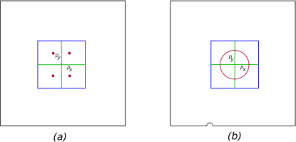
Figure 5: A comparison of a semiclassical integrable and non-integrable system comprising a particle moving in a stadium. The black stadiums in (a) and (b) represent the hard walls, and superposed in the middle are probability densities of energy eigenstates (red) shown in the momentum representation, characterized by the momentum $p_{x},p_{y}$. (a) Here the classical motion is integrable and only four momenta have nonzero probabilities. Classically corresponding to this, the particle will bounce off the walls alternating between these four discrete values of momenta. (b) The same situation where a small change to the boundary has been made, making the system non-integrable. Classically the momentum distribution will spread out isotropically over a circle. In the semi-classical case, the probabilities will also be spread out but their amplitudes will be uniformly distributed but random on this circle.

Therefore we have fairly good picture of a typical semiclassical energy eigenstate of hard sphere systems, that is eigenvalues of the Laplacian operator with appropriate boundary conditions. It will look like a random superposition of plane waves uniformly distributed over an energy shell. This is illustrated in Fig. 5 for the integrable case of a particle in a rectangular box in two dimensions, and rectangular box that has a small circular protrusion.

The randomness in the wavefunction is also mirrored by the randomness that appear in the distribution of eigenvalues which follow random matrix theory as well mentioned in the introductionBohigas et al. (1984b). The eigenvectors of a real symmetric random matrix will form a set of orthogonal random vectors, very similar to the orthogonal set of random vectors seen in the momentum representation of semiclassical billiards.

On the other hand, an integrable system will have completely different properties in the semiclassical limit, and random matrix models do not apply. Rather an extra set of invariants (such as the phonon example of the introduction) are used to construct energy eigenstates.

An important question to ask is whether or not the random matrix analogy only works in the semiclassical limit of small $\hbar$, or if it can be extended to systems where $\hbar$ cannot be taken as small. Underlying the analysis of energy level statistics and the randomness of wavefunctions was the need for a high density of energy levels. For small $N$, this would require a semiclassical approach, but for large $N$, systems at low temperatures and their associated energies, have correspondingly high density of states. We will ask in general how we can understand energy eigenstates for finite $\hbar$.

IV.2 Perturbing an integrable model

If a system is integrable, it will never thermalize. If now turn on an interaction to break integrability, we can ask what will happen. As discussed in the introduction in the context of KAM theory, for large $N$, it is generally believed that only a very small interaction is needed to destroy orbits with regular motion. And with Sinai Billiards, any non zero billiard radius will immediately destroy integrability. With the large $N$ classical situation in mind, in a quantum treatment, can we understand how a system will transition between integrable and non-integrable behavior? We will try to follow the same path as for the semiclassical limit of hard sphere systems Deutsch (1991).

Suppose we consider the Hamiltonian $H_{0}$ of the integrable system. We now add in a very weak integrability breaking term $H_{1}$ of order $\epsilon$,

$$H=H_{0}+H_{1}.$$ (8)

$H_{1}$ could be a two body interaction between particles in a gas, for example. As we have seen for hard core systems, semiclassically, in the basis of $H_{0}$, the eigenstates appear to be random superpositions. And the behavior of energy level spacings that we discussed, suggest that in this integrable basis, $\langle E^{0}_{i}|H_{1}|E^{0}_{j}\rangle\equiv h_{ij}$ can be can be taken to be a symmetric random matrix, but with the elements $h_{ij}$ being small.

Although there is some justification for this choice, it is still not clear how the elements $h_{ij}$ should be chosen. If we couple states of vastly different energies together, it will lead to catastrophic effects on the dynamics. The eigenvectors will now become completely delocalized in the energy basis of $H_{0}$, yielding nonsensical results.

Therefore from a physical perspective, $\langle E^{0}_{i}|H_{1}|E^{0}_{j}\rangle$ cannot have statistics that are independent of $i$ and $j$. In fact, if one calculates to second order in perturbation theory, the size of these elements, phase space arguments Deutsch (1991) show that $h_{ij}\sim\exp(-\beta|E_{j}-E_{i}|)$ for $\beta|E_{j}-E_{i}|\gg 1$. Here $\beta$ is the inverse temperature corresponding to a system with average energy $E_{i}$ (or $E_{j}$ because the difference between the two is so small in this context). With matrix elements decreasing away from the diagonal, we can take $h_{ij}$ to be a banded symmetric random matrix. Numerical confirmation of this bandedness had been given in the semiclassical limit quite early Feingold et al. (1989). A more recent study of Hubbard models Genway et al. (2012) showed a general banded structure for many quantities of interest. Bandedness is a crucial component of this matrix, as without it, the expectation values of operators would be completely unphysical, dominated by the highest energy states of the system. Further evidence for the banded nature will be given when discussion the ETH in the next section.

Thus the model in the integrable energy basis looks like a diagonal matrix, with increasing diagonal elements, $\langle E^{0}_{i}|H_{0}|E^{0}_{i}\rangle$, to which a banded symmetric random matrix is added Deutsch (1991). We need to understand some basic properties of eigenvectors of this kind of matrix. If the eigenvectors become still become delocalized this model would behave incorrectly. Fortunately, for such a model, or ones quite similar Wigner (1957), it can be shown that the eigenvectors are localized in energy.

This localization of eigenvectors in the integrable energy basis is an extension of what is found for billiard systems semiclassically. It says that a typical eigenstate of a non-integrable system is the random superposition of integrable states in some narrow energy shell

$$|E_{i}\rangle=\sum_{j}c_{ij}|E^{0}_{j}\rangle$$ (9)

and the $c$’s are the matrix of eigenvectors $\langle E_{i}|E^{0}_{j}\rangle$. Because $H_{1}$ is random the $c_{ij}$ will be also. Averaging over different random realizations of $H_{1}$, $\langle c_{ij}^{2}\rangle_{r}$ is strongly localized around $i=j$. This equation suggests that we can think about the energy eigenstates of the non-integrable system as the random superposition of the integrable eigenstates. Let’s compare this again to the sudden transition from integrable to non-integrable behavior you see with Sinai Billiards, going from a radius $r=0$ to $r>0$. For $r=0$, you have an ideal gas which will never thermalize. But $r>0$ but very small, eventually the system will thermalize due to particle collisions. In the quantum case, with nonzero $H_{1}$, you will get Eq. (9). How small does $H_{1}$ have to be? It turns out to be very small for large $N$. The relevant energy scale here is the energy level separation which decreases exponentially with $N$, so for an Avogadro’s number size system, this will involve numbers of size $\exp(-10^{23})$. We will discuss later, the transition for much smaller numbers of particles, as you would get in a numerical simulation or a cold atom experiment.

IV.3 Expectation values of nonintegrable eigenstates

The right hand side of Eq. (4) involves the expectation values of an operator $\hat{O}$ in energy eigenstates, $\langle E|{\hat{O}}|E\rangle$. Therefore this quantity is central to calculating time averages of operators, which in turn should be the same as microcanonical averages if statistical mechanics is to hold. Eq. (9) suggests that we can calculate such expectation values in terms of the energy eigenstates of integrable systems. Because the statistical mechanics of $H$ and $H_{0}$ should be the same to $O(\epsilon)$, we will see that expressing averages in terms of eigenstates of $H_{0}$ will be quite informative.

We can write

$$\langle E_{i}|{\hat{O}}|E_{i}\rangle=\sum_{kl}c_{ik}c_{il}\langle E^{0}_{k}|{\hat{O}}|E^{0}_{l}\rangle$$ (10)

But this involves the random eigenvectors $c$. These have mean zero and their statistics can be calculated reasonably well. One can ask what is the value of $\langle E_{i}|{\hat{O}}|E_{i}\rangle$ averaged over some small energy window of $E_{i}$, and what is the fluctuation in $\langle E_{i}|{\hat{O}}|E_{i}\rangle$. This is equivalent to averaging over the $H_{1}$ $\langle\dots\rangle_{r}$. Without going through the technical details, it is not much of a surprise to find that the cross terms in Eq. (10) vanish, yielding Deutsch (1991)

$$\langle E_{i}|{\hat{O}}|E_{i}\rangle=\sum_{k}\langle c^{2}_{ik}\rangle_{r}\langle E^{0}_{k}|{\hat{O}}|E^{0}_{k}\rangle$$ (11)

We can also consider the fluctuations in this expectation value

$$\sigma^{2}_{i}\equiv Var(\langle E_{i}|{\hat{O}}|E_{i}\rangle)$$ (12)

and show Deutsch (1991) it is extremely small proportional to $\exp(-S(E))\propto\exp(-const\times N)$. Because the $c_{ik}$’s are sharply peaked around $E_{i}=E_{k}$, Eq. (10) gives the microcanonical average of ${\hat{O}}$.

The intuitive picture of how non-integrable energy eigenfunctions appear from an integrable model, is not unlike what happens in the semiclassical case of hard walls, as illustrated in Fig. 5. An energy eigenstate is formed by the random superposition of states with very similar energies. Because of the amplitudes of all of these states are random, when forming expectation values of an operator, only its diagonal matrix elements contribute. This then gives expectation values of the operator averaged over an energy shell, which is precisely the microcanonical average.

It is also interesting that this arguments if we start an non-integrable point and perturb it which suggest that it may be of considerable generality.

IV.4 Off diagonal elements

It is also possible to calculate the properties of off-diagonal matrix elements $O_{ij}\equiv\langle E_{i}|{\hat{O}}|E_{j}\rangle$ in this model Reimann (2015). Their mean is zero and their variance can also be shown to be of magnitude to $\sigma^{2}_{i}\propto\exp(-S(E))\propto\exp(-const\times N)$. Their value will go to zero as $|E_{i}-E_{j}|$ become large. These off diagonal elements are important in determining the dynamical correlations, rather than expectation values of observables, averaged over time.

V The Eigenstate Thermalization Hypothesis

In the last section shows that for fairly general reasons, we expect that $\langle E|{\hat{O}}|E\rangle$ fluctuates very little as $E$ is varied and gives results in accord with the microcanonical distribution Deutsch (1991). This leads us to the “Eigenstate Thermalization Hypothesis” (ETH).

V.1 Statement of the Hypothesis I

The term “Eigenstate Thermalization” appears to have been first coined by Mark Srednicki Srednicki (1994) as a succinct description of how a single eigenstate can be thought of, as being in an equilibrium thermal state, in the sense now described.

Consider a finite isolated system, with a non-integrable Hamiltonian with $N$ degrees of freedom. The eigenstates $|E_{i}\rangle$ are solutions to ${\hat{H}}|E_{i}\rangle=E_{i}|E_{i}\rangle$. The solutions should also be separated by symmetry sector Santos and Rigol (2010). For example, as mentioned in the introduction, total momentum is often conserved, particularly in homogeneous systems with periodic boundary conditions. Only in a single sector can we assume that the $E_{i}$’s are non-degenerate.

Conjecture 1.

For a large class of operators, ${\hat{O}}$, we consider its expectation values $O_{ii}\equiv\langle E_{i}|{\hat{O}}|E_{i}\rangle$ as a function of $i$. We also consider the microcanonical average $\langle{\hat{O}}\rangle_{micro,E_{i}}$ as defined in Eq. (5). Then

$$O_{ii}=\langle{\hat{O}}\rangle_{micro,E_{i}}+\Delta_{i}$$ (13)

where $\Delta_{i}$ has zero mean and $\Delta_{i}^{2}$ has a magnitude of order $\langle{\hat{O}}^{2}\rangle_{micro,E_{i}}\exp(-S(E))\propto\langle{\hat{O}}^{2}\rangle_{micro,E_{i}}\exp(-const.\times N)$.

The sole fact that $O_{ii}$ varies very little among neighboring eigenstates implies that $\langle O_{ii}\rangle$ averaged over a small energy window must give the microcanonical average. Thus the ETH is really a statement about the small size of fluctuations of expectation values between eigenstates. It says that the microcanonical average for non-integrable systems, for most purposes, does not need to be taken at all, and a single eigenstate can be used.

The most unclear part of this statement is the class of operators to which it applies. There are clear examples of where this fails: For any function $f$, ${\hat{O}}=f({\hat{H}})$ commutes with ${\hat{H}}$ and therefore ${\hat{O}}_{ii}=f(E_{i})$. If $f$ is sufficiently poorly behaved, for example a $\delta$ function, then this will violate the hypothesis.

But such operators are global, involving all of the degrees of freedom in a system. The ETH is believed to work well for operators only involving a few degrees of freedom; for example, operators involving the momenta of three particles, and these do not have to be in the same region of space. But the exact limits of where it works and where it fails are still not clear. It is generally believed to be valid in most non-integrable systems when ${\hat{O}}$ involves operators in some local region. In fact it has been argued that for entanglement entropy in the case of two weakly coupled systems similar to the random matrix models considered above, that the smaller system can be almost as large as half the system Deutsch (2010). And this bound has been argued to hold for more general quantities for non-integrable systems as well Garrison and Grover (2015).

The exceptions to the ETH are for systems obeying Many Body Localization Altshuler et al. (1997); Basko et al. (2006); Imbrie (2016); Huse et al. (2013); Nandkishore and Huse (2015). These are very unusual systems that violate the ETH even though the system is non-integrable. We will discuss the validity of the ETH further in subsequent sections.

The way that the ETH has been defined above, is still a bit sloppy in another way. When we gave the size of the $\Delta_{i}$’s, it is exponentially small in $N$. However Hilbert space is exponentially large and we have not defined the distribution of $\Delta$’s. It still might be possible that an exponentially small fraction of eigenstate do not obey the ETH and have expectation values significantly different from the microcanonical ensemble. This can be thought of as the weak ETHBiroli et al. (2010a).

On the other hand, if we are to say that $O_{ii}$ is always very close microcanonical, for all $i$, this means we have the strong ETH. One might think that the distinction between the weak and strong ETH is not important. However even for integrable systems, typical states as noted above, give thermal averages. In fact, all but a vanishingly small number of eigenstates, will be in this category and can exhibit the weak ETH Müller et al. (2015). There have been some interesting non-integrable models that have been devised, that show an exponentially small number of microcanonical violating eigenstates Mori (2016); Mori and Shiraishi (2017), but their interpretation is still the subject of some debate Mondaini et al. (2017); Shiraishi and Mori (2017).

V.2 Statement of the Hypothesis II

The statement of the ETH has been further expanded to include the behavior of off-diagonal matrix elements. This is not necessary to understand how time averages are equivalent to ensemble averages. However, among other things, it is important in the understanding of dynamic correlation functions, and the approach to equilibrium Srednicki (1994, 1999); Khatami et al. (2013); D’Alessio et al. (2016). Here we more generally consider $O_{ij}\equiv\langle E_{i}|{\hat{O}}|E_{j}\rangle$. For $i\neq j$ the hypothesis is that, $O_{ij}=\Delta_{ij}$ where $\Delta_{ij}$ appears stochastic and has similar statistics to those described for Eq. (13), but now there are two relevant energies $E_{i}$ and $E_{j}$. These elements are therefore extremely small. Because the statistics of this quantity should vary smoothly as a function of $E_{i}$ and $E_{j}$, we can try to quantify this for a single system by performing averages over the nearby energy levels of $i$ and $j$, $\langle\dots\rangle_{n}$, so that we can write

Conjecture 2.

$$\langle|O_{ij}|^{2}\rangle_{n}=\langle{\Delta_{i}}^{2}\rangle_{n}F(E_{i},E_{j})$$ (14)

with $\Delta_{i}$ is the fluctuation in the $O_{ii}$’s described in Eq. (13). $F$ is a function of order unity for $E_{i}=E_{j}$ that goes to zero as $|E_{i}-E_{j}|$ becomes large.

Defining $\overline{E}_{ij}\equiv(E_{i}+E_{j})/2$, this can be written somewhat more symmetrically as

$$\langle|O_{ij}|^{2}\rangle_{n}=\langle{\hat{O}}^{2}\rangle_{micro,\langle E\rangle_{ij}}f(\overline{E}_{ij},E_{i}-E_{j})\exp(-S(\overline{E})/2)$$ (15)

where now $f(\overline{E}_{ij},E_{i}-E_{j})=F(E_{i},E_{j})$, describes a function that goes to zero when $|E_{i}-E_{j}|$ becomes large.

The $O_{ij}$ cannot in general be zero however. For example if we consider an operator $\hat{A}$ being the square root of $\hat{O}$, that is ${\hat{O}}={\hat{A}}^{2}$, then

$$\langle E_{i}|({\hat{A}}-A_{ii})^{2}|E_{i}\rangle=\sum_{j\neq i}|A_{ij}|^{2}$$ (16)

The left hand side is not small and is non-negative. The right hand side are terms that appear in the off-diagonal matrix elements that appear in this hypothesis. What this implies is that the off-diagonal matrix elements must be quite evenly distributed or this hypothesis would be violated.

V.3 Thermalization

Now we return to the situation illustrated by Fig. 1. An isolated system is put in a nonequilibrium state, and we ask if it will eventually return to equilibrium or stay in a nonequilibrium state. To identify if the system is in equilibrium, we ask if time averages of observations are in agreement with equilibrium statistical mechanics. This requires that $\langle\langle\psi(t)|{\hat{O}}|\psi(t)\rangle\rangle_{t}$ gives the average predicted from statistical mechanics.

It is worth noting that the averages predicted by quantum statistical mechanical ensembles are incorrect in situations where the system is in a macroscopic superposition, as exemplified by Schroedinger’s cat. We should expect that a precise treatment of time averages will yield a result that can include this possible initial state.

Eq. (4) tells us how time averages can be related to expectation values of eigenstates. If we assume the ETH, then this becomes to within small corrections

$$\langle\langle\psi(t)|{\hat{O}}|\psi(t)\rangle\rangle_{t}=\sum_{E}|c_{E}|^{2}\langle{\hat{O}}\rangle_{micro,E_{i}}$$ (17)

If the coefficients $c_{E}$ are strongly clustered around one energy, then because $\langle{\hat{O}}\rangle_{micro,E_{i}}$ is smoothly varying, this will also yield the microcanonical, or equivalently, the canonical average. On the other hand, it the $c$’s are not clustered around one energy, as is the case for a macroscopic superposition, then this time average will yield microcanonical values of observables weighted over the probability that they are in one of those superpositions. This is precisely what one would expect should happen in such cases.

Therefore for long enough times, the system will eventually return to a state of thermal equilibrium, at least when probed with observables for which the ETH is satisfied. This argument does not tell us how long one has to wait. The times necessary for Eq. (4) to be satisfied can be extremely long. But at the same time we also know that relaxation for some systems are extremely long even for an open system in contact with a heat bath. All we can say from the ETH is that equilibrium will eventually be achieved.

The crucial qualitative idea behind the ETH, is that each eigenstate is itself “thermal”, giving the same results as for averages in open systems in contact with a heat bath. One way to think about this is that a small number of degrees of freedom of the isolated system can be considered a subsystem and the rest of the system can act as a heat bath which is expected to yield thermal properties for the degrees of freedom being observed.

V.4 Does thermalization imply the ETH?

It is worth considering if there may be some alternatives to the ETH which can also explain the experimental observation that all real systems thermalize. It is also not clear whether or not the ETH is really a useful way of understanding thermalization because, as stated above, even integrable models satisfy the weak ETH.

From a theoretical perspective, both of these questions have been addressed. Suppose that we have an isolated system and view it as being divided into two, a system of interest, $A$ and the rest, $B$, which can be thought of as a bath for $A$. We now consider starting the system out of equilibrium, in an arbitrary product state of $A$ and $B$. If all such initial states result in the thermalization of $A$, this requires that the ETH hold. But it requires that the ETH hold in the strong sense, that all energy eigenstates are thermal. If this was not the case, there would be certain initial product states that would not thermalize.

Therefore what we have learned is that most systems have eigenstates that give microcanonical answers, whether or not they thermalize properly or not. In order to get thermalization, we need all eigenstates to give microcanonical averages.

This situation is not completely settled however, because it is not clear that all initial product states are experimentally realizable. And there are certainly examples of systems that do not obey this strong version of the ETH, but rather the weak version, but will still be able to thermalize some large class of initial states, but certainly not all of them Mori and Shiraishi (2017). It would indeed be very interesting if there existed some experimental isolated systems that could be shown to fail to thermalize from certain states that were carefully prepared. This would imply that statistical mechanics was not generally valid, opening up many interesting possibilities. Barring this possibility, this is quite compelling evidence that the ubiquity of thermalization seen experimentally, implies the strong version of the ETH.

V.5 Entropy and the ETH

Another important quantity that is still not well understood is the entropy of a system and indeed has many definitions. The Von Neumann entropy for a system with density matrix ${\hat{\rho}}$ is $S_{VN}({\hat{\rho}})=-\mathrm{tr}{\hat{\rho}}\ln{\hat{\rho}}$. For an isolated system in a pure state this is zero. The von Neumann entropy represents a lack of knowledge about a system, but not what is measured in thermodynamic experiments. But is there a way of defining thermodynamic entropy in an isolated system?

The entanglement entropy is often used as a measure of mutual information between two systems. Suppose we take an isolated system in a pure state, and divide into two subsystems $A$ and $B$. Then the reduced density matrix for $A$, ${\hat{\rho}}_{A}=\mathrm{tr}_{B}{\hat{\rho}}$, will in general become mixed because it is entangled with $B$. The entanglement entropy between $A$ and $B$ is defined to be $S_{AB}\equiv S_{VN}({\hat{\rho}}_{A})$.

We cannot directly apply the ETH to this problem because the entanglement entropy cannot be written as the expectation value of an observable. But the mathematics of this problem are quite closely related to the ETH. Theoretical argumentsDeutsch (2010) and numerical workDeutsch et al. (2013); Santos et al. (2011) indicate that this is indeed related to the thermodynamic entropy. For homogeneous systems in the limit of large $N$, finite energy eigenstates give an entanglement entropy that is equal to the thermodynamic entropy of the smaller of $A$ and $B$. This gives an explicit prescription for how to relate thermodynamic entropy to the microscopic description of the system in terms of its wavefunction. For integrable systems, this connection no longer holds for energy eigenstates, which shows the underlying importance of quantum chaos in the validity of thermodynamics.

This way of describing entropy, via entanglement, has no clear classical analog. Classically, entropy can be thought of as the amount of phase space explored by the system. To understand how this can increase in time, degrees of freedom are often coarse grained. It has been recently been shown Šafránek et al. (2017, 2017) that this idea of coarse graining can be extended to quantum mechanics by making sequential observations of different observables. For example, one can observe coarse grained positional degrees of freedom and then energy. This allows one to calculate the probabilities of each of these coarse grained bins, and construct a Gibbs entropy. For non-integrable systems by using the same random matrix model employed in understanding the ETH Deutsch (1991), this can also be shown to lead also to the thermodynamic entropy when the system is in an energy eigenstate.

With either definition of entropy, one ends up with the same thermodynamic entropy as one would have starting in a thermal state. But it is necessary for the system to be non-integrable in order for these results to hold.

VI Numerics

Pioneering initial numerical work on quantum systems with a large number of degrees of freedom Jensen and Shankar (1985) was hampered by the limited computational power available at the time. This led to a slightly unclear picture of eigenstate thermalization. At these system sizes, there was not a large distinction present between integrable and non-integrable systems, but the agreement with statistical mechanics was seen to depend on the choice of the observable and “good” ones appeared to be necessary in order to obtain this agreement. With larger system sizes that are easily achievable on todays computers, the distinction between integrable and non-integrable systems is much more apparent, and it is also clear that the agreement with statistical mechanics holds over a much wider class of observables, in agreement with the above theoretical arguments.

The main tool for studying the ETH numerically is exact diagonalization. This is a technique that is used to diagonalize the Hamiltonian of a discrete system. For example, Hubbard models, that allow hopping of particles between different sites with some local interaction between particles. Another commonly used type of system are ones involving spin degrees of freedom on a lattice. Because of the exponential growth of Hilbert space with the number of particles, and lattice sites, only relatively small systems are accessible this way, in the neighborhood of 25 lattice sites. There have been a wide range of studies of this type that have given us enormous insight into the nature of thermalization. The ETH has been observed in a wide variety of these lattice systems Rigol et al. (2008); Santos and Rigol (2010); Rigol (2009a, b); Rigol and Santos (2010); Khatami et al. (2013); Sorg et al. (2014); Biroli et al. (2010b); Neuenhahn and Marquardt (2012); Steinigeweg et al. (2013); Beugeling et al. (2014a); Kim et al. (2014); Steinigeweg et al. (2014); Khodja et al. (2015); Beugeling et al. (2015); Fratus and Srednicki (2015); Geraedts et al. (2016).

Today, even on a modest laptop, useful information can quite easily be obtained. As an example, consider for hard core bosons(HCB) in one dimension, with nearest neighbor (NN) and next nearest neighbor (NNN) interactions that cannot occupy the same site Santos and Rigol (2010). They evolve according to the Hamiltonian

$$\begin{split}H_{B}=\sum_{i=1}^{L}&\left[-t\left(b_{i}^{\dagger}b_{i+1}+h.c.\right)+Vn_{i}n_{i+1}\right.\\ &-\left.t^{\prime}\left(b_{i}^{\dagger}b_{i+2}+h.c.\right)+V^{\prime}n_{i}n_{i+2}\right].\end{split}$$ (18)

Here we are summing over all lattice sites $L$. $b_{i}$ and $b_{i}^{\dagger}$ are the boson annihilation and creation operators, respectively, for site $i$. $n_{i}=b_{i}^{\dagger}b_{i}$ is the boson local density operator. The NN and NNN hopping strengths are respectively $t$ and $t^{\prime}$. The interaction strengths are $V$ and $V^{\prime}$ respectively. Here we take $\hbar=t=V=1$.

This model is considered with periodic boundary conditions, meaning that there is translational invariance and particle number conservation. Therefore $H_{B}$ divides into independent blocks corresponding to different total momenta $k$. In this example we take $k=1$.

We can compare a non-integrable with an integrable choice of parameters to see how expectation values depend on energy. The choice $V^{\prime}=t^{\prime}=0.96$ corresponds to a non-integrable set of parameters, while $V^{\prime}=t^{\prime}=0$ is integrable. Here, somewhat arbitrarily, we consider the expectation value of $n_{1}n_{2}$, in different energy eigenstates, with $L=17$ lattice sites and the number of particles of $6$. Fig. 6 plots these expectation values for these two cases.

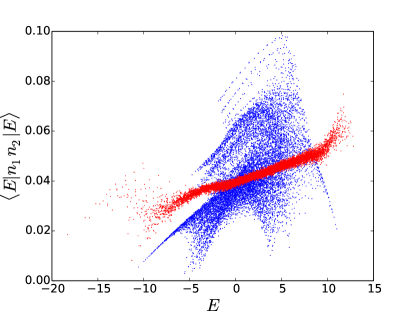
Figure 6: Numerical results for the hard core boson model of Eq. (18) for 6 particles on 17 lattice sites. The expectation value for the observable $n_{1}n_{2}$, corresponding to the probability that two particles will be next to each other, plotted for different energy eigenstates. The blue points represent the integrable case $V^{\prime}=t^{\prime}=0$, whereas the red points correspond to the non-integrable case $V^{\prime}=t^{\prime}=0.96$

In general, as the size of a non-integrable system increases, the fluctuation in expectation values decreases. Unfortunately, due to the exponential growth of Hilbert space, one does not expect to be able to simulate systems of even $100$ particles in the future, except perhaps with quantum computers. However much has been learnt about such isolated quantum systems by performing such numerical experiments, partly because one expects a rather rapid decrease in fluctuation as predicted by the Eq. (13), and verified numerically Beugeling et al. (2014b).

Many interesting things have been learned from studies of this kind, and allow us to answer questions that are very difficult to study by purely analytic means.

For finite size simulations, one can tune how far one is away from integrability. For example, in the hard core boson model above, those parameters are $t^{\prime}$ and $V^{\prime}$. For the small systems that are accessible by exact diagonalization, the ETH breaks down for finite $t^{\prime}$ and $V^{\prime}$, leading to a lack of thermalization Rigol (2009a). An interesting question to ask is how this range of non-thermal parameters varies with system size is increases. Does the range where the ETH holds increase to all non-zero $t^{\prime}$ and $V^{\prime}$ as one approaches the thermodynamic limit? Initial numerical evidence on gapped systems supported that the ETH works better for larger system sizes Rigol and Santos (2010). Based on analysis of scaling of the participation ratio of eigenstates in an operator’s eigenbasis, it was argued that indeed the ETH should be valid for any non-integrable parameters in the thermodynamic limit Neuenhahn and Marquardt (2012).

Another interesting question is whether or not numerical evidence shows that the ETH is valid in the strong sense as described in Sec. V.1. Numerical evidence on lattice systems appears to support that it actually does Kim et al. (2014). By explicitly searching for eigenstates where expectation values are “outliers”: far away from their mean value, one can analyze how these scale with system size. The behavior of the most extreme outliers as a function of system size, gives strong numerical evidence that even these obey the ETH.

Is the random matrix motivation for the ETH of Sec. IV nothing more than a happy coincidence, or is this the actual scenario for which it comes about? Aside from much earlier numerical work analyzing the statistics of energy eigenstates and eigenvalues Feingold and Peres (1986), one can look at the ratio fluctuation sizes of off diagonal matrix elements compared to diagonal elements. When compared with the results of random matrix theory, the results agree very well for large enough systems Mondaini and Rigol (2017).

There is further evidence Geraedts et al. (2016) that the connection of interacting systems to random matrix theory is the underlying reason for the validity of the ETH. This comes about by studying periodically driven Floquet systems D’Alessio and Polkovnikov (2013); Lazarides et al. (2014); Ponte et al. (2015). Ref. Geraedts et al. (2016) studied systems that could either be in a many body localized, or in a thermal phase. They studied the entanglement spectrum of such systems. In this case, they did so by tracing over half of their system and then considered the logarithm of their resultant reduced density matrix. Regarding this as a kind of entanglement Hamiltonian, its spectrum could be studied numerically. In the case of no driving, although they considered half of the system, they still found good agreement with the ETH in the thermal phase, supporting a strong version of it Garrison and Grover (2015). On the other hand, for periodic driving in the thermal phase, such systems heat up to infinite temperature Ponte et al. (2015), where ETH would then predict a trivial entanglement Hamiltonian equal to zero. Of course we expect corrections to this, and these can be studied numerically. What is quite interesting about these corrections, is that they also agree quite well with random matrix theory.

VII Relation to experiment

Sec. III gave routes to understanding the origin of statistical mechanics. It is not clear why any one but a dyed-in-the-wool theorist would care why it works, as it seems so clear that it does. But as we have seen, isolated integrable systems are not expected to produce systems that properly thermalize. Then again, quantum isolated integrable systems would seem very hard to produce experimentally.

The situation has changed dramatically over the last decade or so. There are now many experimental groups investigating the properties of atoms trapped and isolated from the outside world at very low temperatures, down to picoKelvin. These gases are typically quite dilute with a number of density of order $10^{14}/cm^{3}$. They are confined through magnetic or optical means and the confinement can be of many forms, such as a harmonic potential, or optical lattice Levin et al. (2012); Langen et al. (2015). These isolated systems can have coherence times of seconds, while typical relaxation times are often in the millisecond range Hofferberth et al. (2007), meaning that questions about isolated systems, that were purely theoretical twenty years ago, can now be tested experimentally. Furthermore control parameters, such as magnetic field can be used to tune the two-body interaction via the Feschbach resonance Chin et al. (2010).

In particular, the difference between integrable and non-integrable systems is very clear when starting the system out of equilibrium, similar to the scenario considered in the introduction. A number of one dimensional experimental systems are equivalent to integrable models Kinoshita et al. (2006), and very long lived momentum oscillations are observed. In contrast to such integrable models, which have very long lived non-equilibrium behavior, higher dimensional situations thermalize very rapidly Kinoshita et al. (2006). But although many aspects of these experiments are well described by theory, it is difficult to produce energy eigenstates in order to directly test the ETH. These experiments do show that isolated non-integrable quantum systems placed out of equilibrium, do approach the results predicted from statistical mechanics, on a time scale far smaller than their decoherence time.

A general lesson that has been learnt from these kinds of experiments is that many of the traditional approaches to understanding quantum statistical mechanics not only fail the theoretical litmus test described in Sec. III.4, but also fail to predict real experiments: There really is different behavior seen based on integrability, and not all isolated systems do thermalize over experimentally important timescales.

In fact not only is thermalization not seen experimentally in integrable models, but also in some random disordered systems that are believed to exhibit “Many Body Localization” Choi et al. (2016), mentioned in Sec. V. Not only can observables such as density and momentum distribution be measured, but quantities related to entropy. In an optical lattice experiment Kaufman et al. (2016), with 6 rubidium atoms, the second order Rényi entropy was determined by an ingenious method of interfering two copies of the system. The growth of entanglement could be assessed throught this Rényi entropy, and this entropy grew and saturated as predicted from ensemble statistical mechanical calculations. Thus despite the small system size, thermalization was evident.

These experiments have also allowed the probing of systems that are much larger than those that can be analyzed numerically, yet they still are quite precise, are highly tunable, and allow the measurement of many local observables. In this way, they act as an intermediary between solid state experiments that lack this precision, and numerics, which cannot attain such system sizes.

VIII Conclusions

The Eigenstate Thermalization Hypothesis is considered by most researchers now to be the major conceptual tool in understanding how quantum mechanics leads to thermalization. Among other things, it allows is to understand how the time averages of measurements give rise to the laws of statistical mechanics. In order to make headway, it makes sense to look at an isolated system where outside sources cannot influence the dynamics. The most basic statistical mechanical concept in that case, is the microcanonical ensemble. The microcanonical ensemble considers energy states withing a shell of width $\Delta E$, of which there are normally very many in the thermodynamic limit, even with very small $\Delta E$. The assumption of statistical mechanics is that time averages of observables are given by expectation values averaged over all states within $\Delta E$. The ETH says that $\Delta E$ can be taken to be so narrow as to include just a single energy.

An intuitive way of understanding the ETH, is to think of dividing the system into a smaller and larger region. Even for an energy eigenstate, you can then think of the larger region as acting as a thermal “bath” for the smaller region. The ETH says that for the system in any energy eigenstate, measurements on only the smaller the region are equivalent to a system at the appropriate equivalent temperature. As discussed in this review, this will not work for an integrable system, for reasons that are similar to the explanation in classical mechanics. In this sense, the ETH serves a similar purpose as ergodicity, in connecting the microscopic dynamics to statistical mechanics.

The underlying explanation for the ETH appears to have to do with the relationship between non-integrable quantum systems and random matrix theory. At a detailed microscopic level, at unimaginably small energy scales, the energy level spacing statistics fit very well with random matrix models. And even the energy eigenstates show a strong connection with random matrices. The ETH is a consequence of this random matrix description, a statement that is supported by detailed numerics for large enough systems Mondaini and Rigol (2017).

Aside for the current focus of the ETH in condensed matter and cold atom systems, the ETH is now been used increasingly in the study of quantum gravity, wormholes and firewalls. For example the “ER=EPR” conjecture of Maldacena and Susskind Maldacena and Susskind (2013) considers how two black holes connected by a wormhole are related to the entanglement between them. This has been analyzed using the ETH Marolf and Polchinski (2013). In another work, it has been proposed that the ETH can be applied to the metric in quantum gravity Khlebnikov and Kruczenski (2014). As it turns out, understanding the microscopic structure of eigenstates is important in a lot of applications.

It might seem odd that a statement about energy eigenstates for macroscopic systems would be so helpful conceptually in understanding thermalization. The time it would take to prepare a system in such an eigenstate is proportional to $\exp(S(E))$, which makes it completely inaccessible in most experimental circumstances. But to check for ergodicity in a classical system also requires unattainable measurement times, yet it is still crucial in understanding thermalization in that case. In both the quantum and classical cases, these sorts of concepts allow one to distinguish behavior that can be measured experimentally, such as the ability to thermalize. And in the quantum case the structure is perhaps even richer, allowing for the existence of exotic systems that exhibit Many Body Localization Nandkishore and Huse (2015), as briefly mentioned earlier. These will likely continue to yield interesting new phenomena. And there are likely to be other still undiscovered kinds of thermalization behavior that exist. For example, the idea of “Quantum Disentangled Liquids” has been proposed, where a system consisting of two different kinds of particles is only partially thermalized Grover and Fisher (2014). There are many reasons to believe that the recent focus in this area will continue to lead to many new surprises.

IX Acknowledgements

The author wishes to thank Richard Montgomery and Sergei Tabachnikov for an illuminating exchange on rigorous results for classical Sinai Billiards. This research was supported by the Foundational Questions Institute fqxi.org.

References

- Schrödinger (1927) E. Schrödinger, Annalen der Physik 388, 956 (1927).
- von Neumann (2010) J. von Neumann, The European Physical Journal H 35, 201 (2010).
- Deutsch (1991) J. M. Deutsch, Phys. Rev. A 43, 2046 (1991).
- Srednicki (1994) M. Srednicki, Phys. Rev. E 50, 888 (1994).
- Rigol et al. (2008) M. Rigol, V. Dunjko, and M. Olshanii, Nature 452, 854 (2008).
- D’Alessio et al. (2016) L. D’Alessio, Y. Kafri, A. Polkovnikov, and M. Rigol, Advances in Physics 65, 239 (2016).
- Srednicki (1996) M. Srednicki, Journal of Physics A: Mathematical and General 29, L75 (1996).
- Srednicki (1999) M. Srednicki, Journal of Physics A: Mathematical and General 32, 1163 (1999).
- Khatami et al. (2013) E. Khatami, G. Pupillo, M. Srednicki, and M. Rigol, Phys. Rev. Lett. 111, 050403 (2013).
- Altshuler et al. (1997) B. L. Altshuler, Y. Gefen, A. Kamenev, and L. S. Levitov, Phys. Rev. Lett. 78, 2803 (1997).
- Basko et al. (2006) D. Basko, I. Aleiner, and B. Altshuler, Annals of Physics 321, 1126 (2006).
- Imbrie (2016) J. Z. Imbrie, Journal of Statistical Physics 163, 998 (2016).
- Huse et al. (2013) D. A. Huse, R. Nandkishore, V. Oganesyan, A. Pal, and S. L. Sondhi, Phys. Rev. B 88, 014206 (2013).
- Nandkishore and Huse (2015) R. Nandkishore and D. A. Huse, Annu. Rev. Condens. Matter Phys. 6, 15 (2015).
- Marolf and Polchinski (2013) D. Marolf and J. Polchinski, Physical Review Letters 111, 171301 (2013).
- Levin et al. (2012) K. Levin, A. Fetter, and D. Stamper-Kurn, Ultracold Bosonic and Fermionic Gases, Vol. 5 (Elsevier, 2012).
- Langen et al. (2015) T. Langen, R. Geiger, and J. Schmiedmayer, Annual Review of Condensed Matter Physics 6, 201 (2015).
- Singh (2013) N. Singh, Modern Physics Letters B 27, 1330003 (2013).
- Farquhar (1964) I. E. Farquhar, Ergodic theory in statistical mechanics (Interscience, 1964).
- Jancel (2013) R. Jancel, Foundations of Classical and Quantum Statistical Mechanics: International Series of Monographs in Natural Philosophy, Vol. 19 (Elsevier, 2013).
- Ma (1985) S. K. Ma, Statistical Mechanics (World Scientific, 1985).
- Sinai (1970) Y. G. Sinai, Uspekhi Matematicheskikh Nauk 25, 141 (1970).
- Simányi (2004) N. Simányi, in Annales Henri Poincaré, Vol. 5 (Springer, 2004) pp. 203–233.
- Simányi (2009) N. Simányi, Inventiones mathematicae 177, 381 (2009).
- Szász (2008) D. Szász, Discrete & Continuous Dynamical Systems-A 22, 427 (2008).
- Bunimovich (1979) L. A. Bunimovich, Comm. Math. Phys. 65, 295 (1979).
- Falcioni et al. (1991) M. Falcioni, U. M. B. Marconi, and A. Vulpiani, Physical Review A 44, 2263 (1991).
- Arnol’d and Avez (1968) V. I. Arnol’d and A. Avez, Ergodic problems of classical mechanics (WA Benjamin, 1968).
- Berry (1987) M. V. Berry, in Proceedings of the Royal Society of London A: Mathematical, Physical and Engineering Sciences, Vol. 413 (The Royal Society, 1987) pp. 183–198.
- Shriner et al. (1991) J. Shriner, G. Mitchell, and T. Von Egidy, Zeitschrift für Physik A Hadrons and Nuclei 338, 309 (1991).
- Wigner (1993) E. P. Wigner, in The Collected Works of Eugene Paul Wigner (Springer, 1993) pp. 524–540.
- Bohigas et al. (1984a) O. Bohigas, M. J. Giannoni, and C. Schmit, Phys. Rev. Lett. 52, 1 (1984a).
- Bohigas et al. (1984b) O. Bohigas, M. Giannoni, and C. Schmit, Journal de Physique Lettres 45, 1015 (1984b).
- Penrose (1979) O. Penrose, Reports on Progress in Physics 42, 1937 (1979).
- Koopman (1931) B. O. Koopman, Proceedings of the National Academy of Science 17, 315 (1931).
- von Neumann (1932a) J. von Neumann, Annals of Mathematics , 587 (1932a).
- von Neumann (1932b) J. von Neumann, Annals of Mathematics 33, 789 (1932b).
- Wilkie and Brumer (1997) J. Wilkie and P. Brumer, Phys. Rev. A 55, 27 (1997).
- Reif (2009) F. Reif, Fundamentals of statistical and thermal physics (Waveland Press, 2009).
- Lax (1955) M. Lax, Physical Review 97, 1419 (1955).
- Schrödinger (1989) E. Schrödinger, Statistical thermodynamics (Courier Corporation, 1989).
- Tasaki (1998) H. Tasaki, Physical Review Letters 80, 1373 (1998).
- Gemmer and Mahler (2003) J. Gemmer and G. Mahler, The European Physical Journal B-Condensed Matter and Complex Systems 31, 249 (2003).
- Popescu et al. (2006) S. Popescu, A. J. Short, and A. Winter, Nature Physics 2, 754 (2006).
- Goldstein et al. (2006) S. Goldstein, J. L. Lebowitz, R. Tumulka, and N. Zanghí, Physical Review Letters 96, 050403 (2006).
- Linden et al. (2009) N. Linden, S. Popescu, A. J. Short, and A. Winter, Physical Review E 79, 061103 (2009).
- Müller et al. (2015) M. P. Müller, E. Adlam, L. Masanes, and N. Wiebe, Communications in Mathematical Physics 340, 499 (2015).
- Jaynes (1957a) E. T. Jaynes, Physical review 106, 620 (1957a).
- Jaynes (1957b) E. T. Jaynes, Physical review 108, 171 (1957b).
- Tolman (1938) R. C. Tolman, The principles of statistical mechanics (Courier Corporation, 1938).
- Blatt (1959) J. Blatt, Progress of theoretical physics 22, 745 (1959).
- Gemmer et al. (2004) J. Gemmer, M. Michel, and G. Mahler, Lecture Notes in Physics 2nd ed.(Springer, 2009) (2004).
- Lindblad (1976) G. Lindblad, Communications in Mathematical Physics 48, 119 (1976).
- Lindblad (2001) C. Lindblad, Non-equilibrium entropy and irreversibility, Vol. 5 (Springer Science & Business Media, 2001).
- Reimann (2008) P. Reimann, Physical Review Letters 101, 190403 (2008).
- Goldstein et al. (2010a) S. Goldstein, J. L. Lebowitz, C. Mastrodonato, R. Tumulka, and N. Zanghì, in Proceedings of the Royal Society of London A: Mathematical, Physical and Engineering Sciences, Vol. 466 (The Royal Society, 2010) pp. 3203–3224.
- Goldstein et al. (2010b) S. Goldstein, J. L. Lebowitz, R. Tumulka, and N. Zanghì, 35, 173 (2010b).
- Rigol and Srednicki (2012) M. Rigol and M. Srednicki, Physical Review Letters 108, 110601 (2012).
- Hassell and Hillairet (2010) A. Hassell and L. Hillairet, Annals of Mathematics , 605 (2010).
- Shnirelman (1975) A. I. Shnirelman, Uspehi Math, nauk 30, 265–266 (1975).
- Shnirelman (1993) A. I. Shnirelman, in KAM theory and semiclassical approximations to eigenfunctions (Springer, 1993) pp. 313–337.
- Zelditch et al. (1987) S. Zelditch et al., Duke Math. J 55, 919 (1987).
- Colin de Verdière (1985) Y. Colin de Verdière, Communications in Mathematical Physics 102, 497 (1985).
- Helffer et al. (1987) B. Helffer, A. Martinez, and D. Robert, Communications in Mathematical Physics 109, 313 (1987).
- Berry (1977) M. V. Berry, Journal of Physics A: Mathematical and General 10, 2083 (1977).
- Aurich et al. (1999) R. Aurich, A. Bäcker, R. Schubert, and M. Taglieber, Physica D: Nonlinear Phenomena 129, 1 (1999).
- Feingold et al. (1985) M. Feingold, N. Moiseyev, and A. Peres, Chemical Physics Letters 117, 344 (1985).
- Feingold and Peres (1986) M. Feingold and A. Peres, Phys. Rev. A 34, 591 (1986).
- Feingold et al. (1989) M. Feingold, D. M. Leitner, and O. Piro, Physical Review A 39, 6507 (1989).
- Genway et al. (2012) S. Genway, A. Ho, and D. Lee, Physical Review A 86, 023609 (2012).
- Wigner (1957) E. P. Wigner, Annals of Mathematics 65, 203 (1957).
- Reimann (2015) P. Reimann, New Journal of Physics 17, 055025 (2015).
- Santos and Rigol (2010) L. F. Santos and M. Rigol, Phys. Rev. E 81, 036206 (2010).
- Deutsch (2010) J. Deutsch, New Journal of Physics 12, 075021 (2010).
- Garrison and Grover (2015) J. R. Garrison and T. Grover, arXiv:1503.00729 (2015).
- Biroli et al. (2010a) G. Biroli, C. Kollath, and A. M. Läuchli, Phys. Rev. Lett. 105, 250401 (2010a).
- Mori (2016) T. Mori, arXiv preprint arXiv:1609.09776 (2016).
- Mori and Shiraishi (2017) T. Mori and N. Shiraishi, Physical Review E 96, 022153 (2017).
- Mondaini et al. (2017) R. Mondaini, K. Mallayya, L. F. Santos, and M. Rigol, arXiv preprint arXiv:1711.06279 (2017).
- Shiraishi and Mori (2017) N. Shiraishi and T. Mori, arXiv preprint arXiv:1712.01999 (2017).
- Deutsch et al. (2013) J. M. Deutsch, H. Li, and A. Sharma, Phys. Rev. E 87, 042135 (2013).
- Santos et al. (2011) L. F. Santos, A. Polkovnikov, and M. Rigol, Physical Review Letters 107, 040601 (2011).
- Šafránek et al. (2017) D. Šafránek, J. M. Deutsch, and A. Aguirre, arXiv preprint arXiv:1707.09722 (2017).
- Šafránek et al. (2017) D. Šafránek, J. M. Deutsch, and A. Aguirre, To be published (2017).
- Jensen and Shankar (1985) R. Jensen and R. Shankar, Physical Review Letters 54, 1879 (1985).
- Rigol (2009a) M. Rigol, Phys. Rev. Lett. 103, 100403 (2009a).
- Rigol (2009b) M. Rigol, Phys. Rev. A 80, 053607 (2009b).
- Rigol and Santos (2010) M. Rigol and L. F. Santos, Phys. Rev. A 82, 011604 (2010).
- Sorg et al. (2014) S. Sorg, L. Vidmar, L. Pollet, and F. Heidrich-Meisner, Phys. Rev. A 90, 033606 (2014).
- Biroli et al. (2010b) G. Biroli, C. Kollath, and A. M. Läuchli, Physical Review Letters 105, 250401 (2010b).
- Neuenhahn and Marquardt (2012) C. Neuenhahn and F. Marquardt, Phys. Rev. E 85, 060101 (2012).
- Steinigeweg et al. (2013) R. Steinigeweg, J. Herbrych, and P. Prelovšek, Phys. Rev. E 87, 012118 (2013).
- Beugeling et al. (2014a) W. Beugeling, R. Moessner, and M. Haque, Phys. Rev. E 89, 042112 (2014a).
- Kim et al. (2014) H. Kim, T. N. Ikeda, and D. A. Huse, Phys. Rev. E 90, 052105 (2014).
- Steinigeweg et al. (2014) R. Steinigeweg, A. Khodja, H. Niemeyer, C. Gogolin, and J. Gemmer, Phys. Rev. Lett. 112, 130403 (2014).
- Khodja et al. (2015) A. Khodja, R. Steinigeweg, and J. Gemmer, Phys. Rev. E 91, 012120 (2015).
- Beugeling et al. (2015) W. Beugeling, R. Moessner, and M. Haque, Phys. Rev. E 91, 012144 (2015).
- Fratus and Srednicki (2015) K. R. Fratus and M. Srednicki, Phys. Rev. E 92, 040103 (2015).
- Geraedts et al. (2016) S. D. Geraedts, R. Nandkishore, and N. Regnault, Physical Review B 93, 174202 (2016).
- Beugeling et al. (2014b) W. Beugeling, R. Moessner, and M. Haque, Physical Review E 89, 042112 (2014b).
- Mondaini and Rigol (2017) R. Mondaini and M. Rigol, Phys. Rev. E 96, 012157 (2017).
- D’Alessio and Polkovnikov (2013) L. D’Alessio and A. Polkovnikov, Annals of Physics 333, 19 (2013).
- Lazarides et al. (2014) A. Lazarides, A. Das, and R. Moessner, Phys. Rev. E 90, 012110 (2014).
- Ponte et al. (2015) P. Ponte, A. Chandran, Z. Papić, and D. A. Abanin, Annals of Physics 353, 196 (2015).
- Hofferberth et al. (2007) S. Hofferberth, I. Lesanovsky, B. Fischer, T. Schumm, and J. Schmiedmayer, Nature 449, 324 (2007).
- Chin et al. (2010) C. Chin, R. Grimm, P. Julienne, and E. Tiesinga, Rev. Mod. Phys. 82, 1225 (2010).
- Kinoshita et al. (2006) T. Kinoshita, T. Wenger, and D. S. Weiss, Nature 440, 900 (2006).
- Choi et al. (2016) J.-y. Choi, S. Hild, J. Zeiher, P. Schauß, A. Rubio-Abadal, T. Yefsah, V. Khemani, D. A. Huse, I. Bloch, and C. Gross, Science 352, 1547 (2016).
- Kaufman et al. (2016) A. M. Kaufman, M. E. Tai, A. Lukin, M. Rispoli, R. Schittko, P. M. Preiss, and M. Greiner, Science 353, 794 (2016).
- Maldacena and Susskind (2013) J. Maldacena and L. Susskind, Fortschritte der Physik 61, 781 (2013).
- Khlebnikov and Kruczenski (2014) S. Khlebnikov and M. Kruczenski, Physical Review E 90, 050101 (2014).
- Grover and Fisher (2014) T. Grover and M. P. Fisher, Journal of Statistical Mechanics: Theory and Experiment 2014, P10010 (2014).