Machine learning a general purpose interatomic potential for silicon

Abstract

The success of first principles electronic structure calculation for predictive modeling in chemistry, solid state physics, and materials science is constrained by the limitations on simulated length and time scales due to computational cost and its scaling. Techniques based on machine learning ideas for interpolating the Born-Oppenheimer potential energy surface without explicitly describing electrons have recently shown great promise, but accurately and efficiently fitting the physically relevant space of configurations has remained a challenging goal. Here we present a Gaussian Approximation Potential for silicon that achieves this milestone, accurately reproducing density functional theory reference results for a wide range of observable properties, including crystal, liquid, and amorphous bulk phases, as well as point, line, and plane defects. We demonstrate that this new potential enables calculations that would be very expensive with a first principles electronic structure method, such as finite temperature phase boundary lines, self-diffusivity in the liquid, formation of the amorphous by slow quench, and dynamic brittle fracture. We show that the uncertainty quantification inherent to the Gaussian process regression framework gives a qualitative estimate of the potential’s accuracy for a given atomic configuration. The success of this model shows that it is indeed possible to create a useful machine-learning-based interatomic potential that comprehensively describes a material, and serves as a template for the development of such models in the future.

I Introduction

I.1 Background

First principles molecular simulation, based on various approximations of electronic structure theory, is the workhorse of materials modelling. For example, density functional theory (DFT), a prominent method, is indicated as the topic of about $19000$ papers published in 2017 according to the Web of Science database. However, due to the combination of its computational expense and unfavourable scaling, simulations that require thousands of atoms and/or millions of energy or force evaluations are carried out not using electronic structure methods, but empirical analytical potentials (also known as force fields in the chemistry literature). These are parametrised approximations of the Born-Oppenheimer potential energy surface (PES), the electronic ground state energy viewed as a function of the nuclear positionsFinnis (2004).

The functional form of analytical potentials is typically simple, partly based on a combination of physical and chemical intuition, and partly on convenience. The parameters are usually optimised so that the model reproduces, as best as it is able, either some macroscopic observables, or microscopic quantities such as total energies and/or forces, corresponding to selected configurations and calculated separately using an electronic structure method. Unsurprisingly, while it is easy to find parameter sets that reproduce individual observables (e.g. the melting point corresponding to a particular composition, or the binding energy of a crystalline structure), the simple functional forms postulated are not flexible enough to allow matching many properties simultaneously, and the potential energy surface is not accurate. This suggests that when empirical analytical potentials are successful, there is a risk that this is due to a fortuitous cancellation of errors, and is then a case of getting the right answer for the wrong reasons. The practitioner is forced to select parameters subject to a tradeoff between maximizing the accuracy for a few selected properties and transferability, i.e. avoiding large or even qualitative error for a wide range of configurations and observables of interestTersoff (1988a); Brenner (2000). This severely limits the predictive power of empirical analytical potentials when the very parameters that give sufficient accuracy for some known observables result in wildly varying predictions for new phases and properties whose prediction is the ultimate goal of the simulation.

Machine learning (ML) methods have provided a systematic approach to fitting functions in high dimensional spaces without employing simply parametrised functional forms,Bishop (2016) thus opening up the possibility of creating interatomic potentials for materials with unprecedented accuracy for a wide range of configurations. The development in the last 10 years required exploring a variety of ways to describe the chemical environment of atoms, the basis functions used to construct the potential, e.g. by various kernels or artificial neural network models, and the way such fits can be regularised, either by linear algebra or by various protocols of neural network optimisationBehler (2016); Ramprasad et al. (2017). The general approach is to define an atomic energy as a function of its local environment, and fit this function in a 60-100 dimensional space corresponding to the relative positions of 20-30 nearby atoms. The challenge we take on here is to use this approach to develop a general purpose interatomic potential, neither restricted to a narrow range of configurations or observables, nor compromising accuracy in reproducing the reference potential energy surface. This requires adequately sampling enough of the space that is relevant to a wide range of atomistic simulations to interpolate it accurately, and doing so in a computationally tractable manner.

The Achilles heel of machine learning models, directly related to their flexibility, is their naturally much-reduced transferability: the flexible function representation is informed by a large training database, leading to a good fit for configurations nearby the database (in the space of the chosen representation), and progressively poorer away from it. This is often summarised by saying that high dimensional fits are good at interpolation, but less good at extrapolation, and this can be viewed as another manifestation of the “curse of dimensionality”.

When first encountering the ML potential approach, one might wonder why such high dimensional fits work at all, given that it is impractical to thoroughly sample a 60-100 dimensional space (e.g. on a grid)? It is an empirical observation that they often do, so the real question is what are the special properties of potential energy surfaces that make them amenable to such approximations? Regularity is almost certainly one of these, the mathematical concept encompassing the colloquial idea of a potential varying smoothly as a function of atomic position. Indeed the regular kernels that are used (and the corresponding regular activation functions in artificial neural networks) define the length scales over which predictions are interpolated, rather than extrapolated. This can also point towards explaining why some methods work better than others: kernels that better capture the inherent regularity of the underlying function will interpolate better and extrapolate farther. Another property is that the configurations that are likely to arise in an atomistic simulation actually occupy a volume of configuration space that is much smaller than the full space. Consequently, a database derived from configurations found in reference atomistic simulations is sufficient for fitting an interatomic potential, so long as it includes not only the low energy configurations, but also nearby high energy ones to constrain the potential at the boundary of the region that will be explored when it is used.

Thus, the tradeoff made by empirical analytical potentials (viz. between accuracy and transferability), is now replaced by another tradeoff: that between transferability and database size, because high accuracy is possible, but only near the training set. In order to achieve the promised wider impact in materials modelling, it would be desirable to explore this tradeoff. In particular, is it possible to create a training database of manageable size that covers almost all relevant configurations of a material, and thus a potential for future larger length scale simulations? Or will such models always be confined to a narrow set of atomic configurations, with every new scientific question necessitating a new fit trained on a problem-specific database of first principles calculations? Since the notion of nearness is intimately tied to the representation, in this paper we will explore this question for a particular case, a kernel-based fit using the previously introduced Smooth Overlap of Atomic Positions (SOAP) kernel Bartók et al. (2013a, b) and the Gaussian Approximation Potential (GAP) frameworkBartók and Csányi (2015, 2016). (Everywhere in this paper when we refer to GAP models, we mean a Gaussian process regression model using the SOAP kernel, although of course other kernels and also combinations of different kernels can be used within the GAP framework and have indeed been used for other systems.Bartók et al. (2013c); Gillan et al. (2013); Deringer and Csányi (2017); Rowe et al. (2018))

An obvious alternative approach to the transferability problem is to give up on it entirely, and accept that an interatomic potential will always be extremely narrowly confined to its training database. One can then develop algorithms that actively adapt/grow the training database during the course of a simulation.Li et al. (2015); Glielmo et al. (2017); Podryabinkin and Shapeev (2017a); Gubaev et al. (2018); Shen and Yang (2018); Jacobsen et al. (2018); Miwa and Ohno (2017a); Dral et al. (2017) The obvious disadvantage is that an electronic structure method always has to be part of the simulation, to be called upon to calculate new target data as and when necessary. The efficacy of this approach then depends on what algorithm is used to detect that the simulation has strayed into parts of configuration space not sufficiently well covered by the current database, and precisely what subsequent action is taken.

I.2 State of the art

The following is a brief review of the recent works in the emergent field of interatomic potential construction using high dimensional non-parametric fits. Although fits to the potential energy surface of molecules and small molecule clusters have a much longer historyBlank et al. (1995); Brown et al. (2003); Lorenz et al. (2006); Braams and Bowman (2009); Hawe and Popelier (2010); Mills and Popelier (2011); Babin et al. (2013, 2014); Medders et al. (2014); Manzhos et al. (2014); Hughes et al. (2015); Lenzen and Manthe (2017); Unke and Meuwly (2017, 2017); Pham et al. (2017), here we limit our scope to only include efforts that model strongly bound materials in the condensed phase. On the one hand, material models generally have a number of critical requirements that differentiate them from molecular models: (i) the potential must be reactive, i.e. need to describe the forming and breaking of many covalent bonds, often simultaneously; (ii) a wide range of neighbour configurations need to be covered, including radical changes in neighbour count. Comprehensive models also need to (iii) cover multiple phases, e.g. metallic and insulating, solid and liquid, etc. On the other hand, many works cited below (and the present work) consider only one type of element, which allows the consideration of only relatively short range interactions, because the absence of charge transfer obviates the need to describe long range electrostatic effects.

Modelling the short range interactions with artificial neural networks (NN) really took off about a decade agoBehler (2017), starting with the bulk phases of siliconBehler and Parrinello (2007); Behler et al. (2008), with many more to follow: describing some silicon defectsSanville et al. (2008), the graphite-diamond transitionKhaliullin et al. (2010), bulk zinc oxideArtrith et al. (2011), copper with some defectsArtrith and Behler (2012), the phase change material GeTe in its various phasesSosso et al. (2012), various ionic solidsGhasemi et al. (2015); Faraji et al. (2017), Li-Si alloysArtrith et al. (2018); Onat et al. (2018); Cubuk et al. (2017), bulk TiO$\mbox{}_{2}$Artrith and Urban (2016), alloysKobayashi et al. (2017); Hajinazar et al. (2017), Ta₂O₅ Li et al. (2017a), Li₃PO₄ Li et al. (2017b), gold clustersJindal et al. (2017), grapheneRyczko et al. (2018) and various surfacesShakouri et al. (2017); Quaranta et al. (2017); Natarajan and Behler (2017); Boes and Kitchin (2017); Kolb et al. (2017). Fitting NN potentials is beginning to be combined with combinatorial structure searchDolgirev et al. (2016); Deringer et al. (2017, 2018a).

Kernel fitting is a different approach to high dimensional interpolation, with origins in statistics (c.f. krigingStein (2012) and Gaussian process regression (GPR)Rasmussen and Williams (2006)) and widely applied in numerical analysis and machine learningVapnik (1998). The key to its success is the choice of kernel, and through it the basis functions employed. In the context of atomistic potentials, a significant step was the introduction of rotationally and permutationally invariant descriptors that also varied smoothly with coordination number, based on the spherical Fourier transform and the bispectrum constructed from itBartók et al. (2010). This was later simplified to the SOAP descriptor and kernelBartók et al. (2013a, b) and applied to tungstenSzlachta et al. (2014), amorphous carbonDeringer and Csányi (2017); Caro et al. (2018), ironDragoni et al. (2018), grapheneRowe et al. (2018) and boronDeringer et al. (2018b). Retaining the original spherical bispectrum as a descriptor was used to make a potential for tantalum with linear Thompson et al. (2015) and quadraticWood and Thompson (2018) regression, molybdenumChen et al. (2017), and with a nonlinear kernel for bulk LiBHMiwa and Ohno (2017b). Linear regression using yet another class of basis functions was introduced by ShapeevShapeev (2016) and used to make a potential for LiPodryabinkin and Shapeev (2017b). Others used GPR with different descriptors to fit forces directly without constructing a potential, starting with a test for siliconLi et al. (2015), and more comprehensive potentials for aluminiumBotu and Ramprasad (2015a, b); Botu et al. (2016); Kruglov et al. (2017).

Machine learning methods and novel molecular descriptors have also been used for other regression tasks for molecules, using a variety of approaches to predict e.g. atomization energies, atomic charges, NMR shifts etc.Rupp et al. (2007, 2012); Montavon et al. (2013); Hansen et al. (2013); Ramakrishnan et al. (2014); Hansen et al. (2015); Bereau et al. (2015); Dral et al. (2015); Ramakrishnan et al. (2015); Rupp (2015); Faber et al. (2016); Huang and von Lilienfeld (2016); Faber et al. (2017); Schütt et al. (2017); Bleiziffer et al. (2018); Grisafi et al. (2017); McDonagh et al. (2018); Ferré et al. (2017), constructing molecular force fieldsSmith et al. (2017, 2017); Zhang et al. (2018); Schütt et al. (2018); Faber et al. (2018); Lubbers et al. (2018); Bereau et al. (2018); Unke and Meuwly (2018); Fracchia et al. (2018) and even in combination with QM/MM.Wu et al. (2017)

I.3 A general potential

Here we demonstrate that, using ML techniques, it is indeed possible to develop an accurate potential that spans a wide range of physically important structures and properties. Using silicon as an example, we create a potential and demand that it give reasonably accurate predictions for all configurations relevant to scientific questions within a wide temperature and pressure range, including surfaces, point and line defects, cracks, etc. Silicon is a good material for such a study for a number of reasons. Firstly, it has a rich phase diagram with many stable and metastable crystal structures, as well as a wide variety of point and line defects, and surface reconstructions. Secondly, the simulation community has extensive experience in understanding many aspects of its potential energy surface. Finally, there are a large number of empirical analytical potentials that have been constructed over the past decades, whose successes and failures give a detailed picture of what is it about the potential energy surface that is relatively easy to get right, and what are the more difficult aspects.

Model	Elastic props. / GPa				Surfaces / J/m2			Point defects / eV				Planar defects / J/m2
	$B$	$c_{11}$	$c_{12}$	$c_{44}$	$(111)$	$(110)$	$(100)$	$\mathrm{vac}$	$\mathrm{hex.\ int.}$	$\mathrm{tetr.\ int.}$	$\mathrm{db\ int.}$	$(112)\;\Sigma 3$	$\gamma^{(s)}_{\mathrm{us}}$	$\gamma^{(g)}_{\mathrm{us}}$
DFT reference	88.6	153.3	56.3	72.2	1.57	1.52	2.17	3.67	3.72	3.91	3.66	0.93	1.61	1.74
Relative error [%]
GAP	0	-3	4	-8	-2	-1	-2	-2	-3	-7	-2	3	-16	13
EDIP	14	12	16	-4	-34	-14	-3	-12	14	6	-4	5	-14	-2
Tersoff	10	-7	34	-10	-24	-0	4	13	27	-7	32	-1	-23	10
Purja Pun	14	11	17	7	-29	-11	1	5	8	-22	-10	9	-32	37
MEAM	7	-11	31	-26	-22	-1	4	-8	-14	-23	-14	25	-26	45
SW	14	-1	36	-26	-14	9	8	-27	77	28	22	30	-46	77
ReaxFF	26	7	51	-11	-5	19	-23	28	24	34	8	55	5	75
DFTB	11	4	21	-4	1	10	10	15	74	69	35	57	27	49

Figure 1: Comparison of percentage errors made by a range of interatomic potentials for selected properties, with respect to our DFT reverence. Those on the left of the break in the axis are interpolative, i.e. well represented within training set of the GAP model: elastic constants (bulk modulus $B$, stiffness tensor components $c_{ij}$), unreconstructed (but relaxed) surface energies ($(111)$, $(110)$, and $(100)$ low-index surfaces), point defect formation energies (vacancy, and hexagonal, tetrahedral, and dumbbell interstitials); while the planar defects to the right are extrapolative: $(112)\Sigma 3$ symmetric tilt grain boundary, and unstable stacking fault energies on shuffle plane $\gamma^{(s)}_{\mathrm{us}}$ and glide plane $\gamma^{(g)}_{\mathrm{us}}$). The first row in the corresponding table shows reference quantities computed with DFT (units indicated in header row).

Figure 2: Visualisation of vacancy, $(111)$ shuffle and glide unstable stacking faults and $(112)~{}\Sigma 3$ grain boundary configurations. Atoms are coloured by the per-atom energy errors predicted by the GAP on the DFT-relaxed configurations, and arrows show the non-zero GAP forces.

Indeed, many advances in materials simulation methodology over the past decades have been demonstrated first using silicon. Some of these were new approaches where silicon was used as a test system, including the Car-Parrinello method for ab initio molecular dynamics (MD) Car and Parrinello (1985), maximally-localized Wannier functions for analyzing electronic structure Marzari and Vanderbilt (1997), concurrent coupling of length scales combining different simulation method Broughton et al. (1999); Bernstein and Hess (2003a), and the learn-on-the-fly method for extending the time scale of ab initio MD Csányi et al. (2004). Others used these new methods to explain experimentally observed phenomena in silicon, for example using density functional theory (DFT) to study the $7\times 7$ dimer-adatom-stacking-fault reconstruction of the Si (111) surface Štich et al. (1992). Silicon was also extensively used as a model system to understand fracture, and in particular the interplay between brittle and ductile failure Zhu et al. (2004); Buehler et al. (2006); Holland and Marder (1998a, b); Kermode et al. (2008a).

A large number of interatomic potentials have been developed for silicon with the intent of describing its bulk phases and defects. While there are too many publications to thoroughly review here, we discuss the most widely used and successful ones, to motivate our choices for comparison models in this work. By far the two most commonly used are those of Stillinger and Weber Stillinger and Weber (1985, 1986) (SW), and Tersoff Tersoff (1986, 1988b, 1988a, 1989, 1990). Both include pair terms and three body terms, the former defined in terms of bond lengths and bond angles, the latter in terms of a repulsive core and a bond-order dependent attractive bonding interaction. Many other functional forms have also been used, as reviewed for example by Balamane et al. Balamane et al. (1992), and more recently by Purja Pun and Mishin Purja Pun and Mishin (2017). While none produced sufficient improvement to lead to significant adoption by the simulation community, recent attempts to add terms that depend on more than 3-body interactions have been at least somewhat successful. These include the environment dependent interatomic potential Justo et al. (1998) (EDIP), modified embedded atom method Baskes (1992); Lenosky et al. (2000), ReaxFF Buehler et al. (2006); Rea , and screened Tersoff Pastewka et al. (2008, 2013). EDIP uses the local coordination of each atom to approximate a bond order (a chemical concept that is also integral to the Tersoff potential), and change the preferred bond length, strength, and bond angles correspondingly. MEAM is an angle dependent functional form that evolved out of the simpler embedded atom method, mainly used for metals, and we use the parameterization due to Lenosky et al. Lenosky et al. (2000) The ReaxFF form was originally developed in the context of computational chemistry to describe reactions of molecules, and the silicon potential we use Rea was previously used to simulate brittle fractureBuehler et al. (2006). The screened Tersoff form (TersoffScr) was developed by Pastewka et al., who modifed the Tersoff functional form with a screening term to improve its performance for fracture properties Pastewka et al. (2008, 2013), where bonds are broken and formed. Finally, Purja Pun and Mishin took the modified Tersoff form developed by Kumagai et al. Kumagai et al. (2007) and optimized it for a wide range of properties Purja Pun and Mishin (2017). We compare the results of GAP to these interatomic potential models (EDIP, MEAM, Purja Pun, ReaxFF, SW, Tersoff, and TersoffScr), and also to the density-functional tight-binding (DFTB) method Porezag et al. (1995); Frauenheim et al. (1995); DFT .

The inclusion of a tight binding (TB) model in the above list is essential because TB represents a middle ground between DFT and interatomic potentials. The TB approach is a minimal description of electronic structureFinnis (2004), significantly cheaper than DFT, yet still carrying the essentially quantum mechanical nature of the electrons, giving a qualitatively robust description of their behaviour in solids in a wide range of materials. Like interatomic potential models, TB can be easily implemented with a cost that is linear in the number of atoms. A lot of effort has gone into making accurate TB models Gehrmann et al. (2015); Lu et al. (2015); Bernstein et al. (2000); Wang et al. (1999); Cohen et al. (1997); Lenosky et al. (1997); Bernstein and Kaxiras (1997); Frauenheim et al. (1995); Menon and Subbaswamy (1994); Kwon et al. (1994); James L Mercer and Chou (1994); Goodwin et al. (1989), and if they were clearly more accurate or transferable than conventional interatomic potentials, they might present the same tradeoff between speed and accuracy as ML models, which are also significantly more computationally expensive than conventional interatomic potentials. However, this does not appear to be the case: the widely used TB model included here does not perform better on the whole than analytical potentials. For the DFTB calculations we used the “pbc” parameter set and a k-point density of 0.007 Å^-1 for bulk configurations and 0.04 Å^-1 for others. To reduce the computational cost, no charge-self-consistency iterations were performed, since they are not expected to lead to substantial differences for this monatomic covalently bonded material.

Our focus is on creating useful models, and therefore the guiding principle was to create a dataset and fitting protocol that is the least specific to the material and the observables as possible, while still achieving the aims. On the one hand, we tried to create tests that are as relevant to the materials modeller as possible, focusing on observables that are either directly comparable to experiments, or at least generally agreed to be important for the understanding of material behaviour. On the other hand, we think of the ML potential as an interpolation scheme for the reference DFT method, so with a few exceptions, we compare the interatomic potential results to DFT, rather than to experiment, for example.

It is worth noting that the comparisons with analytical potentials we show in this paper are not meant as a definitive evaluation of their accuracy. Since the analytical potentials were fit to different sets of properties from different sources, their performance for any particular observable could very well be improved somewhat by refitting them to our DFT data; we did not see the relevance of doing that here, and worked with the published parametrisations, since the analytical potentials’ main advantages are simplicity, computational efficiency, and some transferability, rather than ultimate accuracy. In the case of a machine learned model, the unique selling point is the accuracy with which the target potential energy surface is matched, and this is best demonstrated by comparing to DFT results. The route to improved agreement with experimental observables is to improve the target, i.e. using a more accurate description of electronic structure.

In contrast to many earlier works on materials modelling and machine learning, we do not emphasize learning outcomes in the statistical sense, using splits of the data set into training, testing and validation. This is partly because this has been done many times before for the same kernel, descriptor and approach to parameter choice that we use here, and partly because the SOAP kernel does not have hyperparameters that are worth optimising: they are dictated by the length and energy scales inherent in atomic interactions, which are well known. (The other parameters in the regression correspond to accuracy targets on a few classes of configurations.) Ultimately, the paper is about the validation on material properties, and all those are based on atomic configurations which were themselves not in the training set.

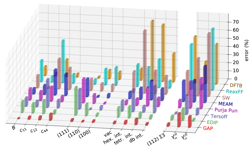
Figure 1 provides an overview of many of the verification and validation tests carried out for our new silicon GAP model in comparison to the empirical analytical models mentioned above. While the individual tests are discussed in more detail below, we present an overview here. The first three groups of quantities in the figure are verification tests, in the sense that they require accuracy on configurations which are directly represented in the training set. These are split into three classes of test: bulk properties, surfaces and point defects. Bulk properties, namely the bulk modulus $B$ and diamond cubic elastic constants $C_{11}$, $C_{12}$ and $C_{44}$, are well reproduced by the GAP model with fractional errors relative to DFT of less than 10%; none of the other interatomic potentials reach this accuracy, although in many cases they were fit to different training data (e.g. experiment, or simply other exchange-correlation functionals). The largest relative errors in bulk properties are typically made in the softest elastic constant $C_{12}$, with the EDIP model being the next most accurate after our new GAP model. The second class of verification tests demonstrates that the GAP model performs consistently at describing surface energies of the $(111)$, $(110)$ and $(100)$ cleavage planes, with errors of around 2% with respect to our reference DFT calculations. Here, the scatter across the various other models is smaller than for bulk properties. For example, the $(100)$ surface energy is in general well described by most models. For the third class of verification tests, formation energies of vacancy and interstitial point defects, we see a wide range of errors across the models evaluated. The new GAP model again predicts all these quantities within 10% of the reference DFT results. In general, for any particular property there is often a model that provides an accurate description but apart from GAP, we are not aware of any model that provides uniform accuracy across the whole range of properties in Fig. 1.

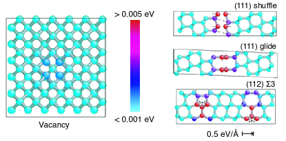
Moving to more stringent tests of the new model, we considered a set of planar defects which were not represented in the training set (right hand group in Fig. 1), namely the $(112)\Sigma 3$ symmetric tilt grain boundary, and unstable stacking fault energies on the $(111)$ shuffle plane $\gamma_{\mathrm{us}}^{(s)}$ and $(111)$ glide plane $\gamma_{\mathrm{us}}^{(g)}$. For these tests the accuracy of the GAP model is reduced, but still within 20% of DFT, comparing favourably with all other models, some of which included stacking fault values in their training sets (e.g. EDIP). Moreover, the ability of the GAP model to provide an estimated error along with its predictions allows us to qualitatively assess the expected reliability of the model for particular classes of configurations. Figure 2 shows the predicted errors for each atom in the vacancy, shuffle, glide and grain boundary configurations. For the vacancy, the confidence of the model is high on all atoms (blue colour), and the corresponding accuracy with respect to DFT is high. The reduced confidence close to the planar defects (red atoms) is consistent with the larger errors made for these configurations and the fact that the database does not include any similar atomic environments.

The rest of the paper is organised as follows. In section II we give an overview of the potential fitting methodology and the construction of the database. In section III we report on extensive tests that serve to verify that those properties which the database is explicitly designed to capture are indeed correctly predicted. This includes equations of state, average structural properties of liquid and amorphous states, point defect energetics, surface reconstructions, and crack tip geometries. In section IV, we validate the model by showing predictions for properties that are deemed fundamental for modeling this material, but for which the database makes no special provision. This includes further crystal structures, thermal expansion, di-interstitials, grain boundaries and random structure search. We finally give a brief outlook in section V.

II Methodology

II.1 Potential fitting

The interatomic potential, even after assuming a finite interaction radius, is a relatively high dimensional function, with dozens of atoms affecting the energy and force on any given atom at the levels of tolerances we are interested in (around a meV/atom). However, much of the interaction energy (in absolute magnitude) is captured by a simple pair potential, describing exchange repulsion of atoms at close approach and potentially the chemical bonding in an average sense farther out. In anticipation of the kernel approach for fitting the interatomic potential, the pair potential also serves a useful purpose from the numerical efficiency point of view, because the exchange repulsion it takes care of is a component of the potential that is very steep, in comparison which the bonding region, and such disparate energy scales are difficult to capture with a single kernel in high dimensions.

In the present case we chose a purely repulsive pair potential, given by cubic splines that were fitted to the interaction of a pair of Si atoms, computed using DFT. This leaves the description of the attractive part entirely for the many-body kernel fit.

We start by giving a concise account of the Gaussian Approximation Potential kernel fitting approach, as we use it here. The total GAP model energy for our system is a sum of the pre-defined pair potential and a many body term which is given by a linear sum over kernel basis functionsRasmussen and Williams (2006),

$$E=\sum_{i<j}V^{(2)}(r_{ij})+\sum_{i}\sum_{s}^{M}\alpha_{s}K({\mathcal{R}}_{i},{\mathcal{R}}_{s}),$$ (1)

where $i$ and $j$ range over the number of atoms in the system, $V^{(2)}$ is the pair potential, $r_{ij}$ is the distance between atoms $i$ and $j$, $K$ is a kernel basis function defined below, and ${\mathcal{R}}_{i}$ is the collection of relative position vectors corresponding to the neighbours of atom $i$ which we call a neighbourhood. The last sum runs over a set of $M$ representative atoms, selected from the input data set, whose environments have been chosen to serve as a basis in which the potential is expanded; more on this below.

The value of the kernel quantifies the similarity between neighbourhoods (in the Gaussian process literature it is a covariance between values of the unknown function at different locations), which is largest when its two arguments are equal, and smallest for maximally different configurations. The degree to which the kernel is able to capture the variation of the energy with neighbour configuration will determine how efficient the above fit is. The better the correspondence, the fewer representative configurations are needed to achieve a given accuracy. It also helps tremendously if exact symmetries of the function to be fitted are already built into the form of the kernel. For an interatomic potential, we need a kernel that is invariant with respect to permutation of like atoms, and 3D rotations of the atomic neighbourhood. Note that translational invariance is already built in, because the kernel fit is applied to each atom individually—this very natural decomposition of the total energy is customary when fitting interatomic potentials, and is directly analogous with the spatial decomposition of convolutional neural networksGoodfellow et al. (2016).

Here we use the SOAP kernelBartók et al. (2013a, b); Bartók and Csányi (2015, 2016). We start by representing the neighbourhood ${\mathcal{R}}_{i}$ of atom $i$ by its neighbour density,

$$\rho_{i}({\bf r})=\sum_{i^{\prime}}f_{\text{cut}}(r_{ii^{\prime}})e^{-({\bf r}-{\bf r}_{ii^{\prime}})/2\sigma^{2}_{\text{atom}}}$$ (2)

where the sum ranges over the neighbours $i^{\prime}$ of atom $i$ (including itself), $f_{\text{cut}}$ is a cutoff function that smoothly goes to zero beyond a cutoff radius $r_{\text{cut}}$, and $\sigma_{\text{atom}}$ is a smearing parameter, typically 0.5 Å. Invariance to rotations is achieved by constructing a Haar integral over the SO(3) rotation groupBartók et al. (2013a, b). The SOAP kernel between two neighbour environments is the integrated overlap of the neighbour densities, squared, and then also integrated over all possible 3D rotations,

$$\tilde{K}({\mathcal{R}}_{i},{\mathcal{R}}_{j})=\int_{\hat{R}\in SO_{3}}d\hat{R}\left|\int d{\bf r}\rho_{i}({\bf r})\rho_{j}(\hat{R}{\bf r})\right|^{2}$$ (3)

To obtain the final kernel, we normalise and raise to a small integer power,

$$K({\mathcal{R}}_{i},{\mathcal{R}}_{j})=\delta^{2}\left|\frac{\tilde{K}({\mathcal{R}}_{i},{\mathcal{R}}_{j})}{\sqrt{\tilde{K}({\mathcal{R}}_{i},{\mathcal{R}}_{i})\tilde{K}({\mathcal{R}}_{j},{\mathcal{R}}_{j})}}\right|^{\zeta}$$ (4)

with $\zeta=4$ in the present case. The $\delta$ hyperparameter corresponds to the energy scale of the many body term, and we use $\delta=3$ eV, commensurate with typical atomization energy/atom. The accuracy of the fit is not particularly sensitive to this parameter.

In practice, we do not evaluate the above integrals directly, but expand the neighbour density in a basis of spherical harmonics $Y_{lm}({\bf\hat{r}})$ and radial functions $g_{n}(r)$ (we use equispaced Gaussians, but the formalism works with any radial basis),

$$\rho_{i}({\bf r})=\sum_{nlm}c^{i}_{nlm}Y_{lm}({\bf\hat{r}})g_{n}(r).$$ (5)

The following spherical power spectrum vector (henceforth termed the “SOAP vector”) is a unique, rotationally and permutationally invariant description of the neighbour environment,

$${\tilde{p}}^{i}_{nn^{\prime}l} =\sum^{l}_{m=-l}c^{i*}_{nlm}c^{i}_{n^{\prime}lm}$$ (6)

$${\bf p}^{i} ={\bf\tilde{p}}^{i}/|{\bf\tilde{p}}^{i}|$$ (7)

and the SOAP kernel can be written as its scalar product,

$$K({\mathcal{R}}_{i},{\mathcal{R}}_{j})=\delta^{2}|{\bf p}^{i}\cdot{\bf p}^{j}|^{\zeta},$$ (8)

The coefficients $\alpha_{s}$ in Eq. 1 are determined by solving a linear system that is obtained when available data are substituted into the equation, as we detail below, as we detail beloww. In the present case these data take the form of total energies and gradients (forces and stresses) corresponding to small and medium sized periodic unit cells, calculated using density functional theory.

We also need an algorithm to select the set of representative environments over which the sum in Eq. 1 is taken. This could be done by simple random sampling, but we find it advantageous to use this freedom to optimise interpolation accuracy. One approach to this is to maximise the dissimilarity between the elements of the representative setDe et al. (2016), such that the small number of environments best represent the variety of the entire set. Here we use a matrix reconstruction technique called CURMahoney and Drineas (2009) and apply it to the rectangular matrix formed by the concatenation of SOAP vectors corresponding to all the neighbour environments appearing in the input data. The CUR decomposition leads to a low rank approximation of the full kernel matrix using only a subset of its rows and columnsImbalzano et al. .

There are two factors that complicate the determination of the vector of linear expansion coefficients, $\boldsymbol{\alpha}$. The first is that atomic energies are not directly available from density functional theory, and the second is the presence of gradients in the input data. The following treatment addresses both of these. We denote the number of atoms in the input database with $N$, and define $\boldsymbol{y}$ as the vector with $D$ components containing the input data: all total energies, forces and virial stress components in the training database, and $\boldsymbol{y}^{\prime}$ as the vector with $N$ components containing the unknown atomic energies of the $N$ atomic environments in the database, and $\mathbf{L}$ as the linear differential operator of size $N\times D$ which connects $\boldsymbol{y}$ with $\boldsymbol{y}^{\prime}$ such that $\boldsymbol{y}=\mathbf{L}{{}^{\mathrm{T}}}\boldsymbol{y}^{\prime}$. After selecting $M$ representative atomic environments (with $M\ll N$), the regularised least-squares solution for the coefficients in Eq. 1 is given bySnelson and Ghahramani (2005); Quinonero-Candela and Rasmussen (2005)

$$\boldsymbol{\alpha}={\big{[}\mathbf{K}_{MM}+\mathbf{K}_{MN}\mathbf{L}\mathbf{\Lambda}^{-1}\mathbf{L}{{}^{\mathrm{T}}}\mathbf{K}_{NM}\big{]}}^{-1}\mathbf{K}_{MN}\mathbf{L}\mathbf{\Lambda}^{-1}\boldsymbol{y},$$ (9)

where $K_{MM}$ is the kernel matrix corresponding to the $M$ representative atomic environments (with matrix elements from Eq. 8), $K_{MN}$ is the kernel matrix corresponding to the representative set and all of the $N$ environments in the training data, and the elements of the diagonal matrix $\mathbf{\Lambda}^{-1}$ represent weights for the input data values. The Bayesian interpretation of the inverse weights are expected errors in the fitted quantities. While taking $\mathbf{\Lambda}=\sigma_{\nu}^{2}\mathbf{I}$ with an empirical value for $\sigma_{\nu}$ would be sufficient to carry out the fit, this interpretation makes it straightforward to set sensible values. The expected errors are not just due to lack of numerical convergence in the electronic structure calculations, but also include the model error of the GAP representation, e.g. due to the finite cutoff of the local environment. Our informed choices for these parameters are reported in Table 1.

For several systems below, we include results on the predicted error, the measure of uncertainty intrinsic to our interpolated potential energy surface. These come from the Bayesian view of the above regression procedure, in which the data (and the predicted values) are viewed as samples from a Gaussian process whose covariance function is the chosen kernel functionRasmussen and Williams (2006). The mean of this Gaussian process is of course just the second term of the predicted energy, Eq. 1, and the predicted variance of the atomic energy for atom $i$ is given by

$$K({\mathcal{R}}_{i},{\mathcal{R}}_{i})-\mathbf{k}^{T}(\mathbf{K}_{MM}+\sigma_{e}\mathbf{I})^{-1}\mathbf{k}$$ (10)

where the element $s$ of the vector $\mathbf{k}$ is given by $K({\mathcal{R}}_{i},{\mathcal{R}}_{s})$, the covariance between the environment of atom $i$ and the environments of the representative atoms $s$ in the database. The above is a simplified error estimate, in which we regularise using the parameter $\sigma_{e}$, typically set to 1 meV (equal to the value used for the per-atom energy data components of $\mathbf{\Lambda}$ for most of the database in Eq. 9), rather than using the more complicated regularisation as in Eq. 9. We interpret this variance as the (square of the) “one sigma” error bar for the atomic energies.

II.2 Database

The database of atomic configurations (periodic unit cells) is described in Table 1. It was built over an extended period, using multiple computational facilities. The kinds of configurations that we included were chosen using intuition and past experience to guide what needs to be included to obtain good coverage pertaining to a range of properties. The number of configuration in the final database is a result of somewhat ad-hoc choices, driven partly by the varying computational cost of the electronic structure calculation, and partly by observed success in predicting properties, signalling sufficient amount of data. Each configuration yields a total energy, six components of the stress tensor and 3 force components for each atom. The database therefore has a total of 531710 pieces of electronic structure data. We represent the diversity of atomic neighbourhoods using $M=9000$ representatives, and the number of these picked from each of the structure types by the CUR algorithm is also shown in the table.

We used the Castep software packageClark et al. (2005) as our density functional theory implementation, and manual cross-checking was done to ensure that the calculations are consistent between different computers. The main parameters of the electronic structure calculation were as follows: PW91Perdew et al. (1992) exchange-correlation functional (the choice was motivated by the existence of large scale simulation of the melting point with this functional), 250 eV plane wave cutoff (with finite basis corrections), Monkhorst-Pack k-point grids with 0.03 Å^-1 spacing, ultrasoft pseudopotentials, and 0.05 eV smearing of the electronic band filling. The remaining numerical error is dominated by the finite k-point grid, leading to errors on the order of a few meVs. The reference data for testing purposes was calculated with the parameters kept the same, except for: bulk energy-volume curves, which used a k-point spacing of 0.015 Å^-1; the re-optimisation of IP minima of amorphous configurations (Table III.3) which used a k-point spacing of 0.07 Å^-1; and molecular dynamics of the liquid, whose parameters are given further below.

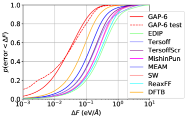
While we focus our efforts here on testing the GAP for its predictions for scientifically interesting observables, we have also evaluated the global distribution of force errors relative to DFT calculations. The results for all the potentials evaluated on the GAP fitting database, as well as for the GAP on a simple testing database (distinct from the fitting database) are shown in Fig. 3. The GAP shows much lower force errors than any other potential tested, with a median of about 0.025 eV/Å, an order of magnitude smaller than for the analytical potentials. The testing database, which consists of a grain boundary, 6 di-interstitials, the unrelaxed and relaxed shuffle and glide generalized stacking fault paths, and an amorphous configuration, shows very similar distribution of force error, although the actual errors are strongly dependent on the type of geometry, so changing the proportions of each could change the resulting distribution somewhat.

Note that the testing database for Fig. 3 is not the result of a usual random split into training and test sets, but represents extrapolation into configurations entirely different from those in the training database. This is a more stringent test than the usual split. Since the empirical analytical potentials have not been fit to our database, the latter serves as a test for the potentials. It is remarkable how good the analytical potentials’ predictions are for macroscopic properties, which are mostly energy differences, given the large force errors shown here.

Figure 3: Cumulative probability distribution of force component errors (relative to reference DFT calculations) for all potentials evaluated on the GAP model fitting database (solid lines), and for the GAP model only on a separate testing database (dashed line).

Structure type	# atoms	# structures	# environments	# representative atoms	$\sigma_{\rm energy}$	$\sigma_{\rm force}$	$\sigma_{\rm virial}$
					default values:
					0.001	0.1	0.05
isolated atom	1	1	1	1
diamond	2	104	208	6
	16	220	3520	53
	54	110	5940	58
	128	55	7040	92
$\beta$-Sn	2	60	120	32
	16	220	3520	51
	54	110	5940	66
	128	55	7040	157
simple hexagonal	1	110	110	13
	8	30	240	15
	27	30	810	42
	64	53	3392	89
hexagonal diamond	4	49	196	7
bcc	2	49	98	40
bc8	8	49	392	66
fcc	4	49	196	46
hcp	2	49	98	28
st12	12	49	588	94
liquid	64	69	4416	1114	0.003	0.15	0.2
	128	7	896	323
amorphous	64	31	1984	231	0.01	0.2	0.4
	216	128	27648	1719
diamond surface (001)	144	29	4176	514
decohesion	32	11	352	28
diamond surface (110)	108	26	2808	338
decohesion	16	11	176	8
diamond surface (111)
decohesion	24	11	264	10
unreconstructed	96	47	4512	573
adatom	146	11	1606	62
Pandey reconstruction	96	50	4800	632
DAS $3\times 3$ unrelaxed	52	1	52	6
diamond vacancy	63	100	6300	168
	215	111	23865	405
diamond divacancy	214	78	16692	416
diamond interstitial	217	115	24955	605
small (110) crack tip	200	7	1400	130
small (111) crack tip	192	10	1920	185
screw dislocation core	144	19	2736	124
sp2 bonded	8	51	408	61
sp bonded	4	100	400	392	0.01	0.2	0.4
Total		2475	171815	9000

Table 1: Summary of the database for the silicon model. The first column shows the number of atoms in the periodic unit cells, the second column shows the number of such unit cells in the database, while the third column is the product of the first two, and thus shows the number of atoms (and therefore atomic environments) in the database for each structure type. The fourth column shows the number of representative atoms picked automatically from each structure type by the CUR algorithm (see text). The last three columns show the regularisation we used in the linear system (empty rows correspond to using the defaults, given at the top).

II.3 Convergence

Since the principal goal of machine learned interatomic potentials is to enable the prediction material properties by fitting the Born-Oppenheimer potential energy surface, it is interesting to consider the convergence of such a potential. The expectation is that a closer match of the potential energy surface will result in more accurate predictions. While a comprehensive convergence study is beyond the scope of this work, there are simple convergence parameters in the SOAP/GAP framework that directly control the tradeoff between computational cost and accuracy of the fit. One is the number $M$ of representative environments (effectively the number of basis functions in the regression), the other is the truncation of the spherical harmonic and radial basis expansion of the atomic neighbour density (Eq. 5).

Figure 4: Error of the SOAP/GAP model based on the $\Delta$-value of Ref. Lejaeghere et al., 2016 with respect to DFT for diamond (black) and $\beta$-Sn (red) structures. The left panel shows the error as a function of the number of basis functions used in the Gaussian process regression. Because we use a stochastic algorithm to select which basis functions to use, multiple models are shown, which only differ in the pseudo-random seed. The right panel shows the error as a function of the length of the SOAP descriptor vector, which in our case is controlled by the truncation of the radial and spherical harmonic expansion of the atomic neighbour density. The horizontal dashed line corresponds to $1$ meV/atom error, our default “energy” accuracy target.

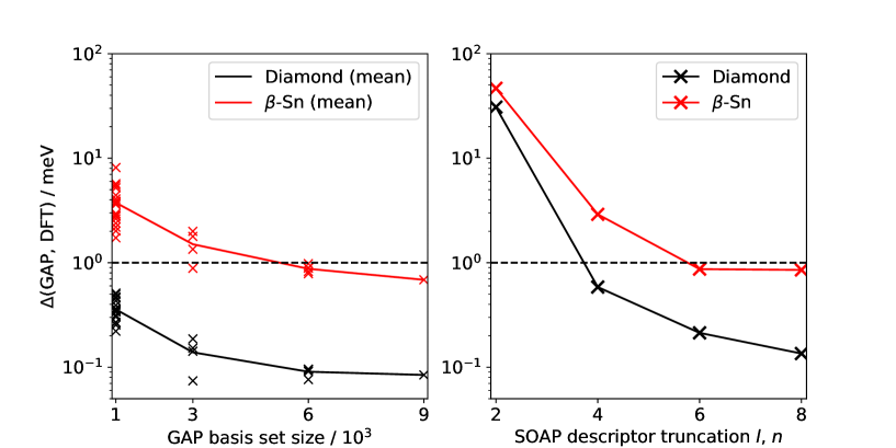
Figure 4 shows the convergence of the SOAP/GAP model with respect to these. We use the $\Delta$-value of Lejaeghere et al. (2016) to compute the error in the energy-volume curves for diamond and $\beta$-Sn with respect to our DFT reference, defined as

$$\Delta=\sqrt{\frac{\int_{0.94V_{0}}^{1.06V_{0}}\left[E^{\mathrm{GAP}}(V)-E^{\mathrm{DFT}}(V)\right]^{2}\,\mathrm{d}V}{0.12V_{0}}}$$

where $E^{\mathrm{GAP}}$ and $E^{\mathrm{DFT}}$ denote GAP and DFT energies relative to the diamond energy minimum to allow comparison, $V_{0}$ is the DFT minimum-energy volume for each phase and the integral is computed numerically by fitting cubic splines to 12 $(E,V)$ pairs for each model. Good convergence can be seen with respect to both basis set size and the accuracy of the expansion of the atomic density, with a precision of the order of a meV (for $\beta$-Sn, for diamond another order of magnitude better), indicating that GAP reproduces the target DFT energy surface better than the typical variability between DFT codes of order $\Delta=1$ meV reported in Ref. Lejaeghere et al., 2016.

In principle, a Gaussian process regression model should be able to converge to a given target function with arbitrary accuracy as the database size grows. However, in this case the only remaining physical approximation is the finite cutoff of the interatomic potential, which means that the force on an atom that is computed using our DFT engine is not strictly a function of the finite neighbourhood of the atom. From the point of view of a model with finite cutoff, the target function appears to have an finite amount of uncertainty, and this uncertainty is taken into account when fitting the model, as mentioned above. Indeed, previous investigations have shown that with a cutoff of 5 Å, an error of 0.1 eV/Å on the forces is about what is to be expected for the diamond structure.Csányi et al. (2005); Bernstein et al. (2009); Peguiron et al. (2015) Note that it is possible to estimate the expected force error due to the finite cutoff directly from the DFT engine because forces are themselves local quantities, as opposed to site energies and virial stress components, which are not observable directly.

It is noteworthy how much more accurate the potential is for the diamond structure than for $\beta$-Sn. Two factors contribute to this: first, there are many more diamond-like configurations in the database, particularly the configurations associated with various defects, and second, the locality error is expected to be significantly larger for the $\beta$-Sn structure due to its metallic electron density of states.

We do not claim that our database in the present work is complete in a mathematical sense (even within the restriction of the given cutoff), but that for any particular application whose relevant configurations are well represented in the database, errors can be improved only by choosing a larger cutoff, which in turn might lead to the need to enlarge the database further.

II.4 Testing

A software testing framework was built to run tests of the potential using the Atomic Simulation Environment (ASE) Larsen et al. (2017). Each model and test is implemented as an independent Python module, allowing all tests to be run with each model (similarly to the design of the OpenKIM project Tadmor et al. (2011)). The model modules are simple, consisting of calls to existing ASE interfaces to QUIP QUI (GAP, DFTB, Stillinger-Weber, Tersoff, and MEAM), LAMMPS lam (EDIP, Purja Pun, and ReaxFF), and Atomistica Ato (TersoffScr). Reference DFT results were obtained using the same tests with a model based on the ASE interface to Castep, and using the parameters discussed above. One advantage of this automated approach is that it ensures consistency in starting configurations, minimization algorithms, and the final test results that are shown in our figures. Another is that it enables automated re-running of tests when changes are made, e.g. to the GAP training database, allowing incremental improvements to be assessed. The framework is available for download.tes

III Results: verification

In this section, we report on a series of basic tests which the GAP model was designed to pass, because they correspond to configurations that were selected for inclusion in the database for the purpose of describing those very observables. We refer to these as “verification”, by analogy to the usage of the term in software engineering, where it refers to confirmation that the software implements the specifications correctly.

It is important to note that by the very nature of such data-driven models, in some sense the database (and the corresponding models) will never be deemed completely final and definitive. By designating some tests as part of “verification,” we mean to be open about the fact that the database was amended qualitatively and quantitatively until these tests were passed to our satisfaction, and therefore these tests are in some sense merely the achievement of a good fit. This is in contrast to the next section, “validation” (again by analogy to the use of the term in software engineering where it refers to confirmation that the specifications describe a method that achieves the desired goal), in which we collect tests for which the database was not explicitly designed, but concern observables that a good model for the material ought to be able to describe. We made no attempt to augment or modify the database in order to improve the results of those tests, and this could, indeed should, be done in future work.

III.1 Bulk crystals

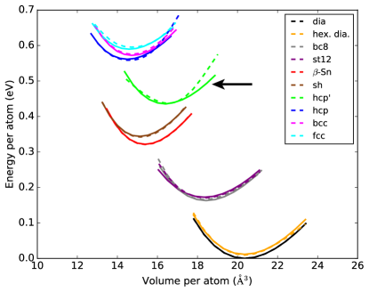
As an initial test we calculated the energy vs. volume for a number of bulk crystal structures for silicon, including the ground state diamond structure, closely related hexagonal diamond, known high pressure structures $\beta$-Sn, simple hexagonal (sh), bc8 and st12 structures, as well as even higher pressure phases, hexagonal close packed (hcp), body centered cubic (bcc), and face centered cubic (fcc). When calculating these curves with DFT as well as DFTB and each interatomic potential we deform the lattice to the target volume and relax it with respect to unit cell shape and atomic position while approximately constraining the volume, and also constraining the symmetry (using spglib spg ) to remain that of the initial structure. We find that the hcp structure has two minima, the conventional one with $c/a\approx\sqrt{3/2}$, and another we label hcp’ which has a much lower $c/a<1$.

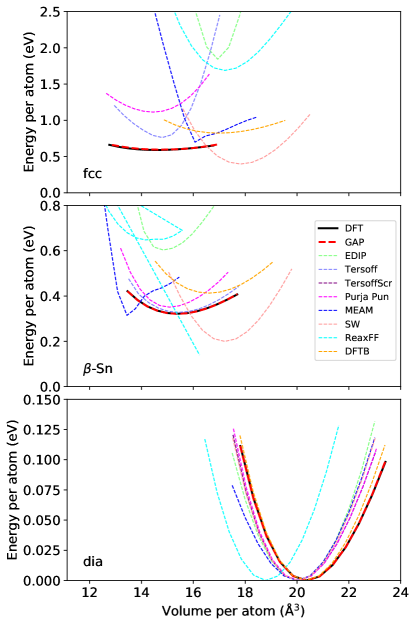
The resulting $E(V)$ curves for each crystal structure calculated with GAP and compared to our reference DFT calculations are shown in Fig. 5. The results are in excellent agreement for all structures tested, including minima positions (volume), depths (cohesive energy relative to the ground state), and curvatures (bulk modulus). The hcp’ structure, which is not in the fitting database, has a larger discrepancy than the other structures, although it is still in good agreement. A comparison of all the models for a few selected crystal lattices (diamond structure, $\beta$-Sn, and fcc), are shown in Fig. 6. Only GAP is even qualitatively reproducing all three selected structures, and many of the models fail to reproduce even the first structure seen experimentally under applied pressure, $\beta$-Sn.

Figure 5: Energy per atom vs. volume per atom for various bulk crystal lattice structures computed using DFT (solid lines) and GAP (dashed lines). The hcp’ structure (indicated by an arrow), which is not in the fitting database, has a substantially larger discrepancy between DFT and GAP than any of the other structures, all of which are in the database.

Figure 6: Energy per atom relative to diamond structure vs. volume per atom for fcc (top panel), $\beta$-Sn (middle panel), and diamond structure (bottom panel), computed with DFT (black, solid line), GAP (red dashed line), and all other models (various colors, dashed lines). Note different y-axis range on each panel.

III.2 Liquid

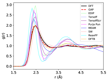
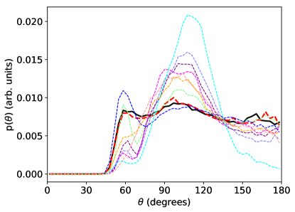
To simulate the structure of liquid silicon with each interatomic potential and DFTB we used constant pressure ($P=0$ GPa) molecular dynamics as implemented in the QUIP package through the quippy Python interface QUI . A $2\times 2\times 2$ supercell of the 8-atom diamond cubic cell (64 atoms total) was heated from $T=0$ K to $T=5000$ K for rapid melting over 20000 0.5 fs time steps, then equilibrated at $T=2000$ K for 10000 0.25 fs time steps. Structural data was gathered over an additional 5000 0.25 fs time steps. Reference DFT results were obtained from a similar MD simulation using the Castep software, averaging over 9700 0.25 fs time steps at $T=2000$ K. For the electronic structure calculations, a 200 eV plane-wave energy cutoff and a $2\times 2\times 2$ Monkhorst-PackMonkhorst and Pack (1976) k-point grid was used (equivalent to a k-point density of about 0.05 Å^-1). The radial distribution function (RDF) and angular distribution function (ADF) were calculated and averaged using the tools included in QUIP.

The resulting structural quantities are shown in Fig. 7. The GAP RDF is in excellent agreement with the DFT result, including both peak heights and radii at all distances captured in the simulation cell. DFTB is in comparably good agreement on this structural quantity, and the various interatomic potentials are in much worse agreement, with signficant variation among them. The ADF proves to be an even more stringent test. Again the GAP results are in excellent agreement with DFT, showing a narrow peak at about 60^∘, and a broader peak with similar height at about 100^∘. Most of the potentials greatly underestimate the height of the small angle peak and overestimate the height of the large angle peak. The only two that are qualitatively correct are EDIP and MEAM, but those both overestimate the depth of the trough separating the two peaks. Several issues with the analytical interatomic potentials may be the source of the differences. Some, for example Tersoff Tersoff (1988a), greatly overestimate the melting point and are therefore strongly undercooled at $T=2000$ K rather than an equilibrium liquid. In other cases it’s possible that the wide variety of curves observed is consistent with the hypothesized liquid-liquid phase transition between a high coordination, high density metallic phase and a low coordination, low density semiconductor-like phase. Ganesh and Widom (2009) Some of the potentials may simply be incorrectly predicting the low coordination phase to be present at $T=2000$ K and zero pressure, leading to a predominantly tetrahedral-like bond angle distribution.

Figure 7: Liquid silicon radial and angular structure from well equilibrated constant temperature and pressure 64 atom samples at $P=0$ GPa and $T=2000$ K. Top: radial distribution function (RDF). Bottom: angular distribution function (ADF). Black solid line indicates DFT results, red dashed line and symbols indicate GAP results, results, and dashed lines (various colours) indicate DFTB and other interatomic potentials.

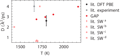
In addition to the two structural quantities we evaluated a dynamical quantity, the diffusivity of liquid Si, by carrying out variable cell size constant enthalpy MD simulations using the LAMMPS software Plimpton (1995); lam on a 512 atom cell for 10⁵ 1 fs time steps at temperatures ranging from about 1700 K to 2200 K. The resulting diffusivity as a function of temperature is shown in Fig. 8, and compared to the experimental results Sanders and Aziz (1999), DFT results Remsing et al. (2017) (using the PBE GGA exchange-correlation functional, which is somewhat different from the PW91 functional we used to generate our fitting database), and previously published SW potential results Broughton and Li (1987); Kakimoto (1998); Yu et al. (1996); Sastry and Angell (2003). The GAP results are in excellent agreement with DFT, and so both underestimate the experimental diffusivity. This difference relative to experiment has previously been ascribed to the tendency for DFT to exaggerate the structure of the liquid, Remsing et al. (2017) and so the similar diffusivities of GAP and DFT are consistent with the similarities in their liquid RDF and ADF.

Figure 8: Diffusivity of liquid silicon from literature DFT simulations Remsing et al. (2017) (black), literature experiment Sanders and Aziz (1999) (grey), GAP (red), and literature SW potential (Refs. Broughton and Li, 1987, Kakimoto, 1998, Yu et al., 1996, and Sastry and Angell, 2003 for $a$-$d$, respectively, pink). Error bars for GAP simulations are smaller than symbols on this scale, and were not available for literature SW results.

III.3 Amorphous phase

Amorphous silicon is an interesting tetrahedrally coordinated phase that forms upon various forms of processing, including ion implantation, low temperature deposition, and rapid quenching from the melt. The last of these is commonly used in simulations, but it is challenging to reach experimentally relevant cooling rates using accurate methods such as DFT. We therefore carried out zero pressure variable cell volume (hydrostatic strain) simulations of the quenching of a 216 atom sample of liquid Si, cooled at 10¹² K/s from 2000 K to 500 K with a 1 fs time step ($1.5\times 10^{6}$ steps) using the LAMMPS software, and then relaxed to the local energy minimum with respect to atomic positions and cell size and shape. The initial configuration for all quenches was from a GAP equilibrated liquid at $T=1800$ K, which was further equilibrated with each potential at $T=2000$ K for an additional 10⁵ time steps before cooling. As for the liquid above, for some potentials this initial thermodynamic state may be a strongly undercooled liquid due to their overestimation of the melting temperature.

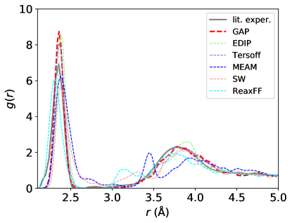
The RDFs of the resulting structures are shown in Fig. 9, in comparison with experimental results Laaziri et al. (1999) (since DFT results for comparable sizes or quench rates are not computationally feasible). The various interatomic models vary widely in the overall shape of their RDF, with GAP, EDIP and Tersoff in best agreement with experiment, showing a sharp first neigbor peak at about 2.35 Å, and a broad second peak at about 3.8 Å. These three models have essentially no atoms between the two peaks ($2.5$ Å $\lesssim r\lesssim 3.25$ Å). The other models show various qualitative problems, including smaller peaks between the two expected ones, or an excess of atoms throughout the entire distance range between the first and second neighbour peaks. The corresponding coordination statistics (using $r=2.75$ Å as the nearest neighbor distance cutoff) are shown in Table III.3. The GAP and Tersoff models have the lowest coordination defect concentration, significantly lower than the next best model, EDIP, and closest to the experimental estimates of $\leq 1$%Nygren and Aziz (1991).

Table III.3 also lists the amorphous-crystal energy difference $\Delta E_{ac}$ relative to the diamond structure. The obvious way to evaluate the energy difference for each structure is to use the same interatomic potential that was used to generate the structure, i.e. a calculation that is entirely self-consistent for that potential. This $\Delta E_{ac}^{\mathrm{IP}}$ listed in the table shows GAP with the closest value to experiment Laaziri et al. (1999) (excluding MEAM, which has a very unphysical structure), while other interatomic potentials result in higher energy differences. However, using the potential to evaluate the energy difference risks mixing up errors in the structure with errors in the energy difference given the structure, with the possibility of exaggerating or understating the stability of the amorphous structure, depending on the sign of the energy error. For an independent evaluation of the quality of the quenched a-Si structures, we evaluated their energies with DFT ($\Delta E_{ac}^{\mathrm{eD}}$), and also further relaxed them with DFT ($\Delta E_{ac}^{\mathrm{rD}}$). Note that these calculations were done with a lower k-point density, 0.07 Å^-1, due to computational expense of the 216 atom cells. In general the unrelaxed DFT energy shows a similar trend to the IP energy, except for SW and MEAM, where the IP energy greatly underestimates the (more reliable) DFT energy difference. Relaxing the structure leads to a small energy reduction for GAP as well as EDIP and Tersoff, indicating a structure that is relatively close to the nearest DFT local minimum, but much larger reductions for the other potentials.

All these DFT results show that quenching a liquid with GAP produces the most stable a-Si structure with the lowest energy difference relative to the diamond structure crystal as compared with the other interatomic potentials, and that the GAP evaluated energy of this structure is in good agreement with DFT. Further work at lower quench rates will be required to generate structures that can be reasonably argued to be directly comparable to experiment.Deringer et al. (2018c)

Figure 9: Radial distribution function (RDF) for 216 atom amorphous configuration generated by cooling at 10¹² K/s from 2000 K to 500 K and then minimized, for GAP (red) and other interatomic potentials (other colors). Experimental results (grey) generated by ion implantation from Ref. Laaziri et al., 1999 are shown for comparison.

Table 2: Coordination statistics $c_{i}$ (fraction of atoms with number of neighbors $i$ within $r_{c}=2.75$ Å, in percent) and energy per atom relative to diamond structure ($\Delta E_{ac}$, in eV) for amorphous structures resulting from quenching of the liquid. Energy difference evaluated using interatomic potential is $\Delta_{ac}^{\mathrm{IP}}$, energy difference of interatomic-potential-relaxed structure evaluated (but not relaxed) using DFT is $\Delta E_{ac}^{\mathrm{eD}}$, and DFT-evaluated energy difference of DFT-relaxed structure starting from interatomic potential structure is $\Delta E_{ac}^{\mathrm{rD}}$. Most atoms in MEAM structure have coordination $\geq 6$. Experimental defect density from Ref. Nygren and Aziz, 1991 and energy from Ref. Roorda et al., 1991.

Model	$c_{3}$	$c_{4}$	$c_{5}$	$\Delta E_{ac}^{\mathrm{IP}}$	$\Delta E_{ac}^{\mathrm{eD}}$	$\Delta E_{ac}^{\mathrm{rD}}$
lit. exper.		$\geq 99$		0.137
GAP	1.4	98.1	0.5	0.15	0.14	0.13
EDIP	0.5	94.4	5.1	0.22	0.22	0.19
Tersoff	0.0	98.1	1.9	0.22	0.18	0.17
MEAM	0.0	0.0	2.8	0.14	0.65	0.28
SW	2.3	75.5	21.8	0.20	0.29	0.23
ReaxFF	0.0	86.1	13.9	0.35	0.35	0.25

III.4 Phase diagram

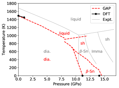
The phase behaviour corresponding to an interatomic potential is a useful benchmark: it not only informs the user about how realistic the model is, but provides an indirect yet stringent test of the microscopic details of the PES. The phase transitions result from a delicate balance between energetic and entropic effects, and for finite temperature transitions probe relatively high-energy configurations. To calculate the liquid-solid transition lines, we performed coexistence simulations for the diamond and simple hexagonal structure at fixed pressure and enthalpy, and measured the resulting average equilibrium temperature. Morris et al. (1994) The diamond/liquid simulations contained 432 atoms and the pressure was fixed at the values of 0, 4 and 8 GPa, and the simple hexagonal/liquid system contained 1024 atoms and the simulations were carried out at 8 and 12 GPa. To estimate the transition line between $\beta$-Sn and simple hexagonal phases, we ran isothermic-isobaric molecular dynamics simulations of both pure phases in a temperature range of 0-1000 K and pressure range of 6-14 GPa, and observed the transition (which occurred in both directions in all cases) by monitoring the Steinhardt bond-order parameters Steinhardt et al. (1983). Finally, the transition line between diamond and $\beta$-Sn structures was determined by calculating the Gibbs free energy using the quasi-harmonic approximation (QHA). We also established that in these phases anharmonic contributions to the free energy differences are negligible at 0 K. We used the LAMMPS package for the MD simulations, and phonopyTogo and Tanaka (2015) for the phonon calculations. Figure 10 shows the calculated phase diagram, compared to the published DFT results for the diamond/liquid melting pointAlfè and Gillan (2003) and our own calculations with the Castep program for the diamond/$\beta$-tin and $\beta$-tin/simple hexagonal transition pressures at 0 K. For comparison, we also show the experimentally determined phase relationsVoronin et al. (2003). Note that the Imma phase is missing from the calculated phase diagram. This is due to the fact that both our DFT calculations and GAP model find the Imma phase to be metastable.

Figure 10: Temperature-pressure phase diagram of silicon, computed with GAP (red), compared to available DFT results (black) and experimental phase transitions (grey). The finite temperature DFT result is from Ref. Alfè and Gillan, 2003, and the experimental lines are from Ref. Voronin et al., 2003.

III.5 Defects

III.5.1 Point defects

Several point defects were represented in the fitting database (Table 1), and their formation energies would therefore be expected to be accurately reproduced by the GAP. Indeed, as Fig. 1 shows, the relative error for the vacancy and three interstitial positions, hexagonal, tetrahedral, and dumbbell, are all within at most 7% of the reference DFT values. The only other potential that is close to this level of accuracy is EDIP, with similar errors for all but the hexagonal interstitial, where it is off by 14%. All the other potentials, as well as DFTB, differ from our DFT calculations by tens of percent for at least some of the defects.

Since point defects control properties such as diffusivity in bulk silicon, their migration barriers are also of interest, and as they represent bond breaking and formation processes, often present a challenge for interatomic potentials. Since the training database configurations came from finite temperature MD, it could in principle include configurations near the barrier, but since the system spends relatively little time near the energy saddle point this is actually unlikely Li et al. (2017b). However, the hexagonal and tetrahedral interstitials are related by a short displacement, so one is typically a local minimum and the other a saddle point along an interstitial diffusion pathway. We find that GAP preserves the DFT ordering, although the energy difference is underestimated, while the other potentials make much larger errors, many reversing the relative order of the two high symmetry geometries. Two other related observables, the migration path of the vacancy and the formation energy of the four-fold defect (the midpoint of the concerted-exchange diffusion mechanism Pandey (1986); Kaxiras and Pandey (1993)), which are not represented in the database, are discussed below in Sec. IV.5 and Sec. IV.6.

III.5.2 Surfaces

Surfaces are a class of defects that have particular importance for the behaviour of materials. Solids fail under tension by opening new surfaces, and it is on surfaces that reactions involving chemical species in the environment can take place, where special functional layers can form e.g. by oxidation, and also where a crystal can grow under suitable conditions. Apart from useful applications, a rich complexity of bonding emerges on surfaces due to the subtle interplay of strain effects with the chemistry of dangling bonds. This makes surface formation energies, and particularly the energies and geometries of various reconstructions, a sensitive test of the accuracy of an interatomic potential.

Figure 11: Decohesion energy of diamond-structure silicon along various directions (labelled according to the orientation of the opening surface). Insets (same axes as main plot) show errors with respect to DFT for the current GAP (red) as well as for a previous version of the GAP (grey) with a fitting database that did not include any configurations along the separation path (or high energy crystal-lattice structures), but only final fully seprated surfaces.

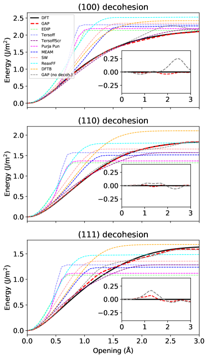
Figure 11 shows the energy as a function of separation as a gap is opened up in a unit cell that is long in one direction and has the dimensions of the minimal surface unit cell in the orthogonal plane. For the purposes of this test, the atomic positions were not relaxed, but kept rigid relative to one another as the gap was opened. All analytical potentials apart from the screened Tersoff show far too short a range - they plateau much earlier than DFT, and in fact this was one of the motivating factors behind modifying the original Tersoff potentialPastewka et al. (2008, 2013). The right hand side limit corresponds to the unrelaxed surface energy in each case, a property in which the potentials show about 30% scatter. Note that in the case of the $(111)$ surface, DFT is believed to overestimate the surface energyJaccodine (1963) and, e.g., Tersoff and its screened version were explicitly fit to reproduce the experimental value.

Note that the final version of the fitting database for the GAP presented here includes configurations along the separation path, in addition to fully separated surfaces. An earlier version of the GAP model Bartók et al. (2017a) that did not include configurations from the separation path correctly reproduced the fully separated energy (since fully separated surfaces were included in the fitting), but not the intermediate energies, as shown in the insets in Fig. 11. The test results for the version of the potential without the decohesion path configurations (as well as fewer non-diamond crystal structures), listed in detail in the Supplemental Informationsup , were very close to the final GAP values, with most tested quantities differing by less than 1%. The only exceptions were the quantities directly related to configurations newly added to the database, and a few other tests (described later in this subsection and in Section. IV.7) that were not explicitly fit (two di-interstitial formation energies that changed by 3% and 10%, and the (111) reconstructed surface energies that changed by 2%-3%). This example shows that the flexibility of the GAP functional form makes it possible to correct shortcomings by adding configurations to the database without significantly affecting accuracy for other configurations.

Figure 12: Geometry of the 2x1 reconstruction of the (100) surface, showing the tilting of the surface dimers. The dashed circles show the surface dimer in the untilted (but rebonded) position.

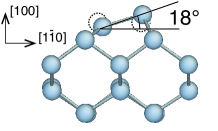
Figure 12 shows the geometry of the tilted-dimer $2\times 1$ reconstruction, one of the low energy configurations of the (100) surface, which forms spontaneously from the as-cut surface. In this reconstruction the surface atoms dimerize to form additional bonds, and the dimers tilt (by $18^{\circ}$ in our DFT calculations) due to a Jahn-Teller effectHaneman (1987), which would seem to require an explicit description of the electrons. In fact, none of the analytical potentials reproduce the substantial tilting (zero tilt for all but EDIP, which tilts by $4^{\circ}$). Only GAP, with its relatively long range and flexible form, captures the tilting in reasonable agreement with DFT (-$2.5^{\circ}$ error). The DFTB model, with its minimal description of electronic structure also shows the breaking of symmetry with a similar error on the resulting bond angle of about -$2.3^{\circ}$.

Figure 13: Formation energy of the dimer-adatom-stacking-fault (DAS) reconstruction of the (111) surface for various surface unit cell sizes $n=(3,5,7,9)$ computed with different models. The value shown at $n=1$ corresponds not to a DAS reconstruction, but rather the unreconstructed surface. The box on the lower right is a magnified view that shows just the DFT and GAP results.

Figure 14: Two views of the DAS $3\times 3$ (111) surface reconstruction configuration that is in the database with atoms, marked with dark grey, whose environments were selected to be amongst representative set for the purposes of defining the GAP model.

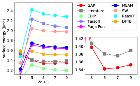
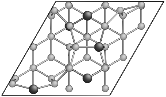
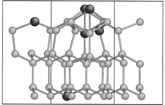
The lowest energy configuration of the $(111)$ surface is the famous $7\times 7$ dimer-adatom-stacking-fault (DAS) reconstruction, already alluded to in the introduction. It is a rather complex structure, involving a 2D super-lattice of 10-atom rings, connected by dimerized dislocation cores that separating triangles of stacking faults, half of which have extra atoms on top. A family of analogous structures can be defined by varying the number of dimers, $n\geq 3$, between the vertices of the super-lattice, leading to the designation $(2n+1)\times(2n+1)$. As shown in Fig. 13, all analytical potentials predict these reconstructions to be higher in energy than the unreconstructed surface (shown in place of $n=1$ for simplicity), and furthermore, within the family of DAS structures, the energy goes down as $n$ goes up. Computing accurate DFT energies is a nontrivial calculation, and its prediction that the $7\times 7$ DAS structure is the lowest energy configuration was a significant early triumph of DFT Štich et al. (1992). Here our reference is a more recent careful determination of the DFT energiesSolares et al. (2005). The DFTB model again stands out as qualitatively different from the analytical models, but still failing to show quantitative agreement with DFT. The GAP model, which includes in its training database just a single configuration of the $3\times 3$ DAS structure (shown in Fig. 14), gives energies with error below 0.05 J/m² (much smaller than a meV/atom over the supercell), correctly predicting the DAS family to be lower in energy than the unreconstructed surface, and also giving an energy minimum.

The lowest energy structure for the present potential happens to be for $n=5$, within 0.01 J/m² of the $7\times 7$ structure. The energy differences are much smaller than the target (and assumed) error in the GAP model, and as such this level of detail is not robust: the earlier variant of the potential fitted to a slightly different database (in ways unrelated to the (111) surface) show the $7\times 7$ DAS structure as the global minimum, as shown beforeBartók et al. (2017b). What is robust is the relationship of the energies of the DAS family to other types of reconstructions, and the upturn in energy for $n=9$. Significantly more data relevant to these structures would be needed in order to robustly capture the finest of relative energies within the DAS family.

Figure 14 shows which atoms were picked (automatically, by the CUR decomposition of the descriptor matrix, as mentioned above) to be part of the representative set: mostly those that are unique to the DAS family of reconstruction and do not appear elsewhere in the dataset, i.e. the adatom, the atom just below it, one of the dimer atoms in at the boundary of the stacking fault, and one atom on the 10-ring that surrounds the vertices of the surface unit cell.

III.6 Crack Propagation

The atomic-scale details of crack propagation have proved particularily challenging to model, since sufficent accuracy to describe bond breaking processes must be combined with large model systems to avoid unrealistic strain gradients Bitzek et al. (2015). Interatomic potentials which provide an otherwise good description of the bulk and elastic properties of silicon (e.g. the Stillinger-Weber and Tersoff potentials) tend to overestimate the lattice trapping barriers to brittle fracture, resulting in an overestimate of the fracture toughness as well as an erroneously ductile material response including features such as crack arrest and dislocation emission Swadener et al. (2002); Holland and Marder (1998a, b). Progress has been made using reactive potentials such as ReaxFF Buehler et al. (2006) or with hybrid quantum/classical approaches where an ab initio crack tip model is embedded within a larger classical model system Bernstein and Hess (2003b); Kermode et al. (2008b); Gleizer et al. (2014). The latter limits the applicability to timescales accessible to DFT, making it extremely challenging to study processes such as thermally activated crack growth Kermode et al. (2015).

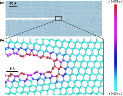
To test the accuracy of our new GAP model for fracture, we considered the well studied $(111)[1\bar{1}0]$ cleavage system, where fracture is known to exhibit a low speed instability triggered by the formation of a crack tip reconstruction Kermode et al. (2008b). We performed simulations of a 23,496 atom model system of dimensions $600\times 200\times 3.86$ Å³ using both molecular dynamics at 300 K with a range of strain rates between $10^{-6}$ and $10^{-4}$ fs^-1, and quasi-static strain increments followed by relaxation. In all cases the trajectories obtained were consistent with those expected from our earlier DFT-based hybrid simulations as reported in Ref. Kermode et al., 2008b. The GAP model predicts brittle fracture morphology with an atomically smooth fracture surface and the occasional formation of crack tip reconstruction and subsequent surface steps in the ‘downward’ $[111]$ direction, in line with the results of our previous study. A snapshot from a quasi-static simulation showing the formation of the crack tip reconstruction at a strain energy release rate of $G=5.13$ J/m² is illustrated in Fig. 15. The atoms are coloured by the predicted error of the GAP model, showing high confidence in the bulk and with larger predicted errors at the crack tip; nevertheless, qualitatively correct surfaces and crack tip reconstructions are obtained.

Figure 15: (a) Snapshot from a quasi-static simulation of fracture in the Si$(111)[1\bar{1}0]$ cleavage system at a strain energy release rate of $G=5.13$ J/m². Model system contains 23,496 atoms and has dimensions $600\times 200\times 3.86$ Å³. (b) Close up of the crack tip, which has undergone a crack tip reconstruction as previously reported in DFT-based hybrid simulations in Ref. Kermode et al., 2008b. Atoms are coloured by the predicted error per atom of the GAP model, from blue (low) to red (high).

IV Results: Validation

In addition to the tests presented in the previous section, we tested quantities and configurations that are physically important but do not map so cleanly to particular geometries in the database. The first is random structure seach, which probes a very wide range of geometries, bonding topologies, and energies. The second is a test of the vibrational properties (harmonic phonons and anhramonic Grüneisen parameters) of the diamond structure, which are only implicitly included in the fit through the perturbed diamond configurations. Finally two types of defects were tested, a high-symmetry grain boundary and di-interstitials, which have geometries related to, but clearly different than, the defects in the fitting database.

IV.1 Random structure search

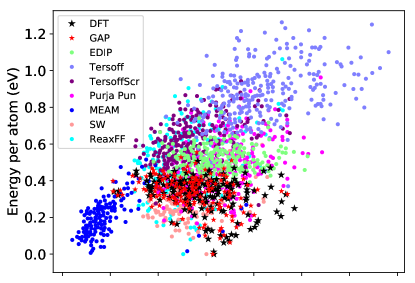
The random structure search Pickard and Needs (2006, 2011) (RSS) method provides a global test of the potential energy surface, including not only regions near the physically reasonable minima (i.e. typical bulk lattices with small distortions and defects that vary only locally from the bulk structure), but also much more distorted and correspondingly higher energy configurations. We carried out RSS using the various interatomic potentials and DFT for 8 atom unit cells with constraints on the initial shape (close to cubic) and interatomic distances ($>1.7$ Å) to exclude unphysically close atoms, relaxed with the two-point steepest descent Barzilai and Borwein (1988) method. The resulting distribution of configuration energy and volume are plotted in Fig. 16. The GAP results show a similar distribution to DFT, with the diamond structure at the correct volume, a few structures with energies up to 0.2 eV/atom higher, mostly at comparable or somewhat larger volumes (with one or two exceptions at substantially smaller volume), and a large group at more than 0.2 eV/atom higher at comparable or smaller volume. None of the interatomic potentials give a similar distribution, and some of the more sophisticated ones give drastically different distributions, including low energies for extremely small (25% below diamond structure) volumes, or unphysical local minima at very high energies ($>0.4$ eV/atom).

Figure 16: Relaxed volumes and energies (relative to diamond structure) for random structure searches. Top panel shows scatterplot with DFT (black stars), GAP (red stars), and various other interatomic potentials (various color circles). Bottom panel shows convex hull surrounding all minima for each method with same x-axis and colors as top panel.

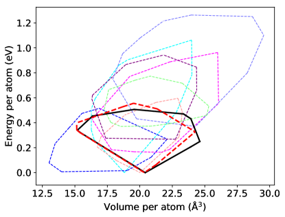
While the distribution of energies and volumes for the GAP relaxed minima is similar to that of the DFT relaxed ones, that does not necessarily mean that individual minima predicted by GAP are also DFT minima. To test this, we further relaxed the GAP minima using DFT, and plotted the resulting positions on the (E,V) plane in Fig. 17. The plot shows that in many, although clearly not all, cases the GAP energy for GAP minimum configurations is close to the DFT energy for the same configuration, and further relaxation with DFT does not change the volume or energy very much. The distribution of volume changes, shown in Fig. 18, confirms that most volume changes are small, with 80% falling below 1 Å³/atom, or about 5% of the diamond structure volume.

Figure 17: Energies and volumes of relaxation of GAP RSS minima with DFT forces and stresses. Red circles indicate GAP minima, grey circles indicate DFT energies of GAP minima configurations, and black circles indicate energy and volume of DFT relaxed configurations starting from the corresponding GAP minimum.

Figure 18: Distribution of volume changes for relaxation of GAP minima using DFT. Dotted vertical line indicates the 80’th percentile. Inset shows energy per atom for trajectories generated by DFT relaxation starting from GAP RSS minimum, computed with DFT (black solid line) and GAP (red dashed line), for one configuration with a small volume change and one with a large volume change.

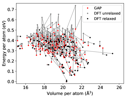
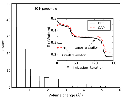
A better understanding of the large volume changes that sometimes occur during DFT relaxation comes from calculating the GAP energy for the DFT relaxation trajectory configurations. Two examples of these energy variations are shown in the inset of Fig. 18. For the configuration with a small overall volume change, the DFT energy goes down a bit and quickly flattens as the DFT minimum is reached, while the GAP energy on the same trajectory goes up a bit (as it must, since the initial configuration is a GAP local minimum), and also flattens. On the other hand, for the configuration with the large volume change, the DFT energy does not flatten immediately, but instead goes through a sequence of drops and flat regions as it explores various near minima on the PES. While the initial GAP local minimum is not also a DFT local minimum, the barrier that separates it from other minima on the GAP PES is small, and all of the configurations that the DFT minimization trajectory goes through have very similar energies (within 0.05 eV/atom) with DFT and GAP. This shows that while the GAP PES is not perfect, differing in the positions and height of some small energy barriers, the overall shape of the PES is in fact in good agreement with DFT.

IV.2 Phonons and thermal expansion

Vibrational properties probe the PES in the region close to the minima, and influence the thermodynamic and transport behaviour of the material. We computed the phonon and mode Grüneisen dispersion curves in the cubic diamond structure with GAP, DFT, DFTB and various interatomic potentials using phonopyTogo and Tanaka (2015). The results are shown in Fig. 19. Even though the phonon frequencies were not included in the database explicitly, there is an excellent agreement between DFT and GAP. The analytical interatomic potentials are generally in good qualitative agreement for the phonon spectrum, although they overestimate the acoustic branch zone-edge and all optical branch frequencies, while DFTB is in significantly better agreement with DFT. Not unexpectedly, the slope of the dispersion curves at small k-vectors is well reproduced, corresponding to the generally good agreement of the elastic constants of the examined potentials with DFT. GAP Results for the mode Grüneisen parameter are more mixed, with the transverse acoustic branch showing a large discrepancy, indicating that the force data of near-equilibrium crystalline configurations is not sufficient for the fitting procedure to resolve the anharmonicity of the PES. The analytical potentials and DFTB, on the other hand, differ qualitatively from the DFT calculation for all branches.

Figure 19: Top panel: phonon dispersion curves of cubic diamond silicon at 0 GPa with various models. Bottom panel: dispersion curves of mode Grüneisen parameters.

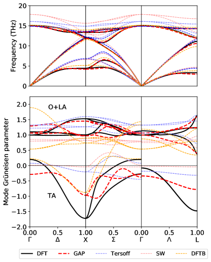
Diamond structure silicon displays negative thermal expansion at low temperaturesOkada and Tokumaru (1984) due to phonon entropic effects, and this behavior is reproduced by DFTBiernacki and Scheffler (1989). To benchmark this unusual feature and other thermal properties of GAP, we calculated the thermal expansion and Grüneisen parameters using QHA and the heat capacity from the phonon frequenciesMounet and Marzari (2005). Figure 20 shows the temperature dependence of the linear thermal expansion, the Grüneisen parameter and the heat capacity of various models including GAP and DFT. Even though the mode Grüneisen parameters of DFT are not accurately reproduced by GAP, these averaged thermodynamic properties show a reasonable agreement, including the temperature region with negative thermal expansion. Analytic potentials and DFTB show a good agreement in the temperature dependence of the heat capacity, not surprisingly, as phonon frequencies are generally similar. However, the errors that the other tested models made in the mode Grüneisen parameters shown in the previous figures manifest themselves here in the form of qualitative errors in the thermal expansion, where none reproduce the negative values at low temperature. At small temperatures, mostly low energy states are excited, and in particular, those in the transverse acoustical (TA) branch. The hardening of phonons, or in other words, the strongly negative mode Grüneisen paramters, in the TA branch have been associated with the negative thermal expansion of silicon Biernacki and Scheffler (1989). The shift to large positive values of the TA mode Grüneisen parameters of DFTB in the $\Lambda$ direction is probably the reason for the spurious maximum in the Grüneisen parameter.

Figure 20: Linear thermal expansion, Grüneisen parameter, and specific heat of silicon computed with various models, using the quasi-harmonic approximation, compared to experimental results: a: Lyon et alLyon et al. (1977) b: Okada and TokumaruOkada and Tokumaru (1984).

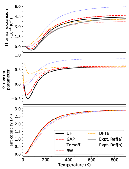
IV.3 Generalized stacking faults

One type of planar defect that is important as a representative of dislocation properties which control macroscopic behavior such as plasticity and fracture, is the generalized stacking fault (GSF) surface Vitek (1968). This generalization of the conventional stacking fault, which has been studied extensively in silicon Kaxiras and Duesbery (1993); Juan and Kaxiras (1996); de Koning et al. (1998); Godet et al. (2003), is the energy as a function of arbitrary in-plane shift between two blocks of otherwise undisturbed crystal. We focus on the diamond structure $(111)$ planes, where the GSF can be introduced in glide planes (within a bilayer) or shuffle planes (between bilayers). We calculated the energy along high symmetry paths on the GSF surface connecting equivalent representations of the ideal crystal in a $1\times 1$ $(111)$ surface cell with 9 bilayers (18 atoms) in the normal direction, relaxing the atoms parallel to the surface normal. In each case we chose the minimum barrier energy path, $[112]$ for the glide fault and $[110]$ for the shuffle fault. The resulting energies along the paths for GAP and the reference DFT results are shown in Fig. 21. For both relaxed shuffle and glide GSFs the GAP results are in good agreement with DFT. The predicted errors shown in the plot are significant near the peaks of both paths, consistent with a relatively large disagreement with the DFT reference values, and with the fact that neither type of configuration was included in the fitting database.

A comparison of the energy along one of the paths, glide plane relaxed, for all potentials, is shown in Fig. 22, and the corresponding fractional errors in the peak energy along all relaxed paths relative to DFT for all the interatomic potentials are shown in Fig. 1. The results for GAP show reasonable agreement with DFT, similar to the best of the other interatomic potentials, and much better than most.

Figure 21: Relaxed generalized stacking fault energies along minimum barrier energy path directions ($[112]$ for glide and $[110]$ for shuffle) computed with DFT (black solid lines) and GAP. The thick curve showing the GAP model energies is coloured according to the maximum per-atom predicted error of the GAP model, and dashed where the predicted error exceeds the scale maximum of 5 meV/atom. The upper two curves correspond to glide plane and the lower two to the shuffle plane.

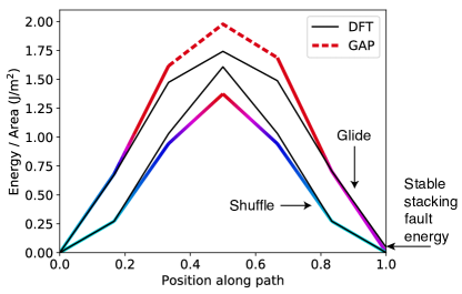
The final point on the glide plane GSF path is the conventional stable stacking fault energy $\gamma_{\mathrm{sf}}$, which is listed in Table 3. The DFT reference value is small and positive, indicating that the hexagonal stacking is higher in energy than cubic diamond structure. To get a sense of the scale, note that the glide curve does not quite reach zero at the right hand side of Fig. 21: that mismatch corresponds to the stable stacking fault energy. The GAP value is positive but much too small, indicating that diamond structure is indeed the lowest energy configuration, but underestimating the energy difference. There are four atoms with non-diamond-like second neighbour environment, and the DFT energy difference corresponds to a contribution of about 10 meV from each roughly in correspondence with the $\sim\!2.5$ meV/atom predicted error (purple colour). The elevated predicted error shows that GAP’s range and flexibility can distinguish these environments, and the $\gamma_{\mathrm{sf}}$ value could probably be improved by extending the database. While most potentials tested are short ranged and give exactly zero energy, ReaxFF has a similar value to GAP, while MEAM gives a qualitatively incorrect negative $\gamma_{\mathrm{sf}}$. The DFTB model is the only one that accurately reproduces the DFT value.

Table 3: Stable stacking fault energy $\gamma_{\mathrm{sf}}$ for each model.

Model	$\gamma_{\mathrm{sf}}$ (J/m2)
DFT	0.047
GAP	0.002
EDIP	0.000
Tersoff	0.000
TersoffScr	0.001
Purja Pun	0.000
MEAM	-0.046
SW	0.000
ReaxFF	0.004
DFTB	0.052

Figure 22: Relaxed glide-plane generalized stacking fault energies along minimum barrier energy path $[112]$ direction computed with DFT (solid lines), GAP (red dashed lines with symbols), and other interatomic potentials (other color dashed lines).

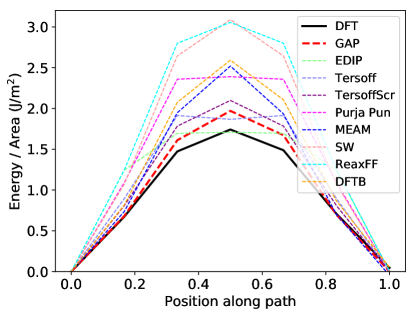
IV.4 Grain boundary

Another class of planar defects that was not included in the fitting database are grain boundaries, which are the interfaces between identical crystal lattices in different orientations. As a simple example of these structures we chose the $(112)~{}\Sigma 3$ tilt boundary of the diamond structure, which can be represented by a relatively small unit cell and can therefore be efficiently computed with DFT. We computed the energy per unit area of this grain boundary with the various interatomic potentials and DFTB, as well as DFT, using a cell with 48 atoms, which had a single interface unit cell and was about 27 Å long normal to the boundary. The resulting fractional errors relative to the DFT value are shown in Fig. 1, and the GAP force errors for the DFT relaxed configuration are shown in Fig. 2. Despite the fact that the grain boundary structure was not in the fitting database, the GAP energy is in excellent agreement with DFT. The difference between the DFT and GAP relaxed geometries is also small, as indicated by the small magnitudes of the GAP forces in the DFT relaxed geometry (Fig. 2), and the corresponding displacements (not shown) are nearly imperceptible. The accuracy of the other interatomic potentials varies considerably, with some also in very good agreement but others with very large energy errors relative to the DFT reference.

IV.5 Four-fold defect

The point defect with the lowest formation energy in the diamond structure of silicon is the so-called “four-fold coordinated defect”Goedecker et al. (2002), which is formed by a bond rotation followed by reconnecting all broken bonds. The energy barrier for the reverse process (i.e. annealing out this defect) is relatively small, and the GAP model does not in fact stabilise this defect, as shown in Fig. 23. Indeed, the database does not contain anything resembling the bond rotation process or the final defect structure, and this is quantitatively shown by the predicted error. The energies of the GAP model agree very well with those of DFT up to where the predicted error (taken as the maximum over all atoms) is lower than about 3 meV/atom, and strongly deviate after that. Similarly to the planar defects, the predicted error gives a good qualitative indication of where the database is deficient and is in need of extension.

Figure 23: Relaxation path of the GAP model showing the instability of the four-fold defect. The left hand side of the plot corresponds to the local minimum of the four-fold defect for the DFT model. The black curve shows the energy of the configurations of this path evaluated with DFT (this is not a DFT minimum energy path, but of course still shows a barrier). The thick curve shows the GAP model energies, coloured according to the maximum per-atom predicted error of the GAP model, and is dashed where the predicted error exceeds the scale maximum of 5 meV/atom.

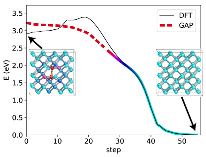
IV.6 Vacancy migration

We compared the migration paths for vacancies in 63 atom diamond structure cells predicted by the various models, as a test of their ability to describe bond breaking processes. The endpoints were relaxed with preconditioned LBFGSPackwood et al. (2016) to a maximum force tolerance of $10^{-3}$ eV/Å, and the path was calculated as a linear interpolation between the two relaxed endpoints. The intermediate configurations were not relaxed (as in, for example, the nudged elastic band methodHenkelman and Jónsson (2000)), because features in the PES of many of the potentials led to ill-behaved paths, similar to the inconsistencies previously noted for the Tersoff potential Posselt et al. (2008). The results shown in Fig. 24 indicate the wide variability in the quality of the predictions from the interatomic potentials in comparison to DFT, with many of the models significantly over or underestimating both the formation energy and the migration barrier for vacancies.

For GAP, MEAM and TersoffScr, which produce formation energies and barriers close to DFT, the minimum energy path (MEP) was determined using the nudged elastic band (NEB)Henkelman and Jónsson (2000) algorithm as implemented in ASE using 9 intermediate images between minima. The results shown in Fig. 25 show that GAP produces the most accurate MEP in comparison to DFT, albeit with an underestimate of the barrier. TersoffScr predicts a local minimum at the split vacancy configuration. The insets show the per-atom GAP predicted errors at one of the minima and close to the saddle point; the model is more confident near the minima since it has been trained on similar configurations, while saddle-like configurations were not present in the training data. The predicted error here again provides a useful guide to the expected reliability of the model, with good agreement with DFT where it is low and decreasing agreement where it exceeds 3 meV per atom.

Figure 24: Unrelaxed energy profiles for the migration of a vacancy, consisting of a series of linearly interpolated configurations between relaxed vacancy endpoints, in a 63 atom diamond cell for all models. Energies are calculated relative to a bulk crystal with the same number of atoms so that the endpoints indicate the relaxed vacancy formation energy.

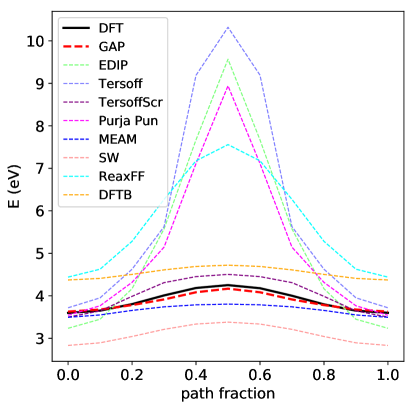
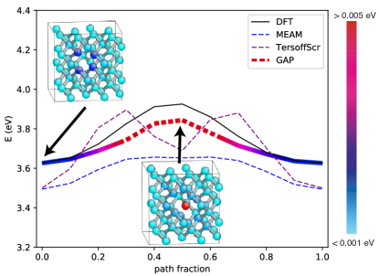
Model	Formation / eV	Error	Barrier / eV	Error
DFT	3.63	—	0.30	—
MEAM	3.49	-3.7%	0.16	-45.6%
TersoffScr	3.50	-3.5%	0.40	32.5%
GAP	3.63	-0.0%	0.22	-27.0%

Figure 25: Comparison of DFT, GAP, MEAM and TersoffScr models for the migration of a vacancy. Lines show NEB minimum energy pathways for a 63 atom cell, with the thick GAP line and inset images coloured by the predicted error, becoming dashed where the maximum error exceeds 0.005 eV/Å, showing the model is more confident at the minima than the saddle.

IV.7 Di-interstitials

Although configurations including simple point defects, such as the mono-vacancy and the interstitial were part of our training database, the di-interstitial provides an interesting test case of transferability to new defect types. The atomic neighbour environments involved in the di-interstitial are clearly different from anything that was explicitly included in the database. Figure 26 shows the percentage error that various interatomic potentials make in the formation energy of the diinterstital for six different conformations. We used 66 atoms in the unit cell, including the two extra that were added to a conventional 64 atom cubic unit cell. The starting positionsBorodin and Ganchenkova were relaxed with each potential, as well as DFT, and the final energies from each local minima compared.

The results show that most potentials struggle with this property. EDIP for example, which performs relatively well for the mono-vacancy and the single interstitial makes up to 20% error here. The Stillinger-Weber model on the other hand, which made errors of over 50% for the single point defects, looks rather better here. MEAM, ReaxFF and DFTB perform poorly, similarly to the case of single point defects. It is also clear from the plot, that all potentials struggle with the TT configuration (even the best result is over 10%), including GAP (which otherwise has errors less than about 6%). Figure 27 shows the corresponding relaxed geometries using the GAP and Stillinger-Weber model, as well as DFT, with coloured markings for significant deviations. The Stillinger-Weber model, despite its competitive energy accuracy, shows many more distorted geometries.

Figure 26: Percentage error in the formation energy of di-interstitials (I₂) in various configurations for a variety of interatomic potentials, relative to DFT.

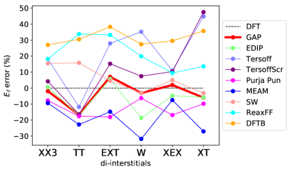
GAP
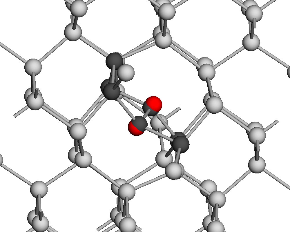
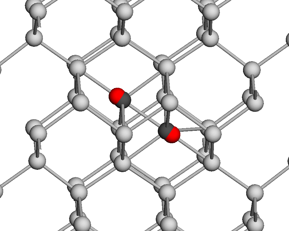
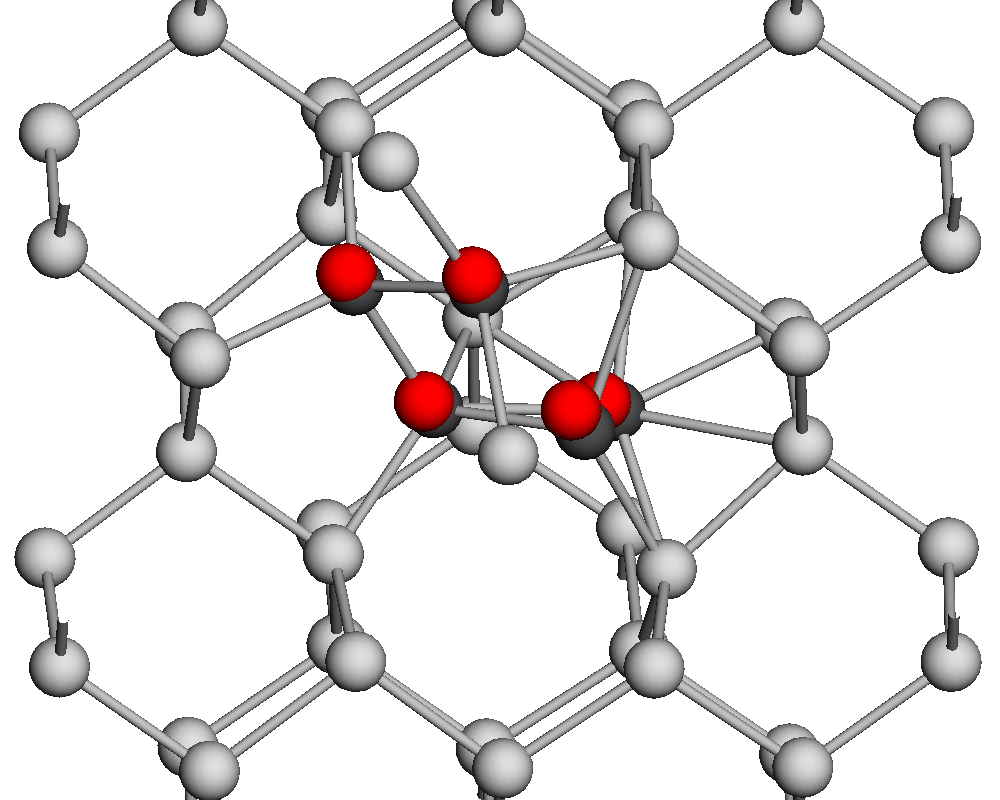
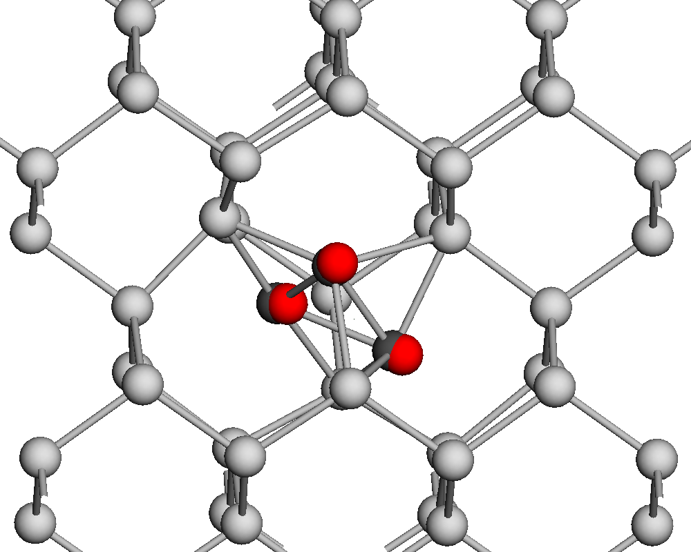
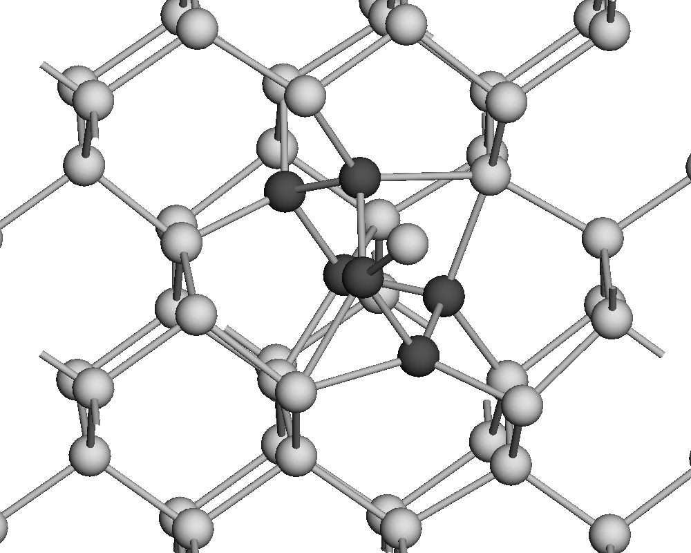
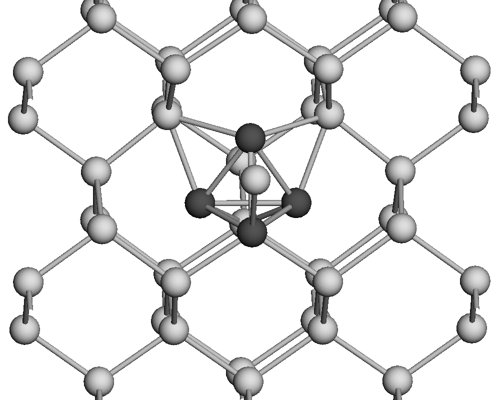
SW
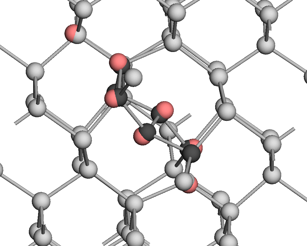
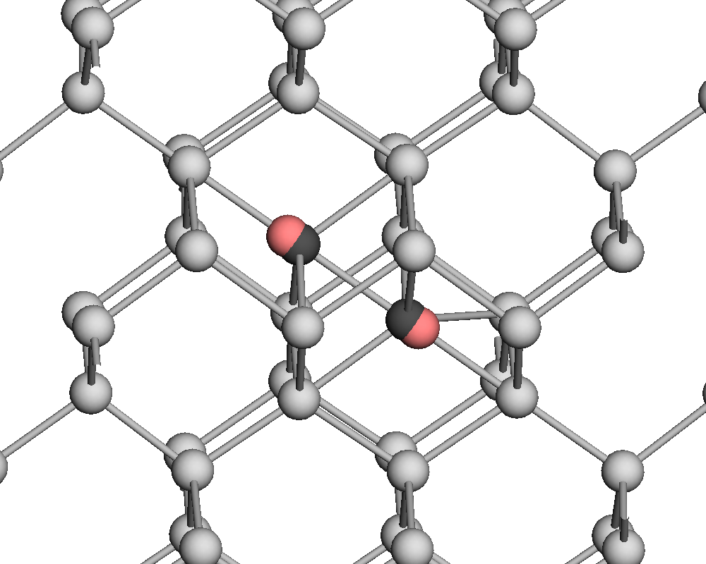
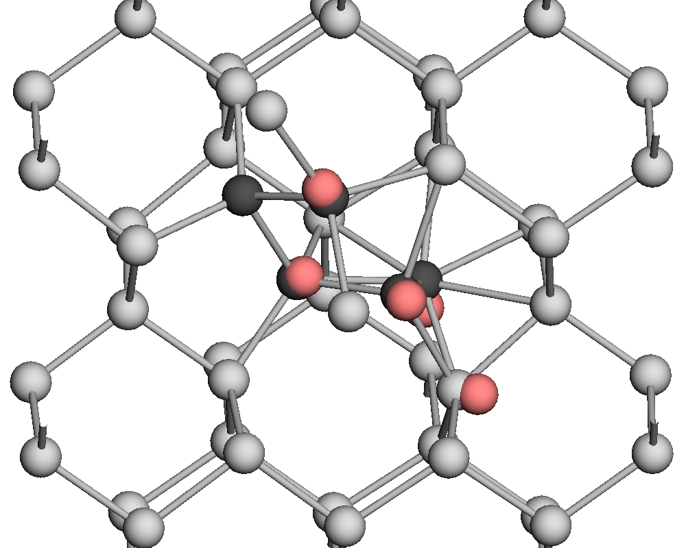
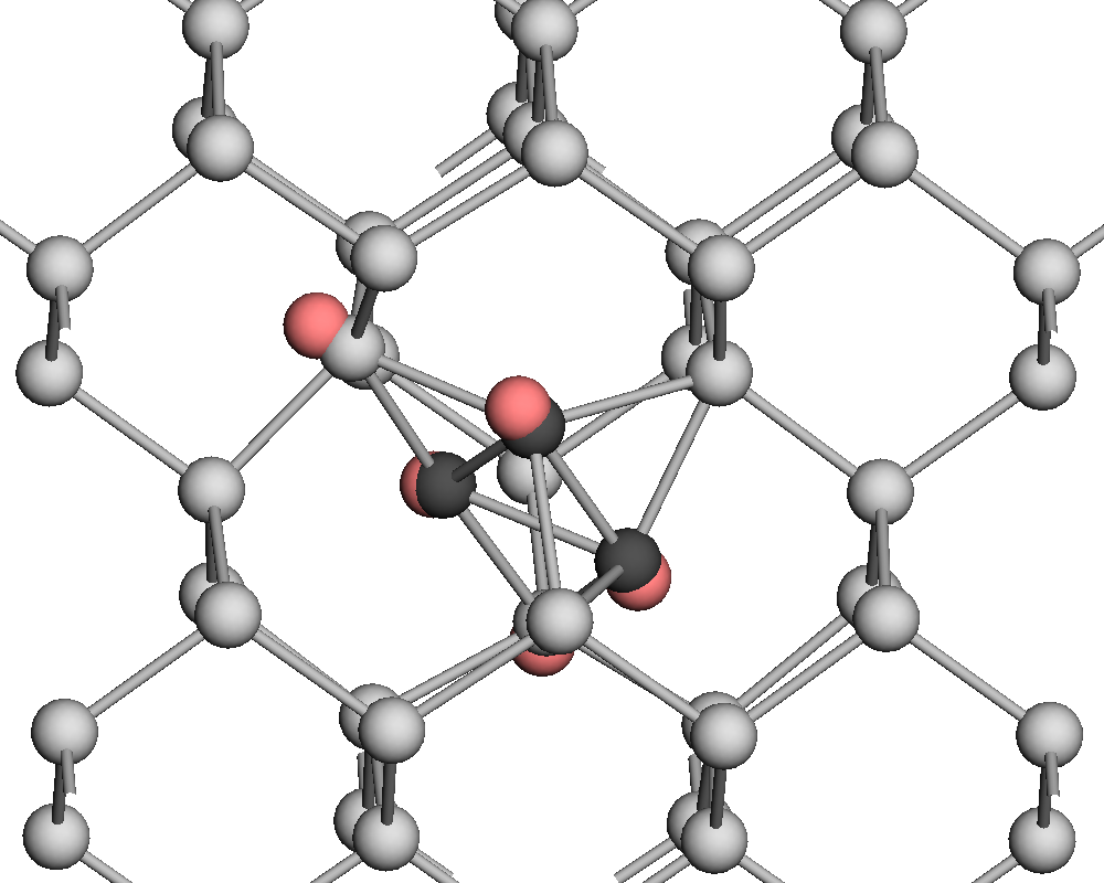
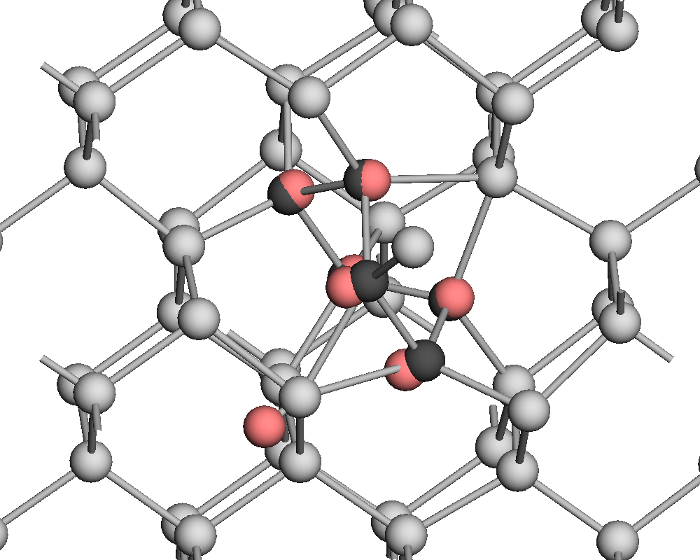
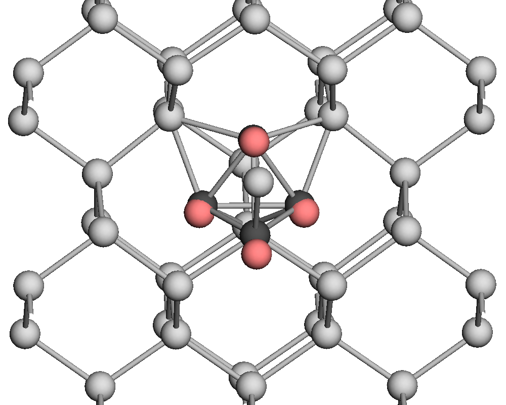
	XX3	TT	EXT	W	XEX	XT

Figure 27: Visualization of the atomic configurations of the relaxed di-interstitial structures with GAP (top row) and Stillinger-Weber (bottom row). Dark grey spheres show reference DFT-relaxed positions of defect atoms (those that are significantly different from perfect lattice position or topology), light grey spheres show reference DFT-relaxed positions of other atoms, and colored spheres show interatomic-potential-relaxed positions of defect atoms that are more than 0.1 Å from the corresponding DFT atom position.

V Conclusion

The benefit of the non-parametric approach for creating interatomic potentials, as presented here, is first and foremost its accuracy in matching the target potential energy surface. This enhanced accuracy is not just a quantitative improvement, but actually leads to a qualitatively better potential: the GAP model for silicon presented here provides a uniformly high accuracy across a wide range of properties and systems including bulk structures, point, and plane defects tested, while maintaining useful properties of conventional interatomic potentials: locality and linear scaling computational cost. This achievement requires an accurate description of the energetics of a wide range of configurations, including both fully bonded systems as well as bond breaking. The ability of the Si GAP to accurately describe both the energy and forces during the bond breaking process, including surface decohesion, unstable stacking fault minimum energy paths, and point defect migration barriers, is an especially important point which has been challenging for interatomic potentials to achieve due to their limited variational freedom and short range. Such a comprehensive description of silicon has never before been achieved, despite many efforts, with analytical potentials. The probabilistic nature of the Gaussian process technique allows for uncertainty quantification (and similar measures are possible to obtain using other non-parametric fitting techniques), and this is useful in assessing when configurations are encountered that are too far from the training set and are likely to have large errors. Initial efforts here strongly suggest that accuracy can be further improved for specific properties by adding relevant configurations to the database without compromising the accuracy for other properties.

There are of course limitations of the specific potential presented here. The major ones are that (i) we focused on only ambient pressure here, and a comprehensive silicon potential would be expected to reproduce the large variety of high pressure phases at finite temperatures; (ii) we limited ourselves to considering an elemental material. While it is true that increasing the number of different elements increases the dimensionality and therefore the complexity of the configuration space, several recent works found that including different atomic species do not qualitatively change the difficulty of the problem. De et al. (2016); Artrith et al. (2017) Another consequence of using the elemental silicon condensed phase example is that no long range interactions beyond 5 Å (such as Coulomb or van der Waals) are needed. Properly including long range interaction and integrating it with a high dimensional fit of the short range interactions is still an outstanding problem. Using a multi-scale description to capture these is an alternative approachHirn et al. (2017). Another deficiency of the present potential is that the training database was assembled “by hand”, using an ad hoc iterative process. It would be desirable to establish protocols that allow the essentially automated construction of databases suitable for predicting and studying specified macroscopic phenomena. There is every hope that the built-in uncertainty quantification can be used in the future to build much better databases and design algorithms that automatically select novel configurations encountered during a simulation for inclusion or even to generate new atomic configurations that are optimised to improve the database.

Finally, we are not making any claims about the optimality of the SOAP kernel and the corresponding basis functions. In particular, our implementation has a computational cost of around 100 ms/atom, and it is certainly possible that there are basis functions that are cheaper to calculate and better suited to the problem, so that fewer of them might be enough to achieve the same accuracy.Thompson et al. (2015); Shapeev (2016)

We believe that this potential, perhaps extended by the addition of particular geometries of interest or by a re-evaluation of the reference database with more accurate methods, will enable a new and more quantitative approach to simulations of structural properties of silicon.

We are well aware that the merits of the silicon potential presented here will not satisfy all possible audiences: while it is undeniable that the potential is far more accurate and transferable than any before it, its remaining shortcomings are not completely trivial, and only further work will conclusively show that they are easily overcome. Nevertheless, we hope that the present success in building a generally applicable potential will allow this to serve as a template for building such models for other materials, enabling scientifically and technologically relevant simulations that have thus far been limited by the tradeoffs between accuracy and computational cost.

The potential is available for anyone to use, and is provided in the form of an XML file for the QUIP code QUI as supplementary material. In addition to usage directly with QUIP, it can be used with the LAMMPSlam software with the “pair_style quip” command, as well as from ASELarsen et al. (2017) through QUIP’s quippy Python module. The datafile includes a copy of the training database structures and associated DFT data. The potential used throughout this paper has the unique label GAP_2017_6_17_60_4_3_56_165.