Stochastic Differential Equations Driven by Deterministic Chaotic Maps: Analytic Solutions of the Perron-Frobenius Equation

Griffin Williams and Christian Beck School of Mathematical Sciences, Queen Mary University of London, Mile End Road, London E1 4NS, UK
Abstract

We consider discrete-time dynamical systems with a linear relaxation dynamics that are driven by deterministic chaotic forces. By perturbative expansion in a small time scale parameter, we derive from the Perron-Frobenius equation the corrections to ordinary Fokker-Planck equations in leading order of the time scale separation parameter. We present analytic solutions to the equations for the example of driving forces generated by N𝑁N-th order Chebychev maps. The leading order corrections are universal for Nβ‰₯4𝑁4N\geq 4 but different for N=2𝑁2N=2 and N=3𝑁3N=3. We also study diffusively coupled Chebychev maps as driving forces, where strong correlations may prevent convergence to Gaussian limit behavior.

I Introduction

A fundamental problem lying at the roots of the foundations of statistical mechanics is the question of how Brownian motion and Langevin processes can arise from deterministic dynamical systems with strong mixing properties. This problem has been studied by many authors Bill -new5 . Due to the nature of the mixing property it is clear that a large phase-space dimension is not necessary to obtain β€˜random behavior’ of Brownian motion or Ornstein-Uhlenbeck type Bill , rather it is sufficient to consider low-dimensional mixing deterministic maps (with random initial conditions) and perform a suitable scaling limit, meaning looking at the ensemble of trajectories in a suitable rescaled way Roep -Beck5 . This is mathematically described by a time scale parameter Ο„πœ\tau which approaches 0. This parameter describes the ratio of the fast time scale underlying the deterministic chaotic driving force and the slow time scale corresponding to the relaxation time of the system.

In the simplest case, namely the case of a linear Langevin equation driven by chaotic β€˜noise’, the relevant class of dynamical systems where these concepts can be illustrated nicely, and mathematically treated rigorously, is given by maps of Kaplan-Yorke type Kaplan , sometimes also called maps of linear Langevin type Beck6 or skew products melbourne . They can be regarded as the deterministic chaotic analogue of a linear Langevin equation Kampen where the Gaussian white noise is replaced by a chaotic dynamics. In general, maps of linear Langevin type generate complicated (non-Gaussian, non-Markovian) stochastic processes, which, however, reduce to ordinary Gaussian behavior of Ornstein-Uhlenbeck type in the scaling limit Ο„β†’0β†’πœ0\tau\to 0 mentioned above, provided the driving map has sufficiently strong mixing behavior.

Of course, for small but finite Ο„πœ\tau there are corrections to the Gaussian limit behavior due to the underlying deterministic dynamics, which always has nontrivial correlations on a small scale, as it is deterministic on a small scale. In this paper we deal with the general question of what these corrections to Gaussian Langevin behavior are for general mixing driving forces, for small but finite Ο„πœ\tau. The driving dynamics is assumed to be generated by a map T𝑇T that has the so-called Ο†πœ‘\varphi-mixing property, a property that is sufficient to guarantee convergence to a Brownian motion process when the iterates are summed up and properly rescaled. We start from the Perron-Frobenius equation and then derive, by a perturbative expansion in Ο„πœ\sqrt{\tau}, a set of equations that is obeyed by the corrections to the Gaussian limit behavior. In 0-th order we get from this the Fokker-Planck equation, but our main goal is to solve the next-to-leading order equations. These turn out to be complicated functional equations. In this paper we show that we can explicitly solve the equations if the chaotic driving force is a Chebychev map of N𝑁N-th order, with N𝑁N arbitrary.

More complicated cases arise if the linear relaxation dynamics is driven by coupled maps kaneko ; buni . A dynamics driven by diffusively coupled Chebychev maps has applications in quantum field theory Beck7 -SM , providing a discrete dynamical version of the Parisi-Wu approach of stochastic quantization. The Perron-Frobenius equation cannot be solved analytically in this more complicated case, but still we will present some numerical results indicating how typical densities look like in this case, in particular how the kurtosis depends on the coupling strength of the coupled map lattice for small values of Ο„πœ\tau.

This paper is organized as follows:

In section 2 we perturbatively expand the Perron-Frobenius equation for the general type of dynamical systems considered in this paper. In section 3 we integrate out the chaotic forcing degrees of freedom and proceed to marginal densities (which correspond to the velocity of the kicked particle in the physical picture). In the following sections we then present the solution of the equations for general N𝑁N-th order Chebychev maps TNsubscript𝑇𝑁T_{N} as discrete-time driving forces. Each case N=2,3,4𝑁234N=2,3,4 requires a considerable amount of calculations. We start with the case N=2𝑁2N=2 in section 4, and then solve the functional equations for N=3𝑁3N=3 in section 5, and Nβ‰₯4𝑁4N\geq 4 in section 6. Technical details of the calculations can be found in the appendix.

In section 7 we will then finally compare our analytical predictions with numerical results. For the different N𝑁N we compare our analytically obtained results with numerically obtained histograms of iterates for different values of the time scale parameter Ο„πœ\tau. Excellent agreement between analytical and numerical results is obtained. In this section we will also present numerical results for cases that are not analytically tractable, such as the coupled Chebychev maps as driving forces as mentioned above. Our concluding remarks are given in section 8.

II Perturbative Expansion of the Perron-Frobenius Equation in the time scale parameter Ο„πœ\sqrt{\tau}

We start from a dynamical system of linear Langevin type Roep ; Beck1 ; Shim1 ; Beck5 ; new2 ; new4 ; new5 ; Yalcin ; Schlogl ; HC1 ; HC2

f:xn+1=T​(xn)yn+1=λ​yn+Ο„1/2​xn:𝑓subscriptπ‘₯𝑛1𝑇subscriptπ‘₯𝑛missing-subexpressionsubscript𝑦𝑛1πœ†subscript𝑦𝑛superscript𝜏12subscriptπ‘₯𝑛missing-subexpressionf:\begin{array}[]{ll}x_{n+1}=T\left(x_{n}\right)\\ y_{n+1}=\lambda y_{n}+\tau^{1/2}x_{n}\end{array} (1)

Here λ∈(0,1)πœ†01\lambda\in(0,1) and Ο„>0𝜏0\tau>0 are parameters, and T:Xβ†’X:𝑇→𝑋𝑋T:X\rightarrow X is some mapping that has strong mixing properties such that convergence to a Gaussian stochastic process Y​(t)π‘Œπ‘‘Y(t) is guaranteed in the limit Ο„β†’0,Ξ»β†’1,t=n​τformulae-sequenceβ†’πœ0formulae-sequenceβ†’πœ†1π‘‘π‘›πœ\tau\rightarrow 0,\ \lambda\rightarrow 1,\ t=n\tau finite. For example, the so-called Ο†πœ‘\varphi-mixing property is sufficient. We recall here that a stationary sequence {ΞΎn}subscriptπœ‰π‘›\{\xi_{n}\} of random variables is said to be Ο†πœ‘\varphi-mixing if the function φ​(n)πœ‘π‘›\varphi(n), defined by

Ο†(n)=supkβ©Ύ0supAβˆˆβ„¬kBβˆˆβ„¬k|m(Tβˆ’nA|B)βˆ’m(A)|(nβ‰₯0)\varphi(n)=\operatorname*{sup}_{k\geqslant 0}\ \operatorname*{\operatorname*{sup}_{A\in\mathscr{B}_{k}}}_{B\in\mathscr{B}^{k}}\ |m(T^{-n}A|B)-m(A)|\ \ (n\geq 0)

has the property φ​(n)β†’0​(nβ†’βˆž)β†’πœ‘π‘›0→𝑛\varphi(n)\rightarrow 0\ (n\rightarrow\infty). Here mπ‘šm denotes a suitable (natural) invariant measure of T𝑇T. Let ℬnsuperscriptℬ𝑛\mathscr{B}^{n} denote the ΟƒπœŽ\sigma-algebra generated by the random variables ΞΎ0,…,ΞΎnβˆ’1subscriptπœ‰0…subscriptπœ‰π‘›1\xi_{0},\dots,\xi_{n-1}, and ℬnsubscriptℬ𝑛\mathscr{B}_{n} denote the ΟƒπœŽ\sigma-algebra generated by ΞΎn,ΞΎn+1​…subscriptπœ‰π‘›subscriptπœ‰π‘›1…\xi_{n},\xi_{n+1}\dots. A map T𝑇T is said to be Ο†πœ‘\varphi-mixing if it admits a generating partition ΞΎπœ‰\xi such that the sequence ΞΎn=ξ∘Tnsubscriptπœ‰π‘›πœ‰superscript𝑇𝑛\xi_{n}=\xi\circ T^{n} is Ο†πœ‘\varphi-mixing Bill ; Roep . As a simple example, any map conjugated to a Bernoulli shift is Ο†πœ‘\varphi-mixing (with a vanishing Ο†πœ‘\varphi-function).

The map f𝑓f is a skew product extension of T𝑇T. Physically it is obtained by integration from the following deterministic chaotic analogue of a Langevin equation, which formally describes the velocity Yπ‘ŒY of a damped particle under deterministic chaotic kicks xnsubscriptπ‘₯𝑛x_{n}:

YΛ™=βˆ’Ξ³β€‹Y+Ο„1/2β€‹βˆ‘n=1∞xnβˆ’1​δ​(tβˆ’n​τ)Λ™π‘Œπ›Ύπ‘Œsuperscript𝜏12superscriptsubscript𝑛1subscriptπ‘₯𝑛1π›Ώπ‘‘π‘›πœ\dot{Y}=-\gamma Y+\tau^{1/2}\sum_{n=1}^{\infty}x_{n-1}\delta(t-n\tau) (2)
xn+1=T​(xn)subscriptπ‘₯𝑛1𝑇subscriptπ‘₯𝑛x_{n+1}=T(x_{n}) (3)

The map T𝑇T determines the time evolution of the kicks. Y​(t)π‘Œπ‘‘Y(t) can be regarded as the velocity of a kicked damped particle. Equation (1)1(1) describes the stroboscopic time evolution of yn:=Y​(n​τ+0)assignsubscriptπ‘¦π‘›π‘Œπ‘›πœ0y_{n}:=Y(n\tau+0). The damping constant Ξ³>0𝛾0\gamma>0 and the time difference Ο„πœ\tau between kicks are related to the parameter Ξ»πœ†\lambda by Ξ»=eβˆ’Ξ³β€‹Ο„πœ†superscriptπ‘’π›Ύπœ\lambda=e^{-\gamma\tau}. For concreteness we will deal with one-dimensional driving forces, although a similar analysis can be performed for higher-dimensional cases. The inverse map is given by

fβˆ’1:xn=Tβˆ’1​(xn+1)yn=Ξ»βˆ’1​(yn+1βˆ’Ο„1/2​Tβˆ’1​(xn+1)):superscript𝑓1subscriptπ‘₯𝑛superscript𝑇1subscriptπ‘₯𝑛1missing-subexpressionsubscript𝑦𝑛superscriptπœ†1subscript𝑦𝑛1superscript𝜏12superscript𝑇1subscriptπ‘₯𝑛1missing-subexpressionf^{-1}:\begin{array}[]{ll}x_{n}=T^{-1}(x_{n+1})\\ y_{n}=\lambda^{-1}(y_{n+1}-\tau^{1/2}T^{-1}(x_{n+1}))\end{array} (4)

In general, there are several preimages Tβˆ’1superscript𝑇1T^{-1}. The absolute value of the Jacobi determinant of f𝑓f is

|d​e​t​D​f|=λ​|T′​(x)|π‘‘π‘’π‘‘π·π‘“πœ†superscript𝑇′π‘₯|detDf|=\lambda|T^{\prime}(x)| (5)

The Perron-Frobenius equation

ρn+1​(xβ€²,yβ€²)=βˆ‘(x,y)∈fβˆ’1​(xβ€²,yβ€²)ρn​(x,y)λ​|T′​(x)|subscriptπœŒπ‘›1superscriptπ‘₯β€²superscript𝑦′subscriptπ‘₯𝑦superscript𝑓1superscriptπ‘₯β€²superscript𝑦′subscriptπœŒπ‘›π‘₯π‘¦πœ†superscript𝑇′π‘₯\rho_{n+1}(x^{\prime},y^{\prime})=\sum_{(x,y)\in f^{-1}(x^{\prime},y^{\prime})}\frac{\rho_{n}(x,y)}{\lambda|T^{\prime}(x)|} (6)

governs the time evolution of probability densities ρn​(x,y)subscriptπœŒπ‘›π‘₯𝑦\rho_{n}(x,y); it can be written as a sum over the preimages of T𝑇T:

λ​ρn+1​(xβ€²,y)=βˆ‘x∈Tβˆ’1​(xβ€²)1|T′​(x)|​ρn​(x,Ξ»βˆ’1​(yβˆ’Ο„1/2​x))πœ†subscriptπœŒπ‘›1superscriptπ‘₯′𝑦subscriptπ‘₯superscript𝑇1superscriptπ‘₯β€²1superscript𝑇′π‘₯subscriptπœŒπ‘›π‘₯superscriptπœ†1𝑦superscript𝜏12π‘₯\lambda\rho_{n+1}(x^{\prime},y)=\sum_{x\in T^{-1}(x^{\prime})}\frac{1}{|T^{\prime}(x)|}\rho_{n}(x,\lambda^{-1}(y-\tau^{1/2}x)) (7)

Equation (7)7(7), with Ξ»=eβˆ’Ξ³β€‹Ο„πœ†superscriptπ‘’π›Ύπœ\lambda=e^{-\gamma\tau}, is the starting point of our consideration. We will expand it with respect to the parameter Ο„1/2superscript𝜏12\tau^{1/2}, which is supposed to be small. Our main assumption is that such an expansion does make sense for suitable classes of maps T𝑇T and leads to a convergent series. We cannot prove this in general, but we will consider concrete examples of strongly mixing maps (N𝑁N-th order Chebychev maps) in this paper where indeed we show that the equations can be solved term by term in Ο„1/2superscript𝜏12\tau^{1/2}, leading to a series expansion that correctly describes the scaling behavior of the invariant density for small values of Ο„πœ\tau. In our perturbative analysis we will include all terms up to fourth order in Ο„1/2superscript𝜏12\tau^{1/2}. To simplify the notation, we will not explicitly write down any term of O​(Ο„5/2)𝑂superscript𝜏52O(\tau^{5/2}) or higher, but suppress it in all equations. Our numerics indeed indicates that higher order terms are negligible if Ο„πœ\tau is small enough (details of the numerics in Section VII). Without restriction of generality we set Ξ³=1𝛾1\gamma=1, obtaining up to fourth order in Ο„1/2superscript𝜏12\tau^{1/2}

Ξ»=eβˆ’Ο„=1βˆ’Ο„+12​τ2πœ†superscriptπ‘’πœ1𝜏12superscript𝜏2\lambda=e^{-\tau}=1-\tau+\frac{1}{2}\tau^{2} (8)

Since

Ξ»βˆ’1​(yβˆ’Ο„1/2​x)=(1+Ο„+12​τ2)​(yβˆ’Ο„1/2​x)superscriptπœ†1𝑦superscript𝜏12π‘₯1𝜏12superscript𝜏2𝑦superscript𝜏12π‘₯\lambda^{-1}(y-\tau^{1/2}x)=(1+\tau+\frac{1}{2}\tau^{2})(y-\tau^{1/2}x) (9)
=yβˆ’Ο„1/2​x+τ​yβˆ’Ο„3/2​x+12​τ2​yabsent𝑦superscript𝜏12π‘₯πœπ‘¦superscript𝜏32π‘₯12superscript𝜏2𝑦=y-\tau^{1/2}x+\tau y-\tau^{3/2}x+\frac{1}{2}\tau^{2}y (10)

we obtain by Taylor expansion

ρn​(x,Ξ»βˆ’1​(yβˆ’Ο„1/2​x))subscriptπœŒπ‘›π‘₯superscriptπœ†1𝑦superscript𝜏12π‘₯\displaystyle\rho_{n}(x,\lambda^{-1}(y-\tau^{1/2}x)) (11)
=ρn​(x,y)+(βˆ’Ο„1/2​x+τ​yβˆ’Ο„3/2​x+12​τ2​y)β€‹βˆ‚βˆ‚y​ρn​(x,y)absentsubscriptπœŒπ‘›π‘₯𝑦superscript𝜏12π‘₯πœπ‘¦superscript𝜏32π‘₯12superscript𝜏2𝑦𝑦subscriptπœŒπ‘›π‘₯𝑦\displaystyle={}\rho_{n}(x,y)+\left(-\tau^{1/2}x+\tau y-\tau^{3/2}x+\frac{1}{2}\tau^{2}y\right)\frac{\partial}{\partial y}\rho_{n}(x,y)
+12​(τ​x2+Ο„2​y2βˆ’2​τ3/2​x​y+2​τ2​x2)β€‹βˆ‚2βˆ‚y2​ρn​(x,y)12𝜏superscriptπ‘₯2superscript𝜏2superscript𝑦22superscript𝜏32π‘₯𝑦2superscript𝜏2superscriptπ‘₯2superscript2superscript𝑦2subscriptπœŒπ‘›π‘₯𝑦\displaystyle+\frac{1}{2}(\tau x^{2}+\tau^{2}y^{2}-2\tau^{3/2}xy+2\tau^{2}x^{2})\frac{\partial^{2}}{\partial y^{2}}\rho_{n}(x,y)
+16​(βˆ’Ο„3/2​x3+3​τ2​x2​y)β€‹βˆ‚3βˆ‚y3​ρn​(x,y)+124​τ2​x4β€‹βˆ‚4βˆ‚y4​ρn​(x,y)16superscript𝜏32superscriptπ‘₯33superscript𝜏2superscriptπ‘₯2𝑦superscript3superscript𝑦3subscriptπœŒπ‘›π‘₯𝑦124superscript𝜏2superscriptπ‘₯4superscript4superscript𝑦4subscriptπœŒπ‘›π‘₯𝑦\displaystyle+\frac{1}{6}(-\tau^{3/2}x^{3}+3\tau^{2}x^{2}y)\frac{\partial^{3}}{\partial y^{3}}\rho_{n}(x,y)+\frac{1}{24}\tau^{2}x^{4}\frac{\partial^{4}}{\partial y^{4}}\rho_{n}(x,y)
=ρn​(x,y)+Ο„1/2​[βˆ’xβ€‹βˆ‚βˆ‚y​ρn​(x,y)]absentsubscriptπœŒπ‘›π‘₯𝑦superscript𝜏12delimited-[]π‘₯𝑦subscriptπœŒπ‘›π‘₯𝑦\displaystyle=\rho_{n}(x,y)+\tau^{1/2}\left[-x\frac{\partial}{\partial y}\rho_{n}(x,y)\right]
+τ​[yβ€‹βˆ‚βˆ‚y​ρn​(x,y)+12​x2β€‹βˆ‚2βˆ‚y2​ρn​(x,y)]𝜏delimited-[]𝑦𝑦subscriptπœŒπ‘›π‘₯𝑦12superscriptπ‘₯2superscript2superscript𝑦2subscriptπœŒπ‘›π‘₯𝑦\displaystyle+\tau\left[y\frac{\partial}{\partial y}\rho_{n}(x,y)+\frac{1}{2}x^{2}\frac{\partial^{2}}{\partial y^{2}}\rho_{n}(x,y)\right]
+Ο„3/2​[βˆ’xβ€‹βˆ‚βˆ‚y​ρn​(x,y)βˆ’x​yβ€‹βˆ‚2βˆ‚y2​ρn​(x,y)βˆ’16​x3β€‹βˆ‚3βˆ‚y3​ρn​(x,y)]superscript𝜏32delimited-[]π‘₯𝑦subscriptπœŒπ‘›π‘₯𝑦π‘₯𝑦superscript2superscript𝑦2subscriptπœŒπ‘›π‘₯𝑦16superscriptπ‘₯3superscript3superscript𝑦3subscriptπœŒπ‘›π‘₯𝑦\displaystyle+\tau^{3/2}\left[-x\frac{\partial}{\partial y}\rho_{n}(x,y)-xy\frac{\partial^{2}}{\partial y^{2}}\rho_{n}(x,y)-\frac{1}{6}x^{3}\frac{\partial^{3}}{\partial y^{3}}\rho_{n}(x,y)\right]
+Ο„2[12yβˆ‚βˆ‚yρn(x,y)+12y2βˆ‚2βˆ‚y2ρn(x,y)+x2βˆ‚2βˆ‚y2ρn(x,y)\displaystyle+\tau^{2}\biggl{[}\frac{1}{2}y\frac{\partial}{\partial y}\rho_{n}(x,y)+\frac{1}{2}y^{2}\frac{\partial^{2}}{\partial y^{2}}\rho_{n}(x,y)+x^{2}\frac{\partial^{2}}{\partial y^{2}}\rho_{n}(x,y)
+12x2yβˆ‚3βˆ‚y3ρn(x,y)+124x4βˆ‚4βˆ‚y4ρn(x,y)]\displaystyle+\frac{1}{2}x^{2}y\frac{\partial^{3}}{\partial y^{3}}\rho_{n}(x,y)+\frac{1}{24}x^{4}\frac{\partial^{4}}{\partial y^{4}}\rho_{n}(x,y)\biggr{]}

Let us introduce a continuous-time suspension ρ​(x,y,t)𝜌π‘₯𝑦𝑑\rho(x,y,t) defined by

ρn​(x,y)=ρ​(x,y,t)(t=n​τ)subscriptπœŒπ‘›π‘₯π‘¦πœŒπ‘₯π‘¦π‘‘π‘‘π‘›πœ\rho_{n}(x,y)=\rho(x,y,t)\ \ \ \ (t=n\tau) (12)

By such a continuous-time suspension we mean a function ρ​(x,y,t)𝜌π‘₯𝑦𝑑\rho(x,y,t) depending on a continuous time variable t𝑑t such that at stroboscopic times t=nβ€‹Ο„π‘‘π‘›πœt=n\tau it coincides with ρn​(x,y)subscriptπœŒπ‘›π‘₯𝑦\rho_{n}(x,y). Since we keep Ο„πœ\tau small but finite, there are infinitely many such smooth functions ρ​(x,y,t)𝜌π‘₯𝑦𝑑\rho(x,y,t). At the present stage, we need not fix the function ρ​(x,y,t)𝜌π‘₯𝑦𝑑\rho(x,y,t) for time values t𝑑t other than discrete values nβ€‹Ο„π‘›πœn\tau. The following considerations are valid for any smooth suspension ρ​(x,y,t)𝜌π‘₯𝑦𝑑\rho(x,y,t) satisfying Eq. (12)12(12). A Taylor expansion yields

ρn+1​(x,y)=subscriptπœŒπ‘›1π‘₯𝑦absent\displaystyle\rho_{n+1}(x,y)={} ρ​(x,y,n​τ+Ο„)𝜌π‘₯π‘¦π‘›πœπœ\displaystyle\rho(x,y,n\tau+\tau)
=ρ​(x,y,n​τ)+Ο„β€‹βˆ‚βˆ‚t​ρ​(x,y,n​τ)+12​τ2β€‹βˆ‚2βˆ‚t2​ρ​(x,y,n​τ)absent𝜌π‘₯π‘¦π‘›πœπœπ‘‘πœŒπ‘₯π‘¦π‘›πœ12superscript𝜏2superscript2superscript𝑑2𝜌π‘₯π‘¦π‘›πœ\displaystyle=\rho(x,y,n\tau)+\tau\frac{\partial}{\partial t}\rho(x,y,n\tau)+\frac{1}{2}\tau^{2}\frac{\partial^{2}}{\partial t^{2}}\rho(x,y,n\tau)

Hence

λ​ρn+1​(xβ€²,y)πœ†subscriptπœŒπ‘›1superscriptπ‘₯′𝑦\displaystyle\lambda\rho_{n+1}(x^{\prime},y) (13)
=(1βˆ’Ο„+12​τ2)​[ρ​(xβ€²,y,t)+Ο„β€‹βˆ‚βˆ‚t​ρ​(xβ€²,y,t)+12​τ2β€‹βˆ‚2βˆ‚t2​ρ​(xβ€²,y,t)]absent1𝜏12superscript𝜏2delimited-[]𝜌superscriptπ‘₯β€²π‘¦π‘‘πœπ‘‘πœŒsuperscriptπ‘₯′𝑦𝑑12superscript𝜏2superscript2superscript𝑑2𝜌superscriptπ‘₯′𝑦𝑑\displaystyle={}\left(1-\tau+\frac{1}{2}\tau^{2}\right)\left[\rho(x^{\prime},y,t)+\tau\frac{\partial}{\partial t}\rho(x^{\prime},y,t)+\frac{1}{2}\tau^{2}\frac{\partial^{2}}{\partial t^{2}}\rho(x^{\prime},y,t)\right]
=ρ​(xβ€²,y,t)+τ​[βˆ’Οβ€‹(xβ€²,y,t)+βˆ‚βˆ‚t​ρ​(xβ€²,y,t)]absent𝜌superscriptπ‘₯β€²π‘¦π‘‘πœdelimited-[]𝜌superscriptπ‘₯β€²π‘¦π‘‘π‘‘πœŒsuperscriptπ‘₯′𝑦𝑑\displaystyle=\rho(x^{\prime},y,t)+\tau\left[-\rho(x^{\prime},y,t)+\frac{\partial}{\partial t}\rho(x^{\prime},y,t)\right]
+Ο„2​[12​ρ​(xβ€²,y,t)βˆ’βˆ‚βˆ‚t​ρ​(xβ€²,y,t)+12β€‹βˆ‚2βˆ‚t2​ρ​(xβ€²,y,t)](t=n​τ)superscript𝜏2delimited-[]12𝜌superscriptπ‘₯β€²π‘¦π‘‘π‘‘πœŒsuperscriptπ‘₯′𝑦𝑑12superscript2superscript𝑑2𝜌superscriptπ‘₯β€²π‘¦π‘‘π‘‘π‘›πœ\displaystyle+\tau^{2}\left[\frac{1}{2}\rho(x^{\prime},y,t)-\frac{\partial}{\partial t}\rho(x^{\prime},y,t)+\frac{1}{2}\frac{\partial^{2}}{\partial t^{2}}\rho(x^{\prime},y,t)\right]\ \ \ \ (t=n\tau)

The function ρ​(x,y,t)𝜌π‘₯𝑦𝑑\rho(x,y,t) still depends on Ξ»πœ†\lambda and thus on Ο„1/2superscript𝜏12\tau^{1/2}, since for stroboscopic times t=nβ€‹Ο„π‘‘π‘›πœt=n\tau it is the density ρ​(x,y)𝜌π‘₯𝑦\rho(x,y) of the map (1)1(1) which explicitly depends on Ξ»πœ†\lambda. In the spirit of van Kampen’s ΩΩ\Omega-expansion Kampen , we now make the following ansatz:

ρ​(x,y,t)=𝜌π‘₯𝑦𝑑absent\displaystyle\rho(x,y,t)={} φ​(x,y,t)+Ο„1/2​a​(x,y,t)+τ​b​(x,y,t)πœ‘π‘₯𝑦𝑑superscript𝜏12π‘Žπ‘₯π‘¦π‘‘πœπ‘π‘₯𝑦𝑑\displaystyle\varphi(x,y,t)+\tau^{1/2}a(x,y,t)+\tau b(x,y,t) (14)
+Ο„3/2​c​(x,y,t)+Ο„2​d​(x,y,t),superscript𝜏32𝑐π‘₯𝑦𝑑superscript𝜏2𝑑π‘₯𝑦𝑑\displaystyle+\tau^{3/2}c(x,y,t)+\tau^{2}d(x,y,t),

where the functions Ο†,a,b,c,πœ‘π‘Žπ‘π‘\varphi,a,b,c, and d𝑑d are assumed to be independent of Ο„πœ\tau. In our expansion all functions Ο†,a,b,c,dπœ‘π‘Žπ‘π‘π‘‘\varphi,a,b,c,d are assumed to be smooth such that they can be differentiated as often as required. For the concrete examples of maps T𝑇T studied in this paper, we will indeed find such smooth differentiable solutions to the equations in the later sections.

By putting the ansatz (14)14(14) into Eqs. (11)11(11) and (13)13(13) and comparing different powers of Ο„1/2superscript𝜏12\tau^{1/2}, one finally obtains the following five coupled functional equations for Ο†,a,b,c,πœ‘π‘Žπ‘π‘\varphi,a,b,c, and d𝑑d:

φ​(xβ€²,y,t)=βˆ‘x∈Tβˆ’1​(xβ€²)1|T′​(x)|​φ​(x,y,t)πœ‘superscriptπ‘₯′𝑦𝑑subscriptπ‘₯superscript𝑇1superscriptπ‘₯β€²1superscript𝑇′π‘₯πœ‘π‘₯𝑦𝑑\varphi(x^{\prime},y,t)=\sum_{x\in T^{-1}(x^{\prime})}\frac{1}{|T^{\prime}(x)|}\varphi(x,y,t) (15)
a​(xβ€²,y,t)=βˆ‘x∈Tβˆ’1​(xβ€²)1|T′​(x)|​[a​(x,y,t)βˆ’xβ€‹βˆ‚βˆ‚y​φ​(x,y,t)]π‘Žsuperscriptπ‘₯′𝑦𝑑subscriptπ‘₯superscript𝑇1superscriptπ‘₯β€²1superscript𝑇′π‘₯delimited-[]π‘Žπ‘₯𝑦𝑑π‘₯π‘¦πœ‘π‘₯𝑦𝑑a(x^{\prime},y,t)=\sum_{x\in T^{-1}(x^{\prime})}\frac{1}{|T^{\prime}(x)|}\biggl{[}a(x,y,t)-x\frac{\partial}{\partial y}\varphi(x,y,t)\biggr{]} (16)
b​(xβ€²,y,t)=𝑏superscriptπ‘₯′𝑦𝑑absent\displaystyle b(x^{\prime},y,t)={} βˆ‘x∈Tβˆ’1​(xβ€²)1|T′​(x)|[b(x,y,t)βˆ’xβˆ‚βˆ‚ya(x,y,t)\displaystyle\sum_{x\in T^{-1}(x^{\prime})}\frac{1}{|T^{\prime}(x)|}\biggl{[}b(x,y,t)-x\frac{\partial}{\partial y}a(x,y,t) (17)
+βˆ‚βˆ‚y(yΟ†(x,y,t))+12x2βˆ‚2βˆ‚y2Ο†(x,y,t)βˆ’βˆ‚βˆ‚tΟ†(x,y,t)]\displaystyle+\frac{\partial}{\partial y}(y\varphi(x,y,t))+\frac{1}{2}x^{2}\frac{\partial^{2}}{\partial y^{2}}\varphi(x,y,t)-\frac{\partial}{\partial t}\varphi(x,y,t)\biggr{]}
c​(xβ€²,y,t)=𝑐superscriptπ‘₯′𝑦𝑑absent\displaystyle c(x^{\prime},y,t)={} βˆ‘x∈Tβˆ’1​(xβ€²)1|T′​(x)|[c(x,y,t)βˆ’xβˆ‚βˆ‚yb(x,y,t)\displaystyle\sum_{x\in T^{-1}(x^{\prime})}\frac{1}{|T^{\prime}(x)|}\biggl{[}c(x,y,t)-x\frac{\partial}{\partial y}b(x,y,t) (18)
+βˆ‚βˆ‚y​(y​a​(x,y,t))+12​x2β€‹βˆ‚2βˆ‚y2​a​(x,y,t)βˆ’βˆ‚βˆ‚t​a​(x,y,t)π‘¦π‘¦π‘Žπ‘₯𝑦𝑑12superscriptπ‘₯2superscript2superscript𝑦2π‘Žπ‘₯π‘¦π‘‘π‘‘π‘Žπ‘₯𝑦𝑑\displaystyle+\frac{\partial}{\partial y}(ya(x,y,t))+\frac{1}{2}x^{2}\frac{\partial^{2}}{\partial y^{2}}a(x,y,t)-\frac{\partial}{\partial t}a(x,y,t)
βˆ’2​xβ€‹βˆ‚βˆ‚y​φ​(x,y,t)+xβ€‹βˆ‚βˆ‚yβ€‹βˆ‚βˆ‚t​φ​(x,y,t)βˆ’x​yβ€‹βˆ‚2βˆ‚y2​φ​(x,y,t)2π‘₯π‘¦πœ‘π‘₯𝑦𝑑π‘₯π‘¦π‘‘πœ‘π‘₯𝑦𝑑π‘₯𝑦superscript2superscript𝑦2πœ‘π‘₯𝑦𝑑\displaystyle-2x\frac{\partial}{\partial y}\varphi(x,y,t)+x\frac{\partial}{\partial y}\frac{\partial}{\partial t}\varphi(x,y,t)-xy\frac{\partial^{2}}{\partial y^{2}}\varphi(x,y,t)
βˆ’16x3βˆ‚3βˆ‚y3Ο†(x,y,t)]\displaystyle-\frac{1}{6}x^{3}\frac{\partial^{3}}{\partial y^{3}}\varphi(x,y,t)\biggr{]}
d​(xβ€²,y,t)=𝑑superscriptπ‘₯′𝑦𝑑absent\displaystyle d(x^{\prime},y,t)={} βˆ‘x∈Tβˆ’1​(xβ€²)1|T′​(x)|{d(x,y,t)βˆ’xβˆ‚βˆ‚yc(x,y,t)+βˆ‚βˆ‚y(yb(x,y,t))\displaystyle\sum_{x\in T^{-1}(x^{\prime})}\frac{1}{|T^{\prime}(x)|}\bigg{\{}d(x,y,t)-x\frac{\partial}{\partial y}c(x,y,t)+\frac{\partial}{\partial y}(yb(x,y,t)) (19)
+12​x2β€‹βˆ‚2βˆ‚y2​b​(x,y,t)βˆ’βˆ‚βˆ‚t​b​(x,y,t)12superscriptπ‘₯2superscript2superscript𝑦2𝑏π‘₯𝑦𝑑𝑑𝑏π‘₯𝑦𝑑\displaystyle+\frac{1}{2}x^{2}\frac{\partial^{2}}{\partial y^{2}}b(x,y,t)-\frac{\partial}{\partial t}b(x,y,t)
+x​[βˆ’2+βˆ‚βˆ‚tβˆ’yβ€‹βˆ‚βˆ‚yβˆ’16​x2β€‹βˆ‚2βˆ‚y2]β€‹βˆ‚βˆ‚y​a​(x,y,t)π‘₯delimited-[]2𝑑𝑦𝑦16superscriptπ‘₯2superscript2superscript𝑦2π‘¦π‘Žπ‘₯𝑦𝑑\displaystyle+x\left[-2+\frac{\partial}{\partial t}-y\frac{\partial}{\partial y}-\frac{1}{6}x^{2}\frac{\partial^{2}}{\partial y^{2}}\right]\frac{\partial}{\partial y}a(x,y,t)
+βˆ‚βˆ‚y​(y​φ​(x,y,t))+12​x2β€‹βˆ‚2βˆ‚y2​φ​(x,y,t)βˆ’βˆ‚βˆ‚t​φ​(x,y,t)π‘¦π‘¦πœ‘π‘₯𝑦𝑑12superscriptπ‘₯2superscript2superscript𝑦2πœ‘π‘₯π‘¦π‘‘π‘‘πœ‘π‘₯𝑦𝑑\displaystyle+\frac{\partial}{\partial y}(y\varphi(x,y,t))+\frac{1}{2}x^{2}\frac{\partial^{2}}{\partial y^{2}}\varphi(x,y,t)-\frac{\partial}{\partial t}\varphi(x,y,t)
βˆ’βˆ‚βˆ‚t​[βˆ‚βˆ‚y​(y​φ​(x,y,t))+12​x2β€‹βˆ‚2βˆ‚y2​φ​(x,y,t)βˆ’βˆ‚βˆ‚t​φ​(x,y,t)]𝑑delimited-[]π‘¦π‘¦πœ‘π‘₯𝑦𝑑12superscriptπ‘₯2superscript2superscript𝑦2πœ‘π‘₯π‘¦π‘‘π‘‘πœ‘π‘₯𝑦𝑑\displaystyle-\frac{\partial}{\partial t}\left[\frac{\partial}{\partial y}(y\varphi(x,y,t))+\frac{1}{2}x^{2}\frac{\partial^{2}}{\partial y^{2}}\varphi(x,y,t)-\frac{\partial}{\partial t}\varphi(x,y,t)\right]
+12​yβ€‹βˆ‚βˆ‚y​φ​(x,y,t)+12​y2β€‹βˆ‚2βˆ‚y2​φ​(x,y,t)12π‘¦π‘¦πœ‘π‘₯𝑦𝑑12superscript𝑦2superscript2superscript𝑦2πœ‘π‘₯𝑦𝑑\displaystyle+\frac{1}{2}y\frac{\partial}{\partial y}\varphi(x,y,t)+\frac{1}{2}y^{2}\frac{\partial^{2}}{\partial y^{2}}\varphi(x,y,t)
+x2​[1+12​yβ€‹βˆ‚βˆ‚y+124​x2β€‹βˆ‚2βˆ‚y2]β€‹βˆ‚2βˆ‚y2​φ​(x,y,t)superscriptπ‘₯2delimited-[]112𝑦𝑦124superscriptπ‘₯2superscript2superscript𝑦2superscript2superscript𝑦2πœ‘π‘₯𝑦𝑑\displaystyle+x^{2}\left[1+\frac{1}{2}y\frac{\partial}{\partial y}+\frac{1}{24}x^{2}\frac{\partial^{2}}{\partial y^{2}}\right]\frac{\partial^{2}}{\partial y^{2}}\varphi(x,y,t)
βˆ’12Ο†(x,y,t)+βˆ‚βˆ‚tΟ†(x,y,t)βˆ’12βˆ‚2βˆ‚t2Ο†(x,y,t)}\displaystyle-\frac{1}{2}\varphi(x,y,t)+\frac{\partial}{\partial t}\varphi(x,y,t)-\frac{1}{2}\frac{\partial^{2}}{\partial t^{2}}\varphi(x,y,t)\bigg{\}}

Notice that the last term on the right-hand side of Eq. (17)17(17) is a Fokker-Planck operator with non-constant variance x2superscriptπ‘₯2x^{2}, similar in spirit as for the superstatistics approach super1 ; super2 . Note that in the superstatistics approach one studies spatio-temporal systems with inhomogeneous temperature distributions T𝑇T, meaning the diffusion constant D∼k​Tsimilar-toπ·π‘˜π‘‡D\sim kT is varying in space and/or time. The term 12​x212superscriptπ‘₯2\frac{1}{2}x^{2} in front of the term βˆ‚2βˆ‚y2​φ​(x,y,t)superscript2superscript𝑦2πœ‘π‘₯𝑦𝑑\frac{\partial^{2}}{\partial y^{2}}\varphi(x,y,t) in Eq. (17) can formally be interpreted as a varying diffusion constant of a local Fokker-Planck equation for the function φ​(x,y,t)πœ‘π‘₯𝑦𝑑\varphi(x,y,t), and later we will integrate over all possible xπ‘₯x, similar in spirit to the superstatistics approach, where an ensemble of diffusion constants is considered super1 ; super2 ; nature-e . Equation (17)17(17) is a kind of combination of a Perron-Frobenius equation for the map T𝑇T with a Fokker-Planck equation, where the variance is not constant, but given by x2superscriptπ‘₯2x^{2}.

III Equations for marginal velocity distributions

In physical measurements of a particle that moves under deterministic chaotic kicks xnsubscriptπ‘₯𝑛x_{n}, one is interested in the probability distribution of the velocity ynsubscript𝑦𝑛y_{n} of the particle, and not in the joint probability distribution of kick strength xnsubscriptπ‘₯𝑛x_{n} and velocity ynsubscript𝑦𝑛y_{n}. Therefore, from a physical point of view it makes sense to proceed to the marginal distribution

p​(y,t)=βˆ«π‘‘x​ρ​(x,y,t)𝑝𝑦𝑑differential-dπ‘₯𝜌π‘₯𝑦𝑑p(y,t)=\int dx\ \rho(x,y,t) (20)

of the y𝑦y variable, obtained by integration over all possible xπ‘₯x values. In the physical picture, p​(y,t)𝑝𝑦𝑑p(y,t) describes the velocity distribution of the particle, which is kicked by deterministic chaotic iterates xnsubscriptπ‘₯𝑛x_{n}, whereas ρ​(x,y,t)𝜌π‘₯𝑦𝑑\rho(x,y,t) has no direct physical interpretation. For tβ†’βˆžβ†’π‘‘t\to\infty, the stationary distribution is obtained, denoted by p​(y)𝑝𝑦p(y). The integration over xπ‘₯x indeed yields a simplification in our problem, transforming the coupled functional equations of the previous section into coupled differential equations.

Let us use the notation

p0​(y,t)=βˆ«π‘‘x​φ​(x,y,t)subscript𝑝0𝑦𝑑differential-dπ‘₯πœ‘π‘₯𝑦𝑑p_{0}(y,t)=\int dx\ \varphi(x,y,t) (21)
α​(y,t)=βˆ«π‘‘x​a​(x,y,t)𝛼𝑦𝑑differential-dπ‘₯π‘Žπ‘₯𝑦𝑑\alpha(y,t)=\int dx\ a(x,y,t) (22)
β​(y,t)=βˆ«π‘‘x​b​(x,y,t)𝛽𝑦𝑑differential-dπ‘₯𝑏π‘₯𝑦𝑑\beta(y,t)=\int dx\ b(x,y,t) (23)
γ​(y,t)=βˆ«π‘‘x​c​(x,y,t)𝛾𝑦𝑑differential-dπ‘₯𝑐π‘₯𝑦𝑑\gamma(y,t)=\int dx\ c(x,y,t) (24)
δ​(y,t)=βˆ«π‘‘x​d​(x,y,t)𝛿𝑦𝑑differential-dπ‘₯𝑑π‘₯𝑦𝑑\delta(y,t)=\int dx\ d(x,y,t) (25)

From Eqs.(15)-(19) we obtain that the marginal functions satisfy

βˆ‚βˆ‚yβ€‹βˆ«π‘‘x​x​φ​(x,y,t)=0𝑦differential-dπ‘₯π‘₯πœ‘π‘₯𝑦𝑑0\frac{\partial}{\partial y}\int dx\ x\varphi(x,y,t)=0 (26)
βˆ‚βˆ‚yβ€‹βˆ«π‘‘x​x​a​(x,y,t)=βˆ‚βˆ‚y​(y​p0​(y,t))+12β€‹βˆ‚2βˆ‚y2β€‹βˆ«π‘‘x​x2​φ​(x,y,t)βˆ’βˆ‚βˆ‚t​p0​(y,t)𝑦differential-dπ‘₯π‘₯π‘Žπ‘₯𝑦𝑑𝑦𝑦subscript𝑝0𝑦𝑑12superscript2superscript𝑦2differential-dπ‘₯superscriptπ‘₯2πœ‘π‘₯𝑦𝑑𝑑subscript𝑝0𝑦𝑑\frac{\partial}{\partial y}\int dx\ xa(x,y,t)=\frac{\partial}{\partial y}(yp_{0}(y,t))+\frac{1}{2}\frac{\partial^{2}}{\partial y^{2}}\int dx\ x^{2}\varphi(x,y,t)-\frac{\partial}{\partial t}p_{0}(y,t) (27)
βˆ‚βˆ‚yβ€‹βˆ«π‘‘x​x​b​(x,y,t)=𝑦differential-dπ‘₯π‘₯𝑏π‘₯𝑦𝑑absent\displaystyle\frac{\partial}{\partial y}\int dx\ xb(x,y,t)={} βˆ‚βˆ‚y​(y​α​(y,t))+12β€‹βˆ‚2βˆ‚y2β€‹βˆ«π‘‘x​x2​a​(x,y,t)βˆ’βˆ‚βˆ‚t​α​(y,t)𝑦𝑦𝛼𝑦𝑑12superscript2superscript𝑦2differential-dπ‘₯superscriptπ‘₯2π‘Žπ‘₯𝑦𝑑𝑑𝛼𝑦𝑑\displaystyle\frac{\partial}{\partial y}(y\alpha(y,t))+\frac{1}{2}\frac{\partial^{2}}{\partial y^{2}}\int dx\ x^{2}a(x,y,t)-\frac{\partial}{\partial t}\alpha(y,t) (28)
+βˆ«π‘‘x​x​[βˆ’2+βˆ‚βˆ‚tβˆ’yβ€‹βˆ‚βˆ‚yβˆ’16​x2β€‹βˆ‚2βˆ‚y2]β€‹βˆ‚βˆ‚y​φ​(x,y,t)differential-dπ‘₯π‘₯delimited-[]2𝑑𝑦𝑦16superscriptπ‘₯2superscript2superscript𝑦2π‘¦πœ‘π‘₯𝑦𝑑\displaystyle+\int dx\ x\left[-2+\frac{\partial}{\partial t}-y\frac{\partial}{\partial y}-\frac{1}{6}x^{2}\frac{\partial^{2}}{\partial y^{2}}\right]\frac{\partial}{\partial y}\varphi(x,y,t)
βˆ‚βˆ‚yβ€‹βˆ«π‘‘x​x​c​(x,y,t)=𝑦differential-dπ‘₯π‘₯𝑐π‘₯𝑦𝑑absent\displaystyle\frac{\partial}{\partial y}\int dx\ xc(x,y,t)={} βˆ‚βˆ‚y​(y​β​(y,t))+12β€‹βˆ‚2βˆ‚y2β€‹βˆ«π‘‘x​x2​b​(x,y,t)βˆ’βˆ‚βˆ‚t​β​(y,t)𝑦𝑦𝛽𝑦𝑑12superscript2superscript𝑦2differential-dπ‘₯superscriptπ‘₯2𝑏π‘₯𝑦𝑑𝑑𝛽𝑦𝑑\displaystyle\frac{\partial}{\partial y}(y\beta(y,t))+\frac{1}{2}\frac{\partial^{2}}{\partial y^{2}}\int dx\ x^{2}b(x,y,t)-\frac{\partial}{\partial t}\beta(y,t) (29)
βˆ’βˆ«π‘‘x​x​[2βˆ’βˆ‚βˆ‚t+yβ€‹βˆ‚βˆ‚y+16​x2β€‹βˆ‚2βˆ‚y2]β€‹βˆ‚βˆ‚y​a​(x,y,t)differential-dπ‘₯π‘₯delimited-[]2𝑑𝑦𝑦16superscriptπ‘₯2superscript2superscript𝑦2π‘¦π‘Žπ‘₯𝑦𝑑\displaystyle-\int dx\ x\left[2-\frac{\partial}{\partial t}+y\frac{\partial}{\partial y}+\frac{1}{6}x^{2}\frac{\partial^{2}}{\partial y^{2}}\right]\frac{\partial}{\partial y}a(x,y,t)
+(1βˆ’βˆ‚βˆ‚t)[βˆ‚βˆ‚y(yp0(y,t))\displaystyle+\left(1-\frac{\partial}{\partial t}\right)\biggl{[}\frac{\partial}{\partial y}(yp_{0}(y,t))
+12βˆ‚2βˆ‚y2∫dxx2Ο†(x,y,t)βˆ’βˆ‚βˆ‚tp0(y,t)]\displaystyle+\frac{1}{2}\frac{\partial^{2}}{\partial y^{2}}\int dx\ x^{2}\varphi(x,y,t)-\frac{\partial}{\partial t}p_{0}(y,t)\biggr{]}
+[12​yβ€‹βˆ‚βˆ‚y+12​y2β€‹βˆ‚2βˆ‚y2βˆ’12+βˆ‚βˆ‚tβˆ’12β€‹βˆ‚2βˆ‚t2]​p0​(y,t)delimited-[]12𝑦𝑦12superscript𝑦2superscript2superscript𝑦212𝑑12superscript2superscript𝑑2subscript𝑝0𝑦𝑑\displaystyle+\left[\frac{1}{2}y\frac{\partial}{\partial y}+\frac{1}{2}y^{2}\frac{\partial^{2}}{\partial y^{2}}-\frac{1}{2}+\frac{\partial}{\partial t}-\frac{1}{2}\frac{\partial^{2}}{\partial t^{2}}\right]p_{0}(y,t)
+(βˆ‚2βˆ‚y2+12​yβ€‹βˆ‚3βˆ‚y3)β€‹βˆ«π‘‘x​x2​φ​(x,y,t)superscript2superscript𝑦212𝑦superscript3superscript𝑦3differential-dπ‘₯superscriptπ‘₯2πœ‘π‘₯𝑦𝑑\displaystyle+\left(\frac{\partial^{2}}{\partial y^{2}}+\frac{1}{2}y\frac{\partial^{3}}{\partial y^{3}}\right)\int dx\ x^{2}\varphi(x,y,t)
+124β€‹βˆ‚4βˆ‚y4β€‹βˆ«π‘‘x​x4​φ​(x,y,t)124superscript4superscript𝑦4differential-dπ‘₯superscriptπ‘₯4πœ‘π‘₯𝑦𝑑\displaystyle+\frac{1}{24}\frac{\partial^{4}}{\partial y^{4}}\int dx\ x^{4}\varphi(x,y,t)

Let us first deal with the zeroth-order term φ​(x,y,t)πœ‘π‘₯𝑦𝑑\varphi(x,y,t). Equation (15)15(15) is solved by any function φ​(x,y,t)πœ‘π‘₯𝑦𝑑\varphi(x,y,t) of the form

φ​(x,y,t)=h​(x)​p0​(y,t)πœ‘π‘₯π‘¦π‘‘β„Žπ‘₯subscript𝑝0𝑦𝑑\varphi(x,y,t)=h(x)p_{0}(y,t) (30)

where h​(x)β„Žπ‘₯h(x) is the natural invariant density of the T𝑇T-dynamics. To obtain a compact notation, we will use the notation βŸ¨β€¦βŸ©delimited-βŸ¨βŸ©β€¦\langle\dots\rangle for expectations with respect to h​(x)β„Žπ‘₯h(x). Equation (26)26(26) then implies

βˆ‚βˆ‚y​p0​(y,t)β€‹βˆ«π‘‘x​x​h​(x)=⟨xβŸ©β€‹βˆ‚βˆ‚y​p0​(y,t)=0𝑦subscript𝑝0𝑦𝑑differential-dπ‘₯π‘₯β„Žπ‘₯delimited-⟨⟩π‘₯𝑦subscript𝑝0𝑦𝑑0\frac{\partial}{\partial y}p_{0}(y,t)\int dx\ xh(x)=\langle x\rangle\frac{\partial}{\partial y}p_{0}(y,t)=0 (31)

In case that ρ0​(y,t)β‰ c​o​n​s​tysubscript𝜌0π‘¦π‘‘π‘π‘œπ‘›π‘ subscript𝑑𝑦\rho_{0}(y,t)\neq const_{y} this means ⟨x⟩=0delimited-⟨⟩π‘₯0\langle x\rangle=0, which shows that the ansatz (14)14(14) makes sense for maps with vanishing average only. Equation (27)27(27) becomes

βˆ‚βˆ‚y​(y​p0​(y,t))+12β€‹βŸ¨x2βŸ©β€‹βˆ‚2βˆ‚y2​p0​(y,t)βˆ’βˆ‚βˆ‚t​p0​(y,t)=βˆ‚βˆ‚yβ€‹βˆ«π‘‘x​x​a​(x,y,t)𝑦𝑦subscript𝑝0𝑦𝑑12delimited-⟨⟩superscriptπ‘₯2superscript2superscript𝑦2subscript𝑝0𝑦𝑑𝑑subscript𝑝0𝑦𝑑𝑦differential-dπ‘₯π‘₯π‘Žπ‘₯𝑦𝑑\frac{\partial}{\partial y}(yp_{0}(y,t))+\frac{1}{2}\langle x^{2}\rangle\frac{\partial^{2}}{\partial y^{2}}p_{0}(y,t)-\frac{\partial}{\partial t}p_{0}(y,t)=\frac{\partial}{\partial y}\int dx\ xa(x,y,t) (32)

This is a kind of inhomogeneous Fokker-Planck equation with a source term (βˆ‚/βˆ‚y)β€‹βˆ«π‘‘x​x​a​(x,y,t)𝑦differential-dπ‘₯π‘₯π‘Žπ‘₯𝑦𝑑(\partial/\partial y)\int dxxa(x,y,t). It reduces to a Fokker-Planck equation for the case that (βˆ‚/βˆ‚y)β€‹βˆ«π‘‘x​x​a​(x,y,t)=0𝑦differential-dπ‘₯π‘₯π‘Žπ‘₯𝑦𝑑0(\partial/\partial y)\int dxxa(x,y,t)=0. If (βˆ‚/βˆ‚y)β€‹βˆ«π‘‘x​x​a​(x,y,t)𝑦differential-dπ‘₯π‘₯π‘Žπ‘₯𝑦𝑑(\partial/\partial y)\int dxxa(x,y,t) is proportional to (βˆ‚2/βˆ‚y2)​ρ0​(y,t)superscript2superscript𝑦2subscript𝜌0𝑦𝑑(\partial^{2}/\partial y^{2})\rho_{0}(y,t), we also obtain a Fokker-Planck equation, but with a different diffusion constant. Hence, in order to determine ρ0​(y,t)subscript𝜌0𝑦𝑑\rho_{0}(y,t), we have to determine βˆ«π‘‘x​x​a​(x,y,t)differential-dπ‘₯π‘₯π‘Žπ‘₯𝑦𝑑\int dxxa(x,y,t) with the help of Eq. (16)16(16).

The equations simplify considerably for particular choices of mappings T𝑇T that have the property that both the mapping T𝑇T as well as its natural invariant density hβ„Žh are symmetric:

T​(x)=T​(βˆ’x)𝑇π‘₯𝑇π‘₯T(x)=T(-x) (33)
h​(x)=h​(βˆ’x)β„Žπ‘₯β„Žπ‘₯h(x)=h(-x) (34)

We call these types of maps double symmetric. Examples are maps conjugated to even Chebyshev polynomials. For double symmetric maps we have

βˆ‘x∈Tβˆ’1​(xβ€²)1|T′​(x)|​x​h​(x)β€‹βˆ‚βˆ‚y​p0​(y,t)=0subscriptπ‘₯superscript𝑇1superscriptπ‘₯β€²1superscript𝑇′π‘₯π‘₯β„Žπ‘₯𝑦subscript𝑝0𝑦𝑑0\sum_{x\in T^{-1}(x^{\prime})}\frac{1}{|T^{\prime}(x)|}xh(x)\frac{\partial}{\partial y}p_{0}(y,t)=0 (35)

since for each x,βˆ’xπ‘₯π‘₯x,-x is also a preimage. Hence Eq. (16)16(16) reduces to

a​(xβ€²,y,t)=βˆ‘x∈Tβˆ’1​(xβ€²)1|T′​(x)|​a​(x,y,t)π‘Žsuperscriptπ‘₯′𝑦𝑑subscriptπ‘₯superscript𝑇1superscriptπ‘₯β€²1superscript𝑇′π‘₯π‘Žπ‘₯𝑦𝑑a(x^{\prime},y,t)=\sum_{x\in T^{-1}(x^{\prime})}\frac{1}{|T^{\prime}(x)|}a(x,y,t) (36)

Notice that this is just the same equation as the one satisfied by Ο†πœ‘\varphi. It is solved by a function of the form

a​(x,y,t)=h​(x)​α​(y,t)π‘Žπ‘₯π‘¦π‘‘β„Žπ‘₯𝛼𝑦𝑑a(x,y,t)=h(x)\alpha(y,t) (37)

Moreover, we obtain

b​(xβ€²,y,t)=𝑏superscriptπ‘₯′𝑦𝑑absent\displaystyle b(x^{\prime},y,t)={} βˆ‘x∈Tβˆ’1​(xβ€²)1|T′​(x)|(b(x,y,t)+h(x)(βˆ‚βˆ‚y(yp0(y,t))\displaystyle\sum_{x\in T^{-1}(x^{\prime})}\frac{1}{|T^{\prime}(x)|}(b(x,y,t)+h(x)(\frac{\partial}{\partial y}(yp_{0}(y,t)) (38)
+12x2βˆ‚2βˆ‚y2p0(y,t)βˆ’βˆ‚βˆ‚tp0(y,t)))\displaystyle+\frac{1}{2}x^{2}\frac{\partial^{2}}{\partial y^{2}}p_{0}(y,t)-\frac{\partial}{\partial t}p_{0}(y,t)))
c​(xβ€²,y,t)=𝑐superscriptπ‘₯′𝑦𝑑absent\displaystyle c(x^{\prime},y,t)={} βˆ‘x∈Tβˆ’1​(xβ€²)1|T′​(x)|(c(x,y,t)βˆ’xβˆ‚βˆ‚yb(x,y,t)\displaystyle\sum_{x\in T^{-1}(x^{\prime})}\frac{1}{|T^{\prime}(x)|}(c(x,y,t)-x\frac{\partial}{\partial y}b(x,y,t) (39)
+h(x)[βˆ‚βˆ‚y(yΞ±(y,t))+12x2βˆ‚2βˆ‚y2Ξ±(y,t)βˆ’βˆ‚βˆ‚tΞ±(y,t)])\displaystyle+h(x)\left[\frac{\partial}{\partial y}(y\alpha(y,t))+\frac{1}{2}x^{2}\frac{\partial^{2}}{\partial y^{2}}\alpha(y,t)-\frac{\partial}{\partial t}\alpha(y,t)\right])
d​(xβ€²,y,t)=𝑑superscriptπ‘₯′𝑦𝑑absent\displaystyle d(x^{\prime},y,t)={} βˆ‘x∈Tβˆ’1​(xβ€²)1|T′​(x)|(d(x,y,t)βˆ’xβˆ‚βˆ‚yc(x,y,t)+βˆ‚βˆ‚y(yb(x,y,t))\displaystyle\sum_{x\in T^{-1}(x^{\prime})}\frac{1}{|T^{\prime}(x)|}(d(x,y,t)-x\frac{\partial}{\partial y}c(x,y,t)+\frac{\partial}{\partial y}(yb(x,y,t)) (40)
+12​x2β€‹βˆ‚2βˆ‚y2​b​(x,y,t)βˆ’βˆ‚βˆ‚t​b​(x,y,t)12superscriptπ‘₯2superscript2superscript𝑦2𝑏π‘₯𝑦𝑑𝑑𝑏π‘₯𝑦𝑑\displaystyle+\frac{1}{2}x^{2}\frac{\partial^{2}}{\partial y^{2}}b(x,y,t)-\frac{\partial}{\partial t}b(x,y,t)
+h(x)((1βˆ’βˆ‚βˆ‚t)(βˆ‚βˆ‚y(yp0(y,t))\displaystyle+h(x)(\left(1-\frac{\partial}{\partial t}\right)(\frac{\partial}{\partial y}(yp_{0}(y,t))
+12x2βˆ‚2βˆ‚y2p0(y,t)βˆ’βˆ‚βˆ‚tp0(y,t))\displaystyle+\frac{1}{2}x^{2}\frac{\partial^{2}}{\partial y^{2}}p_{0}(y,t)-\frac{\partial}{\partial t}p_{0}(y,t))
+12​yβ€‹βˆ‚βˆ‚y​p0​(y,t)+12​y2β€‹βˆ‚2βˆ‚y2​p0​(y,t)12𝑦𝑦subscript𝑝0𝑦𝑑12superscript𝑦2superscript2superscript𝑦2subscript𝑝0𝑦𝑑\displaystyle+\frac{1}{2}y\frac{\partial}{\partial y}p_{0}(y,t)+\frac{1}{2}y^{2}\frac{\partial^{2}}{\partial y^{2}}p_{0}(y,t)
+x2​(1+12​yβ€‹βˆ‚βˆ‚y+124​x2β€‹βˆ‚2βˆ‚y2)β€‹βˆ‚2βˆ‚y2​p0​(y,t)superscriptπ‘₯2112𝑦𝑦124superscriptπ‘₯2superscript2superscript𝑦2superscript2superscript𝑦2subscript𝑝0𝑦𝑑\displaystyle+x^{2}\left(1+\frac{1}{2}y\frac{\partial}{\partial y}+\frac{1}{24}x^{2}\frac{\partial^{2}}{\partial y^{2}}\right)\frac{\partial^{2}}{\partial y^{2}}p_{0}(y,t)
βˆ’12p0(y,t)+βˆ‚βˆ‚tp0(y,t)βˆ’12βˆ‚2βˆ‚t2p0(y,t)))\displaystyle-\frac{1}{2}p_{0}(y,t)+\frac{\partial}{\partial t}p_{0}(y,t)-\frac{1}{2}\frac{\partial^{2}}{\partial t^{2}}p_{0}(y,t)))

The integrated equations reduce to

0=βˆ‚βˆ‚y​(y​p0​(y,t))+12β€‹βŸ¨x2βŸ©β€‹βˆ‚2βˆ‚y2​p0​(y,t)βˆ’βˆ‚βˆ‚t​p0​(y,t)0𝑦𝑦subscript𝑝0𝑦𝑑12delimited-⟨⟩superscriptπ‘₯2superscript2superscript𝑦2subscript𝑝0𝑦𝑑𝑑subscript𝑝0𝑦𝑑0=\frac{\partial}{\partial y}(yp_{0}(y,t))+\frac{1}{2}\langle x^{2}\rangle\frac{\partial^{2}}{\partial y^{2}}p_{0}(y,t)-\frac{\partial}{\partial t}p_{0}(y,t) (41)
βˆ‚βˆ‚yβ€‹βˆ«π‘‘x​x​b​(x,y,t)=βˆ‚βˆ‚y​(y​α​(y,t))+12β€‹βŸ¨x2βŸ©β€‹βˆ‚2βˆ‚y2​α​(y,t)βˆ’βˆ‚βˆ‚t​α​(y,t)𝑦differential-dπ‘₯π‘₯𝑏π‘₯𝑦𝑑𝑦𝑦𝛼𝑦𝑑12delimited-⟨⟩superscriptπ‘₯2superscript2superscript𝑦2𝛼𝑦𝑑𝑑𝛼𝑦𝑑\frac{\partial}{\partial y}\int dx\ xb(x,y,t)=\frac{\partial}{\partial y}(y\alpha(y,t))+\frac{1}{2}\langle x^{2}\rangle\frac{\partial^{2}}{\partial y^{2}}\alpha(y,t)-\frac{\partial}{\partial t}\alpha(y,t) (42)
βˆ‚βˆ‚yβ€‹βˆ«π‘‘x​x​c​(x,y,t)=𝑦differential-dπ‘₯π‘₯𝑐π‘₯𝑦𝑑absent\displaystyle\frac{\partial}{\partial y}\int dx\ xc(x,y,t)={} βˆ‚βˆ‚y​(y​β​(y,t))+12β€‹βˆ‚2βˆ‚y2β€‹βˆ«π‘‘x​x2​b​(x,y,t)βˆ’βˆ‚βˆ‚t​β​(y,t)𝑦𝑦𝛽𝑦𝑑12superscript2superscript𝑦2differential-dπ‘₯superscriptπ‘₯2𝑏π‘₯𝑦𝑑𝑑𝛽𝑦𝑑\displaystyle\frac{\partial}{\partial y}(y\beta(y,t))+\frac{1}{2}\frac{\partial^{2}}{\partial y^{2}}\int dx\ x^{2}b(x,y,t)-\frac{\partial}{\partial t}\beta(y,t) (43)
+[12yβˆ‚βˆ‚y+12y2βˆ‚2βˆ‚y2+⟨x2βŸ©βˆ‚2βˆ‚y2+12⟨x2⟩yβˆ‚3βˆ‚y3\displaystyle+\biggl{[}\frac{1}{2}y\frac{\partial}{\partial y}+\frac{1}{2}y^{2}\frac{\partial^{2}}{\partial y^{2}}+\langle x^{2}\rangle\frac{\partial^{2}}{\partial y^{2}}+\frac{1}{2}\langle x^{2}\rangle y\frac{\partial^{3}}{\partial y^{3}}
+124⟨x4βŸ©βˆ‚4βˆ‚y4βˆ’12+βˆ‚βˆ‚tβˆ’12βˆ‚2βˆ‚t2]p0(y,t)\displaystyle+\frac{1}{24}\langle x^{4}\rangle\frac{\partial^{4}}{\partial y^{4}}-\frac{1}{2}+\frac{\partial}{\partial t}-\frac{1}{2}\frac{\partial^{2}}{\partial t^{2}}\biggr{]}p_{0}(y,t)

Notice that Eq. (41)41(41) is the Fokker-Planck equation. We obtain the result that for double-symmetric maps the diffusion constant is always given by ⟨x2⟩delimited-⟨⟩superscriptπ‘₯2\langle x^{2}\rangle. Equation (42)42(42) is the same type as Eq. (32)32(32); it is an inhomogeneous Fokker-Planck equation, but now - due to the condition of double symmetry - it is satisfied by α​(y,t)𝛼𝑦𝑑\alpha(y,t) rather that p0​(y,t)subscript𝑝0𝑦𝑑p_{0}(y,t).

Subtracting the zero given by Eq. (41)41(41) from the right-hand side of Eq. (38)38(38), we may also write Eq. (38)38(38) as

b​(xβ€²,y,t)=βˆ‘x∈Tβˆ’1​(xβ€²)1|T′​(x)|​[b​(x,y,t)+h​(x)​12​(x2βˆ’βŸ¨x2⟩)β€‹βˆ‚2βˆ‚y2​p0​(y,t)]𝑏superscriptπ‘₯′𝑦𝑑subscriptπ‘₯superscript𝑇1superscriptπ‘₯β€²1superscript𝑇′π‘₯delimited-[]𝑏π‘₯π‘¦π‘‘β„Žπ‘₯12superscriptπ‘₯2delimited-⟨⟩superscriptπ‘₯2superscript2superscript𝑦2subscript𝑝0𝑦𝑑b(x^{\prime},y,t)=\sum_{x\in T^{-1}(x^{\prime})}\frac{1}{|T^{\prime}(x)|}\left[b(x,y,t)+h(x)\frac{1}{2}(x^{2}-\langle x^{2}\rangle)\frac{\partial^{2}}{\partial y^{2}}p_{0}(y,t)\right] (44)

Similarly, Eq. (39)39(39) can be written as

c​(xβ€²,y,t)=𝑐superscriptπ‘₯′𝑦𝑑absent\displaystyle c(x^{\prime},y,t)={} βˆ‘x∈Tβˆ’1​(xβ€²)1|T′​(x)|{c(x,y,t)βˆ’xβˆ‚βˆ‚yb(x,y,t)\displaystyle\sum_{x\in T^{-1}(x^{\prime})}\frac{1}{|T^{\prime}(x)|}\bigg{\{}c(x,y,t)-x\frac{\partial}{\partial y}b(x,y,t) (45)
+h(x)[βˆ‚βˆ‚y∫dxxb(x,y,t)+12(x2βˆ’βŸ¨x2⟩)βˆ‚2βˆ‚y2Ξ±(y,t)]}\displaystyle+h(x)\left[\frac{\partial}{\partial y}\int dx\ xb(x,y,t)+\frac{1}{2}(x^{2}-\langle x^{2}\rangle)\frac{\partial^{2}}{\partial y^{2}}\alpha(y,t)\right]\bigg{\}}

IV Explict solution for N=2𝑁2N=2, T2​(x)=2​x2βˆ’1subscript𝑇2π‘₯2superscriptπ‘₯21T_{2}(x)=2x^{2}-1

After having written down the general equations satisfied by the higher order corrections to the Fokker-Planck equation for Ο†πœ‘\varphi-mixing chaotic maps as driving forces, we now show that the equations can be explicitly solved for Chebyshev maps of N𝑁N-th order (Nβ‰₯2𝑁2N\geq 2). The deeper reason for the solvability may be rooted in the fact that the symbolic dynamics of uncoupled Chebychev maps TNsubscript𝑇𝑁T_{N} is very simple, consisting of N𝑁N different symbols which all occur with the same probability and which are statisticaly independent (similar to, but not exactly equal, to the observed symbolic dynamics of share price changes xu ). But while the symbols are statistically independent, the actual iterates xnsubscriptπ‘₯𝑛x_{n} of the maps are not HC1 ; HC2 . Once again let us remark that all Chebychev maps with Nβ‰₯2𝑁2N\geq 2 are conjugated to a Bernoulli shift and thus they are also Ο†πœ‘\varphi-mixing according to the definition given in section II.

Although the functional equations of the previous sections look quite complicated, it is remarkable that for certain mappings T𝑇T explicit solutions can be found. These solutions are smooth and satisfy, in leading order, simple differential equations, describing the leading-order corrections to the Fokker-Flanck equation in the vicinity of the Gaussian limit case, which are due to deterministic chaotic effects as represented by the Perron-Frobenius equation.

The Ulam map T​(x)=1βˆ’2​x2𝑇π‘₯12superscriptπ‘₯2T(x)=1-2x^{2} is the negative of the second-order Chebychev map. Here we have ⟨x2⟩=1/2delimited-⟨⟩superscriptπ‘₯212\langle x^{2}\rangle=1/2 HC1 , HC2 , and the stationary solution of the Fokker-Planck equation (41)41(41) is given by

p0​(y,t)=(2Ο€)1/2​eβˆ’2​y2subscript𝑝0𝑦𝑑superscript2πœ‹12superscript𝑒2superscript𝑦2p_{0}(y,t)=\left(\frac{2}{\pi}\right)^{1/2}e^{-2y^{2}} (46)

This is to be expected, since the Ulam map satisfies a functional central limit theorem Tirn . To obtain the next-order correction term α​(y,t)𝛼𝑦𝑑\alpha(y,t), we first have to determine the inhomogeneous source term (βˆ‚/βˆ‚y)β€‹βˆ«π‘‘x​x​b​(x,y,t)𝑦differential-dπ‘₯π‘₯𝑏π‘₯𝑦𝑑(\partial/\partial y)\int dxxb(x,y,t) in Eq. (42)42(42) by solving Eq. (44)44(44). Let us choose the following ansatz for the solutions of Eq. (44)44(44):

b​(x,y,t)=h​(x)​β0​(y,t)+x​h​(x)​β1​(y,t)𝑏π‘₯π‘¦π‘‘β„Žπ‘₯subscript𝛽0𝑦𝑑π‘₯β„Žπ‘₯subscript𝛽1𝑦𝑑b(x,y,t)=h(x)\beta_{0}(y,t)+xh(x)\beta_{1}(y,t) (47)

Here Ξ²0subscript𝛽0\beta_{0} and Ξ²1subscript𝛽1\beta_{1} are appropriate functions independent of xπ‘₯x. Putting Eq. (47)47(47) into Eq. (44)44(44), we obtain on the left-hand side

l=𝑙absent\displaystyle l={} h​(xβ€²)​β0​(y,t)+x′​h​(xβ€²)​β1​(y,t)β„Žsuperscriptπ‘₯β€²subscript𝛽0𝑦𝑑superscriptπ‘₯β€²β„Žsuperscriptπ‘₯β€²subscript𝛽1𝑦𝑑\displaystyle h(x^{\prime})\beta_{0}(y,t)+x^{\prime}h(x^{\prime})\beta_{1}(y,t) (48)
=h​(T​(x))​[Ξ²0​(y,t)+(1βˆ’2​x2)​β1​(y,t)]absentβ„Žπ‘‡π‘₯delimited-[]subscript𝛽0𝑦𝑑12superscriptπ‘₯2subscript𝛽1𝑦𝑑\displaystyle=h(T(x))\left[\beta_{0}(y,t)+(1-2x^{2})\beta_{1}(y,t)\right]

and on the right-hand side

r=π‘Ÿabsent\displaystyle r={} βˆ‘x∈Tβˆ’1​(xβ€²)1|T′​(x)|[h(x)Ξ²0(y,t)+xh(x)Ξ²1(y,t)\displaystyle\sum_{x\in T^{-1}(x^{\prime})}\frac{1}{|T^{\prime}(x)|}\biggl{[}h(x)\beta_{0}(y,t)+xh(x)\beta_{1}(y,t) (49)
+h(x)12(x2βˆ’12)βˆ‚2βˆ‚y2p0(y,t)]\displaystyle+h(x)\frac{1}{2}\left(x^{2}-\frac{1}{2}\right)\frac{\partial^{2}}{\partial y^{2}}p_{0}(y,t)\biggr{]}
=βˆ‘x∈Tβˆ’1​(xβ€²)h​(x)|T′​(x)|​[Ξ²0​(y,t)βˆ’14​(1βˆ’2​x2)β€‹βˆ‚2βˆ‚y2​p0​(y,t)]absentsubscriptπ‘₯superscript𝑇1superscriptπ‘₯β€²β„Žπ‘₯superscript𝑇′π‘₯delimited-[]subscript𝛽0𝑦𝑑1412superscriptπ‘₯2superscript2superscript𝑦2subscript𝑝0𝑦𝑑\displaystyle=\sum_{x\in T^{-1}(x^{\prime})}\frac{h(x)}{|T^{\prime}(x)|}\left[\beta_{0}(y,t)-\frac{1}{4}(1-2x^{2})\frac{\partial^{2}}{\partial y^{2}}p_{0}(y,t)\right]

From l=rπ‘™π‘Ÿl=r we get Ξ²0​(y,t)subscript𝛽0𝑦𝑑\beta_{0}(y,t) arbitrary and

Ξ²1​(y,t)=βˆ’14β€‹βˆ‚2βˆ‚y2​p0​(y,t)subscript𝛽1𝑦𝑑14superscript2superscript𝑦2subscript𝑝0𝑦𝑑\beta_{1}(y,t)=-\frac{1}{4}\frac{\partial^{2}}{\partial y^{2}}p_{0}(y,t) (50)

Thus, in the stationary case Eq. (46)46(46) yields

Ξ²1​(y,t)=(2Ο€)1/2​(1βˆ’4​y2)​eβˆ’2​y2subscript𝛽1𝑦𝑑superscript2πœ‹1214superscript𝑦2superscript𝑒2superscript𝑦2\beta_{1}(y,t)=\left(\frac{2}{\pi}\right)^{1/2}(1-4y^{2})e^{-2y^{2}} (51)

After a long calculation (details in Appendix A), one finds that all equations can be solved term by term and the final result for the stationary probability density of a stochastic differential equation driven by iterates of the Ulam map becomes

p​(y)=𝑝𝑦absent\displaystyle p(y)={} (2Ο€)1/2[1+Ο„1/2(βˆ’83y3+2y)\displaystyle\left(\frac{2}{\pi}\right)^{1/2}\biggl{[}1+\tau^{1/2}\left(-\frac{8}{3}y^{3}+2y\right) (52)
+Ο„(329y6βˆ’313y4+152y2βˆ’3748)]eβˆ’2​y2+O(Ο„3/2)\displaystyle+\tau\left(\frac{32}{9}y^{6}-\frac{31}{3}y^{4}+\frac{15}{2}y^{2}-\frac{37}{48}\right)\biggr{]}e^{-2y^{2}}+O(\tau^{3/2})

Our perturbative approach can (in principle) be extended to arbitrarily high orders in Ο„1/2superscript𝜏12\tau^{1/2}. It is interesting to notice that the non-Gaussian corrections of order Ο„k/2,k=0,1,2formulae-sequencesuperscriptπœπ‘˜2π‘˜012\tau^{k/2},k=0,1,2, multiplying the Gaussian function in Eq. (52) are of simple polynomial structure. We may indeed use our approach to define an entire set of polynomials 𝒫ksubscriptπ’«π‘˜\mathcal{P}_{k} by writing the kπ‘˜kth-order correction term in the form Ο„k/2​(2/Ο€)1/2​𝒫k​(y)superscriptπœπ‘˜2superscript2πœ‹12subscriptπ’«π‘˜π‘¦\tau^{k/2}(2/\pi)^{1/2}\mathcal{P}_{k}(y)exp(βˆ’2​y2)2superscript𝑦2(-2y^{2}), similar as for wave functions in quantum mechanics. The first three polynomials 𝒫0,𝒫1,𝒫2subscript𝒫0subscript𝒫1subscript𝒫2\mathcal{P}_{0},\mathcal{P}_{1},\mathcal{P}_{2} are

𝒫0=1subscript𝒫01\mathcal{P}_{0}=1 (53)
𝒫1=βˆ’83​y3+2​ysubscript𝒫183superscript𝑦32𝑦\mathcal{P}_{1}=-\frac{8}{3}y^{3}+2y (54)
𝒫2=329​y6βˆ’313​y4+152​y2βˆ’3748subscript𝒫2329superscript𝑦6313superscript𝑦4152superscript𝑦23748\mathcal{P}_{2}=\frac{32}{9}y^{6}-\frac{31}{3}y^{4}+\frac{15}{2}y^{2}-\frac{37}{48} (55)

We would like to remark that the functional form given in Eq.Β (52) has already been derived in HC2 ; however, there it was obtained by a completely different graph-theoretic method. The advantage of the general method presented here is that the Perron-Frobenius equation is applicable to an arbitrary dynamics driven by T𝑇T, rather that just the special example T​(x)=1βˆ’2​x2𝑇π‘₯12superscriptπ‘₯2T(x)=1-2x^{2}. Of course, whether analytical solutions of the equations for other choices of T𝑇T and for more complicated nonlinear relaxation dynamics can be found is another question; we found that the linear relaxation dynamics with Chebychev maps is already complicated enough. Indeed we were able to find analytic solutions for Chebychev maps only, but the equation can of course be solved numerically for other maps.

We once again notice Beck3 ; Beck4 ; Beck5 that the Ulam map is distinguished in comparison to other mappings. For this map the first-order correction term α​(y,t)𝛼𝑦𝑑\alpha(y,t) obeys a relatively simple differential equation, namely the inhomogeneous Fokker-Planck equation

βˆ‚βˆ‚y​(y​α​(y,t))+14β€‹βˆ‚2βˆ‚y2​α​(y,t)βˆ’βˆ‚βˆ‚t​α​(y,t)=βˆ’18β€‹βˆ‚3βˆ‚y3​p0​(y,t)𝑦𝑦𝛼𝑦𝑑14superscript2superscript𝑦2𝛼𝑦𝑑𝑑𝛼𝑦𝑑18superscript3superscript𝑦3subscript𝑝0𝑦𝑑\frac{\partial}{\partial y}(y\alpha(y,t))+\frac{1}{4}\frac{\partial^{2}}{\partial y^{2}}\alpha(y,t)-\frac{\partial}{\partial t}\alpha(y,t)=-\frac{1}{8}\frac{\partial^{3}}{\partial y^{3}}p_{0}(y,t) (56)

Moreover, the second-order correction term β​(y,t)𝛽𝑦𝑑\beta(y,t) obeys the relatively simple equation (83)83(83) presented in Appendix A. In general, for some arbitrary mapping T𝑇T the correction terms obey the much more complicated equations (27)βˆ’(29)2729(27)-(29).

There is a minor sign difference between the stationary probability density for the Ulam map and for the second-order Chebyshev polynomial. Due to the Ulam map being the negative of the second-order Chebyshev polynomial the difference will show in the perturbative, first order correction term α​(y)𝛼𝑦\alpha(y) only - it has opposite sign for both maps, i.e., the result for the stationary probability density of T2subscript𝑇2T_{2} is

p​(y)=𝑝𝑦absent\displaystyle p(y)={} (2Ο€)1/2[1+Ο„1/2(83y3βˆ’2y)\displaystyle\left(\frac{2}{\pi}\right)^{1/2}\biggl{[}1+\tau^{1/2}\left(\frac{8}{3}y^{3}-2y\right) (57)
+Ο„(329y6βˆ’313y4+152y2βˆ’3748)]eβˆ’2​y2+O(Ο„3/2)\displaystyle+\tau\left(\frac{32}{9}y^{6}-\frac{31}{3}y^{4}+\frac{15}{2}y^{2}-\frac{37}{48}\right)\biggr{]}e^{-2y^{2}}+O(\tau^{3/2})

V Explicit Solution for N=3𝑁3N=3, T3​(x)=4​x3βˆ’3​xsubscript𝑇3π‘₯4superscriptπ‘₯33π‘₯T_{3}(x)=4x^{3}-3x

We will now look at the explicit solution for the 3r​dsuperscript3π‘Ÿπ‘‘3^{rd} order Chebyshev polynomial T​(x)=4​x3βˆ’3​x𝑇π‘₯4superscriptπ‘₯33π‘₯T(x)=4x^{3}-3x. As h​(x)β„Žπ‘₯h(x) is the same for all Chebyshev polymials Beck6 , HC1 -Tirn , we have ⟨x2⟩=1/2delimited-⟨⟩superscriptπ‘₯212\langle x^{2}\rangle=1/2 and ⟨x4⟩=3/8delimited-⟨⟩superscriptπ‘₯438\langle x^{4}\rangle=3/8, and the stationary solution of the Fokker-Planck equation (41)41(41) is a Gaussian with the same variance for all Chebyshev maps. Chebyshev maps TNsubscript𝑇𝑁T_{N} with N𝑁N odd are odd functions satisfying TN​(βˆ’x)=βˆ’TN​(x)subscript𝑇𝑁π‘₯subscript𝑇𝑁π‘₯T_{N}(-x)=-T_{N}(x), and as a consequence of this symmetry all velocity distributions p​(y)𝑝𝑦p(y) are symmetric in y𝑦y. Again all functional equations of our perturbative approach can be solved, see Appendix B for details.

As a consequence of Lemmas 1-3 (see Appendix C), any Chebyshev map with Nβ‰₯2𝑁2N\geq 2 satisfies

φ​(xβ€²,y,t)=βˆ‘x∈Tβˆ’1​(xβ€²)1|T′​(x)|​φ​(x,y,t)πœ‘superscriptπ‘₯′𝑦𝑑subscriptπ‘₯superscript𝑇1superscriptπ‘₯β€²1superscript𝑇′π‘₯πœ‘π‘₯𝑦𝑑\varphi(x^{\prime},y,t)=\sum_{x\in T^{-1}(x^{\prime})}\frac{1}{|T^{\prime}(x)|}\varphi(x,y,t)

which is solved by φ​(x,y,t)=h​(x)​p0​(y,t)πœ‘π‘₯π‘¦π‘‘β„Žπ‘₯subscript𝑝0𝑦𝑑\varphi(x,y,t)=h(x)p_{0}(y,t). The equation

a​(xβ€²,y,t)=βˆ‘x∈Tβˆ’1​(xβ€²)1|T′​(x)|​a​(x,y,t)π‘Žsuperscriptπ‘₯′𝑦𝑑subscriptπ‘₯superscript𝑇1superscriptπ‘₯β€²1superscript𝑇′π‘₯π‘Žπ‘₯𝑦𝑑a(x^{\prime},y,t)=\sum_{x\in T^{-1}(x^{\prime})}\frac{1}{|T^{\prime}(x)|}a(x,y,t)

is solved by a​(x,y,t)=h​(x)​α​(y,t)π‘Žπ‘₯π‘¦π‘‘β„Žπ‘₯𝛼𝑦𝑑a(x,y,t)=h(x)\alpha(y,t); and the equation

b​(xβ€²,y,t)=βˆ‘x∈Tβˆ’1​(xβ€²)1|T′​(x)|​[b​(x,y,t)+14​h​(x)​(2​x2βˆ’1)β€‹βˆ‚2βˆ‚y2​p0​(y,t)]𝑏superscriptπ‘₯′𝑦𝑑subscriptπ‘₯superscript𝑇1superscriptπ‘₯β€²1superscript𝑇′π‘₯delimited-[]𝑏π‘₯𝑦𝑑14β„Žπ‘₯2superscriptπ‘₯21superscript2superscript𝑦2subscript𝑝0𝑦𝑑b(x^{\prime},y,t)=\sum_{x\in T^{-1}(x^{\prime})}\frac{1}{|T^{\prime}(x)|}\left[b(x,y,t)+\frac{1}{4}h(x)\left(2x^{2}-1\right)\frac{\partial^{2}}{\partial y^{2}}p_{0}\left(y,t\right)\right] (58)

which is derived from (17)17(17) and (32)32(32) will be discussed in the appendix (Lemma 4).

The final result of a long calculation (details in Appendix B), is that in leading order the stationary probability density of a particle kicked by T3subscript𝑇3T_{3} is given by

p​(y)=(2Ο€)1/2​(1+τ​(13​y4+32​y2βˆ’716))​eβˆ’2​y2+O​(Ο„2).𝑝𝑦superscript2πœ‹121𝜏13superscript𝑦432superscript𝑦2716superscript𝑒2superscript𝑦2𝑂superscript𝜏2p(y)=\left(\frac{2}{\pi}\right)^{1/2}\left(1+\tau\left(\frac{1}{3}y^{4}+\frac{3}{2}y^{2}-\frac{7}{16}\right)\right)e^{-2y^{2}}+O(\tau^{2}). (59)

VI Explicit solution for N=4𝑁4N=4, T4​(x)=8​x4βˆ’8​x2+1subscript𝑇4π‘₯8superscriptπ‘₯48superscriptπ‘₯21T_{4}(x)=8x^{4}-8x^{2}+1

Let us now determine the explicit solution for the 4t​hsuperscript4π‘‘β„Ž4^{th} order Chebyshev polynomial T​(x)=8​x4βˆ’8​x2+1𝑇π‘₯8superscriptπ‘₯48superscriptπ‘₯21T(x)=8x^{4}-8x^{2}+1. Again, as in the last section, we have the same values for h​(x)β„Žπ‘₯h(x),⟨x2⟩delimited-⟨⟩superscriptπ‘₯2\langle x^{2}\rangle and ⟨x4⟩delimited-⟨⟩superscriptπ‘₯4\langle x^{4}\rangle Beck6 , HC1 -Tirn ; and the same stationary solution of the Fokker-Planck equation (41)41(41).

For this T𝑇T, our first-order correction term satisfies α​(y,t)=0𝛼𝑦𝑑0\alpha(y,t)=0, so we will focus on finding β​(y,t)𝛽𝑦𝑑\beta(y,t). We have

βˆ‚βˆ‚yβ€‹βˆ«π‘‘x​x​c​(x,y,t)=0𝑦differential-dπ‘₯π‘₯𝑐π‘₯𝑦𝑑0\frac{\partial}{\partial y}\int dx\ xc(x,y,t)=0
12β€‹βˆ‚2βˆ‚y2β€‹βˆ«π‘‘x​x2​b​(x,y,t)=12β€‹βŸ¨x2βŸ©β€‹βˆ‚2βˆ‚y2​β​(y,t)=14β€‹βˆ‚2βˆ‚y2​β​(y,t)12superscript2superscript𝑦2differential-dπ‘₯superscriptπ‘₯2𝑏π‘₯𝑦𝑑12delimited-⟨⟩superscriptπ‘₯2superscript2superscript𝑦2𝛽𝑦𝑑14superscript2superscript𝑦2𝛽𝑦𝑑\frac{1}{2}\frac{\partial^{2}}{\partial y^{2}}\int dx\ x^{2}b(x,y,t)=\frac{1}{2}\langle x^{2}\rangle\frac{\partial^{2}}{\partial y^{2}}\beta(y,t)=\frac{1}{4}\frac{\partial^{2}}{\partial y^{2}}\beta(y,t)
βˆ‚βˆ‚t​β​(y,t)=0𝑑𝛽𝑦𝑑0\frac{\partial}{\partial t}\beta(y,t)=0
βˆ‚βˆ‚t​p0​(y,t)βˆ’12β€‹βˆ‚2βˆ‚t2​p0​(y,t)=0𝑑subscript𝑝0𝑦𝑑12superscript2superscript𝑑2subscript𝑝0𝑦𝑑0\frac{\partial}{\partial t}p_{0}(y,t)-\frac{1}{2}\frac{\partial^{2}}{\partial t^{2}}p_{0}(y,t)=0

Therefore, (43)43(43) becomes

0=βˆ‚βˆ‚y​(y​β​(y,t))+14β€‹βˆ‚2βˆ‚y2​β​(y,t)+[12​yβ€‹βˆ‚βˆ‚y+12​(y2+1)β€‹βˆ‚2βˆ‚y2+14​yβ€‹βˆ‚3βˆ‚y3+164β€‹βˆ‚4βˆ‚y4βˆ’12]​p0​(y,t)0𝑦𝑦𝛽𝑦𝑑14superscript2superscript𝑦2𝛽𝑦𝑑delimited-[]12𝑦𝑦12superscript𝑦21superscript2superscript𝑦214𝑦superscript3superscript𝑦3164superscript4superscript𝑦412subscript𝑝0𝑦𝑑0=\frac{\partial}{\partial y}(y\beta(y,t))+\frac{1}{4}\frac{\partial^{2}}{\partial y^{2}}\beta(y,t)+\biggl{[}\frac{1}{2}y\frac{\partial}{\partial y}+\frac{1}{2}(y^{2}+1)\frac{\partial^{2}}{\partial y^{2}}+\frac{1}{4}y\frac{\partial^{3}}{\partial y^{3}}+\frac{1}{64}\frac{\partial^{4}}{\partial y^{4}}-\frac{1}{2}\biggr{]}p_{0}(y,t) (60)

which, in the stationary case becomes

0=βˆ‚βˆ‚y​(y​β​(y))+14β€‹βˆ‚2βˆ‚y2​β​(y)+(βˆ’4​y4+10​y2βˆ’74)​(2Ο€)1/2​eβˆ’2​y2.0𝑦𝑦𝛽𝑦14superscript2superscript𝑦2𝛽𝑦4superscript𝑦410superscript𝑦274superscript2πœ‹12superscript𝑒2superscript𝑦20=\frac{\partial}{\partial y}(y\beta(y))+\frac{1}{4}\frac{\partial^{2}}{\partial y^{2}}\beta(y)+\left(-4y^{4}+10y^{2}-\frac{7}{4}\right)\left(\frac{2}{\pi}\right)^{1/2}e^{-2y^{2}}. (61)

One can easily check that this differential equation is solved by

β​(y)=(2Ο€)1/2​(βˆ’y4+7​y22+C)​eβˆ’2​y2𝛽𝑦superscript2πœ‹12superscript𝑦47superscript𝑦22𝐢superscript𝑒2superscript𝑦2\beta(y)=\left(\frac{2}{\pi}\right)^{1/2}\left(-y^{4}+\frac{7y^{2}}{2}+C\right)e^{-2y^{2}} (62)

where C𝐢C is a constant. One must have βˆ«π‘‘y​β​(y)=0differential-d𝑦𝛽𝑦0\int dy\ \beta(y)=0 and from this one arrives at

(βˆ’316+72β‹…14+C)=0β‡’C=βˆ’1116316β‹…7214𝐢0⇒𝐢1116\left(-\frac{3}{16}+\frac{7}{2}\cdot\frac{1}{4}+C\right)=0\Rightarrow C=-\frac{11}{16} (63)

The final result for the stationary probability density is thus

p​(y)=(2Ο€)1/2​(1+τ​(βˆ’y4+7​y22βˆ’1116))​eβˆ’2​y2+O​(Ο„3/2)𝑝𝑦superscript2πœ‹121𝜏superscript𝑦47superscript𝑦221116superscript𝑒2superscript𝑦2𝑂superscript𝜏32p(y)=\left(\frac{2}{\pi}\right)^{1/2}\left(1+\tau\left(-y^{4}+\frac{7y^{2}}{2}-\frac{11}{16}\right)\right)e^{-2y^{2}}+O(\tau^{3/2}) (64)

The same result applies to any higher Chebychev map with N>4𝑁4N>4, as the only differences occuring in this case are within the higher-order terms represented by O​(Ο„3/2)𝑂superscript𝜏32O(\tau^{3/2}) or higher.

VII Numerical experiments

We will now compare our analytically derived results with numerically generated histograms, obtained by iterating the map (1). For all simulations considered in this paper x0subscriptπ‘₯0x_{0} is chosen randomly with uniform distribution such that x0∈(βˆ’1,1)subscriptπ‘₯011x_{0}\in(-1,1), and y0=0subscript𝑦00y_{0}=0. All of our iterations were programmed in Matlab, with all histograms built from the y𝑦y-values in Eq.(1) using 103superscript10310^{3} bins and normalized to 1.

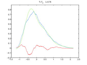
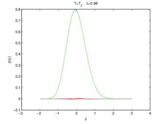
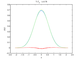
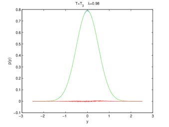
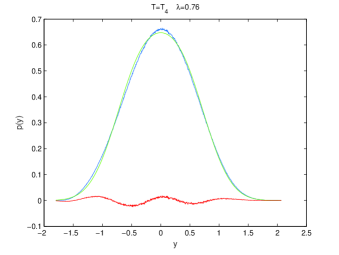
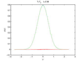
First we look at uncoupled Chebyshev maps of order N=2,3,4𝑁234N=2,3,4 acting as a deterministic chaotic driving force. In our numerical experiment the map (1) is iterated 3Γ—1073superscript1073\times 10^{7} times. In Figs 1a-1f, we see that our analytic results, Eqs.(57)57(57), (59)59(59), and (64)64(64), tightly fit the numerical histograms. We can see that the smaller Ο„πœ\tau, the better the coincidence. Figures 1a and 1b show numerical histograms ρ​(y)πœŒπ‘¦\rho(y) (in the physical picture, these are particle velocity distributions) for driving forces generated by T2subscript𝑇2T_{2}, Figures 1c and 1d show the same for T3subscript𝑇3T_{3}, and Figures 1e and 1f for T4subscript𝑇4T_{4}. Note, any disparity between the histograms and the analytic prediction comes from the neglection of the higher order terms of O​(Ο„3/2)𝑂superscript𝜏32O(\tau^{3/2}) in the fits.

Refer to caption
(a)
Refer to caption
(b)
Refer to caption
(c)
Refer to caption
(d)
Refer to caption
(e)
Refer to caption
(f)
Figure 1: Comparison of the numerical results (blue) with the analytic results (green) for T2subscript𝑇2T_{2} (a),(b); T3subscript𝑇3T_{3} (c),(d); T4subscript𝑇4T_{4} (e),(f). The subtractions between these results, denoting the tightness of fit, are shown in red. The results shown are for Ξ»=eβˆ’Ο„=0.76πœ†superscriptπ‘’πœ0.76\lambda=e^{-\tau}=0.76 (a),(c),(e); and Ξ»=eβˆ’Ο„=0.98πœ†superscriptπ‘’πœ0.98\lambda=e^{-\tau}=0.98 (b),(d),(f).

The figure shows the histograms and the theoretical prediction for two values Ξ»=0.76,0.98πœ†0.760.98\lambda=0.76,0.98 so as to illustrate the behavior of the system when Ξ»πœ†\lambda is both further away and closer to 1 (Ο„πœ\tau is further away and closer to 0). Clearly, for Ξ»β†’1β†’πœ†1\lambda\rightarrow 1 there is convergence to a Gaussian, due to the Ο†πœ‘\varphi-mixing property mentioned earlier. We also show the differences between the histograms and our analytic curves, shown in the figure in red. It can be seen that as Ξ»β†’1β†’πœ†1\lambda\rightarrow 1, for all three Chebyshev polynomials the difference becomes smaller and smaller, consistent with convergence to zero.

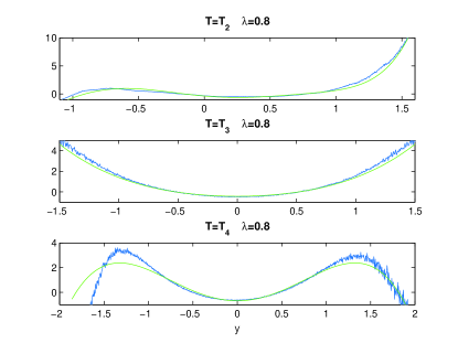
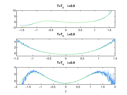
Another interesting aspect of our analytic work in the previous sections was the extraction of the different polynomials that describe the leading order corrections when approaching the Gaussian limit case. These polynomials can be regarded as eigenfunctions of a rescaling operator Ο„β†’12β€‹Ο„β†’πœ12𝜏\tau\to\frac{1}{2}\tau that describes the approach to the Gaussian limit case under rescaling of the parameter Ο„πœ\tau, in the vicinity of the Gaussian fixed point. For T2subscript𝑇2T_{2} we obtain after re-arranging

(Ο€2​ρ​(y)eβˆ’2​y2βˆ’1)​1Ο„=83​y3βˆ’2​y+τ​(329​y6βˆ’313​y4+152​y2βˆ’3748)+O​(Ο„)πœ‹2πœŒπ‘¦superscript𝑒2superscript𝑦211𝜏83superscript𝑦32π‘¦πœ329superscript𝑦6313superscript𝑦4152superscript𝑦23748π‘‚πœ\left(\frac{\sqrt{\frac{\pi}{2}}\rho(y)}{e^{-2y^{2}}}-1\right)\frac{1}{\sqrt{\tau}}=\frac{8}{3}y^{3}-2y+\sqrt{\tau}\left(\frac{32}{9}y^{6}-\frac{31}{3}y^{4}+\frac{15}{2}y^{2}-\frac{37}{48}\right)+O(\tau) (65)

so if we choose for ρ​(y)πœŒπ‘¦\rho(y) a numerically generated histogram one can extract the polynomials by the above re-arrangement. This is shown in Figs 2a and 2b, taking for ρ​(y)πœŒπ‘¦\rho(y) the numerically obtained histogram and two different values of Ο„πœ\tau. Excellent agreement between numerical results and our analytic predictions is obtained for Ο„πœ\tau small. Similarly, we obtain for T3subscript𝑇3T_{3}

(Ο€2​ρ​(y)eβˆ’2​y2βˆ’1)​1Ο„=13​y4+32​y2βˆ’716+O​(Ο„)πœ‹2πœŒπ‘¦superscript𝑒2superscript𝑦211𝜏13superscript𝑦432superscript𝑦2716π‘‚πœ\left(\frac{\sqrt{\frac{\pi}{2}}\rho(y)}{e^{-2y^{2}}}-1\right)\frac{1}{\tau}=\frac{1}{3}y^{4}+\frac{3}{2}y^{2}-\frac{7}{16}+O(\tau) (66)

and for T4subscript𝑇4T_{4}

(Ο€2​ρ​(y)eβˆ’2​y2βˆ’1)​1Ο„=βˆ’y4+7​y22βˆ’1116+O​(Ο„1/2)πœ‹2πœŒπ‘¦superscript𝑒2superscript𝑦211𝜏superscript𝑦47superscript𝑦221116𝑂superscript𝜏12\left(\frac{\sqrt{\frac{\pi}{2}}\rho(y)}{e^{-2y^{2}}}-1\right)\frac{1}{\tau}=-y^{4}+\frac{7y^{2}}{2}-\frac{11}{16}+O(\tau^{1/2}) (67)

Figs 2a, 2b confirm the analytically calculated polynomial form of the leading correction terms for T2,T3,T4subscript𝑇2subscript𝑇3subscript𝑇4T_{2},T_{3},T_{4}, and as expected the deviations from the calculated polynomials (the higher order terms) become very small for small Ο„πœ\tau. For these simulations, we iterated the map (1) 1.75Γ—1071.75superscript1071.75\times 10^{7} times.

Refer to caption
(a)
Refer to caption
(b)
Figure 2: Leading-order corrections to the Gaussian limit case for Ξ»=eβˆ’Ο„=0.8πœ†superscriptπ‘’πœ0.8\lambda=e^{-\tau}=0.8 (a), and Ξ»=eβˆ’Ο„=0.9πœ†superscriptπ‘’πœ0.9\lambda=e^{-\tau}=0.9 (b). The numerical results are shown in blue and the calculated polynomials are shown in green. The Chebyshev map that each plot relates to is demarcated in the plot.

Finally, we may ask what happens if the Chebyshev maps that drive the system are coupled. Here we use diffusively coupled map lattices of the form

xn+1(i)=(1βˆ’Ξ±)​TN​(xn(i))+12​α​(TN​(xn(iβˆ’1))+TN​(xn(i+1))),superscriptsubscriptπ‘₯𝑛1𝑖1𝛼subscript𝑇𝑁superscriptsubscriptπ‘₯𝑛𝑖12𝛼subscript𝑇𝑁superscriptsubscriptπ‘₯𝑛𝑖1subscript𝑇𝑁superscriptsubscriptπ‘₯𝑛𝑖1x_{n+1}^{(i)}=(1-\alpha)T_{N}(x_{n}^{(i)})+\frac{1}{2}\alpha(T_{N}(x_{n}^{(i-1)})+T_{N}(x_{n}^{(i+1)})), (68)

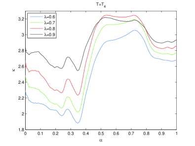
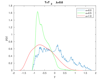
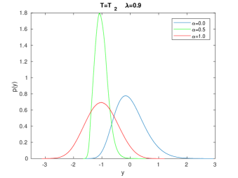
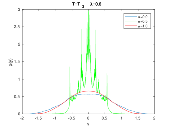
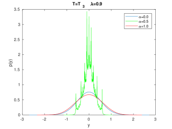
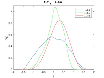
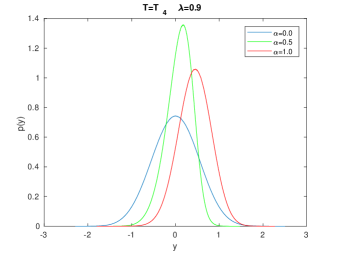
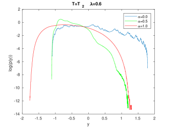
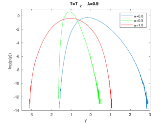
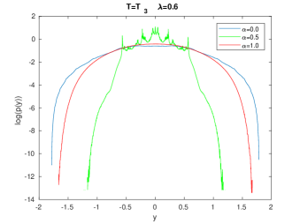
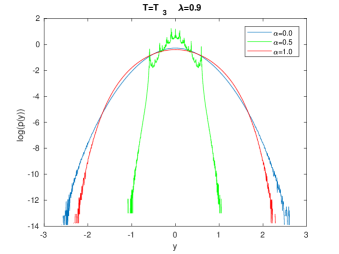
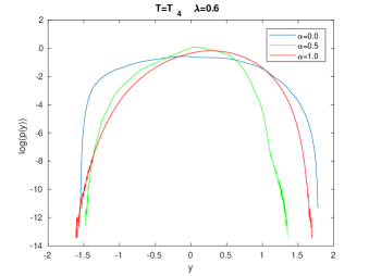
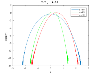
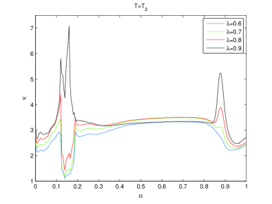
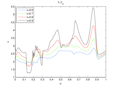
with periodic boundary conditions and lattices of size 1000. For large couplings α𝛼\alpha these systems may lose the Ο†πœ‘\varphi-mixing property, hence convergence to a Gaussian process is not guaranteed anymore if components of this coupled map lattice drive the linear relaxation dynamics. In fact for finite Ο„πœ\tau many complicated shapes of densities can be created. To quantitatively measure the deviation from a Gaussian, Figs 3a-3c show the kurtosis ΞΊπœ…\kappa of the numerically obtained histograms ρ​(y)πœŒπ‘¦\rho(y) as a function of the coupling α𝛼\alpha, with α∈[0,1]𝛼01\alpha\in[0,1], and Δ​α=.005Δ𝛼.005\Delta\alpha=.005, for various values of Ο„πœ\tau. All lattice sites were used as driving forces, iterated 105superscript10510^{5} times giving 108superscript10810^{8} data points, and all the driven velocities were put into the same histogram. This was done for Ξ»=0.6,0.7,0.8,0.9πœ†0.60.70.80.9\lambda=0.6,0.7,0.8,0.9. Some example densities are shown in Figs 4a-4f. Further, the log-plots of these densities are also shown in Figs 5a-5f. These were simulated with 2Γ—1052superscript1052\times 10^{5} iterations giving 2Γ—1082superscript1082\times 10^{8} data points for Ξ±=0.0,0.5,1.0𝛼0.00.51.0\alpha=0.0,0.5,1.0 and Ξ»=0.6,0.9πœ†0.60.9\lambda=0.6,0.9. These plots nicely illustrate the deviation from a Gaussian as the semi-logarithmic plot of a Gaussian is a parabola. Convergence to the Gaussian limit case (with has ΞΊ=3πœ…3\kappa=3) is mathematically rigorously proven for Ξ±=0𝛼0\alpha=0 only. The other cases of α𝛼\alpha can lead to more complex non-Gaussian behavior due to strong temporal correlations of the iterates, where the ordinary central limit behavior is not guaranteed anymore Tirn . An interesting example is the case of T3subscript𝑇3T_{3} with Ξ±=0.5𝛼0.5\alpha=0.5 where our numerics indicates that complex non-Gaussian behavior seems to persist even for Ο„β†’0β†’πœ0\tau\to 0. In the quantum field theoretical applications described in Beck7 -SM this corresponds to a strongly interacting field theory rather than a free field.
Refer to caption
(a)
Refer to caption
(b)
Refer to caption
(c)
Figure 3: Kurtosis ΞΊπœ…\kappa of the velocity distributons as a function of the couplings α𝛼\alpha. Each plot corresponds to a different Chebyshev polynomial being coupled: T2subscript𝑇2T_{2} (a), T3subscript𝑇3T_{3} (b), T4subscript𝑇4T_{4} (c). The blue lines describe Ξ»=0.6πœ†0.6\lambda=0.6, green describes Ξ»=0.7πœ†0.7\lambda=0.7, red describes Ξ»=0.8πœ†0.8\lambda=0.8, and black describes Ξ»=0.9πœ†0.9\lambda=0.9. Δ​α=.005Δ𝛼.005\Delta\alpha=.005. For some parameter values α𝛼\alpha, there are particularly strong deviations of the kurtosis from the Gaussian value ΞΊ=3πœ…3\kappa=3.
Refer to caption
(a)
Refer to caption
(b)
Refer to caption
(c)
Refer to caption
(d)
Refer to caption
(e)
Refer to caption
(f)
Figure 4: Numerical results of particle velocity distributions for driving forces given by diffusively coupled map lattices with couplings Ξ±=0𝛼0\alpha=0 (blue), Ξ±=0.5𝛼0.5\alpha=0.5 (green), and Ξ±=1𝛼1\alpha=1 (red), for T2subscript𝑇2T_{2} (a),(b); T3subscript𝑇3T_{3} (c),(d); T4subscript𝑇4T_{4} (e),(f). The results shown are for Ξ»=eβˆ’Ο„=0.6πœ†superscriptπ‘’πœ0.6\lambda=e^{-\tau}=0.6 (a),(c),(e); and Ξ»=eβˆ’Ο„=0.9πœ†superscriptπ‘’πœ0.9\lambda=e^{-\tau}=0.9 (b),(d),(f).
Refer to caption
(a)
Refer to caption
(b)
Refer to caption
(c)
Refer to caption
(d)
Refer to caption
(e)
Refer to caption
(f)
Figure 5: Same as Fig.Β 4 but in a log-linear plot. In such a plot the Gaussian shape corresponds to a parabola.

VIII Conclusion

In this paper we have studied deterministic chaotic analogues of stochastic differential equations, where the Gaussian white noise of the stochastic differential equation is replaced by deterministic chaotic maps, evolving on a small time scale Ο„πœ\tau. We have done a perturbative expansion of the Perron-Frobenius equation of this problem, and compared terms of equal power in Ο„πœ\sqrt{\tau} on both sides of the equation (a method similar to van Kampen’s omega expansion Kampen for stochastic systems but here applied in a dynamical systems context). The result are functional equations which are difficult to solve. However, for Chebyshev maps of order N𝑁N we were able to find explicit solutions for arbitrary N𝑁N. The results demonstrate that a highly nontrivial mathematical structure arises where the approach to the Gaussian limit case is different for each of the Chebyshev maps T2subscript𝑇2T_{2}, T3subscript𝑇3T_{3}, T4subscript𝑇4T_{4}. However, for Nβ‰₯4𝑁4N\geq 4 the leading order correction to the Gaussian is the same for all higher Chebyshev maps TNsubscript𝑇𝑁T_{N} with Nβ‰₯4𝑁4N\geq 4. The extracted polynomial functions in the perturbative expansion of the invariant density can be regarded as eigenfunctions of a rescaling operator Ο„β†’12β€‹Ο„β†’πœ12𝜏\tau\to\frac{1}{2}\tau that describes via which route the Gaussian limit case is approached under successive rescaling of the time scale parameter. The leading order approach to the Gaussian limit case is of order O​(Ο„1/2)𝑂superscript𝜏12O(\tau^{1/2}) for T2subscript𝑇2T_{2} and of order O​(Ο„)π‘‚πœO(\tau) for Nβ‰₯3𝑁3N\geq 3, though with different polynomial functional forms for T3subscript𝑇3T_{3} and T4subscript𝑇4T_{4}. Our results have applications in quantum field theoretical models Beck7 in which the Gaussian white noise of the Parisis-Wu approach of stochastic quantization is replaced by a deterministic chaotic dynamics on a small but finite time scale.

IX Appendix A

Continuing from Eq. (51) in Section IV, we can evaluate the left-hand side of the inhomogeneous Fokker-Planck equation (42)42(42):

βˆ«π‘‘x​x​b​(x,y,t)=⟨x2βŸ©β€‹Ξ²1​(y,t)=12​(2Ο€)1/2​(1βˆ’4​y2)​eβˆ’2​y2differential-dπ‘₯π‘₯𝑏π‘₯𝑦𝑑delimited-⟨⟩superscriptπ‘₯2subscript𝛽1𝑦𝑑12superscript2πœ‹1214superscript𝑦2superscript𝑒2superscript𝑦2\int dx\ xb(x,y,t)=\langle x^{2}\rangle\beta_{1}(y,t)=\frac{1}{2}\left(\frac{2}{\pi}\right)^{1/2}(1-4y^{2})e^{-2y^{2}} (69)

The stationary solution of Eq. (42)42(42) satisfies

βˆ‚βˆ‚y​α​(y)+4​y​α​(y)=2​(2Ο€)1/2​(1βˆ’4​y2)​eβˆ’2​y2+c​o​n​s​t𝑦𝛼𝑦4𝑦𝛼𝑦2superscript2πœ‹1214superscript𝑦2superscript𝑒2superscript𝑦2π‘π‘œπ‘›π‘ π‘‘\frac{\partial}{\partial y}\alpha(y)+4y\alpha(y)=2\left(\frac{2}{\pi}\right)^{1/2}(1-4y^{2})e^{-2y^{2}}+const (70)

In general, all solutions of the first-order linear differential equation

βˆ‚βˆ‚y​α+g​(y)​α+f​(y)=0𝑦𝛼𝑔𝑦𝛼𝑓𝑦0\frac{\partial}{\partial y}\alpha+g(y)\alpha+f(y)=0 (71)

are given by

α​(y)=eβˆ’G​(y)​[Cβˆ’βˆ«1f​(y)​eG​(y)]𝛼𝑦superscript𝑒𝐺𝑦delimited-[]𝐢subscript1𝑓𝑦superscript𝑒𝐺𝑦\alpha(y)=e^{-G(y)}\left[C-\int_{1}f(y)e^{G(y)}\right] (72)

Here G𝐺G is an indefinite integral of g𝑔g,

βˆ‚βˆ‚y​G​(y)=g​(y)𝑦𝐺𝑦𝑔𝑦\frac{\partial}{\partial y}G(y)=g(y) (73)

and ∫1…subscript1…\int_{1}\dots denotes an indefinite integral of the argument. In our case

g​(y)=4​y𝑔𝑦4𝑦g(y)=4y (74)
f​(y)=2​(2Ο€)1/2​(4​y2βˆ’1)​eβˆ’2​y2βˆ’c​o​n​s​t𝑓𝑦2superscript2πœ‹124superscript𝑦21superscript𝑒2superscript𝑦2π‘π‘œπ‘›π‘ π‘‘f(y)=2\left(\frac{2}{\pi}\right)^{1/2}(4y^{2}-1)e^{-2y^{2}}-const (75)

This yields

G​(y)=2​y2𝐺𝑦2superscript𝑦2G(y)=2y^{2} (76)
α​(y)=eβˆ’2​y2​[Cβˆ’2​(2Ο€)1/2β€‹βˆ«1(4​y2βˆ’1)+c​o​n​s​tβ€‹βˆ«1e2​y2]𝛼𝑦superscript𝑒2superscript𝑦2delimited-[]𝐢2superscript2πœ‹12subscript14superscript𝑦21π‘π‘œπ‘›π‘ π‘‘subscript1superscript𝑒2superscript𝑦2\alpha(y)=e^{-2y^{2}}\left[C-2\left(\frac{2}{\pi}\right)^{1/2}\int_{1}(4y^{2}-1)+const\int_{1}e^{2y^{2}}\right] (77)

For C𝐢C=const=0 we obtain

α​(y)=(2Ο€)1/2​eβˆ’2​y2​(2​yβˆ’83​y3)𝛼𝑦superscript2πœ‹12superscript𝑒2superscript𝑦22𝑦83superscript𝑦3\alpha(y)=\left(\frac{2}{\pi}\right)^{1/2}e^{-2y^{2}}\left(2y-\frac{8}{3}y^{3}\right) (78)

To obtain the second-order correction term, we have to solve the coupled system of equations (43)43(43) and (45)45(45). Putting Eq. (47)47(47) into Eq. (45)45(45) and again using the symmetry of the pre-images of T𝑇T, we can write Eq. (45)45(45) as

c​(xβ€²,y,t)=𝑐superscriptπ‘₯′𝑦𝑑absent\displaystyle c(x^{\prime},y,t)={} βˆ‘x∈Tβˆ’1​(xβ€²)1|T′​(x)|{c(x,y,t)\displaystyle\sum_{x\in T^{-1}(x^{\prime})}\frac{1}{|T^{\prime}(x)|}\bigg{\{}c(x,y,t) (79)
+(1βˆ’2x2)h(x)[12βˆ‚βˆ‚yΞ²1(y,t)βˆ’14βˆ‚2βˆ‚y2Ξ±(y,t)]}\displaystyle+(1-2x^{2})h(x)\left[\frac{1}{2}\frac{\partial}{\partial y}\beta_{1}(y,t)-\frac{1}{4}\frac{\partial^{2}}{\partial y^{2}}\alpha(y,t)\right]\bigg{\}}

Similarly as Eq. (44)44(44), this equation is solved by the ansatz

c​(x,y,t)=h​(x)​γ0​(y,t)+x​h​(x)​γ1​(y,t)𝑐π‘₯π‘¦π‘‘β„Žπ‘₯subscript𝛾0𝑦𝑑π‘₯β„Žπ‘₯subscript𝛾1𝑦𝑑c(x,y,t)=h(x)\gamma_{0}(y,t)+xh(x)\gamma_{1}(y,t) (80)

We obtain Ξ³0​(y,t)subscript𝛾0𝑦𝑑\gamma_{0}(y,t) arbitrary and

Ξ³1​(y,t)=12β€‹βˆ‚βˆ‚y​β1​(y,t)βˆ’14β€‹βˆ‚2βˆ‚y2​α​(y,t)subscript𝛾1𝑦𝑑12𝑦subscript𝛽1𝑦𝑑14superscript2superscript𝑦2𝛼𝑦𝑑\gamma_{1}(y,t)=\frac{1}{2}\frac{\partial}{\partial y}\beta_{1}(y,t)-\frac{1}{4}\frac{\partial^{2}}{\partial y^{2}}\alpha(y,t) (81)

Putting Eqs. (81)81(81), (47)47(47), and (50)50(50) into Eq. (43)43(43), we arrive at the following equation for the unknown function Ξ²0​(y,t)=β​(y,t)subscript𝛽0𝑦𝑑𝛽𝑦𝑑\beta_{0}(y,t)=\beta(y,t):

0=0absent\displaystyle 0={} βˆ‚βˆ‚y​(y​β​(y,t))+14β€‹βˆ‚2βˆ‚y2​β​(y,t)βˆ’βˆ‚βˆ‚t​β​(y,t)𝑦𝑦𝛽𝑦𝑑14superscript2superscript𝑦2𝛽𝑦𝑑𝑑𝛽𝑦𝑑\displaystyle\frac{\partial}{\partial y}(y\beta(y,t))+\frac{1}{4}\frac{\partial^{2}}{\partial y^{2}}\beta(y,t)-\frac{\partial}{\partial t}\beta(y,t) (82)
+[12yβˆ‚βˆ‚y+12(y2+1)βˆ‚2βˆ‚y2+14yβˆ‚3βˆ‚y3+564βˆ‚4βˆ‚y4\displaystyle+\biggl{[}\frac{1}{2}y\frac{\partial}{\partial y}+\frac{1}{2}(y^{2}+1)\frac{\partial^{2}}{\partial y^{2}}+\frac{1}{4}y\frac{\partial^{3}}{\partial y^{3}}+\frac{5}{64}\frac{\partial^{4}}{\partial y^{4}}
βˆ’12+βˆ‚βˆ‚tβˆ’12βˆ‚2βˆ‚t2]p0(y,t)+18βˆ‚3βˆ‚y3Ξ±(y,t)\displaystyle-\frac{1}{2}+\frac{\partial}{\partial t}-\frac{1}{2}\frac{\partial^{2}}{\partial t^{2}}\biggr{]}p_{0}(y,t)+\frac{1}{8}\frac{\partial^{3}}{\partial y^{3}}\alpha(y,t)

In the stationary case, we can use Eqs. (46)46(46) and (79)79(79) to obtain

0=βˆ‚βˆ‚y​(y​β​(y))+14β€‹βˆ‚2βˆ‚y2​β​(y)+(2Ο€)1/2​(643​y6βˆ’68​y4+46​y2βˆ’154)​eβˆ’2​y20𝑦𝑦𝛽𝑦14superscript2superscript𝑦2𝛽𝑦superscript2πœ‹12643superscript𝑦668superscript𝑦446superscript𝑦2154superscript𝑒2superscript𝑦20=\frac{\partial}{\partial y}(y\beta(y))+\frac{1}{4}\frac{\partial^{2}}{\partial y^{2}}\beta(y)+\left(\frac{2}{\pi}\right)^{1/2}\left(\frac{64}{3}y^{6}-68y^{4}+46y^{2}-\frac{15}{4}\right)e^{-2y^{2}} (83)

One can easily check that this differential equation is solved by

β​(y)=(2Ο€)1/2​(329​y6βˆ’313​y4+152​y2βˆ’3748)​eβˆ’2​y2𝛽𝑦superscript2πœ‹12329superscript𝑦6313superscript𝑦4152superscript𝑦23748superscript𝑒2superscript𝑦2\beta(y)=\left(\frac{2}{\pi}\right)^{1/2}\left(\frac{32}{9}y^{6}-\frac{31}{3}y^{4}+\frac{15}{2}y^{2}-\frac{37}{48}\right)e^{-2y^{2}} (84)

X Appendix B

Continuing from Eq. (58) in Section V, and using Lemma 4 in Appendix C, for Nβ‰₯3𝑁3N\geq 3, (58)58(58) reduces to

b​(xβ€²,y,t)=βˆ‘x∈Tβˆ’1​(xβ€²)1|T′​(x)|​b​(x,y,t)𝑏superscriptπ‘₯′𝑦𝑑subscriptπ‘₯superscript𝑇1superscriptπ‘₯β€²1superscript𝑇′π‘₯𝑏π‘₯𝑦𝑑b(x^{\prime},y,t)=\sum_{x\in T^{-1}(x^{\prime})}\frac{1}{|T^{\prime}(x)|}b(x,y,t) (85)

which is solved by b​(x,y,t)=h​(x)​β​(y,t)𝑏π‘₯π‘¦π‘‘β„Žπ‘₯𝛽𝑦𝑑b(x,y,t)=h(x)\beta(y,t).

The integrated equations reduce for any Chebyshev map with Nβ‰₯2𝑁2N\geq 2 as follows. Since

βˆ«π‘‘x​x​φ​(x,y,t)=⟨xβŸ©β€‹p0​(y,t)differential-dπ‘₯π‘₯πœ‘π‘₯𝑦𝑑delimited-⟨⟩π‘₯subscript𝑝0𝑦𝑑\int dx\ x\ \varphi(x,y,t)=\langle x\rangle p_{0}(y,t) (86)

and

βˆ«π‘‘x​x​a​(x,y,t)=⟨xβŸ©β€‹Ξ±β€‹(y,t)differential-dπ‘₯π‘₯π‘Žπ‘₯𝑦𝑑delimited-⟨⟩π‘₯𝛼𝑦𝑑\int dx\ x\ a(x,y,t)=\langle x\rangle\alpha(y,t) (87)

(as per the definition of the first moment, and implied by (21)21(21) and (22)22(22)), we have

(26)β‡”βŸ¨x⟩=0⇔26delimited-⟨⟩π‘₯0(26)\Leftrightarrow\langle x\rangle=0
(27)β‡”βˆ‚βˆ‚y​(y​p0​(y,t))+14β€‹βˆ‚2βˆ‚y2​p0​(y,t)βˆ’βˆ‚βˆ‚t​p0​(y,t)=0⇔27𝑦𝑦subscript𝑝0𝑦𝑑14superscript2superscript𝑦2subscript𝑝0𝑦𝑑𝑑subscript𝑝0𝑦𝑑0(27)\Leftrightarrow\frac{\partial}{\partial y}\left(yp_{0}(y,t)\right)+\frac{1}{4}\frac{\partial^{2}}{\partial y^{2}}p_{0}(y,t)-\frac{\partial}{\partial t}p_{0}(y,t)=0

(the Fokker-Planck equation), and

(28)⇔⇔28absent\displaystyle(28)\Leftrightarrow βˆ‚βˆ‚yβ€‹βˆ«π‘‘x​x​b​(x,y,t)𝑦differential-dπ‘₯π‘₯𝑏π‘₯𝑦𝑑\displaystyle\frac{\partial}{\partial y}\int dx\ x\ b(x,y,t)
=\displaystyle= βˆ‚βˆ‚y​(y​α​(y,t))+14β€‹βˆ‚2βˆ‚y2​α​(y,t)βˆ’βˆ‚βˆ‚t​α​(y,t)𝑦𝑦𝛼𝑦𝑑14superscript2superscript𝑦2𝛼𝑦𝑑𝑑𝛼𝑦𝑑\displaystyle\frac{\partial}{\partial y}\left(y\alpha(y,t)\right)+\frac{1}{4}\frac{\partial^{2}}{\partial y^{2}}\alpha(y,t)-\frac{\partial}{\partial t}\alpha(y,t)

(an inhomogeneous Fokker-Planck equation). As previously shown, for N=2𝑁2N=2 we have

b​(x,y,t)=h​(x)​β0​(y,t)+x​h​(x)​β1​(y,t)𝑏π‘₯π‘¦π‘‘β„Žπ‘₯subscript𝛽0𝑦𝑑π‘₯β„Žπ‘₯subscript𝛽1𝑦𝑑b(x,y,t)=h(x)\beta_{0}(y,t)+xh(x)\beta_{1}(y,t) (88)

and (28)28(28) becomes (56)56(56)

βˆ‚βˆ‚y​(y​α​(y,t))+14β€‹βˆ‚2βˆ‚y2​α​(y,t)βˆ’βˆ‚βˆ‚t​α​(y,t)=βˆ’18β€‹βˆ‚3βˆ‚y3​p0​(y,t)𝑦𝑦𝛼𝑦𝑑14superscript2superscript𝑦2𝛼𝑦𝑑𝑑𝛼𝑦𝑑18superscript3superscript𝑦3subscript𝑝0𝑦𝑑\frac{\partial}{\partial y}\left(y\alpha(y,t)\right)+\frac{1}{4}\frac{\partial^{2}}{\partial y^{2}}\alpha(y,t)-\frac{\partial}{\partial t}\alpha(y,t)=-\frac{1}{8}\frac{\partial^{3}}{\partial y^{3}}p_{0}(y,t)

For Nβ‰₯3𝑁3N\geq 3, we have

b​(x,y,t)=h​(x)​β​(y,t)𝑏π‘₯π‘¦π‘‘β„Žπ‘₯𝛽𝑦𝑑b(x,y,t)=h(x)\beta(y,t)

hence

βˆ«π‘‘x​x​b​(x,y,t)=⟨xβŸ©β€‹Ξ²β€‹(y,t)=0differential-dπ‘₯π‘₯𝑏π‘₯𝑦𝑑delimited-⟨⟩π‘₯𝛽𝑦𝑑0\int dx\ xb(x,y,t)=\langle x\rangle\beta(y,t)=0

hence (28) then reads

βˆ‚βˆ‚y(yΞ±(y,t)+14βˆ‚2βˆ‚y2Ξ±(y,t)βˆ’βˆ‚βˆ‚tΞ±(y,t)=0\frac{\partial}{\partial y}(y\alpha(y,t)+\frac{1}{4}\frac{\partial^{2}}{\partial y^{2}}\alpha(y,t)-\frac{\partial}{\partial t}\alpha(y,t)=0

which is a Fokker-Planck equation. Now, (29)29(29) reduces to

βˆ‚βˆ‚yβ€‹βˆ«π‘‘x​x​c​(x,y,t)=𝑦differential-dπ‘₯π‘₯𝑐π‘₯𝑦𝑑absent\displaystyle\frac{\partial}{\partial y}\int dx\ xc(x,y,t)= βˆ‚βˆ‚y​(y​β​(y,t))+14β€‹βˆ‚2βˆ‚y2​β​(y,t)βˆ’βˆ‚βˆ‚t​β​(y,t)𝑦𝑦𝛽𝑦𝑑14superscript2superscript𝑦2𝛽𝑦𝑑𝑑𝛽𝑦𝑑\displaystyle\frac{\partial}{\partial y}\left(y\beta(y,t)\right)+\frac{1}{4}\frac{\partial^{2}}{\partial y^{2}}\beta(y,t)-\frac{\partial}{\partial t}\beta(y,t) (89)
+(βˆ’12+βˆ‚βˆ‚tβˆ’12β€‹βˆ‚2βˆ‚t2+12​yβ€‹βˆ‚βˆ‚y+12​(y2+1)β€‹βˆ‚2βˆ‚y2+14​yβ€‹βˆ‚3βˆ‚y3+164β€‹βˆ‚4βˆ‚y4)​eβˆ’2​y2​2Ο€12𝑑12superscript2superscript𝑑212𝑦𝑦12superscript𝑦21superscript2superscript𝑦214𝑦superscript3superscript𝑦3164superscript4superscript𝑦4superscript𝑒2superscript𝑦22πœ‹\displaystyle+\left(-\frac{1}{2}+\frac{\partial}{\partial t}-\frac{1}{2}\frac{\partial^{2}}{\partial t^{2}}+\frac{1}{2}y\frac{\partial}{\partial y}+\frac{1}{2}(y^{2}+1)\frac{\partial^{2}}{\partial y^{2}}+\frac{1}{4}y\frac{\partial^{3}}{\partial y^{3}}+\frac{1}{64}\frac{\partial^{4}}{\partial y^{4}}\right)e^{-2y^{2}}\sqrt{\frac{2}{\pi}}
=\displaystyle= βˆ‚βˆ‚y​(y​β​(y,t))+14β€‹βˆ‚2βˆ‚y2​β​(y,t)βˆ’βˆ‚βˆ‚t​β​(y,t)βˆ’2π​(74βˆ’10​y2+4​y4)​eβˆ’2​y2𝑦𝑦𝛽𝑦𝑑14superscript2superscript𝑦2𝛽𝑦𝑑𝑑𝛽𝑦𝑑2πœ‹7410superscript𝑦24superscript𝑦4superscript𝑒2superscript𝑦2\displaystyle\frac{\partial}{\partial y}\left(y\beta(y,t)\right)+\frac{1}{4}\frac{\partial^{2}}{\partial y^{2}}\beta(y,t)-\frac{\partial}{\partial t}\beta(y,t)-\sqrt{\frac{2}{\pi}}\left(\frac{7}{4}-10y^{2}+4y^{4}\right)e^{-2y^{2}}

with Ξ²=Ξ²0𝛽subscript𝛽0\beta=\beta_{0} and Ξ²1=0subscript𝛽10\beta_{1}=0. c​(x,y,t)𝑐π‘₯𝑦𝑑c(x,y,t) satisfies Eq. (18)18(18), which for Nβ‰₯3𝑁3N\geq 3 can be written as

c​(xβ€²,y,t)=βˆ‘x∈Tβˆ’1​(xβ€²)1|T′​(x)|​[c​(x,y,t)+14​h​(x)​(2​x2βˆ’1)β€‹βˆ‚2βˆ‚y2​α​(y,t)βˆ’16​x3​h​(x)β€‹βˆ‚3βˆ‚y3​p0​(y,t)]𝑐superscriptπ‘₯′𝑦𝑑subscriptπ‘₯superscript𝑇1superscriptπ‘₯β€²1superscript𝑇′π‘₯delimited-[]𝑐π‘₯𝑦𝑑14β„Žπ‘₯2superscriptπ‘₯21superscript2superscript𝑦2𝛼𝑦𝑑16superscriptπ‘₯3β„Žπ‘₯superscript3superscript𝑦3subscript𝑝0𝑦𝑑c(x^{\prime},y,t)=\sum_{x\in T^{-1}(x^{\prime})}\frac{1}{|T^{\prime}(x)|}\left[c(x,y,t)+\frac{1}{4}h(x)(2x^{2}-1)\frac{\partial^{2}}{\partial y^{2}}\alpha(y,t)-\frac{1}{6}x^{3}h(x)\frac{\partial^{3}}{\partial y^{3}}p_{0}(y,t)\right] (90)

using Lemmas 2 and 3 in Appendix C and the Fokker-Planck equation for α​(y,t)𝛼𝑦𝑑\alpha(y,t).

Using Lemma 4 in Appendix C, (90)90(90) even further reduces to

c​(xβ€²,y,t)=βˆ‘x∈Tβˆ’1​(xβ€²)1|T′​(x)|​[c​(x,y,t)βˆ’16​x3​h​(x)β€‹βˆ‚3βˆ‚y3​p0​(y,t)]𝑐superscriptπ‘₯′𝑦𝑑subscriptπ‘₯superscript𝑇1superscriptπ‘₯β€²1superscript𝑇′π‘₯delimited-[]𝑐π‘₯𝑦𝑑16superscriptπ‘₯3β„Žπ‘₯superscript3superscript𝑦3subscript𝑝0𝑦𝑑c(x^{\prime},y,t)=\sum_{x\in T^{-1}(x^{\prime})}\frac{1}{|T^{\prime}(x)|}\left[c(x,y,t)-\frac{1}{6}x^{3}h(x)\frac{\partial^{3}}{\partial y^{3}}p_{0}(y,t)\right] (91)

Similar to b​(x,y,t)𝑏π‘₯𝑦𝑑b(x,y,t) for T2subscript𝑇2T_{2}, we will choose the ansatz for solutions of Eq. (91)91(91) as:

c​(x,y,t)𝑐π‘₯𝑦𝑑\displaystyle c(x,y,t) =h​(x)​γ0​(y,t)+x​h​(x)​γ1​(y,t)absentβ„Žπ‘₯subscript𝛾0𝑦𝑑π‘₯β„Žπ‘₯subscript𝛾1𝑦𝑑\displaystyle=h(x)\gamma_{0}(y,t)+xh(x)\gamma_{1}(y,t) (92)
β‡’β‡’\displaystyle\Rightarrow l=h​(xβ€²)​γ0​(y,t)+x′​h​(xβ€²)​γ1​(y,t)π‘™β„Žsuperscriptπ‘₯β€²subscript𝛾0𝑦𝑑superscriptπ‘₯β€²β„Žsuperscriptπ‘₯β€²subscript𝛾1𝑦𝑑\displaystyle l=h(x^{\prime})\gamma_{0}(y,t)+x^{\prime}h(x^{\prime})\gamma_{1}(y,t)

where xβ€²=4​x3βˆ’3​xsuperscriptπ‘₯β€²4superscriptπ‘₯33π‘₯x^{\prime}=4x^{3}-3x. This gives

=Ξ³0​(y,t)​(βˆ‘x∈Tβˆ’1​(xβ€²)h​(x)|T′​(x)|)+Ξ³1​(y,t)β€‹βˆ‘x∈Tβˆ’1​(xβ€²)(4​x3βˆ’3​x)​h​(x)|T′​(x)|absentsubscript𝛾0𝑦𝑑subscriptπ‘₯superscript𝑇1superscriptπ‘₯β€²β„Žπ‘₯superscript𝑇′π‘₯subscript𝛾1𝑦𝑑subscriptπ‘₯superscript𝑇1superscriptπ‘₯β€²4superscriptπ‘₯33π‘₯β„Žπ‘₯superscript𝑇′π‘₯\displaystyle=\gamma_{0}(y,t)\left(\sum_{x\in T^{-1}(x^{\prime})}\frac{h(x)}{|T^{\prime}(x)|}\right)+\gamma_{1}(y,t)\sum_{x\in T^{-1}(x^{\prime})}(4x^{3}-3x)\frac{h(x)}{|T^{\prime}(x)|} (93)
=βˆ‘x∈Tβˆ’1​(xβ€²)h​(x)|T′​(x)|​(Ξ³0​(y,t)+4​x3​γ1​(y,t))absentsubscriptπ‘₯superscript𝑇1superscriptπ‘₯β€²β„Žπ‘₯superscript𝑇′π‘₯subscript𝛾0𝑦𝑑4superscriptπ‘₯3subscript𝛾1𝑦𝑑\displaystyle=\sum_{x\in T^{-1}(x^{\prime})}\frac{h(x)}{|T^{\prime}(x)|}\left(\gamma_{0}(y,t)+4x^{3}\gamma_{1}(y,t)\right)

by Lemma 3 in Appendix C.

r=π‘Ÿabsent\displaystyle r= βˆ‘x∈Tβˆ’1​(xβ€²)1|T′​(x)|​[h​(x)​γ0​(y,t)+x​h​(x)​γ1​(y,t)βˆ’16​x3​h​(x)β€‹βˆ‚3βˆ‚y3​p0​(y,t)]subscriptπ‘₯superscript𝑇1superscriptπ‘₯β€²1superscript𝑇′π‘₯delimited-[]β„Žπ‘₯subscript𝛾0𝑦𝑑π‘₯β„Žπ‘₯subscript𝛾1𝑦𝑑16superscriptπ‘₯3β„Žπ‘₯superscript3superscript𝑦3subscript𝑝0𝑦𝑑\displaystyle\sum_{x\in T^{-1}(x^{\prime})}\frac{1}{|T^{\prime}(x)|}\left[h(x)\gamma_{0}(y,t)+xh(x)\gamma_{1}(y,t)-\frac{1}{6}x^{3}h(x)\frac{\partial^{3}}{\partial y^{3}}p_{0}(y,t)\right] (94)
=\displaystyle= βˆ‘x∈Tβˆ’1​(xβ€²)h​(x)|T′​(x)|​[Ξ³0​(y,t)βˆ’16​x3β€‹βˆ‚3βˆ‚y3​p0​(y,t)]subscriptπ‘₯superscript𝑇1superscriptπ‘₯β€²β„Žπ‘₯superscript𝑇′π‘₯delimited-[]subscript𝛾0𝑦𝑑16superscriptπ‘₯3superscript3superscript𝑦3subscript𝑝0𝑦𝑑\displaystyle\sum_{x\in T^{-1}(x^{\prime})}\frac{h(x)}{|T^{\prime}(x)|}\left[\gamma_{0}(y,t)-\frac{1}{6}x^{3}\frac{\partial^{3}}{\partial y^{3}}p_{0}(y,t)\right]

When we let l=rπ‘™π‘Ÿl=r we get Ξ³0​(y,t)subscript𝛾0𝑦𝑑\gamma_{0}(y,t) arbitrary and

Ξ³1​(y,t)=subscript𝛾1𝑦𝑑absent\displaystyle\gamma_{1}(y,t)= βˆ’124β€‹βˆ‚3βˆ‚y3​p0​(y,t)124superscript3superscript𝑦3subscript𝑝0𝑦𝑑\displaystyle-\frac{1}{24}\frac{\partial^{3}}{\partial y^{3}}p_{0}(y,t) (95)
=\displaystyle= (2Ο€)1/2​(83​y3βˆ’2​y)​eβˆ’2​y2superscript2πœ‹1283superscript𝑦32𝑦superscript𝑒2superscript𝑦2\displaystyle\left(\frac{2}{\pi}\right)^{1/2}\left(\frac{8}{3}y^{3}-2y\right)e^{-2y^{2}}

Hence

βˆ«π‘‘x​x​c​(x,y,t)=⟨xβŸ©β€‹Ξ³0​(y,t)+⟨x2βŸ©β€‹Ξ³1​(y,t)=(2Ο€)1/2​(43​y3βˆ’y)​eβˆ’2​y2differential-dπ‘₯π‘₯𝑐π‘₯𝑦𝑑delimited-⟨⟩π‘₯subscript𝛾0𝑦𝑑delimited-⟨⟩superscriptπ‘₯2subscript𝛾1𝑦𝑑superscript2πœ‹1243superscript𝑦3𝑦superscript𝑒2superscript𝑦2\int dx\ xc(x,y,t)=\langle x\rangle\gamma_{0}(y,t)+\langle x^{2}\rangle\gamma_{1}(y,t)=\left(\frac{2}{\pi}\right)^{1/2}\left(\frac{4}{3}y^{3}-y\right)e^{-2y^{2}} (96)

(where ⟨x⟩=0delimited-⟨⟩π‘₯0\langle x\rangle=0 and ⟨x2⟩=12delimited-⟨⟩superscriptπ‘₯212\langle x^{2}\rangle=\frac{1}{2}) and

βˆ‚βˆ‚yβ€‹βˆ«π‘‘x​x​c​(x,y,t)=𝑦differential-dπ‘₯π‘₯𝑐π‘₯𝑦𝑑absent\displaystyle\frac{\partial}{\partial y}\int dx\ xc(x,y,t)= (2Ο€)1/2​[(4​y2βˆ’1)​eβˆ’2​y2βˆ’4​y​(43​y3βˆ’y)​eβˆ’2​y2]superscript2πœ‹12delimited-[]4superscript𝑦21superscript𝑒2superscript𝑦24𝑦43superscript𝑦3𝑦superscript𝑒2superscript𝑦2\displaystyle\left(\frac{2}{\pi}\right)^{1/2}\biggl{[}\left(4y^{2}-1\right)e^{-2y^{2}}-4y\left(\frac{4}{3}y^{3}-y\right)e^{-2y^{2}}\biggr{]} (97)
=\displaystyle= (2Ο€)1/2​(βˆ’163​y4+8​y2βˆ’1)​eβˆ’2​y2superscript2πœ‹12163superscript𝑦48superscript𝑦21superscript𝑒2superscript𝑦2\displaystyle\left(\frac{2}{\pi}\right)^{1/2}\left(-\frac{16}{3}y^{4}+8y^{2}-1\right)e^{-2y^{2}}

To this we have to add the Nβ‰₯4𝑁4N\geq 4 contribution (see section VI)

(2Ο€)1/2​(4​y4βˆ’10​y2+74)​eβˆ’2​y2superscript2πœ‹124superscript𝑦410superscript𝑦274superscript𝑒2superscript𝑦2\left(\frac{2}{\pi}\right)^{1/2}\left(4y^{4}-10y^{2}+\frac{7}{4}\right)e^{-2y^{2}} (98)

Hence, for N=3𝑁3N=3, β​(y,t)𝛽𝑦𝑑\beta(y,t) satisfies the inhomogeneous Fokker-Planck equation

βˆ‚βˆ‚y​(y​β​(y,t))+14β€‹βˆ‚2βˆ‚y2​β​(y,t)βˆ’βˆ‚βˆ‚t​β​(y,t)=(2Ο€)1/2​(βˆ’43​y4βˆ’2​y2+34)​eβˆ’2​y2𝑦𝑦𝛽𝑦𝑑14superscript2superscript𝑦2𝛽𝑦𝑑𝑑𝛽𝑦𝑑superscript2πœ‹1243superscript𝑦42superscript𝑦234superscript𝑒2superscript𝑦2\frac{\partial}{\partial y}\left(y\beta(y,t)\right)+\frac{1}{4}\frac{\partial^{2}}{\partial y^{2}}\beta(y,t)-\frac{\partial}{\partial t}\beta(y,t)=\left(\frac{2}{\pi}\right)^{1/2}\left(-\frac{4}{3}y^{4}-2y^{2}+\frac{3}{4}\right)e^{-2y^{2}} (99)

From the ansatz for the stationary solution

β​(y)=Ξ±0​eβˆ’2​y2+Ξ±1​y2​eβˆ’2​y2+Ξ±2​y4​eβˆ’2​y2𝛽𝑦subscript𝛼0superscript𝑒2superscript𝑦2subscript𝛼1superscript𝑦2superscript𝑒2superscript𝑦2subscript𝛼2superscript𝑦4superscript𝑒2superscript𝑦2\beta(y)=\alpha_{0}e^{-2y^{2}}+\alpha_{1}y^{2}e^{-2y^{2}}+\alpha_{2}y^{4}e^{-2y^{2}} (100)

and using βˆ«π‘‘y​β​(y)=0differential-d𝑦𝛽𝑦0\int dy\beta(y)=0 and

∫eβˆ’2​y2​𝑑y=(2Ο€)1/2,∫y2​eβˆ’2​y2​𝑑y=(2Ο€)1/2​14,∫y4​eβˆ’2​y2​𝑑y=(2Ο€)1/2​316,formulae-sequencesuperscript𝑒2superscript𝑦2differential-d𝑦superscript2πœ‹12formulae-sequencesuperscript𝑦2superscript𝑒2superscript𝑦2differential-d𝑦superscript2πœ‹1214superscript𝑦4superscript𝑒2superscript𝑦2differential-d𝑦superscript2πœ‹12316\int e^{-2y^{2}}dy=\left(\frac{2}{\pi}\right)^{1/2},\ \ \ \ \ \int y^{2}e^{-2y^{2}}dy=\left(\frac{2}{\pi}\right)^{1/2}\frac{1}{4},\ \ \ \ \ \ \int y^{4}e^{-2y^{2}}dy=\left(\frac{2}{\pi}\right)^{1/2}\frac{3}{16},

one arrives at

β​(y)=(2Ο€)1/2​(13​y4+32​y2βˆ’716)​eβˆ’2​y2.𝛽𝑦superscript2πœ‹1213superscript𝑦432superscript𝑦2716superscript𝑒2superscript𝑦2\beta(y)=\left(\frac{2}{\pi}\right)^{1/2}\left(\frac{1}{3}y^{4}+\frac{3}{2}y^{2}-\frac{7}{16}\right)e^{-2y^{2}}. (101)

XI Appendix C

XI.1 Lemma 1

Let xβ€²=cos⁑(π​N​u0)=TN​(x)superscriptπ‘₯β€²πœ‹π‘subscript𝑒0subscript𝑇𝑁π‘₯x^{\prime}=\cos(\pi Nu_{0})=T_{N}(x) be the 1s​tsuperscript1𝑠𝑑1^{st} iterate of an Nβˆ’t​hπ‘π‘‘β„ŽN-th order Chebyshev polynomial TNsubscript𝑇𝑁T_{N}. All pre-images of xβ€²superscriptπ‘₯β€²x^{\prime} are given by

x=cos⁑(π​u0+2​πNβ‹…j)π‘₯πœ‹subscript𝑒0β‹…2πœ‹π‘π‘—x=\cos\left(\pi u_{0}+\frac{2\pi}{N}\cdot j\right)

where

j=𝑗absent\displaystyle j= βˆ’N2+1,βˆ’N2+2,…,N2(N​e​v​e​n)𝑁21𝑁22…𝑁2𝑁𝑒𝑣𝑒𝑛\displaystyle-\frac{N}{2}+1,-\frac{N}{2}+2,\dots,\frac{N}{2}\ \ \ (N\ even)
j=𝑗absent\displaystyle j= βˆ’N2+12,βˆ’N2+32,…,N2βˆ’12(N​o​d​d)𝑁212𝑁232…𝑁212π‘π‘œπ‘‘π‘‘\displaystyle-\frac{N}{2}+\frac{1}{2},-\frac{N}{2}+\frac{3}{2},\dots,\frac{N}{2}-\frac{1}{2}\ \ \ (N\ odd)

Proof
Note,

xβ€²=cos⁑(N​π​u0+2​π​j)=cos⁑(N​π​u0)superscriptπ‘₯β€²π‘πœ‹subscript𝑒02πœ‹π‘—π‘πœ‹subscript𝑒0x^{\prime}=\cos\left(N\pi u_{0}+2\pi j\right)=\cos\left(N\pi u_{0}\right)

since j𝑗j is integer. For TNsubscript𝑇𝑁T_{N} there are N𝑁N pre-images, all characterized by a different j𝑗j. β–‘β–‘\square

XI.2 Lemma 2

For all x∈TNβˆ’1​(xβ€²)π‘₯superscriptsubscript𝑇𝑁1superscriptπ‘₯β€²x\in T_{N}^{-1}(x^{\prime}) one has

h​(x)|TN′​(x)|=c​o​n​s​tjβ„Žπ‘₯superscriptsubscript𝑇𝑁′π‘₯π‘π‘œπ‘›π‘ subscript𝑑𝑗\frac{h(x)}{|T_{N}^{\prime}(x)|}=const_{j}

independent of the pre-image chosen.

Proof
Note,

xβ€²=TN​(x)=cos⁑(N​arccos⁑(x))=cos⁑(N​π​u0)superscriptπ‘₯β€²subscript𝑇𝑁π‘₯𝑁π‘₯π‘πœ‹subscript𝑒0x^{\prime}=T_{N}(x)=\cos\left(N\arccos(x)\right)=\cos\left(N\pi u_{0}\right)

if x=cos⁑(π​u0)π‘₯πœ‹subscript𝑒0x=\cos\left(\pi u_{0}\right). This implies

|TN′​(x)|=superscriptsubscript𝑇𝑁′π‘₯absent\displaystyle|T_{N}^{\prime}(x)|= |sin⁑(N​arccos⁑(x))|β‹…Nβ‹…11βˆ’x2=Nβ‹…|sin⁑(N​π​u0)|1βˆ’cos2⁑(π​u0)⋅𝑁π‘₯𝑁11superscriptπ‘₯2β‹…π‘π‘πœ‹subscript𝑒01superscript2πœ‹subscript𝑒0\displaystyle|\sin\left(N\arccos(x)\right)|\cdot N\cdot\frac{1}{\sqrt{1-x^{2}}}=\frac{N\cdot|\sin\left(N\pi u_{0}\right)|}{\sqrt{1-\cos^{2}\left(\pi u_{0}\right)}}
=\displaystyle= Nβ‹…|sin⁑(N​π​u0)||sin⁑(π​u0)|β‹…π‘π‘πœ‹subscript𝑒0πœ‹subscript𝑒0\displaystyle\frac{N\cdot|\sin\left(N\pi u_{0}\right)|}{|\sin\left(\pi u_{0}\right)|}

This further implies

h​(x)=1π​1βˆ’x2=1π​|sin⁑(π​u0)|β‡’h​(x)|TN′​(x)|=1N​π​|sin⁑(N​π​u0)|β„Žπ‘₯1πœ‹1superscriptπ‘₯21πœ‹πœ‹subscript𝑒0β‡’β„Žπ‘₯superscriptsubscript𝑇𝑁′π‘₯1π‘πœ‹π‘πœ‹subscript𝑒0h(x)=\frac{1}{\pi\sqrt{1-x^{2}}}=\frac{1}{\pi|\sin\left(\pi u_{0}\right)|}\Rightarrow\frac{h(x)}{|T_{N}^{\prime}(x)|}=\frac{1}{N\pi|\sin\left(N\pi u_{0}\right)|}

For each pre-image u=u0+2Nβ‹…j𝑒subscript𝑒0β‹…2𝑁𝑗u=u_{0}+\frac{2}{N}\cdot j, one has

|sin⁑(N​π​(u0+2Nβ‹…j))|=π‘πœ‹subscript𝑒0β‹…2𝑁𝑗absent\displaystyle|\sin\left(N\pi\left(u_{0}+\frac{2}{N}\cdot j\right)\right)|= |sin⁑(N​π​u0+2​π​j)|π‘πœ‹subscript𝑒02πœ‹π‘—\displaystyle|\sin\left(N\pi u_{0}+2\pi j\right)|
=\displaystyle= |sin⁑(N​π​u0)|π‘πœ‹subscript𝑒0\displaystyle|\sin\left(N\pi u_{0}\right)|\ \ \

Hence h​(x)|TN′​(x)|=c​o​n​s​tjβ„Žπ‘₯superscriptsubscript𝑇𝑁′π‘₯π‘π‘œπ‘›π‘ subscript𝑑𝑗\frac{h(x)}{|T_{N}^{\prime}(x)|}=const_{j} (independent of j𝑗j). In fact, we have for all pre-images xπ‘₯x

h​(x)|TN′​(x)|=1N​π​1βˆ’cos2⁑(N​π​u0)=1N​π​1βˆ’x′⁣2β„Žπ‘₯superscriptsubscript𝑇𝑁′π‘₯1π‘πœ‹1superscript2π‘πœ‹subscript𝑒01π‘πœ‹1superscriptπ‘₯β€²2\frac{h(x)}{|T_{N}^{\prime}(x)|}=\frac{1}{N\pi\sqrt{1-\cos^{2}\left(N\pi u_{0}\right)}}=\frac{1}{N\pi\sqrt{1-x^{\prime 2}}}

which depends on xβ€²superscriptπ‘₯β€²x^{\prime} only. β–‘β–‘\square

XI.3 Lemma 3

For all Chebyshev polynomials TN​(x)subscript𝑇𝑁π‘₯T_{N}(x), Nβ‰₯2𝑁2N\geq 2, and all xβ€²superscriptπ‘₯β€²x^{\prime} one has

βˆ‘x∈TNβˆ’1​(xβ€²)x=0subscriptπ‘₯superscriptsubscript𝑇𝑁1superscriptπ‘₯β€²π‘₯0\sum_{x\in T_{N}^{-1}(x^{\prime})}x=0

Proof
N𝑁N even: Trivial (symmetry reason).
N𝑁N odd: In general,

cos⁑(x)+cos⁑(y)=π‘₯𝑦absent\displaystyle\cos(x)+\cos(y)= 2​cos⁑(x+y2)​cos⁑(xβˆ’y2)2π‘₯𝑦2π‘₯𝑦2\displaystyle 2\cos\left(\frac{x+y}{2}\right)\cos\left(\frac{x-y}{2}\right)
β‡’β‡’\displaystyle\Rightarrow cos⁑(π​u0+2​πNβ‹…j)+cos⁑(π​u0βˆ’2​πNβ‹…j)=2​cos⁑(π​u0)​cos⁑(2​πNβ‹…j)πœ‹subscript𝑒0β‹…2πœ‹π‘π‘—πœ‹subscript𝑒0β‹…2πœ‹π‘π‘—2πœ‹subscript𝑒0β‹…2πœ‹π‘π‘—\displaystyle\cos\left(\pi u_{0}+\frac{2\pi}{N}\cdot j\right)+\cos\left(\pi u_{0}-\frac{2\pi}{N}\cdot j\right)=2\cos\left(\pi u_{0}\right)\cos\left(\frac{2\pi}{N}\cdot j\right)
βˆ‘j=1mcos⁑(j​x)=cos⁑(m+12​x)​sin⁑(m​x2)​csc⁑(x2)Grad superscriptsubscript𝑗1π‘šπ‘—π‘₯π‘š12π‘₯π‘šπ‘₯2π‘₯2Grad \sum_{j=1}^{m}\cos(jx)=\cos\left(\frac{m+1}{2}x\right)\sin\left(\frac{mx}{2}\right)\csc\left(\frac{x}{2}\right)\ \ \ \text{\cite[cite]{\@@bibref{Authors Phrase1YearPhrase2}{Grad}{\@@citephrase{(}}{\@@citephrase{)}}}}

where csc⁑(x):=1sin⁑(x)assignπ‘₯1π‘₯\csc(x):=\frac{1}{\sin(x)}. In our case, x=2​πNπ‘₯2πœ‹π‘x=\frac{2\pi}{N}, m=N2βˆ’12π‘šπ‘212m=\frac{N}{2}-\frac{1}{2}. This implies

βˆ‘j=1N2βˆ’12cos⁑(2​πN​j)=superscriptsubscript𝑗1𝑁2122πœ‹π‘π‘—absent\displaystyle\sum_{j=1}^{\frac{N}{2}-\frac{1}{2}}\cos\left(\frac{2\pi}{N}j\right)= cos⁑((N4+14)​2​πN)​sin⁑((N4βˆ’14)​2​πN)​csc⁑(Ο€N)𝑁4142πœ‹π‘π‘4142πœ‹π‘πœ‹π‘\displaystyle\cos\left(\left(\frac{N}{4}+\frac{1}{4}\right)\frac{2\pi}{N}\right)\sin\left(\left(\frac{N}{4}-\frac{1}{4}\right)\frac{2\pi}{N}\right)\csc\left(\frac{\pi}{N}\right)
=\displaystyle= cos⁑(Ο€2+Ο€2​N)​sin⁑(Ο€2βˆ’Ο€2​N)​csc⁑(Ο€N)πœ‹2πœ‹2π‘πœ‹2πœ‹2π‘πœ‹π‘\displaystyle\cos\left(\frac{\pi}{2}+\frac{\pi}{2N}\right)\sin\left(\frac{\pi}{2}-\frac{\pi}{2N}\right)\csc\left(\frac{\pi}{N}\right)
=\displaystyle= βˆ’sin⁑(Ο€2​N)​cos⁑(Ο€2​N)​csc⁑(Ο€N)πœ‹2π‘πœ‹2π‘πœ‹π‘\displaystyle-\sin\left(\frac{\pi}{2N}\right)\cos\left(\frac{\pi}{2N}\right)\csc\left(\frac{\pi}{N}\right)
=\displaystyle= βˆ’12​sin⁑(Ο€N)​csc⁑(Ο€N)=βˆ’1212πœ‹π‘πœ‹π‘12\displaystyle-\frac{1}{2}\sin\left(\frac{\pi}{N}\right)\csc\left(\frac{\pi}{N}\right)=-\frac{1}{2}

Hence

βˆ‘x∈TNβˆ’1​(xβ€²)x=subscriptπ‘₯superscriptsubscript𝑇𝑁1superscriptπ‘₯β€²π‘₯absent\displaystyle\sum_{x\in T_{N}^{-1}(x^{\prime})}x= cos⁑(π​u0)+2​cos⁑(π​u0)β€‹βˆ‘j=1N2βˆ’12cos⁑(2​πN​j)πœ‹subscript𝑒02πœ‹subscript𝑒0superscriptsubscript𝑗1𝑁2122πœ‹π‘π‘—\displaystyle\cos\left(\pi u_{0}\right)+2\cos\left(\pi u_{0}\right)\sum_{j=1}^{\frac{N}{2}-\frac{1}{2}}\cos\left(\frac{2\pi}{N}j\right)
=\displaystyle= cos⁑(π​u0)​(1+2​(βˆ’12))=0β–‘πœ‹subscript𝑒012120β–‘\displaystyle\cos\left(\pi u_{0}\right)\left(1+2\left(\frac{-1}{2}\right)\right)=0\ \ \ \square

XI.4 Lemma 4

For all Chebyshev polynomials TN​(x)subscript𝑇𝑁π‘₯T_{N}(x), Nβ‰₯3𝑁3N\geq 3, and all xβ€²superscriptπ‘₯β€²x^{\prime} one has

βˆ‘x∈TNβˆ’1​(xβ€²)T2​(x)=0subscriptπ‘₯superscriptsubscript𝑇𝑁1superscriptπ‘₯β€²subscript𝑇2π‘₯0\sum_{x\in T_{N}^{-1}(x^{\prime})}T_{2}(x)=0

Proof
x=cos⁑(π​u)β‡’T2​(x)=cos⁑(2​π​u)π‘₯πœ‹π‘’β‡’subscript𝑇2π‘₯2πœ‹π‘’x=\cos\left(\pi u\right)\Rightarrow T_{2}(x)=\cos\left(2\pi u\right)
Instead of cos⁑(π​u0+2​πN​j)πœ‹subscript𝑒02πœ‹π‘π‘—\cos\left(\pi u_{0}+\frac{2\pi}{N}j\right) we thus have to consider cos⁑(2​π​u0+4​πN​j)2πœ‹subscript𝑒04πœ‹π‘π‘—\cos\left(2\pi u_{0}+\frac{4\pi}{N}j\right) in the previous proof.
N odd:

cos⁑(2​π​u0+4​πN​j)+cos⁑(2​π​u0βˆ’4​πN​j)2πœ‹subscript𝑒04πœ‹π‘π‘—2πœ‹subscript𝑒04πœ‹π‘π‘—\displaystyle\cos\left(2\pi u_{0}+\frac{4\pi}{N}j\right)+\cos\left(2\pi u_{0}-\frac{4\pi}{N}j\right)
=2​cos⁑(2​π​u0)​cos⁑(4​πN​j)absent22πœ‹subscript𝑒04πœ‹π‘π‘—\displaystyle=2\cos\left(2\pi u_{0}\right)\cos\left(\frac{4\pi}{N}j\right)

The same proof as for Lemma 3 applies here, replacing 2​πN2πœ‹π‘\frac{2\pi}{N} with 4​πN4πœ‹π‘\frac{4\pi}{N}.

βˆ‘x∈TNβˆ’1​(xβ€²)T2​(x)=cos⁑(2​π​u0)+2​cos⁑(2​π​u0)​(βˆ’12)=0subscriptπ‘₯superscriptsubscript𝑇𝑁1superscriptπ‘₯β€²subscript𝑇2π‘₯2πœ‹subscript𝑒022πœ‹subscript𝑒0120\sum_{x\in T_{N}^{-1}(x^{\prime})}T_{2}(x)=\cos\left(2\pi u_{0}\right)+2\cos\left(2\pi u_{0}\right)\left(\frac{-1}{2}\right)=0

N even:

βˆ‘x∈TNβˆ’1​(xβ€²)T2​(x)=subscriptπ‘₯superscriptsubscript𝑇𝑁1superscriptπ‘₯β€²subscript𝑇2π‘₯absent\displaystyle\sum_{x\in T_{N}^{-1}(x^{\prime})}T_{2}(x)=
=\displaystyle= cos⁑(2​π​u0)+cos⁑(2​π​u0+2​π)+βˆ‘j=1N2βˆ’1(cos⁑(2​π​u0+4​πN​j)+cos⁑(2​π​u0βˆ’4​πN​j))2πœ‹subscript𝑒02πœ‹subscript𝑒02πœ‹superscriptsubscript𝑗1𝑁212πœ‹subscript𝑒04πœ‹π‘π‘—2πœ‹subscript𝑒04πœ‹π‘π‘—\displaystyle\cos\left(2\pi u_{0}\right)+\cos\left(2\pi u_{0}+2\pi\right)+\sum_{j=1}^{\frac{N}{2}-1}\left(\cos\left(2\pi u_{0}+\frac{4\pi}{N}j\right)+\cos\left(2\pi u_{0}-\frac{4\pi}{N}j\right)\right)

where cos⁑(2​π​u0)2πœ‹subscript𝑒0\cos\left(2\pi u_{0}\right) corresponds to j=0𝑗0j=0 and cos⁑(2​π​u0+2​π)2πœ‹subscript𝑒02πœ‹\cos\left(2\pi u_{0}+2\pi\right) corresponds to j=N2𝑗𝑁2j=\frac{N}{2}. This continues as

=\displaystyle= 2​cos⁑(2​π​u0)+2β€‹βˆ‘j=1N2βˆ’1(cos⁑(2​π​u0)​cos⁑(4​πN​j))22πœ‹subscript𝑒02superscriptsubscript𝑗1𝑁212πœ‹subscript𝑒04πœ‹π‘π‘—\displaystyle 2\cos\left(2\pi u_{0}\right)+2\sum_{j=1}^{\frac{N}{2}-1}\left(\cos\left(2\pi u_{0}\right)\cos\left(\frac{4\pi}{N}j\right)\right)
=\displaystyle= 2​cos⁑(2​π​u0)​(1+βˆ‘j=1N2βˆ’1cos⁑(4​πN​j))22πœ‹subscript𝑒01superscriptsubscript𝑗1𝑁214πœ‹π‘π‘—\displaystyle 2\cos\left(2\pi u_{0}\right)\left(1+\sum_{j=1}^{\frac{N}{2}-1}\cos\left(\frac{4\pi}{N}j\right)\right)

m=N2βˆ’1π‘šπ‘21m=\frac{N}{2}-1, x=4​πNπ‘₯4πœ‹π‘x=\frac{4\pi}{N} β‡’β‡’\Rightarrow

cos⁑(m+12)​sin⁑(m​x2)​csc⁑(x2)=π‘š12π‘šπ‘₯2π‘₯2absent\displaystyle\cos\left(\frac{m+1}{2}\right)\sin\left(\frac{mx}{2}\right)\csc\left(\frac{x}{2}\right)= cos⁑(N4​4​πN)​sin⁑((N4βˆ’12)​4​πN)​1sin⁑(2​πN)𝑁44πœ‹π‘π‘4124πœ‹π‘12πœ‹π‘\displaystyle\cos\left(\frac{N}{4}\frac{4\pi}{N}\right)\sin\left(\left(\frac{N}{4}-\frac{1}{2}\right)\frac{4\pi}{N}\right)\frac{1}{\sin\left(\frac{2\pi}{N}\right)}
=\displaystyle= βˆ’1β‹…sin⁑(Ο€βˆ’2​πN)​1sin⁑(2​πN)β‹…1πœ‹2πœ‹π‘12πœ‹π‘\displaystyle-1\cdot\sin\left(\pi-\frac{2\pi}{N}\right)\frac{1}{\sin\left(\frac{2\pi}{N}\right)}
=\displaystyle= βˆ’11\displaystyle-1
β‡’β‡’\displaystyle\Rightarrow βˆ‘x∈TNβˆ’1​(xβ€²)T2​(x)=2​cos⁑(2​π​u0)​(1βˆ’1)=0β–‘formulae-sequencesubscriptπ‘₯superscriptsubscript𝑇𝑁1superscriptπ‘₯β€²subscript𝑇2π‘₯22πœ‹subscript𝑒0110β–‘\displaystyle\sum_{x\in T_{N}^{-1}(x^{\prime})}T_{2}(x)=2\cos\left(2\pi u_{0}\right)(1-1)=0\ \ \ \square

XI.5 Lemma 5

(Generalisation) Let TNsubscript𝑇𝑁T_{N}, TMsubscript𝑇𝑀T_{M} be suitable Chebyshev polynomials with N>Mβ‰₯1𝑁𝑀1N>M\geq 1. One has

βˆ‘x∈TNβˆ’1​(xβ€²)TM​(x)=0subscriptπ‘₯superscriptsubscript𝑇𝑁1superscriptπ‘₯β€²subscript𝑇𝑀π‘₯0\sum_{x\in T_{N}^{-1}(x^{\prime})}T_{M}(x)=0

Proof
x=cos⁑(π​u)β‡’TM​(x)=cos⁑(M​π​u)π‘₯πœ‹π‘’β‡’subscript𝑇𝑀π‘₯π‘€πœ‹π‘’x=\cos(\pi u)\Rightarrow T_{M}(x)=\cos(M\pi u). Have to consider cos⁑(M​π​u0+2​π​MN​j)π‘€πœ‹subscript𝑒02πœ‹π‘€π‘π‘—\cos\left(M\pi u_{0}+\frac{2\pi M}{N}j\right). The proof is similar as before. β–‘β–‘\square

XII Bibliography

References

  • (1) P. Billingsley, Convergence of Probability Measures (Wiley, New York, 1968).
  • (2) D. Ruelle and Ya. G. Sinai, Physica 140A:1 (1986).
  • (3) H. Spohn, Rev. Mod. Phys. 52:569 (1980).
  • (4) L. A. Bunimovich and Ya. G. Sinai, Commun. Math. Phys. 73:247 (1980): 78:479 (1981).
  • (5) D. Durr, S. Goldstein, and J. L. Lebowitz, Commun. Math. Phys 78:507 (1981).
  • (6) D. Durr, S. Goldstein, and J. L. Lebowitz, J. Stat. Phys. 30:519 (1983).
  • (7) Y. Elskens, Physica 142A:1 (1987).
  • (8) N. I. Chernov, G. L. Eyink, J. L. Lebowitz, and Ya. G. Sinai, Phys. Rev. Lett. 70:2209 (1993).
  • (9) C. Beck and G. Roepstorff, Physica 145A:1 (1987).
  • (10) C. Beck, Physica 169A:324 (1990).
  • (11) C. Beck, Commun. Math. Phys. 130:51 (1990).
  • (12) C. Beck, Nonlinearity 4:1131 (1991).
  • (13) C. Beck, G. Roepstorff, and C. Schroer Physica 72D:211 (1994).
  • (14) T. Shimizu, Physica 164A:123 (1990).
  • (15) T. Shimizu, Physica 195A:113; 196A:42 (1993).
  • (16) C. Beck, Phys. Rev. 49E:3641 (1994).
  • (17) C. Beck, J. Stat. Phys. 79:875 (1995).
  • (18) U. Tirnakli, C. Borges, Sci. Rep. 6:23644 (2016).
  • (19) W. Just, H. Kantz, C. RΓΆdenbeck, M. Helm, J. Phys. A Math. Gen. 34, 3199 (2001).
  • (20) A.A. Budini, Phys. Rev. 93E:062114 (2016).
  • (21) A. Fulinski, EPL 118:60002 (2017).
  • (22) M.C. Mackey, M. Tyran-Kaminska, Phys. Rep. 422:167 (2006).
  • (23) J. L. Kaplan and J. A. Yorke, Functional Differential Equations and the Approximation of Fixed Points (Springer, Berlin, 1979), p. 228.
  • (24) C. Beck, Physica 233A:419 (1996).
  • (25) I. Melbourne, A.M. Stuart, Nonlinearity 24: 1361 (2011).
  • (26) N. G. van Kampen, Stochastic Processes in Physics and Chemistry (North-Holland, Amsterdam, 1981).
  • (27) K. Kaneko, Theory and Applications of Coupled Map Lattices (John Wiley, 1993).
  • (28) L.A. Bunimovich, Ya. G. Sinai, Nonlinearity 1, 491 (1988).
  • (29) C. Beck, Spatio-Temporal Chaos and Vacuum Fluctuations of Quantized Fields (World Scientific, Singapore, 2002).
  • (30) S. Groote and C. Beck Dyn. Syst. 22:2 (2007).
  • (31) S. Groote, H. VeermΓ€e, and C. Beck, Chaos, Solitons, and Fractals 53:18-33 (2013).
  • (32) C. Beck, Nonlinearity 8:423-441 (1995).
  • (33) C. Beck, Physica 171D:72 (2002).
  • (34) G. Yalcin, P. Rabassa, and C. Beck J. Phys. A: Math. Theor. 49:154001 (2016).
  • (35) C. Beck and F. SchlΓΆgl, Thermodynamics of Chaotic Systems (Cambridge University Press, Cambridge, 1993).
  • (36) A. Hilgers and C. Beck, Phys. Rev. 60E:5385 (1999).
  • (37) A. Hilgers and C. Beck, Physica 156D:1 (2001).
  • (38) C. Beck and E.G.D. Cohen, Physica 322A:267 (2003).
  • (39) A.V. Chechkin, F. Seno, R. Metzler, I.M. Sokolov, Phys. Rev. 7X:021002 (2017).
  • (40) B. SchΓ€fer, C. Beck, K. Aihara, D. Witthaut, M. Timme, Nature Energy 3:119 (2018).
  • (41) D. Xu, C. Beck, EPL 118:30001 (2017).
  • (42) U. Tirnakli, C. Beck, and C. Tsallis, Phys. Rev. 75E:040106(R) (2007).
  • (43) I. Gradshteyn and I. Ryzhik, Table of Integrals, Series, and Products (Academic Press, New York, 1965) p. 30.