X-ray guided gravitational-wave search for binary neutron star merger remnants
Abstract
X-ray observations of some short gamma-ray bursts indicate that a long-lived neutron star can form as a remnant of a binary neutron star merger. We develop a gravitational-wave detection pipeline for a long-lived binary neutron star merger remnant guided by these counterpart electromagnetic observations. We determine the distance out to which a gravitational-wave signal can be detected with Advanced LIGO at design sensitivity and the Einstein Telescope using this method, guided by X-ray data from GRB140903A as an example. Such gravitational waves can in principle be detected out to 20 Mpc for Advanced LIGO and 450 Mpc for the Einstein Telescope assuming a fiducial ellipticity of . However, in practice we can rule out such high values of the ellipticity as the total energy emitted in gravitational waves would be greater than the total rotational energy budget of the system. We show how these observations can be used to place upper limits on the ellipticity using these energy considerations. For GRB140903A, the upper limit on the ellipticity is , which lowers the detectable distance to 2 Mpc and 45 Mpc for Advanced LIGO and the Einstein Telescope, respectively.
pacs:
Valid PACS appear hereI Introduction
The era of gravitational-wave multi-messenger astrophysics has begun. On 17th August 2017, the Advanced Laser Interferometer Gravitational-wave Observatory (aLIGO) (aligo) and Advanced Virgo (Virgo) made the first gravitational-wave observation of a binary neutron star merger, known as GW170817 GW170817. This event was also detected 1.74 seconds later as a short gamma-ray burst (SGRB) by the Fermi and Integral telescopes GW170817A_GRB, confirming that binary neutron star mergers can be the progenitors of SGRBs. There are competing hypotheses for the fate of the post-merger remnant. Some analyses of the electromagnetic observations support a hypermassive neutron star that collapsed to form a black hole in s (Metzger2018; Pooley2017; Margalit2017). Others support the formation of a stable, rapidly spinning, long-lived magnetar (Yu2018).
In either case, a short- or long-lived post-merger remnant emits gravitational waves. The detection of such gravitational waves will have significant implications for the understanding of neutron-star physics including the nuclear equation of state. A search for short and intermediate duration gravitational-wave signals from a post-merger remnant of GW170817 did not return a significant result postmerger2017. This lack of detection was expected given theoretical models DallOsso2014; Lasky2016a; Doneva2015 and current aLIGO sensitivity. However, the proximity of GW170817, in conjunction with planned upgrades to aLIGO and Virgo sensitivity (observing_aligo) and improved algorithms, suggests, that we may be able to detect post-merger gravitational waves from GW170817-like remnants in the future.
In general, the merger of two neutron stars could result in four different outcomes, which depend on the mass and spin of the remnant and the equation of state - a stable neutron star, a supramassive neutron star, a hyper massive neutron star or the direct collapse to a black hole. A supramassive neutron star is initially supported against gravitational collapse by rigid-body rotation but will collapse to form a black hole on timescales of (Ravi2014). A hypermassive neutron star is supported against gravitational collapse through differential rotation but collapses to a black hole in s (see Baiotti2017 for a recent review).
In this paper, we focus on the scenario where a neutron star merger produces a supramassive or stable neutron star remnant. This rapidly spinning star spins down through a combination of electromagnetic and gravitational-wave radiation. The latter is likely produced by the non-zero stellar ellipticity in conjunction with the spin-flip instability (Cutler2002; Lasky2016a), unstable r-modes (ANDERSSON2001; Owen1998) or the secular Chandrasekhar-Friedmann-Schutz bar-mode instability (Lai1995; Shapiro1998; Coyne2016; Shibata2000; Corsi2009; Doneva2015).
The extended X-ray emission of many SGRBs has been observed by satellites such as Swift and Chandra, and used to determine parameters of the neutron star remnant (e.g., Rowlinson2013; Lu2015; LaskyLeris2017). Rowlinson2010(Rowlinson2010; Rowlinson2013) showed that models of magnetic dipole radiation from spinning down millisecond magnetars Zhang2001; Dai1998 agree with X-ray afterglow observations of several SGRBs. GRB170817A had an extended emission of a different structure (e.g., JJRuan2018; Troja2017).
In this paper, we present a method to search for gravitational waves from a long-lived post-merger neutron star remnant. In Sec. II we derive a model for the gravitational waves emitted from a rapidly spinning down millisecond magnetar while also describing the parameters and the parameter space. In Sec. III we discuss how we can utilize observations of X-ray afterglows from SGRBs to constrain parameters and run a targeted gravitational-wave search. We continue in Sec. IV with a discussion of the detection statistics for our pipeline and conclude in Sec. LABEL:sec:conclusion with a brief discussion on the extensions that will improve the analysis and physical theory.
II Gravitational waveform from millisecond magnetars
A long-lived post-merger remnant spins down due to electromagnetic and gravitational-wave radiation. We start with the general torque equation.
| (1) |
where and are the star’s angular frequency and its time derivative, respectively, is a constant of proportionality, and is the braking index. The gravitational-wave frequency is a function of the star’s spin frequency. Throughout this work, we assume the gravitational waves are emitted at twice the star’s spin frequency, which is true for an orthogonal rotator. The following equations are therefore not valid for gravitational waves from -mode emission; we discuss generalizations of our model in Sec. LABEL:sec:conclusion.
The braking index is related to the emission mechanism; implies that the neutron star is spun down only through a dipole magnetic field in vacuum (1983Shapiro), while implies that the neutron star is spun down through gravitational-wave radiation (Yue2006; Bonazzola1996). A braking index of is conventionally associated with spin down through unstable modes (e.g. Owen1998), although the true value can be less for different saturation mechanisms (Alford2014a; Alford2014b). Inference of the braking index for two millisecond magnetars born in SGRBs give and for GRB130603B and GRB140903A, respectively LaskyLeris2017.
Integrating Eq. (1) and solving for the gravitational-wave frequency gives the gravitational-wave frequency evolution
| (2) |
where
| (3) |
is the spin-down timescale and is the gravitational-wave frequency at .
The dimensionless gravitational-wave strain amplitude for a non-axisymmetric, rotating body obeying Eq. (1) is given by
| (4) |
Here, is the principle moment of inertia, is the ellipticity of the rotating body, is the distance to the source, is the gravitational constant, and is the speed of light. The gravitational-wave strain at a detector is a combination of the and polarisations,
| (5) |
where, is the inclination angle, and
| (6) |
is the phase, with . In Eq. (5), and are the antenna pattern functions (Jaranowski1998) for each of the polarisations. In reality, and are functions of time. In this work, we have ignored this complication and assumed constant and which we determine using the sky location of GRB140903A. This does not significantly affect our quantitative results, although it will need to be included when the full pipeline is developed to search for gravitational waves.
Substituting the gravitational-wave frequency evolution from Eq. (2) into Eq. (6) gives
| (7) |
The full waveform model for a rapidly rotating neutron star spinning down due to gravitational wave radiation with an arbitrary braking index consists of Eq. (4), (5), and (7). We refer to this waveform model as the magnetar waveform model, which is parameterized by the initial gravitational-wave frequency , the spin-down timescale , braking index , inclination , initial phase and scaling parameters , , .
In the following, we develop an algorithm for a matched-filter search for gravitational waves using the magnetar waveform model. We construct a template bank by choosing physical parameters for , , , , and from a prior. We quantify in Sec. IV that a template bank constructed from physically motivated but unconstrained priors is computationally expensive for detecting gravitational waves, but these priors can be further constrained using X-ray afterglow observations which reduce the computational cost of searches and increase the sensitivity. The scaling parameters do not require priors as they only affect the amplitude of the gravitational wave which is normalised in a matched-filter search. Throughout this work, we assume a fiducial moment of inertia, , an optimal orientation , and a constant ellipticity . We note that the strain scales linearly with the moment of inertia, which may be a factor of a few larger than our fiducial value. In principle, we can choose to model the ellipticity as a function of time. However, over the long timescales considered here, the ellipticity is not expected to evolve significantly; the internal magnetic field that likely causes the stellar deformation gets wound up on the Alfvén timescale, which for these systems is s (e.g., Shapiro2000). Although it is possible to have an evolution of the ellipticity through other mechanisms such as stellar cooling, the effect is similar to the angle between the star’s principal moment of inertia and its rotation axis evolving due to, for example, the spin-flip instability (see Sec. LABEL:sec:conclusion). We leave this generalization for future work.
II.1 Gravitational-wave energy budget
We also consider the energy budget of the gravitational wave emission to determine allowed regions of the parameter space. The total power emitted in gravitational waves is
| (8) |
We substitute our gravitational-wave frequency evolution Eq. (2) for the evolution of the star’s angular frequency and integrate to determine the energy emitted in gravitational waves for a constant braking index
| (9) |
This energy evolution is different to a standard continuous-wave signal as the strain evolves as a function of time. The total energy emitted in gravitational waves must be less than the initial rotational energy, of the system
| (10) |
where
| (11) |
We can use this condition to check if a given parameter space is physical.
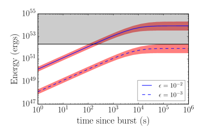
Figure 1 illustrates, for a post-merger remnant inferred from GRB140903A with a fiducial , an ellipticity violates the energy-budget constraint. Based on these energy considerations the upper limit on ellipticity for GRB140903A is . In reality, the moment of inertia for a long-lived post-merger remnant is likely higher than the fiducial value we use here, however all our limits can be scaled appropriately for different values of . In particular, the moment of inertia is inversely proportional to the inferred upper limit on ellipticity, because the rotational energy grows linearly with , but the gravitational-wave energy grows quadratically. Our fiducial moment of inertia therefore provides a conservative limit on the ellipticity.
II.2 Optimal matched filter statistic
The matched-filter signal-to-noise ratio is given by Cutler1994
| (12) |
where is the combination of signal and noise , is the template, and denotes the noise-weighted inner product (Cutler1994), defined by
| (13) |
Here denotes the Fourier transform of , its complex conjugate, and is the noise power spectral density. The optimal matched-filter signal-to-noise ratio is achieved when the template matches the data precisely:
| (14) |
In this analysis, the threshold signal-to-noise ratio required to make a detection is , which is derived in Sec. IV. In Fig. 2 we show the region of parameter space where we could detect a signal from a post-merger remnant at the same distance as GW170817 ( Mpc). We assume , (top panel) and (bottom panel), and Hz. We use these values of and as they are the maximum likelihood parameters from GRB140903A using the method detailed in Sec. III.
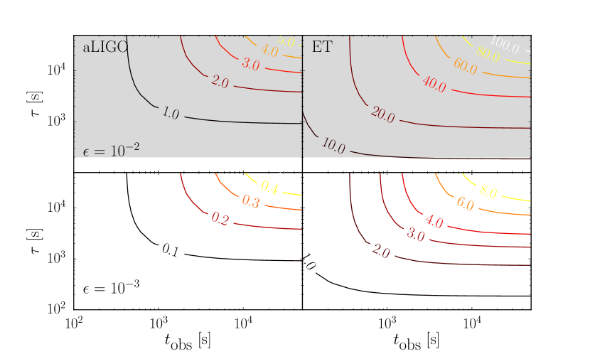 |
The left-hand side of Fig. 2 shows it is theoretically possible for gravitational waves from such an object to be observable by aLIGO operating at design sensitivity observing_aligo if s and s. The right-hand side shows that the Einstein Telescope (ET), a proposed third generation detector ET, can detect such a signal if s and s for . We note that GRB140903A has s. However, as shown in Sec. II.1 this large ellipticity is nonphysical for GRB140903A-like post-merger remnant in all of the parameter space required to detect a signal with aLIGO. A physically realistic ellipticity rules out any prospect of detection with aLIGO for a GRB140903A-like post-merger signal at Mpc and requires s and s for detecting the same signal with ET.
The optimal matched filter signal-to-noise ratio (Eq. 14) can also be used to estimate the distance out to which we can detect a signal.
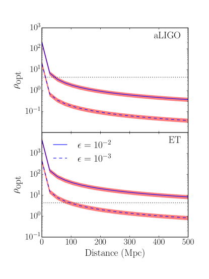
Figure 3 shows that with aLIGO at design sensitivity the furthest distance we can detect a signal with maximum likelihood parameters inferred from GRB140903A is and Mpc for and respectively, while with ET the distances are Mpc and Mpc respectively. As we showed in Sec. II.1, for the parameters inferred from GRB140903A only an ellipticity is physical, post-merger remnants with longer spin-down timescale, , can be detected to larger distances assuming that is physical for those parameters.
The optimal matched filter is the maximum signal-to-noise ratio one can achieve in a matched filter search. In practice, this limit is unobtainable with current computational resources. As shown by Fig. 2 and Fig. 3, to achieve and make a detection of gravitational waves, we need to observe a signal for at least seconds with aLIGO at design sensitivity. At large observation times, the volume of parameter space imposed by uniform priors becomes unfeasible for a realistic gravitational-wave search (see Sec. IV). In the following section, we demonstrate how to constrain the priors, and hence the search parameter space, using X-ray observations of SGRBs
III X-ray afterglow
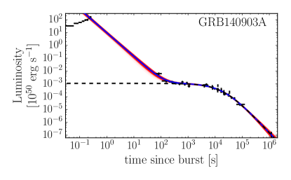
Short gamma-ray bursts are often followed by X-ray emission lasting up to many tens of thousands of seconds Rowlinson2010; Rowlinson2013; LaskyLeris2017; Lu2015. Such an X-ray afterglow was not observed for GRB170817A. In Fig. 4 we show the X-ray afterglow of GRB140903A with data from the Neil Gehrels Swift and Chandra satellites (Troja2016).
Rowlinson2013 modelled the X-ray afterglows of several SGRBs with two components. Firstly, an initial power-law decay,
| (15) |
where is the luminosity, is the power-law amplitude, and is the power-law exponent. Here, the decay exponent can be fixed to , where is the photon index of the prompt emission, or allowed to vary. The second component is a luminosity law to model the energy injection from a millisecond magnetar that is spinning down through magnetic dipole radiation () Zhang2001; Dai1998. LaskyLeris2017 extended this model to include other forms of radiation causing spin-down, which is derived by utilising the general torque equation (Eq. 1). The luminosity of the second component therefore comes directly from the nascent neutron star, and can be expressed as
| (16) |
where, is the initial luminosity at the onset of the plateau phase and is related to the initial gravitational-wave frequency by
| (17) |
where encodes the efficiency of converting spin-down energy to X-rays. Our numerical model involves fitting Eq. (15) and (16) to the X-ray observations from Swift and Chandra. However, instead of fitting we fit our initial gravitational-wave frequency . We use a Markov Chain Monte Carlo algorithm Foreman-Mackey2013 to fit the X-ray afterglow of SGRBs with our model using uniform priors for , , , , and between [, ], [, ], [, ], [, ], and [, ] respectively. Fits we have made to GRB140903A are shown in Fig. 4. We determine the posterior distribution on our parameters , , and which are shown in Fig. 5. In the following section, we discuss how these posteriors can be used as priors for a targeted search for the post-merger remnant associated with an SGRB.
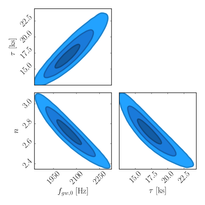
IV Gravitational-wave search pipeline
Here we describe a pipeline to search for gravitational waves from a spinning down millisecond magnetar. The algorithm can be summarised as follows:
-
1.
Generate posterior distributions on the three waveform parameters , and using the X-ray afterglow observations of a specific SGRB as described in Sec. III.
-
2.
These posterior distributions, along with uniform priors on and , serve as priors for our waveform model. Template waveforms are generated from points in these priors.
-
3.
Templates are used to calculate the matched filter signal-to-noise ratio using LIGO data at the time of the SGRB.
The same pipeline can also be adopted with unconstrained uniform priors in step 1, in the case where no X-ray data is available. However, the number of templates required for a matched-filter search becomes computationally unfeasible. We quantify this throughout this section.
We calculate the fitting factor Apostolatos1995, also commonly referred to as the overlap (e.g., Cornish2012). The fitting factor is the penalty in signal-to-noise ratio one suffers due to comparing templates that do not precisely match the signal: . We want to minimize this penalty while maximizing the signal-to-noise ratio.
To calculate the we randomly draw one value of each parameter from our priors and construct a model waveform using the waveform model described in Sec II. We assume this is our true template, . We determine the optimal matched filter signal-to-noise ratio for this template using Eq. (14), We randomly draw from our priors excluding our ‘true template’ and create a random template, , where i labels the drawn sample. We compute the matched filter signal-to-noise ratio (Eq. 12), . We calculate for N random templates. In the limit of infinite templates, .
The maximum fitting factor is defined as
| (18) |
where is the maximum matched-filter signal-to-noise ratio from a population of N templates. In the limit of an infinite number of templates, , assuming our signal parameters are within our template parameter space. Creating a large number of templates is computationally expensive. We therefore want to minimise the number of templates we need. Additionally, we want to maximise our signal-to-noise ratio by creating templates for a longer duration.