A generalized spatial sign
covariance matrix

Abstract

The well-known spatial sign covariance matrix (SSCM) carries out a radial transform which moves all data points to a sphere, followed by computing the classical covariance matrix of the transformed data. Its popularity stems from its robustness to outliers, fast computation, and applications to correlation and principal component analysis. In this paper we study more general radial functions. It is shown that the eigenvectors of the generalized SSCM are still consistent and the ranks of the eigenvalues are preserved. The influence function of the resulting scatter matrix is derived, and it is shown that its breakdown value is as high as that of the original SSCM. A simulation study indicates that the best results are obtained when the inner half of the data points are not transformed and points lying far away are moved to the center.

Keywords: multivariate statistics, orthogonal equivariance, outliers, radial transform,
robust location and scatter.

1 Introduction

Robust estimation of the covariance (scatter) matrix is an important and challenging problem. Over the last decades, many robust estimators for the covariance matrix have been developed. Many of them possess the attractive property of affine equivariance, meaning that when the data are subjected to an affine transformation the estimator will transform

accordingly. However, all highly robust affine equivariant scatter estimators have a combinatorial time complexity. Other estimators posses the less restrictive property of orthogonal equivariance. This means that the estimators commute with orthogonal transformations, which are characterized by orthogonal matrices and include rotations and reflections.

The most well-known orthogonally equivariant scatter estimator is the spatial sign covariance matrix (SSCM) proposed independently by Marden (1999) and Visuri et al. (2000) and studied in more detail by Magyar and Tyler (2014) and Dürre et al. (2014, 2016) among others. The estimator computes the regular covariance matrix on the spatial signs of the data, which are the projections of the location-centered datapoints on the unit sphere. Somewhat surprisingly, this transformation yields a consistent estimator of the eigenvectors of the true covariance matrix (Marden, 1999) under relatively general conditions on the underlying distribution. Of course the eigenvalues are different from the eigenvalues of the true covariance matrix, but Visuri et al. (2000) have shown that the order of the eigenvalues is preserved. We build on this idea by illustrating that the SSCM is part of a larger class of orthogonally equivariant estimators, all of which estimate the eigenvectors of the true covariance matrix and preserve the order of the eigenvalues.

The SSCM is easy to compute, and has been used extensively in several applications. The most common use of the SSCM is probably in the context of (functional) spherical PCA as developed by Locantore et al. (1999), Visuri et al. (2001), Croux et al. (2002) and Taskinen et al. (2012). Like classical PCA, spherical PCA aims to find a lower dimensional subspace that captures most of the variability in the data. After centering the data, spherical PCA projects the data onto the unit (hyper)sphere before searching for the directions of highest variability. This projection gives all data points the same weight in the estimation of the subspace, thereby limiting the influence of potential outliers. The directions (‘loadings’) of spherical PCA thus correspond to the eigenvectors of the SSCM scatter matrix. The corresponding scores are usually taken to be the inner products of the loading vectors with the original (centered) data points, not with the projections of the data points on the sphere. Some concrete applications of spherical PCA are about the shape of the cornea in ophthalmology as analyzed by Locantore et al. (1999), and for multichannel signal processing as illustrated in Visuri et al. (2000).

In addition to spherical PCA, there also has been a lot of recent research on the use of the SSCM for constructing robust correlation estimators (Dürre et al., 2015; Dürre and Vogel, 2016; Dürre et al., 2017). The main focus of this work is on results including asymptotic properties, the eigenvalues, and the influence function which measures robustness. A third application of the SSCM is its use as an initial estimate for more involved robust scatter estimators (Croux et al., 2010; Hubert et al., 2012). The SSCM is particularly well-suited for this task as it is very fast and highly robust against outlying observations and therefore often yields a reliable starting value. Another application of the SSCM is to testing for sphericity (Sirkia et al., 2009), which uses the asymptotic properties of the SSCM in order to assess whether the underlying distribution of the data deviates substantially from a spherical distribution. Serneels et al. (2006) use the spatial sign transform as an initial preprocessing step in order to obtain a robust version of partial least squares regression. Finally, Boente et al. (2018) study SCCM as an operator for functional data analysis.

The next section introduces a generalization of the SSCM and studies its properties. Section 3 compares the performance of several members of this class in a small simulation study, and Section 5 concludes. All proofs can be found in the Appendix.

2 Methodology

2.1 Definition

Definition 1.

Let $X$ be a $p$-variate random variable and $\mu$ a vector serving as its center. Define the generalized spatial sign covariance matrix (GSSCM) of $X$ by

$$S_{g_{X}}(X)=E_{F_{X}}[g_{X}(X-\mu)g_{X}(X-\mu)^{T}]\;,$$ (1)

where the function $g_{X}$ is of the form

$$g_{X}(t)=t\;\xi_{X}(||t||)\;,$$ (2)

where we call $\xi_{X}:\mathbb{R}^{+}\to\mathbb{R}^{+}$ the radial function and $||\cdot||$ is the Euclidean norm.

Note that the form of $g_{X}$ in (2) precisely characterizes an orthogonally equivariant data transformation as shown by Hampel et al. (1986), p. 276. Also note that the regular covariance matrix corresponds to $\xi_{X}(r)=1$, and that $\xi_{X}(r)=1/r$ yields the SSCM.

For a finite data set $\bm{X}=\{x_{1},\ldots,x_{n}\}$ the GSSCM is given by

$$S_{g_{\bm{X}}}(\bm{X})=\frac{1}{n}\sum_{i=1}^{n}{\xi^{2}_{\bm{X}}(||x_{i}-T(\bm{X})||)(x_{i}-T(\bm{X}))(x_{i}-T(\bm{X}))^{T}}$$ (3)

where $T$ is a location estimator. Note that the SSCM gives the $x_{i}$ with $||x_{i}-T(\bm{X})||<1$ a weight higher than 1, but in general this is not required. In fact, the other functions we will propose satisfy $\xi_{\bm{X}}(r)\leqslant 1$ for all $r$.

In the above definitions, we added the subscript $X$ or $\bm{X}$ to the functions $g$ and $\xi$ to indicate that they can depend on $X$ or $\bm{X}$. In what follows we will drop these subscripts to ease the notational burden. We will study the following functions $\xi$:

1. Winsorizing (Winsor):

   $$\xi(r)=\begin{cases}1&\mbox{ if }r\leqslant Q_{2}\\ Q_{2}/r&\mbox{ if }Q_{2}<r\;.\\ \end{cases}$$ (4)

2. Quadratic Winsor (Quad):

   $$\xi(r)=\begin{cases}1&\mbox{ if }r\leqslant Q_{2}\\ Q_{2}^{2}/r^{2}&\mbox{ if }Q_{2}<r\;.\\ \end{cases}$$ (5)

3. Ball:

   $$\xi(r)=\begin{cases}1&\mbox{ if }r\leqslant Q_{2}\\ 0&\mbox{ if }Q_{2}<r\;.\end{cases}$$ (6)

4. Shell:

   $$\xi(r)=\begin{cases}0&\mbox{ if }r<Q_{1}\\ 1&\mbox{ if }Q_{1}\leqslant r\leqslant Q_{3}\\ 0&\mbox{ if }Q_{3}<r\;.\end{cases}$$ (7)

5. Linearly Redescending (LR):

   $$\xi(r)=\begin{cases}1&\mbox{ if }r\leqslant Q_{2}\\ (Q_{3}^{*}-r)/(Q_{3}^{*}-Q_{2})&\mbox{ if }Q_{2}<r\leqslant Q_{3}^{*}\\ 0&\mbox{ if }Q_{3}^{*}<r\;.\end{cases}$$ (8)

The cutoffs $Q_{1}$, $Q_{2}$, $Q_{3}$ and $Q_{3}^{*}$ depend on the Euclidean distances $||x_{i}-T(\bm{X})||$ by

$$Q_{1} =\left(\mbox{hmed}_{i}(||x_{i}-T(\bm{X})||^{\frac{2}{3}})-\mbox{hmad}_{i}(||x_{i}-T(\bm{X})||^{\frac{2}{3}})\right)^{\frac{3}{2}}$$

$$Q_{2} =\left(\mbox{hmed}_{i}(||x_{i}-T(\bm{X})||^{\frac{2}{3}})\right)^{\frac{3}{2}}=\mbox{hmed}_{i}(||x_{i}-T(\bm{X})||)$$

$$Q_{3} =\left(\mbox{hmed}_{i}(||x_{i}-T(\bm{X})||^{\frac{2}{3}})+\mbox{hmad}_{i}(||x_{i}-T(\bm{X})||^{\frac{2}{3}})\right)^{\frac{3}{2}}$$

$$Q_{3}^{*} =\left(\mbox{hmed}_{i}(||x_{i}-T(\bm{X})||^{\frac{2}{3}})+1.4826\;\mbox{hmad}_{i}(||x_{i}-T(\bm{X})||^{\frac{2}{3}})\right)^{\frac{3}{2}},$$

where hmed and hmad are variations on the median and median absolute deviation given by the order statistic $\mbox{hmed}(y_{1},\ldots,y_{n})=y_{(h)}$ and $\mbox{hmad}(y_{1},\ldots,y_{n})=\mbox{hmed}_{i}|y_{i}-hmed_{j}(y_{j})|$ where $h=\left\lfloor\frac{n+p+1}{2}\right\rfloor$ . The $\frac{2}{3}$ power in these formulas is the Wilson-Hilferty transformation (Wilson and Hilferty, 1931) to near normality. In Section A.1 of the Appendix it is verified that this transformation brings the above cutoffs close to the theoretical ones, which are quantiles of a convolution of Gamma random variables with different scale parameters.

Figure 1 shows the above functions $\xi$ and that of the SSCM for distances whose square follows the $\chi_{2}^{2}$ distribution. The $\xi$ of the SSCM is the only one which upweights observations close to the center. The Winsor $\xi$ and its square have a similar shape, but the latter goes down faster. The Ball and Shell $\xi$ functions are both designed to give a weight of 1 to half (in fact, $h$) of the data points and 0 to the remainder, to make them comparable. Ball does this by giving a weight of 1 to the $h$ points with the smallest distances. Shell is inspired by the idea of Rocke to both downweight observations with very high and very low distances from the center (Rocke, 1996). The Linearly Redescending $\xi$ is a compromise between the Ball and the Quad $\xi$ functions.

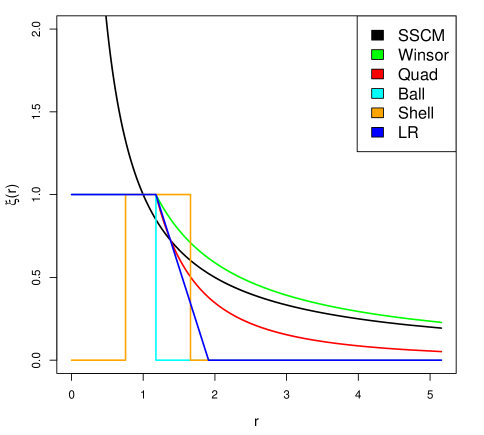
Figure 1: Radial functions $\xi$

2.2 Preservation of the eigenstructure

In what follows, we assume that the distribution $F_{X}$ of $X$ has an elliptical density with center zero and that its covariance matrix $\Sigma=E_{F_{X}}[XX^{T}]$ exists. Therefore, $X$ can be written as $X=UDZ$ where $U$ is a $p\times p$ orthogonal matrix, $D$ is a $p\times p$ diagonal matrix with strictly positive diagonal elements, and $Z$ is a $p$-variate random variable which is spherically symmetric, i.e. its density is of the form $f_{Z}(z)\sim w(||z||)$ where $w$ is a decreasing function. Assume w.l.o.g. that the covariance matrix of $Z$ is $I_{p}$. The following proposition says that $S_{g}(X)$ has the same eigenvectors as $\Sigma$ and preserves the ranks of the eigenvalues.

Proposition 1.

Let $X=UDZ$ be a $p$-variate random variable as described above, with $D=\mbox{diag}(\delta_{1},\ldots,\delta_{p})$ where $\delta_{1}\geqslant\ldots\geqslant\delta_{p}>0$. Assume that the covariance matrix $S_{g}=E_{F_{X}}[g(X)g(X)^{T}]$ of $g(X)$ exists. Then $\Sigma$ and $S_{g}$ can be diagonalized as

$$\Sigma=U\Lambda U^{T}\;\;\;\mbox{ and }\;\;\;S_{g}=U\Lambda_{g}U^{T}$$

where $\Lambda=\mbox{diag}(\lambda_{1},\ldots,\lambda_{p})$ with $\lambda_{j}=\delta_{j}^{2}$ and $\Lambda_{g}=\mbox{diag}(\lambda_{g,1},\ldots,\lambda_{g,p})$ with $\lambda_{g,1}\geqslant\ldots\geqslant\lambda_{g,p}>0$ and $\lambda_{j}=\lambda_{j+1}\Leftrightarrow\lambda_{g,j}=\lambda_{g,j+1}$ .

This proposition justifies the generalized SSCM approach.

2.3 Location estimator

So far we have not specified any location estimator $T$. For the SSCM the most often used location estimator is the spatial median, see e.g. Gower (1974) and Brown (1983), which we denote by $T_{0}$. The spatial median of a dataset $\bm{X}=\{x_{1},\ldots,x_{n}\}$ is defined as

$$T_{0}(\bm{X})=\operatorname*{arg\,min}_{\theta}{\sum_{i=1}^{n}{||x_{i}-\theta||}}\;.$$

In order to improve its robustness against a substantial fraction of outliers we propose to use the k-step least trimmed squares (LTS) estimator. The LTS method was originally proposed in regression (Rousseeuw, 1984), and for multivariate location it becomes

$$T_{\mbox{LTS}}(\bm{X})=\operatorname*{arg\,min}_{\theta}{\sum_{i=1}^{h}||x_{\bullet}-\theta||^{2}_{(i)}}$$

where the subscript $(i)$ stands for the i-th smallest squared distance. (Without the square this becomes the least trimmed absolute distance estimator studied in Chatzinakos et al. (2016).) For the multivariate location LTS the C-step of (Rousseeuw and Van Driessen, 1999) simplifies to

Definition 2.

(C-step) Fix $h=\left\lfloor(n+1)/2\right\rfloor$. Given a location estimate $T_{j-1}(\bm{X})$ we take the set $I_{j}=\{i_{1},\ldots,i_{h}\}\subset\{1,\ldots,n\}$ such that $\{||x_{i}-T_{j-1}(\bm{X})||;\;i\in I_{j}\}$ are the $h$ smallest distances in the set $\{||x_{i}-T_{j-1}(\bm{X})||;\;i=1,\ldots,n\}$. The C-step then yields

$$T_{j}(\bm{X})=\frac{1}{h}\sum_{i\in I_{j-1}}x_{i}\;.$$

The C-step is fast to compute, and guaranteed to lower the LTS objective. The k-step LTS is then the result of $k$ successive C-steps starting from the spatial median $T_{0}(\bm{X})$ .

It is also possible to avoid the estimation of location altogether, by calculating the GSSCM on the $O(n^{2})$ pairwise differences of the data points. This approach is called the “symmetrization” of an estimator, but is more computationally intensive. Visuri et al. (2000) studied the symmetrized SSCM and called it Kendall’s $\tau$ covariance matrix.

2.4 Robustness properties

A major reason for the SSCM’s popularity is its robustness against outliers. Robustness can be quantified by the influence function and the breakdown value. We will study both for the GSSCM.

The influence function (Hampel et al. (1986)) quantifies the effect of a small amount of contamination on a statistical functional $T$. Consider the contaminated distribution $F_{\varepsilon,z}=(1-\varepsilon)F+\varepsilon\Delta(z)$, where $\Delta(z)$ is the distribution that puts all its mass in $z$. The influence function of $T$ at $F$ is then given by

$$\mbox{IF}(z,T,F)=\lim_{\varepsilon\to 0}\frac{T(F_{\varepsilon,z})-T(F)}{\varepsilon}=\frac{\partial}{\partial\varepsilon}\;T(F_{\varepsilon,z})\bigg{|}_{\varepsilon=0}.$$

For the generalized SSCM class we obtain the following result:

Proposition 2.

Denote $S_{g}(F)=\Xi_{g}$ and let $\mu=0$ in (1). The influence function of $S_{g}$ at the distribution $F$ is given by:

$$\mbox{IF}(z,S_{g},F)=\left.\frac{\partial}{\partial\varepsilon}S(F_{\varepsilon,z})\right|_{\varepsilon=0}=g(z)g(z)^{T}-\Xi_{g}+\left.\frac{\partial}{\partial\varepsilon}\int{g_{\varepsilon}(X)g_{\varepsilon}(X)^{T}dF(X)}\right|_{\varepsilon=0}\;.$$ (9)

If $g$ does not depend on $F$, the last term of (9) vanishes. For example, for $g(t)=t$, we retrieve the IF of the classical covariance matrix $\mbox{IF}(z,\Sigma,F)=zz^{T}-\Sigma$ , and for $g(t)=t/||t||$ we obtain $\mbox{IF}(z,\mbox{SSCM},F)=\left(\frac{z}{||z||}\right)\left(\frac{z}{||z||}\right)^{T}-\mbox{SSCM}(F)$ in line with the findings of Croux et al. (2002). For the GSSCM estimators defined by the functions (4)–(8) the last term of (9) remains, and the expressions of their IF can be found in Section A.3 of the Appendix.

In order to visualize the influence function we consider the bivariate standard normal case, i.e. $F=N(0,I_{2})$. We put contamination at $(z,z)$ or $(z,0)$ for different values of $z$ and plot the IF for the diagonal elements and the off-diagonal element. Note that we cannot compare the raw IFs directly as $S_{g}(F)=\Xi_{g}=c_{g}I$ where $c_{g}=\int{g_{1}(X)^{2}dF(X)}$ hence $\Xi_{g}$ is only equal to $I_{2}$ up to a factor. In order to make the estimators consistent for this distribution we can divide them by $c_{g}$ , and so we plot $\mbox{IF}(z,S_{g},F)/c_{g}$ in Figure 2.

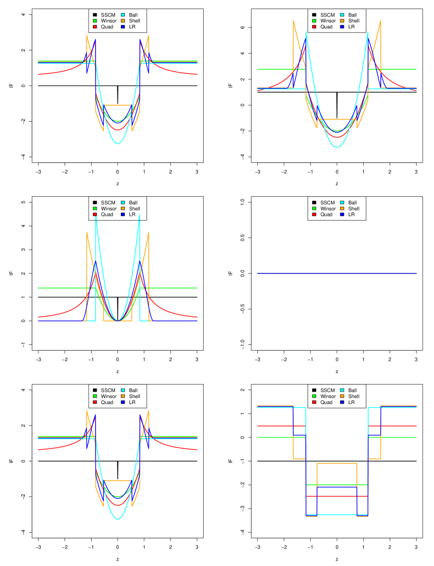
Figure 2: Influence functions of the GSSCM at the bivariate standard normal distribution for contamination at $(z,z)$ (left) and $(z,0)$ (right). The rows correspond to the first diagonal element $S_{11}$ (top), the off-diagonal element $S_{12}$ (middle), and $S_{22}$ (bottom).

The rows in Figure 2 correspond to the IF of the first diagonal element $S_{11}$ (top), the off-diagonal element $S_{12}$ (middle) and the element $S_{22}$ (bottom). Let’s first consider the left part of the figure, which contains the IFs for an outlier in $(z,z)$. By symmetry, the IFs of the diagonal elements $S_{11}$ and $S_{22}$ are the same here. In the regions where the function $\xi$ is 1 the IF is quadratic, like that of the classical covariance. The diagonal elements of the IF of the SSCM are zero, except at $z=0$ where it takes the value $-1$. The Quad IF is the only one which redescends as $|z|$ increases, whereas the others are also bounded but stabilize at a value around $1.3$. The shape of the IF of the Ball estimator resembles that of the univariate Huber M-estimator of scale.

For the IF of the off-diagonal element $S_{12}$ the picture is very different. All are redescending except for the SSCM and Winsor. Here it is Winsor whose IF resembles that of Huber’s M-estimator of scale. Note that the IFs of the Ball and Shell estimators have large jumps at their cutoff values. The discontinuities in the IFs are due to the fact that the cutoffs depend on the median and the MAD of the distances $||X||^{2/3}$, as both the median and the MAD have jumps in their IF.

The right panel of Figure 2 shows the influence functions for an outlier in $(z,0)$. In this case the IFs of the diagonal elements $S_{11}$ and $S_{22}$ are no longer the same, as the symmetry is broken. The IFs of $S_{11}$ are again quadratic where $\xi=1$, with jumps at the cutoffs. Note that these cutoffs are now located at different values of $z$, as $||(z,0)||\neq||(z,z)||$. The IF of the off-diagonal element is constant at 0, indicating that $S_{12}$ remains zero even when there is an outlier at $(z,0)$. Finally, for the second diagonal element $S_{22}$ the IF of the SSCM is $-1$. This is because adding $\varepsilon$ of contamination at $(z,0)$ reduces the mass of the remaining part of $F$ by $\varepsilon$ which lowers the estimated scatter in the vertical direction. For the other estimators there is an additional effect of $(z,0)$ on the cutoffs, which causes the discontinuities.

A second tool for quantifying the robustness of an estimator is the finite-sample breakdown value (Donoho and Huber, 1983). For a multivariate location estimator $T$ and a dataset $\bm{X}$ of size $n$, the breakdown value is the smallest fraction of the data that needs to be replaced by contamination to make the resulting location estimate lie arbitrarily far away from the original location $T(\bm{X})$. More precisely:

$$\varepsilon^{*}(T,\bm{X})=\min{\left\{\frac{m}{n}:\sup_{\bm{X}_{m}^{*}}{||T(\bm{X})-T(\bm{X}^{*})||}=\infty\right\}}$$

where $\bm{X}_{m}^{*}$ ranges over all datasets obtained by replacing any $m$ points of $\bm{X}$ by arbitrary points.

For a multivariate estimator of scale $S$, the breakdown value is defined as the smallest fraction of contamination needed to make an eigenvalue of $S$ either arbitrarily large or arbitrarily close to zero. We denote the eigenvalues of $S(\bm{X})$ by $\lambda_{1}(S(\bm{X}))\geqslant\ldots\geqslant\lambda_{p}(S(\bm{X}))$. The breakdown value of $S$ is then given by:

$$\varepsilon^{*}(S,\bm{X})=\min{\left\{\frac{m}{n}:\sup_{\bm{X}_{m}^{*}}{\max{\{\lambda_{1}(S(\bm{X}_{m}^{*})),\lambda_{p}(S(\bm{X}_{m}^{*}))^{-1}\}}=\infty}\right\}}\;.$$

For the results on breakdown we assume the following conditions on the function $\xi$:

1. The function $\xi$ takes values in $[0,1]$.

2. For any dataset $\bm{X}$ it holds that $\#\{x_{i}|\;\xi(||x_{i}-T(\bm{X})||)=1\}\geqslant\left\lfloor\frac{n+p+1}{2}\right\rfloor$.

3. For any vector $t$ it holds that $||g(t)||=||t||\xi(||t||)\leqslant\mbox{hmed}_{i}(d_{i})+1.4826\,\mbox{hmad}_{i}(d_{i})$ .

Note that all functions $\xi$ proposed in (4)–(8) satisfy these assumptions. The following proposition gives the breakdown value of the GSSCM scatter estimator $S_{g}$.

Proposition 3.

Let $\bm{X}=\{x_{1},\ldots,x_{n}\}$ be a $p$-dimensional dataset in general position, meaning that no $p+1$ points lie on the same hyperplane. Also assume that the location estimator $T$ has a breakdown value of at least $\left\lfloor(n-p+1)/2\right\rfloor/n$ . Then

$$\epsilon^{*}\left(S_{g},\bm{X}\right)=\frac{\left\lfloor(n-p+1)/2\right\rfloor}{n}\;.$$

As we would like the GSSCM scatter estimator to attain this breakdown value, we have to use a location estimator whose breakdown value is at least $\left\lfloor(n-p+1)/2\right\rfloor/n$ . The following proposition verifies that the k-step LTS estimator satisfies this, and even attains the best possible breakdown value for translation equivariant location estimators.

Proposition 4.

The k-step LTS estimator $T_{k}$ satisfies

$$\varepsilon^{*}(T_{k},\bm{X})=\frac{\left\lfloor(n+1)/2\right\rfloor}{n}$$

at any p-variate dataset $\bm{X}=\{x_{1},\ldots,x_{n}\}$. When the C-steps are iterated until convergence $(k\to\infty)$, the breakdown value remains the same.

3 Simulation study

We now perform a simulation study comparing the GSSCM versions (4)–(8). As the estimators are orthogonally equivariant, it suffices to generate diagonal covariance matrices. We generate $m=1000$ samples of size $n=100$ from the multivariate Gaussian distribution of dimension $p=10$ with center $\mu=\bm{0}$ and covariance matrices $\Sigma_{1}=I_{p}$ (‘constant eigenvalues’), $\Sigma_{2}=\mbox{diag}(10,9,\ldots,1)$ (‘linear eigenvalues’), and $\Sigma_{3}=\mbox{diag}(10^{2},9^{2},\ldots,1)$ (‘quadratic eigenvalues’). To assess robustness we also add 20% and 40% of contamination in the direction of the last eigenvector, at the point $(0,\ldots,0,\gamma)$ for several values of $\gamma$. For the location estimator $T$ in (3) we used the k-step LTS with $k=5$.

For measuring how much the estimated $\widehat{\Sigma}$ deviates from the true $\Sigma$ we use the Kullback-Leibler divergence (KLdiv) given by

$$\mbox{KLdiv}(\widehat{\Sigma},\Sigma)=\mbox{trace}(\widehat{\Sigma}\Sigma^{-1})-\log(\det(\widehat{\Sigma}\Sigma^{-1}))-p\;.$$

We also consider the shape matrices $\widehat{\Gamma}=(\mbox{det}\widehat{\Sigma})^{-1/p}\widehat{\Sigma}$ and $\Gamma=(\mbox{det}\Sigma)^{-1/p}\Sigma$ which have determinant 1, and compute $\mbox{KLdivshape}(\widehat{\Sigma},\Sigma):=\mbox{KLdiv}(\widehat{\Gamma},\Gamma)$ . Both the KLdiv and the KLdivshape are then averaged over the $m=1000$ replications.

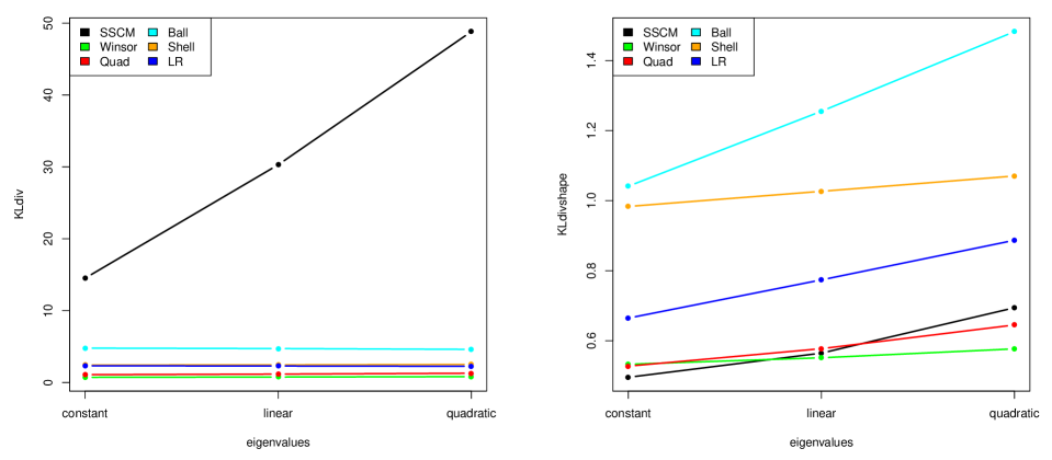
Figure 3: Simulation results: KLdiv (left) and KLdivshape (right) for the uncontaminated normal distribution, with constant, linear and quadratic eigenvalues.

Figure 3 shows the simulation results on the uncontaminated data. Looking at KLdiv (left panel) we note that the SSCM deviates the most from the true covariance matrix $\Sigma$. Among the other choices, Winsor and Quad have the lowest bias, followed by LR, Shell, and Ball. When looking only at the shape component (right panel), SSCM performs the best when the distribution is spherical (constant eigenvalues), in line with Remark 3.1 in (Magyar and Tyler, 2014). However, it loses this dominant performance once the distribution deviates from sphericity. Among the other GSSCM methods Winsor performs the best, followed by its quadratic counterpart, LR, Shell, and finally Ball.

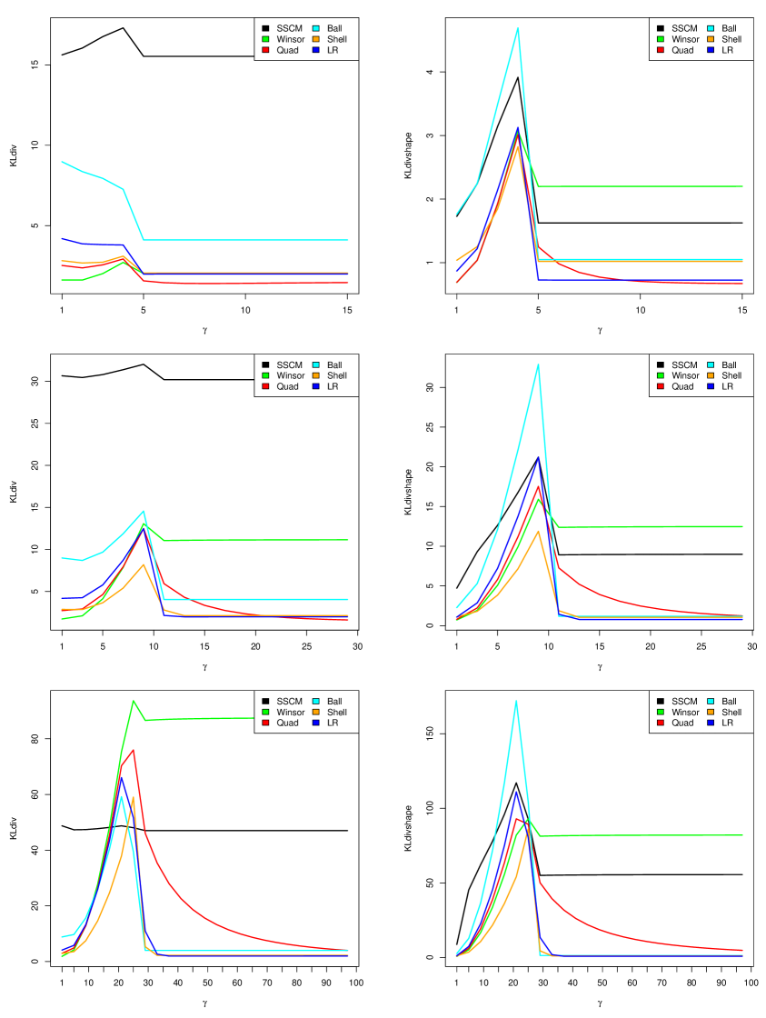
Figure 4: Simulation results: KLdiv (left) and KLdivshape (right) for the normal distribution with constant (top), linear (middle) and quadratic (bottom) eigenvalues and 20% of contamination. The outliers were placed at the point $(0,\ldots,0,\gamma)$.

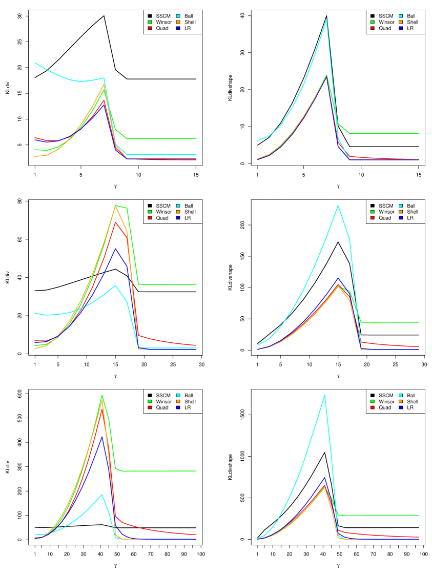
Figure 5: Simulation results: KLdiv (left) and KLdivshape (right) for the normal distribution with constant (top), linear (middle) and quadratic (bottom) eigenvalues and 40% of point contamination.

The result for the simulation with 20% of point contamination is presented in Figure 4. All plots are as a function of $\gamma$, which indicates the position of the outliers. In the left panel (KLdiv) the SSCM has a large bias. The Winsor GSSCM, which did very well in the uncontaminated setting, now has a disappointing performance when the eigenstructure becomes more challenging with linear or quadratic eigenvalues. Quad performs a lot better, but also suffers under quadratic eigenvalues. LR and Shell perform the best here, followed by Ball. Their redescending nature helps them for far outliers. The conclusions for the shape component (right panel) are largely similar, except that Winsor and especially Ball look worse here.

The simulation results for 40% of contamination are shown in Figure 5. The KLdiv plots on the left indicate that the SSCM performs poorly for constant and linear eigenvalues, and looks better for quadratic eigenvalues but not when $\gamma$ is large (far outliers). Winsor performs badly for linear and quadratic eigenvalues, whereas Quad does much better. Ball looks okay except for relatively small $\gamma$. LR and Shell perform the best for both small and large $\gamma$, and are okay for intermediate $\gamma$. When estimating the shape component (right panels) SSCM and Winsor have the worst performance overall, whereas Ball also does poorly for small to intermediate $\gamma$. LR and Shell are the best picks here. Quad does almost as well, but redescends more slowly.

4 Application: principal component analysis

We analyze a multivariate dataset from a study by Reaven and Miller (1979). The dataset contains 5 numerical variables for 109 subjects, consisting of 33 overt diabetes patients and 76 healthy people. The variables are body weight, fasting plasma glucose, area under the plasma glucose curve, area under the plasma insulin curve, and steady state plasma glucose response. These data were previously analyzed by Mozharovskyi et al. (2015) in the context of clustering using statistical data depth, and is available in the R package ddalpha (Pokotylo et al., 2016) under the tag chemdiab_2vs3. Here we analyze the data by principal component analysis. We first standardize the data, as the variables have quite different scales. Denote the standardized observations by $z_{i}$ for $i\in\{1,\ldots,109\}$.

We consider the diabetes patients as outliers and would like the PCA subspace to model the variability within the healthy patients. For classical PCA, the PCA subspace corresponds to the linear span of the $k$ eigenvectors (also called ‘loadings’) of the covariance matrix which correspond with the $k$ largest eigenvalues. In similar fashion we can perform PCA based on the GSSCM, by considering the linear span of its $k$ first eigenvectors. We take $k=3$ components, thereby explaining more than 95 % of the variance.

Figure 6 shows the scores with respect to the first 3 loadings for classical PCA and GSSCM PCA. The scores $s_{i}$ are the projections of the observations $z_{i}$ onto the PCA subspace, i.e. $s_{i,j}=z_{i}^{T}v_{j}$ where $v_{j}$ denotes the $j$-th eigenvector. From these plots, it is clear that the first eigenvector of the classical PCA is heavily attracted by the diabetes patients. As a result, the outliers are only distinguishable in their scores with respect to the first principal component. This is very different for the GSSCM PCA, where the principal components seem to fit the healthy patients better, resulting in outlying scores for the diabetes patients with respect to several principal components.

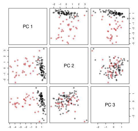
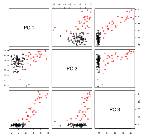
Figure 6: Scores from the 3 first loading vectors of classical PCA (left) and GSSCM PCA (right).

In addition to the scores plots, the PCA outlier map of Hubert et al. (2005) can serve as a diagnostic tool for identifying outliers. It plots the orthogonal distance $\mbox{OD}_{i}$ against the score distance $\mbox{SD}_{i}$ for every observation $z_{i}$ in the dataset. The score distance of observation $i$ captures the distance between the observation and the center of the data within the PCA subspace. It is given by $\mbox{SD}_{i}=\sqrt{\sum_{j=1}^{3}{(s_{ij}/\hat{\sigma}_{j}})^{2}}$ where $\hat{\sigma}_{j}$ denotes the scale of the $j$-th scores. For classical PCA $\hat{\sigma}_{j}$ is their standard deviation, whereas for GSSCM PCA we take their median absolute deviation. The orthogonal distance to the PCA subspace is given by $\mbox{OD}_{i}=||z_{i}-Vs_{i}||$ where $V$ is the $5\times 3$ matrix containing the 3 eigenvectors in its columns. Both the score distances and the orthogonal distances have cutoffs, described in Hubert et al. (2005). Figure 7 shows the outlier maps resulting from the classical PCA and the GSSCM PCA. Classical PCA clearly fails to distinguish the diabetes patients from the healthy subjects. In contrast, GSSCM PCA flags most of the diabetes patients as having both an abnormally high orthogonal distance to the PCA subspace as well as having a projection in the PCA subspace far away from those of the healthy subjects.

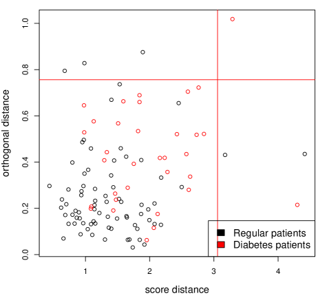
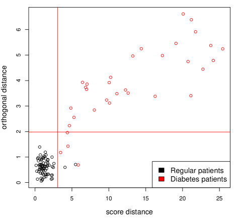
Figure 7: Outlier maps based on classical PCA (left) and GSSCM PCA (right).

5 Conclusions

The spatial sign covariance matrix (SSCM) can be seen as a member of a larger class called Generalized SSCM (GSSCM) estimators in which other radial functions are allowed. It turns out that the GSSCM estimators are still consistent for the true eigenvectors while preserving the ranks of the eigenvalues. Their computation is as fast as the SSCM. We have studied five GSSCM methods with intuitively appealing radial functions, and shown that their breakdown values are as high as that of the original SSCM. We also derived their influence functions and carried out a simulation study.

The radial function of the SSCM is $\xi(r)=1/r$ which implies that points near the center are given a very high weight in the covariance computation. Our alternative radial functions give these points a weight of at most 1, which yields better performance at uncontaminated Gaussian data (Figure 3) as well as contaminated data (Figures 4 and 5). In particular, Winsor is the most similar to SSCM since its $\xi(r)$ is 1 for the central half of the data and $1/r$ for the outer half. It performs best for uncontaminated data, but still suffers when far outliers are present. It is almost uniformly outperformed by Quad, whose $\xi(r)$ is 1 in the central half and $1/r^{2}$ outside it. The influence of outliers on Quad smoothly redescends to zero. The other three estimators are hard redescenders whose $\xi(r)=0$ for large enough $r$. Among them, the linear redescending (LR) radial function performed best overall.

A potential topic for further research is to investigate principal component analysis based on a GSSCM covariance matrix.

Software availability. R-code for computing these estimators and an example script are available from the website wis.kuleuven.be/stat/robust/software .

Acknowledgment. This research was supported by projects of Internal Funds KU Leuven.

Appendix A Appendix

Here the proofs of the results are collected.

A.1 Distribution of Euclidean distances

Exact distribution.

The exact distribution of the squared Euclidean distances $||X||^{2}$ of a multivariate Gaussian distribution with general covariance matrix is given by the following result:

Proposition 5.

Let $X\sim N(0,\Sigma)$, and suppose the eigenvalues of $\Sigma$ are given by $\lambda_{1},\ldots,\lambda_{p}$ . Then $||X||^{2}\sim\sum_{i=1}^{p}{\Gamma\left(\frac{1}{2},2\lambda_{i}\right)}$. For $p\to\infty$ we have $||X||^{2}\xrightarrow{D}N\left(\sum_{i=1}^{\infty}{\lambda_{i}}\,,2\sum_{i=1}^{\infty}{\lambda_{i}^{2}}\right)$.

Proof. We can write $X=UDZ$ where $U$ is an orthogonal matrix, $D$ is the diagonal matrix with elements $\sqrt{\lambda_{1}},\ldots,\sqrt{\lambda_{p}}$ , and $Z$ follows the $p$-variate standard Gaussian distribution. Note that $||X||^{2}=||UDZ||^{2}=||DZ||^{2}=\sum_{i=1}^{p}{\lambda_{i}Z_{i}^{2}}$ where $Z_{i}^{2}\sim\chi^{2}(1)$. Therefore, $\lambda_{i}Z_{i}^{2}\sim\Gamma\left(\frac{1}{2},2\lambda_{i}\right)$ so the distribution of $||X||^{2}$ is a sum of i.i.d. gamma distributions with a constant shape of $\frac{1}{2}$ and varying scale parameters equal to twice the eigenvalues of the covariance matrix.

As $p$ goes to infinity it holds that

$$||X||^{2}\xrightarrow{D}N\left(\sum_{i=1}^{\infty}{\lambda_{i}}\,,2\sum_{i=1}^{\infty}{\lambda_{i}^{2}}\right)$$

by the Lyapunov central limit theorem.

Approximate distribution of a sum of gamma variables.

Proposition 5 gives the exact distribution of the squared Euclidean distances $||X||^{2}$. The distribution of a sum of gamma distributions has been studied by Moschopoulos (1985). Quantiles of this distribution can be computed by the R package coga (Hu et al., 2018) for convolutions of gamma distributions. However, this computation requires the knowledge of the eigenvalues $\lambda_{1},\ldots,\lambda_{p}$ that we are trying to estimate. Therefore we need a transformation of the Euclidean distances such that the transformed distances have an approximate distribution whose quantiles do not require knowing $\lambda_{1},\ldots,\lambda_{p}$ .

In the simplest case $\lambda_{1}=\ldots=\lambda_{p}$ (constant eigenvalues), and then $||X||^{2}/\lambda_{1}$ follows a $\chi_{p}^{2}$ distribution. It is known that when $p$ increases the distribution of $||X||^{2}$ tends to a Gaussian distribution, but this also holds for some other powers of $||X||$. Wilson and Hilferty (1931) found that the best transformation of this type was $||X||^{2/3}$ in the sense of coming closest to a Gaussian distribution. The quantiles $q_{\alpha}$ of a Gaussian distribution are easier to compute and can then be transformed back to $q_{\alpha}^{3/2}$.

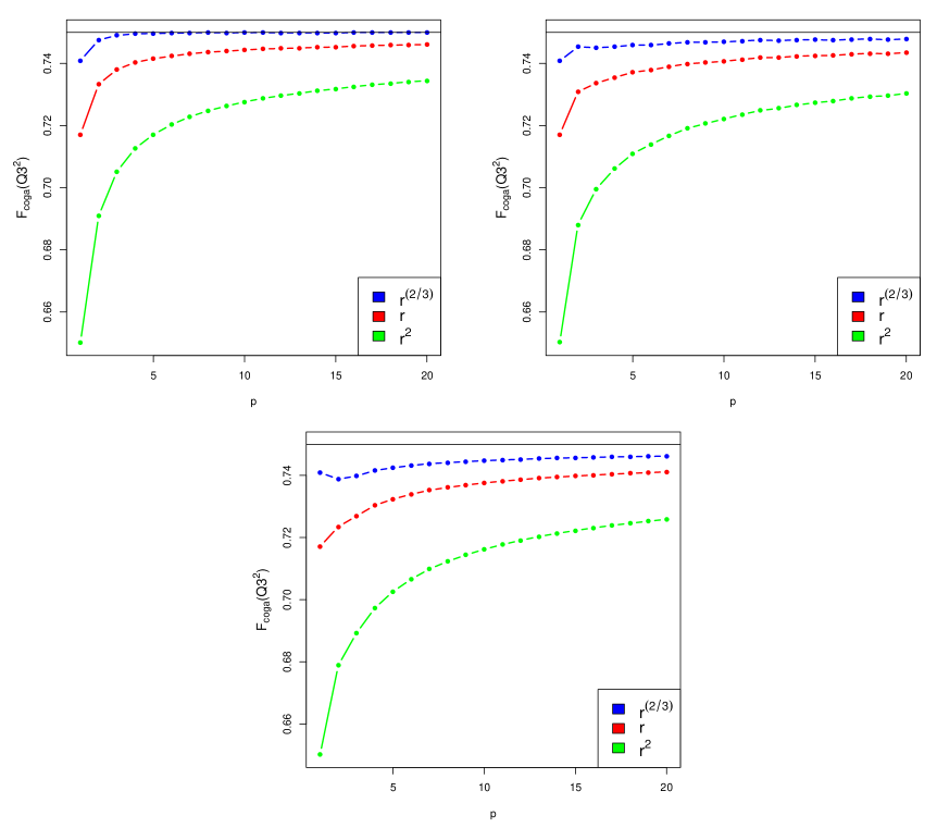
Figure 8: Approximation of the third quartile of a coga distribution for dimensions $p=1,\ldots,20$ when the eigenvalues are constant (top left), linear (top right), or quadratic (bottom), using three different normalizing transforms.

It turns out that the same Wilson-Hilferty transformation also works quite well in the more general situation where the eigenvalues $\lambda_{1},\ldots,\lambda_{p}$ need not be the same. We came to this conclusion by a simulation study, a part of which is illustrated here. The dimension $p$ ranged from 1 to 20 by steps of 1. For each $p$ we generated $n=10^{6}$ observations $y_{1},\ldots,y_{n}$ from the coga distribution with shape parameters $(0.5,\ldots,0.5)$. The scale parameters had three settings: constant $(2,2,\ldots,2)$, linear $(p,(p-1),\ldots,1)$, and quadratic $(p^{2},(p-1)^{2},\ldots,1)$, after which the scale parameters were further standardized in order to sum to $2p$. These correspond to the distribution of the squared Euclidean norms of a multivariate normal distribution where the covariance matrix has eigenvalues that are constant or proportional to $(p,(p-1),\ldots,1)$ (linear eigenvalues) or to $(p^{2},(p-1)^{2},\ldots,1)$ (quadratic eigenvalues). Denote the unsquared Euclidean norms as $r_{i}=\sqrt{y_{i}}$. Then we estimate quantiles, e.g. $Q_{3}$ by assuming normality of the transformed values $h_{1}(r_{i})=r_{i}^{2}$ (square), $h_{2}(r_{i})=r_{i}$ (Fisher), and $h_{3}(r_{i})=r_{i}^{2/3}$ (Wilson-Hilferty), by computing the third quartile of a gaussian distribution with $\hat{\mu}=\mbox{median}_{i}(h(r_{i}))$ and $\hat{\sigma}=\mbox{mad}_{i}(h(r_{i}))$. Finally, we have evaluated the cumulative distribution function of the coga distribution in $\hat{Q}_{3}^{2}$. Ideally, we would like to obtain $F_{\mbox{coga}}(\hat{Q}_{3}^{2})=0.75$. The result of this experiment is shown in Figure 8. We clearly see that the Wilson-Hilferty transform brings the approximate quantile closest to its target value. The results for the first quartile Q1 (not shown) are very similar.

A.2 Proof of Proposition 1

Part 1: Preservation of the eigenvectors.

First note that $g$ is orthogonally equivariant, i.e. $g(HX)=Hg(X)$ for any orthogonal matrix $H$. Therefore $S_{g}=E_{F_{X}}[g(X)g(X)^{T}]$ implies $E_{F_{X}}[g(HX)g(HX)^{T}]=HS_{g}H^{T}$.

The distribution of $Z$ is spherically symmetric hence invariant to reflections along a coordinate axis, which are described by diagonal matrices $R$ with an entry of -1 and all other entries +1. For every reflection matrix $R$ it thus holds that $E_{F_{Z}}[g(DZ)g(DZ)^{T}]=E_{F_{Z}}[g(DRZ)g(DRZ)^{T}]=E_{F_{Z}}[g(RDZ)g(RDZ)^{T}]=RE[g(DZ)g(DZ)^{T}]R^{T}$, where the third equality holds because $DR=RD$ as both $D$ and $R$ are diagonal, and the last equality because R is orthogonal. Therefore $E_{F_{Z}}[g(DZ)g(DZ)^{T}]$ is a diagonal matrix, which we can denote as $\Lambda_{g}:=\mbox{diag}(\lambda_{g,1},\ldots,\lambda_{g,p})$.

Now take $U$ an arbitrary orthogonal matrix and let $X=UDZ$. Then
$S_{g}=E_{F_{Z}}[g(UDZ)g(UDZ)^{T}]=UE_{F_{Z}}[g(DZ)g(DZ)^{T}]U^{T}=U\Lambda_{g}U^{T}$. For the plain covariance matrix $\Sigma$ of X we have $\Sigma=E_{F_{Z}}[UDZ(UDZ)^{T}]=U\Lambda U^{T}$ where $\Lambda=DD^{T}=\mbox{diag}(\delta_{1}^{2},\ldots,\delta_{p}^{2})$. Therefore, the same matrix $U$ orthogonalizes both $\Sigma$ and $S_{g}$ , hence $S_{g}$ and $\Sigma$ have the same eigenvectors.

Part 2: Preservation of the ranks of the eigenvalues.

Let $i>j$ and suppose that $\delta_{i}>\delta_{j}$. We will show that $\lambda_{g,i}>\lambda_{g,j}$. Note that

$$\lambda_{g,i}=\int{g(DZ)_{i}^{2}f_{Z}(Z)dZ}=\int{\delta_{i}^{2}z_{i}^{2}\xi(||DZ||)^{2}f_{Z}(Z)dZ},$$

where $f_{Z}$ is the density of $Z$. Similarly, we have

$$\lambda_{g,j}=\int{g(DZ)_{j}^{2}f_{Z}(Z)dZ}=\int{\delta_{j}^{2}z_{j}^{2}\xi(||DZ||)^{2}f_{Z}(Z)dZ}.$$

This means that $\lambda_{g,i}>\lambda_{g,j}$ is equivalent to:

$$\int{(\delta_{i}^{2}z_{i}^{2}-\delta_{j}^{2}z_{j}^{2})\xi(||DZ||)^{2}f_{Z}(Z)dZ>0}.$$ (A.1)

As $Z$ is spherically symmetric, i.e. $f_{Z}(Z)\sim w(||Z||)$, we can write (A.1) as

$$\int{(\delta_{i}^{2}z_{i}^{2}-\delta_{j}^{2}z_{j}^{2})\xi(||DZ||)^{2}w(||Z||)dZ>0}\;.$$ (A.2)

Note that we can change the variable of integration as follows. Let $y_{k}=\delta_{k}z_{k}$ and write $Y=(y_{1},\ldots,y_{p})$. Then (A.2) is equivalent to

$$\frac{1}{\delta_{1}\cdots\delta_{p}}\left\{\int{(y_{i}^{2}-y_{j}^{2})\xi(||Y||)^{2}w\left(\sqrt{\sum_{k=1}^{p}{\frac{y_{k}^{2}}{\delta_{k}^{2}}}}\right)dY}\right\}>0\;.$$ (A.3)

We can ignore the positive constant $1/(\delta_{1}\cdots\delta_{p})$ and split the integral over the domains $A:=\{x\in\mathbb{R}^{d}|\;|x_{i}|>|x_{j}|\}$ and $B:=\{x\in\mathbb{R}^{d}|\;|x_{i}|<|x_{j}|\}$, yielding

$$\int{(y_{i}^{2}-y_{j}^{2})\xi(||Y||)^{2}w\left(\sqrt{\sum_{k=1}^{p}{\frac{y_{k}^{2}}{\delta_{k}^{2}}}}\right)dY}$$

$$= \int_{A}{(y_{i}^{2}-y_{j}^{2})\xi(||Y||)^{2}w\left(\sqrt{\sum_{k=1}^{p}{\frac{y_{k}^{2}}{\delta_{k}^{2}}}}\right)dY}+\int_{B}{(y_{i}^{2}-y_{j}^{2})\xi(||Y||)^{2}w\left(\sqrt{\sum_{k=1}^{p}{\frac{y_{k}^{2}}{\delta_{k}^{2}}}}\right)dY}$$

$$= \int_{A}{(y_{i}^{2}-y_{j}^{2})\xi(||Y||)^{2}w\left(\sqrt{\sum_{k=1}^{p}{\frac{y_{k}^{2}}{\delta_{k}^{2}}}}\right)dY}+\int_{A}{(y_{j}^{2}-y_{i}^{2})\xi(||Y||)^{2}w\left(\sqrt{\sum_{k=1}^{p}{\frac{y_{k}^{2}}{\delta_{k}^{2}}}+\Delta_{ij}}\right)dY}$$

$$= \int_{A}{(y_{i}^{2}-y_{j}^{2})\xi(||Y||)^{2}\left\{w\left(\sqrt{\sum_{k=1}^{p}{\frac{y_{k}^{2}}{\delta_{k}^{2}}}}\right)-w\left(\sqrt{\sum_{k=1}^{p}{\frac{y_{k}^{2}}{\delta_{k}^{2}}}+\Delta_{ij}}\right)\right\}dY}$$

where in the second equality we have changed the variables of the integration over $B$ by replacing $(y_{i},y_{j})$ by $(-y_{j},y_{i})$ which has Jacobian 1. The $\Delta_{ij}$ in that step is the correction term $\Delta_{ij}=\frac{y_{i}^{2}}{\delta_{j}^{2}}+\frac{y_{j}^{2}}{\delta_{i}^{2}}-\frac{y_{i}^{2}}{\delta_{i}^{2}}-\frac{y_{j}^{2}}{\delta_{j}^{2}}=\frac{y_{i}^{2}-y_{j}^{2}}{\delta_{j}^{2}}-\frac{y_{i}^{2}-y_{j}^{2}}{\delta_{i}^{2}}=(y_{i}^{2}-y_{j}^{2})\left(\frac{1}{\delta_{j}^{2}}-\frac{1}{\delta_{i}^{2}}\right)$.

Note that on $A$ it holds that $|y_{i}|>|y_{j}|$ hence $y_{i}^{2}-y_{j}^{2}>0$ so $\Delta_{ij}>0$. Since $w$ is a decreasing function it follows that

$$w\left(\sqrt{\sum_{k=1}^{p}{\frac{y_{k}^{2}}{\delta_{k}^{2}}}}\right)-w\left(\sqrt{\sum_{k=1}^{p}{\frac{y_{k}^{2}}{\delta_{k}^{2}}}+\Delta_{ij}}\right)>0$$ (A.4)

which implies (A.3) so $\lambda_{g,i}>\lambda_{g,j}$ . If on the other hand $\delta_{i}$ and $\delta_{j}$ are tied, i.e. $\delta_{i}=\delta_{j}$ , it follows that $\Delta_{ij}=0$ hence $\lambda_{g,i}=\lambda_{g,j}$ .

A.3 Influence function

Proof of Proposition 2.

Consider the contaminated distribution $F_{\varepsilon,z}=(1-\varepsilon)F+\varepsilon\Delta_{z}$ where $z\in\mathbb{R}^{p}$ and $\varepsilon\in[0,1]$. We then have:

$$S(F_{\varepsilon,z}) =E_{F_{\varepsilon,z}}\left[g(X)g(X)^{T}\right]$$

$$=(1-\varepsilon)\int{g_{\varepsilon}(X)g_{\varepsilon}(X)^{T}dF(X)}+\varepsilon\int{g_{\varepsilon}(X)g_{\varepsilon}(X)^{T}d\Delta_{z}}\;.$$

If we take the derivative with respect to $\varepsilon$ and evaluate it in $\varepsilon=0$, we get:

$$\left.\frac{\partial}{\partial\varepsilon}S(F_{\varepsilon,z})\right|_{\varepsilon=0}=g(z)g(z)^{T}-\Xi_{g}+\left.\frac{\partial}{\partial\varepsilon}\int{g_{\varepsilon}(X)g_{\varepsilon}(X)^{T}dF(X)}\right|_{\varepsilon=0}\;.$$

Calculation of the IF.

While the expression of the influence function might seem relatively simple, its (numerical) calculation is rather involved. We can write:

$$\left.\frac{\partial}{\partial\varepsilon}\int{g_{\varepsilon}(X)g_{\varepsilon}(X)^{T}dF(X)}\right|_{\varepsilon=0}$$

$$= \left.\int{\frac{\partial}{\partial\varepsilon}\left(g_{\varepsilon}(X)\right)g_{\varepsilon}(X)^{T}+g_{\varepsilon}(X)\frac{\partial}{\partial\varepsilon}\left(g_{\varepsilon}(X)^{T}\right)dF(X)}\right|_{\varepsilon=0}$$

$$= \int{\left(\left.\frac{\partial}{\partial\varepsilon}g_{\varepsilon}(X)\right|_{\varepsilon=0}\right)g(X)^{T}+g(X)\left(\left.\frac{\partial}{\partial\varepsilon}g_{\varepsilon}(X)^{T}\right|_{\varepsilon=0}\right)dF(X)}.$$

So the term we need to determine is $\left.\frac{\partial}{\partial\varepsilon}g_{\varepsilon}(X)\right|_{\varepsilon=0}$. Recalling that $g(t)=t\xi(||t||)$ we have $g_{\varepsilon}(t)=t\xi_{\varepsilon}(||t||)$. This means that the contamination affects $g$ because it affects the radial function $\xi$. Therefore we have to compute $\left.\frac{\partial}{\partial\varepsilon}g_{\varepsilon}(X)\right|_{\varepsilon=0}=X\left.\frac{\partial}{\partial\varepsilon}\xi_{\varepsilon}(||X||)\right|_{\varepsilon=0}$ for the functions $g$ given by (4)–(8).

In these functions $\xi$ depends on $F_{X}$ though the distribution of $||X||^{2/3}$. Suppose that $||X||^{2/3}\sim G$ when $X\sim F$, so $G$ is a univariate distribution. For $X_{\varepsilon}\sim F_{\varepsilon,z}=(1-\varepsilon)F+\varepsilon\Delta_{z}$ we then have $||X_{\varepsilon}||^{2/3}\sim G_{\varepsilon,||z||^{2/3}}=(1-\varepsilon)G+\varepsilon\Delta_{||z||^{2/3}}$ . For uncontaminated data the density of $||X||^{2/3}$ is given by

$$f_{G}(t)=f_{\mbox{coga}}(t^{3})|3t^{2}|\;,$$

where $f_{\mbox{coga}}$ is the density of the convolution of gamma distributions. We need this density to evaluate the influence functions of their median and mad.

The cutoffs in the paper are

$$Q_{1} = \left(\mbox{hmed}{||X||^{\frac{2}{3}}}-\mbox{hmad}{||X||^{\frac{2}{3}}}\right)^{\frac{3}{2}}$$

$$Q_{2} = \left(\mbox{hmed}{||X||^{\frac{2}{3}}}\right)^{\frac{3}{2}}$$

$$Q_{3} = \left(\mbox{hmed}{||X||^{\frac{2}{3}}}+\mbox{hmad}{||X||^{\frac{2}{3}}}\right)^{\frac{3}{2}}$$

$$Q_{3}^{*} = \left(\mbox{hmed}{||X||^{\frac{2}{3}}}+1.4826\;\mbox{hmad}{||X||^{\frac{2}{3}}}\right)^{\frac{3}{2}}$$

and we can compute their influence functions:

$$\mbox{IF}(z,Q_{1},F)= \;\frac{3}{2}\sqrt{\mbox{median}(G)-\;\mbox{mad}(G)}\;(\mbox{IF}(||z||^{2/3},\mbox{median},G)-\;\mbox{IF}(||z||^{2/3},\mbox{mad},G))$$

$$\mbox{IF}(z,Q_{2},F)= \;\frac{3}{2}\sqrt{\mbox{median}(G)}\;\mbox{IF}(||z||^{2/3},\mbox{median},G)$$

$$\mbox{IF}(z,Q_{3},F)= \;\frac{3}{2}\sqrt{\mbox{median}(G)+\;\mbox{mad}(G)}\;(\mbox{IF}(||z||^{2/3},\mbox{median},G)+\;\mbox{IF}(||z||^{2/3},\mbox{mad},G))$$

$$\mbox{IF}(z,Q_{3}^{*},F)= \;\frac{3}{2}\sqrt{\mbox{median}(G)+1.4826\;\mbox{mad}(G)}\;(\mbox{IF}(||z||^{2/3},\mbox{median},G)$$

$$\;+1.4826\;\mbox{IF}(||z||^{2/3},\mbox{mad},G)).$$

The Winsor GSSCM is given by $\xi(r)=\mathbbm{1}_{r\leqslant Q_{2}}+\frac{Q_{2}}{r}\mathbbm{1}_{r>Q_{2}}$. For the contaminated case this becomes $\xi_{\varepsilon}(r)=\mathbbm{1}_{r\leqslant Q_{2,\varepsilon}}+\frac{Q_{2,\varepsilon}}{r}\mathbbm{1}_{r>Q_{2,\varepsilon}}$. We then have:

$$\frac{\partial}{\partial\varepsilon}\xi_{\varepsilon}(r) =\frac{\partial}{\partial\varepsilon}\left\{\mathbbm{1}_{[0,Q_{2,\varepsilon}]}(r)+\frac{Q_{2,\varepsilon}}{r}\mathbbm{1}_{(Q_{2,\varepsilon},\infty)}(r)\right\}$$

$$=\delta(r-Q_{2,\varepsilon})Q_{2,\varepsilon}^{\prime}+\frac{Q_{2,\varepsilon}^{\prime}}{r}\mathbbm{1}_{(Q_{2,\varepsilon},\infty)}(r)-\frac{Q_{2,\varepsilon}}{r}\delta(r-Q_{2,\varepsilon})Q_{2,\varepsilon}^{\prime}\;,$$

where $\delta(x-y)$ denotes the distributional derivative of $\mathbbm{1}_{(-\infty,x]}(y)$. Evaluation in $\varepsilon=0$ gives

$$\delta(r-Q_{2})IF(z,Q_{2},F)+\frac{\mbox{IF}(z,Q_{2},F)}{r}\mathbbm{1}_{(Q_{2},\infty)}(r)-\frac{Q_{2}}{r}\delta(r-Q_{2})IF(z,Q_{2},F)$$

$$=\left(1-\frac{Q_{2}}{r}\right)\delta(r-Q_{2})IF(z,Q_{2},F)+\frac{\mbox{IF}(z,Q_{2},F)}{r}\mathbbm{1}_{(Q_{2},\infty)}(r)\;.$$

As $\left(1-\frac{Q_{2}}{r}\right)\delta(r-Q_{2})$ is 0 everywhere, we only need to integrate the last term. This yields

$$\left.\frac{\partial}{\partial\varepsilon}g_{\varepsilon}(X)\right|_{\varepsilon=0}=\frac{X}{||X||}\mbox{IF}(z,Q_{2},F)\mathbbm{1}_{(Q_{2},\infty)}(||X||)\;.$$

The influence function of $S_{g}$ is thus given by:

$$\mbox{IF}(z,S_{g},F)= g(z)g(z)^{T}-\Xi_{g}(F)$$

$$+\int{\left(\frac{X}{||X||}\mbox{IF}(z,Q_{2},F)\mathbbm{1}_{(Q_{2},\infty)}(||X||)\right)g(X)^{T}dF(X)}$$

$$+\int{g(X)\left(\frac{X}{||X||}\mbox{IF}(z,Q_{2},F)\mathbbm{1}_{(Q_{2},\infty)}(||X||)\right)^{T}dF(X)}.$$

Note that the last 2 terms in the sum are each other’s transpose. The integration is done numerically.

The derivation of the influence function of the Quad GSSCM is entirely similar to that of Winsor. The main difference is that now $\left.\frac{\partial}{\partial\varepsilon}g_{\varepsilon}(X)\right|_{\varepsilon=0}$ is given by

$$\left.\frac{\partial}{\partial\varepsilon}g_{\varepsilon}(X)\right|_{\varepsilon=0}=2Q_{2}\mbox{IF}(z,Q_{2},F)\frac{X}{||X||^{2}}\mathbbm{1}_{(Q_{2},\infty)}(||X||)\;.$$

The linearly redescending (LR) method uses a second cutoff:

$$\xi(r)=\begin{cases}1&\mbox{ if }r\leqslant Q_{2}\\ (Q_{3}^{*}-r)/(Q_{3}^{*}-Q_{2})&\mbox{ if }Q_{2}<r\leqslant Q_{3}^{*}\\ 0&\mbox{ if }r>Q_{3}^{*}\;.\end{cases}$$ (A.5)

In the contaminated case we obtain $g_{\varepsilon}(x)=x\xi_{\varepsilon}(||x||)$ with

$$\xi_{\varepsilon}(r)=\begin{cases}1&\mbox{ if }r\leqslant Q_{2,\varepsilon}\\ (Q_{3,\varepsilon}^{*}-r)/(Q_{3,\varepsilon}^{*}-Q_{2,\varepsilon})&\mbox{ if }Q_{2,\varepsilon}<r\leqslant Q_{3,\varepsilon}^{*}\\ 0&\mbox{ if }r>Q_{3,\varepsilon}^{*}\;.\end{cases}$$ (A.6)

Taking the derivative with respect to $\varepsilon$ yields:

$$\frac{\partial}{\partial\varepsilon}\xi_{\varepsilon}(r) =\delta(r-Q_{2,\varepsilon})+\frac{Q_{3,\varepsilon}^{*}-r}{Q_{3,\varepsilon}^{*}-Q_{2,\varepsilon}}\left(\delta(r-Q_{3,\varepsilon}^{*})-\delta(r-Q_{2,\varepsilon})\right)$$

$$+\mathbbm{1}_{[Q_{2,\varepsilon},Q_{3,\varepsilon}^{*}]}\frac{Q_{3,\varepsilon}^{*\prime}(Q_{3,\varepsilon}^{*}-Q_{2,\varepsilon})-(Q_{3,\varepsilon}^{*\prime}-Q_{2,\varepsilon}^{\prime})(Q_{3,\varepsilon}^{*}-r)}{(Q_{3,\varepsilon}^{*}-Q_{2,\varepsilon})^{2}}\;.$$

Evaluation in $\varepsilon=0$ gives:

$$\delta(r-Q_{2})+\frac{Q_{3}^{*}-r}{Q_{3}^{*}-Q_{2}}\left(\delta(r-Q_{3}^{*})-\delta(r-Q_{2})\right)$$

$$+\mathbbm{1}_{[Q_{2},Q_{3}^{*}]}\frac{\mbox{IF}(z,Q_{3}^{*},F)(Q_{3}^{*}-Q_{2})-(\mbox{IF}(z,Q_{3}^{*},F)-\mbox{IF}(z,Q_{2},F))(Q_{3}^{*}-r)}{(Q_{3}^{*}-Q_{2})^{2}}\;.$$

When integrating only the last term plays a role, yielding

$$\left.\frac{\partial}{\partial\varepsilon}g_{\varepsilon}(X)\right|_{\varepsilon=0}= X\mathbbm{1}_{[Q_{2},Q_{3}^{*}]}(||X||)$$

$$\frac{\mbox{IF}(||z||,Q_{3}^{*},F)(Q_{3}^{*}-Q_{2})-(\mbox{IF}(||z||,Q_{3}^{*},F)-\mbox{IF}(||z||,Q_{2},F))(Q_{3}^{*}-||X||)}{(Q_{3}^{*}-Q_{2})^{2}}$$

$$= X\mathbbm{1}_{[Q_{2},Q_{3}^{*}]}(||X||)\frac{\mbox{IF}(||z||,Q_{3}^{*},F)(||X||-Q_{2})+\mbox{IF}(||z||,Q_{2},F)(Q_{3}^{*}-||X||)}{(Q_{3}^{*}-Q_{2})^{2}}\;.$$

For the Ball SSCM we analogously derive that

$$\left.\frac{\partial}{\partial\varepsilon}g_{\varepsilon}(X)\right|_{\varepsilon=0}=\delta(||X||-Q_{2})\mbox{IF}(z,Q_{2},F)X\;.$$

Finally, for the Shell SSCM we obtain

$$\left.\frac{\partial}{\partial\varepsilon}g_{\varepsilon}(X)\right|_{\varepsilon=0}=\left(\delta(||X||-Q_{3})\mbox{IF}(z,Q_{3},F)-\delta(||X||-Q_{1})\mbox{IF}(z,Q_{1},F)\right)X\;.$$

A.4 Breakdown values

Proof of Proposition 3.

Proof.

Denote by $\mathcal{J}$ the set of all subsets of $\{1,\ldots,n\}$ with $p+1$ elements. For every subset $J\in\mathcal{J}$ we define $\displaystyle\eta_{J}\coloneqq\max_{i\in J}{d^{2}(x_{i},H_{J})}$, where $H_{J}$ is the hyperplane minimizing $\displaystyle\sum_{i\in J}{d^{2}(x_{i},H)}$ over all possible hyperplanes $H$ and $d(x,H)$ is the Euclidean distance between a point $x$ and a hyperplane $H$. Define $\displaystyle\eta_{\bm{X}}\coloneqq\min_{J\in\mathcal{J}}{\eta_{J}}$. Since the original points $\{x_{1},\ldots,x_{n}\}$ are in general position, no $p+1$ points can lie on the same hyperplane, which ensures that $\eta_{\bm{X}}>0$. We also put $c_{1}\coloneqq\max_{i}||x_{i}-T(\bm{X})||<\infty$.

Part 1. We first need to show that $\epsilon^{*}\geqslant\left\lfloor(n-p+1)/2\right\rfloor/n$.

Let $m<\left\lfloor(n-p+1)/2\right\rfloor$ and replace $m$ observations of $\bm{X}=\{x_{1},\ldots,x_{n}\}$ yielding $\bm{X}^{*}$ with location estimate $T(\bm{X}^{*})$. Because $\frac{m}{n}$ is below the breakdown value of $T$, there is a constant $c_{2}<\infty$ so that $||T(\bm{X}^{*})-T(\bm{X})||\leqslant c_{2}$ for all such contaminated datasets $\bm{X}^{*}$. By the triangle inequality $||x_{i}-T(\bm{X}^{*})||\leqslant c_{1}+c_{2}<\infty$. This implies $\mbox{hmed}(d_{i}^{*})\leqslant c_{1}+c_{2}$ , hence $\mbox{hmed}(d_{i}^{*})+1.4826\,\mbox{hmad}(d_{i}^{*})\leqslant 2.4826\;\mbox{hmed}(d_{i}^{*})\leqslant 2.4826(c_{1}+c_{2})$, where $d_{i}^{*}=||x_{i}^{*}-T(\bm{X}^{*})||$. Therefore $||g(t)||\leqslant 2.4826(c_{1}+c_{2})$ by condition 3.

First we show that the largest eigenvalue of $S_{g}(\bm{X}^{*})$ is bounded over all such datasets $\bm{X}^{*}$. Take any $\bm{X}^{*}$, obtained by replacing $m$ points of $\bm{X}$ by arbitrary points. Then

$$\lambda_{\mbox{max}} =\sup_{||u||=1}{u^{T}S_{g}(\bm{X}^{*})u}=\sup_{||u||=1}\frac{1}{n}\sum_{i=1}^{n}{u^{T}g(x_{i}^{*}-T(\bm{X}^{*}))g(x_{i}^{*}-T(\bm{X}^{*}))^{T}u}$$

$$=\sup_{||u||=1}\frac{1}{n}\sum_{i=1}^{n}{\left(u^{T}g(x_{i}^{*}-T(\bm{X}^{*}))\right)^{2}}\leqslant\sup_{||u||=1}\frac{1}{n}\sum_{i=1}^{n}{||u||^{2}||g(x_{i}^{*}-T(\bm{X}^{*}))||^{2}}$$

$$\leqslant(2.4826(c_{1}+c_{2}))^{2}<\infty.$$

Next we show that the smallest eigenvalue of $S_{g}(\bm{X}^{*})$ has a positive lower bound for all contaminated datasets $\bm{X}^{*}$. By condition 2 on $\xi$ we know that $\#\{x_{i}|\;\xi(||x_{i}-T(\bm{X}^{*})||)=1\}\geqslant\left\lfloor(n+p+1)/2\right\rfloor$. Therefore, we have at least $\left\lfloor(n+p+1)/2\right\rfloor-(\left\lfloor(n-p+1)/2\right\rfloor-1)=p+1$ regular points for which $\xi(||x_{i}-T(\bm{X}^{*})||)=1$, let’s assume w.l.o.g. that these are $x_{1},\ldots,x_{p+1}$. We can now write

$$\lambda_{\mbox{min}}=\min_{||u||=1}{u^{T}S_{g}(\bm{X}^{*})u} =\min_{||u||=1}\frac{1}{n}\sum_{i=1}^{n}{u^{T}g(x_{i}^{*}-T(\bm{X}^{*}))g(x_{i}^{*}-T(\bm{X}^{*}))^{T}u}$$

$$=\min_{||u||=1}\frac{1}{n}\sum_{i=1}^{n}{\left(u^{T}g(x_{i}^{*}-T(\bm{X}^{*}))\right)^{2}}$$

$$\geqslant\min_{||u||=1}\frac{1}{n}\sum_{i=1}^{p+1}{\left(u^{T}(x_{i}-T(\bm{X}^{*}))\xi(x_{i}-T(\bm{X}^{*}))\right)^{2}}$$

$$=\min_{||u||=1}\frac{1}{n}\sum_{i=1}^{p+1}{\left(u^{T}(x_{i}-T(\bm{X}^{*}))\right)^{2}}$$

$$\geqslant\frac{1}{n}\sum_{i=1}^{p+1}{d^{2}(x_{i},H_{\{1,\ldots,p+1\}})}\geqslant\eta_{\bm{X}}>0\;.$$

Part 2. It remains to show that $\epsilon^{*}\leqslant\left\lfloor(n-p+1)/2\right\rfloor/n$. This is the known upper bound for affine equivariant scatter estimators but that result doesn’t apply here, so we need to show it for this case. Take any $m\geqslant\left\lfloor(n-p+1)/2\right\rfloor$ and replace the last $m$ points of $\bm{X}$, keeping the points $x_{1},\ldots,x_{n-m}$ unchanged. By location equivariance we can assume w.l.o.g. that the average of $x_{1},\ldots,x_{n-m}$ is zero. For $j=n-m+1,\ldots,n$ put $x_{j}^{*}=\lambda a_{j}$ where $a_{j}$ is such that $\min_{i=n-m+1,\ldots,n}{||a_{j}-a_{i}||}\geqslant 1$ and such that for all $\lambda>1$ it holds that $\min_{i=1,\ldots,n-m}{||\lambda a_{j}-x_{i}||}\geqslant\lambda$. This is possible by placing the $a_{j}$ outside of the convex hull of $\bm{X}$ and far enough from each other and $\bm{X}$.

Now consider an unbounded increasing sequence of $\lambda_{k}>1$. For every $\lambda_{k}$ the set $\{x_{n-m+1}^{*},\ldots,x_{n}^{*}\}$ must contain at least one point for which $w_{i}=1$, call this point $x_{b}^{*}$. Take another point of $\bm{X}^{*}$ for which $w_{i}=1$, name this $x_{c}^{*}$. Note that $x^{*}_{c}$ can be an original data point or a replaced point. We now have that $||x_{b}^{*}-x_{c}^{*}||\geqslant\lambda$ hence $||x_{b}^{*}-T(\bm{X}^{*})||+||x_{c}^{*}-T(\bm{X}^{*})||\geqslant\lambda$. Therefore $||x_{b}^{*}-T(\bm{X}^{*})||^{2}+||x_{c}^{*}-T(\bm{X}^{*})||^{2}\geqslant\lambda^{2}/2$. We then obtain

$$\sum_{j=1,\ldots,p}\lambda_{j}(S(\bm{X}^{*})) =\mbox{trace}(S(\bm{X}^{*}))$$

$$=\frac{1}{n}\sum_{i=1,\ldots,n}\mbox{trace}((x_{i}^{*}-T(\bm{X}^{*}))(x_{i}^{*}-T(\bm{X}^{*}))^{T})$$

$$=\frac{1}{n}\sum_{i=1,\ldots,n}||x_{i}^{*}-T(\bm{X}^{*})||^{2}$$

$$\geqslant\frac{1}{n}(||x_{b}^{*}-T(\bm{X}^{*})||^{2}+||x_{c}^{*}-T(\bm{X}^{*})||^{2})$$

$$\geqslant\lambda^{2}/(2n)\;.$$

This becomes arbitrarily large and so $S(\bm{X}^{*})$ explodes. ∎

Proof of Proposition 4.

Proof.

Showing that $\varepsilon^{*}(T,\bm{X})\leqslant\left\lfloor(n+1)/2\right\rfloor/n$ is easy, since $\left\lfloor(n+1)/2\right\rfloor/n$ is the upper bound on the breakdown value of all translation equivariant location estimators, see e.g. Lopuhaä and Rousseeuw (1991).

It remains to show that $\varepsilon^{*}(T,\bm{X})\geqslant\left\lfloor(n+1)/2\right\rfloor/n$.

Note that the objective given by the sum of the $h$ smallest squared Euclidean distances is nonincreasing in every C-step. The value of the objective function after step $k$ is $\sum_{j=1}^{h}{d_{(j)}^{2}(\bm{X},T_{k}(\bm{X}))}$ where $d_{(j)}(\bm{X},T_{k}(\bm{X}))$ denotes the $j$-th order statistic of the distances $||x_{i}-T_{k}(\bm{X})||$, and we have that $\sum_{j=1}^{h}{d_{(j)}^{2}(\bm{X},T_{k}(\bm{X}))}\leqslant\sum_{j=1}^{h}{d_{(j)}^{2}(\bm{X},T_{k-1}(\bm{X}))}$.

Recall that $h=\left\lfloor(n+1)/2\right\rfloor$ and define $c_{1}\coloneqq\max_{i}{||x_{i}-T_{k}(\bm{X})||}<\infty$. Let $m<n-h$ and replace w.l.o.g. the last $m$ observations of $\bm{X}=\{x_{1},\ldots,x_{n}\}$ to obtain $\bm{X}^{*}=\{x_{1},\ldots,x_{n-m},x_{n-m+1}^{*},\ldots,x_{n}^{*}\}=\{x_{1}^{*},\ldots,x_{n}^{*}\}$. Since the spatial median $T_{0}$ does not yet break down for this $m$ (Lopuhaä and Rousseeuw, 1991), there is a constant $c_{2}$ such that $\max_{i}{||x_{i}-T_{0}(\bm{X}^{*})||}\leqslant c_{2}<\infty$ for all such datasets $\bm{X}^{*}$.

Consider $T_{k}(\bm{X}^{*})$ and the corresponding objective function $\sum_{j=1}^{h}{d_{(j)}^{2}(\bm{X}^{*},T_{k}(\bm{X}^{*}))}$. Since the C-step does not increase the value of the objective function, we have that

$$\sum_{j=1}^{h}{d_{(j)}^{2}(\bm{X}^{*},T_{k}(\bm{X}^{*}))}\leqslant\sum_{j=1}^{h}{d_{(j)}^{2}(\bm{X}^{*},T_{k-1}(\bm{X}^{*}))}\leqslant\ldots\leqslant\sum_{j=1}^{h}{d_{(j)}^{2}(\bm{X}^{*},T_{0}(\bm{X}^{*}))}.$$

Note that

$$\sum_{j=1}^{h}{d_{(j)}^{2}(\bm{X}^{*},T_{0}(\bm{X}^{*}))} \leqslant\sum_{i=1}^{h}{||x_{i}^{*}-T_{0}(\bm{X}^{*})||^{2}}=\sum_{i=1}^{h}{||x_{i}-T_{0}(\bm{X}^{*})||^{2}}$$

$$\leqslant\left(\sum_{i=1}^{h}{||x_{i}-T_{0}(\bm{X}^{*})||}\right)^{2}\leqslant\left(hc_{2}\right)^{2}.$$

Since $m$ is at most $\left\lfloor(n-1)/2\right\rfloor$ and $h=\left\lfloor(n+1)/2\right\rfloor$ we have at least $\left\lfloor(n+1)/2\right\rfloor-\left\lfloor(n-1)/2\right\rfloor=1$ point $x_{j}$ with $1\leqslant j\leqslant n-m$ for which $||x_{j}-T_{k}(\bm{X}^{*})||^{2}\leqslant d_{(h)}^{2}(\bm{X}^{*},T_{k}(\bm{X}^{*}))$. Note that $||x_{j}-T_{k}(\bm{X}^{*})||^{2}\leqslant\sum_{j=1}^{h}{d_{(j)}^{2}(\bm{X}^{*},T_{k}(\bm{X}^{*}))}\leqslant\sum_{j=1}^{h}{d_{(j)}^{2}(\bm{X}^{*},T_{0}(\bm{X}^{*}))}$. So for this $x_{j}$ we can write

$$||T_{k}(\bm{X}^{*})-T_{0}(\bm{X})|| \leqslant||T_{k}(\bm{X}^{*})-x_{j}||+||x_{j}-T_{0}(\bm{X})||$$

$$\leqslant hc_{2}+c_{1}<\infty\;.$$

Note that this upper bound does not depend on $k$ and therefore remains valid when the procedure is iterated until convergence ($k\rightarrow\infty$). ∎

References

• Boente et al. (2018) Boente, G., D. Rodriguez, and M. Sud (2018). The spatial sign operator: Asymptotic results and applications. arXiv:1804.04210v1.
• Brown (1983) Brown, B. M. (1983). Statistical uses of the spatial median. Journal of the Royal Statistical Society, Series B 45(1), 25–30.
• Chatzinakos et al. (2016) Chatzinakos, C., L. Pitsoulis, and G. Zioutas (2016). Optimization techniques for robust multivariate location and scatter estimation. Journal of Combinatorial Optimization 31(4), 1443–1460.
• Croux et al. (2010) Croux, C., C. Dehon, and A. Yadine (2010). The k-step spatial sign covariance matrix. Advances in Data Analysis and Classification 4(2), 137–150.
• Croux et al. (2002) Croux, C., E. Ollila, and H. Oja (2002). Sign and rank covariance matrices: Statistical properties and application to principal components analysis. In Y. Dodge (Ed.), Statistical Data Analysis Based on the L1-Norm and Related Methods, Basel, pp.  257–269. Birkhäuser Basel.
• Donoho and Huber (1983) Donoho, D. and P. Huber (1983). The notion of breakdown point. In P. Bickel, K. Doksum, and J. Hodges (Eds.), A Festschrift for Erich Lehmann, Belmont, pp.  157–184. Wadsworth.
• Dürre et al. (2017) Dürre, A., R. Fried, and D. Vogel (2017). The spatial sign covariance matrix and its application for robust correlation estimation. Austrian Journal of Statistics 46(3-4), 13–22.
• Dürre et al. (2016) Dürre, A., D. E. Tyler, and D. Vogel (2016). On the eigenvalues of the spatial sign covariance matrix in more than two dimensions. Statistics & Probability Letters 111, 80 – 85.
• Dürre and Vogel (2016) Dürre, A. and D. Vogel (2016). Asymptotics of the two-stage spatial sign correlation. Journal of Multivariate Analysis 144, 54 – 67.
• Dürre et al. (2015) Dürre, A., D. Vogel, and R. Fried (2015). Spatial sign correlation. Journal of Multivariate Analysis 135, 89 – 105.
• Dürre et al. (2014) Dürre, A., D. Vogel, and D. E. Tyler (2014). The spatial sign covariance matrix with unknown location. Journal of Multivariate Analysis 130, 107 – 117.
• Gower (1974) Gower, J. C. (1974). Algorithm AS 78: The Mediancentre. Journal of the Royal Statistical Society Series C (Applied Statistics) 23(3), 466–470.
• Hampel et al. (1986) Hampel, F., E. Ronchetti, P. Rousseeuw, and W. Stahel (1986). Robust Statistics: The Approach Based on Influence Functions. New York: Wiley.
• Hu et al. (2018) Hu, C., V. Pozdnyakov, and J. Yan (2018). Coga: Convolution of Gamma Distributions. University of Connecticut. R package version 0.2.2.
• Hubert et al. (2005) Hubert, M., P. J. Rousseeuw, and K. Vanden Branden (2005). ROBPCA: A New Approach to Robust Principal Component Analysis. Technometrics 47(1), 64-79.
• Hubert et al. (2012) Hubert, M., P. J. Rousseeuw, and T. Verdonck (2012). A deterministic algorithm for robust location and scatter. Journal of Computational and Graphical Statistics 21(3), 618–637.
• Locantore et al. (1999) Locantore, N., J. S. Marron, D. G. Simpson, N. Tripoli, J. T. Zhang, and K. L. Cohen (1999). Robust principal component analysis for functional data. Test 8(1), 1–28.
• Lopuhaä and Rousseeuw (1991) Lopuhaä, H. and P. Rousseeuw (1991). Breakdown points of affine equivariant estimators of multivariate location and covariance matrices. The Annals of Statistics 19, 229–248.
• Magyar and Tyler (2014) Magyar, A. F. and D. E. Tyler (2014). The asymptotic inadmissibility of the spatial sign covariance matrix for elliptically symmetric distributions. Biometrika 101(3), 673–688.
• Marden (1999) Marden, J. I. (1999). Some robust estimates of principal components. Statistics & Probability Letters 43(4), 349 – 359.
• Moschopoulos (1985) Moschopoulos, P. G. (1985). The distribution of the sum of independent gamma random variables. Annals of the Institute of Statistical Mathematics 37(1), 541–544.
• Mozharovskyi et al. (2015) Mozharovskyi, P., K. Mosler and T. Lange (2015). Classifying real-world data with the DD$\alpha$-procedure. Advances in Data Analysis and Classification 9(3), 287–314.
• Pokotylo et al. (2016) Pokotylo, O., P. Mozharovskyi and R. Dyckerhoff (2016). Depth and depth-based classification with R-package ddalpha. arXiv:1608.04109
• Reaven and Miller (1979) Reaven, G. M. and R. G. Miller (1979). An attempt to define the nature of chemical diabetes using a multidimensional analysis. Diabetologia 16, 17–24.
• Rocke (1996) Rocke, D. M. (1996). Robustness properties of S-estimators of multivariate location and shape in high dimension. The Annals of Statistics 24(3), 1327–1345.
• Rousseeuw (1984) Rousseeuw, P. (1984). Least median of squares regression. Journal of the American Statistical Association 79, 871–880.
• Rousseeuw and Van Driessen (1999) Rousseeuw, P. and K. Van Driessen (1999). A fast algorithm for the Minimum Covariance Determinant estimator. Technometrics 41, 212–223.
• Serneels et al. (2006) Serneels, S., E. De Nolf, and P. J. Van Espen (2006). Spatial sign preprocessing: a simple way to impart moderate robustness to multivariate estimators. Journal of Chemical Information and Modeling 46(3), 1402–1409. PMID: 16711760.
• Sirkia et al. (2009) Sirkia, S., S. Taskinen, H. Oja, and D. E. Tyler (2009). Tests and estimates of shape based on spatial signs and ranks. Journal of Nonparametric Statistics 21(2), 155–176.
• Taskinen et al. (2012) Taskinen, S., I. Koch, and H. Oja (2012). Robustifying principal component analysis with spatial sign vectors. Statistics & Probability Letters 82(4), 765 – 774.
• Visuri et al. (2000) Visuri, S., V. Koivunen, and H. Oja (2000). Sign and rank covariance matrices. Journal of Statistical Planning and Inference 91(2), 557 – 575.
• Visuri et al. (2001) Visuri, S., H. Oja, and V. Koivunen (2001). Subspace-based direction-of-arrival estimation using nonparametric statistics. IEEE Transactions on Signal Processing 49(9), 2060–2073.
• Wilson and Hilferty (1931) Wilson, E. B. and M. M. Hilferty (1931). The distribution of chi-square. Proceedings of the National Academy of Sciences of the United States of America 17, 684 – 688.