Geometric Dynamics of a Harmonic Oscillator,
Arbitrary Minimal Uncertainty States
and the Smallest Step $3$ Nilpotent Lie Group

Abstract.

The paper presents a new method of geometric solution of a Schrödinger equation by constructing an equivalent first-order partial differential equation with a bigger number of variables. The equivalent equation shall be restricted to a specific subspace with auxiliary conditions which are obtained from a coherent state transform. The method is applied to the fundamental case of the harmonic oscillator and coherent state transform generated by the minimal nilpotent step three Lie group—the group $\mathbb{G}$ (also known under many names, e.g. quartic group). We obtain a geometric solution for an arbitrary minimal uncertainty state used as a fiducial vector. In contrast, it is shown that the well-known Fock–Segal–Bargmann transform and the Heisenberg group require a specific fiducial vector to produce a geometric solution. A technical aspect considered in this paper is that a certain modification of a coherent state transform is required: although the irreducible representation of the group $\mathbb{G}$ is square-integrable modulo a subgroup $H$, the obtained dynamic is transverse to the homogeneous space $\mathbb{G}/H$.

1. Introduction

A transition from configuration space to the phase space in quantum mechanics is performed by the coherent states transform [deGosson11a, deGosson06a, Folland89]. As a result the number of independent variables is doubled from $\mathbb{R}^{n}{}$ to $\mathbb{C}^{n}{}$ and an irreducible Fock–Segal–Bargmann space is characterised by the analyticity condition [Vourdas06a, Kisil17a]. The dynamic of quantum harmonic oscillator in Fock–Segal–Bargmann space is given geometrically as one-parameter subgroup of symplectomorphisms. In this paper we describe a method generalising this construction of geometric solutions of the Schrödinger equation.

The technique is applied to obtain a novel picture of a harmonic oscillator dynamics associated to squeezed states. The harmonic oscillator is an archetypal example of exactly solvable classical and quantum systems with applications to many branches of physics, e.g. optics [Wolf10a]. However, not only the solution of harmonic oscillator has numerous uses, important methods with a wide applicability were initially tested on this fundamental case. The most efficient solution of the spectral problem through ladder operators were successfully expanded from the harmonic oscillator to hydrogen atom [Schrodinger40a] with further generalisations in supersymmetric quantum mechanics [CarinenaPlyushchay17a] and pseudo-boson framework [AliBagarelloGazeau15a].

In order to clarify our target we need to recall briefly the scheme with an emphasis on some details which are usually depressed in abridged presentations. Let the quantum observables for coordinate $q$ and momentum $p$ satisfy the Heisenberg canonical commutator relation (CCR):

(1.1) $$[q,p]=\mathrm{i}\hslash I\,.$$

Then, for a harmonic oscillator with the mass $m$ and frequency $\omega$ one introduces the ladder (annihilation and creation) operators $(a^{-},a^{+})$:

(1.2) $$a^{\pm}=\sqrt{\frac{m\omega}{2\hslash}}\left(q\mp\frac{\mathrm{i}}{m\omega}p\right)\quad\text{ with the commutator }[a^{-},a^{+}]=I.$$

Thereafter, the Hamiltonian $H$ of the harmonic oscillator can be expressed through the ladder operators:

(1.3) $$H=\frac{1}{2}\left(\frac{1}{m}p^{2}+m\omega^{2}q^{2}\right)=\hslash\omega\left(a^{+}a^{-}+\frac{1}{2}\right)\,.$$

Assuming the existence of a non-zero vacuum $\phi_{0}$ such that $a^{-}\phi_{0}=0$, the commutator relations (1.2) imply that states $\phi_{n}=(a^{+})^{n}\phi_{0}$ are eigenvectors of $H$ with eigenvalues $n+\frac{1}{2}$. This completely solves the spectral problem for the harmonic oscillator, but a couple of observations are in place:

1. The ladder operators (1.2) (and subsequently the eigenvectors $\phi_{n}$) depend on the parameter $m\omega$. They are not useful for a harmonic oscillator with a different value of $m^{\prime}\omega^{\prime}$.

2. The explicit dynamic of an arbitrary state $f$ is not transparent: first we need to find its decomposition $f=\sum_{n}c_{n}\phi_{n}$ over the orthogonal basis of eigenvectors $\phi_{n}$ and then express evolution as

   (1.4) $$F(t)=\sum_{n}c_{n}\mathrm{e}^{-\mathrm{i}(n+\frac{1}{2})\omega t}\phi_{n}\,.$$

The latter can be fixed by the coherent states transform to Fock–Segal–Bargmann (FSB) space [Folland89]*1.6:

(1.5) $$\mathcal{W}_{\phi_{0}}:\;f\rightarrow\tilde{f}(z)=\left\langle f,\phi_{z}\right\rangle\,,\qquad\text{where }\phi_{z}=\mathrm{e}^{za^{+}-\bar{z}a^{-}}\phi_{0}\quad\text{and}\quad z\in\mathbb{C}{}\,.$$

This presents the dynamic of a state $\tilde{f}(z)$ for the Hamiltonian $H$ (1.3) in a geometric fashion, cf. (1.4):

(1.6) $$F(t;z)=\mathrm{e}^{-\pi\mathrm{i}\omega t}\tilde{f}\left(\mathrm{e}^{-2\pi\mathrm{i}\omega t}z\right),\qquad\text{where }\tilde{f}(z)=F(0;z)\,.$$

Yet, this presentation still relays on the vacuum $\phi_{0}$ (and, thus, all other coherent states $\phi_{z}$ (1.5)) having the given value of $m\omega$ as before. Metaphorically, the traditional usage of the ladder operators and vacuum $\phi_{0}$ is like a key, which can unlock only the matching harmonic oscillator with the same value of $m\omega$.

On the other hand, the collection of all vacuums $\phi_{0}$ for various values of $m\omega$ form a distinguished class of minimal uncertainty states (aka squeezed states) [Walls08]*§ 2.4–2.5 [Schleich01a]*§ 4.3 [Gazeau09a]*Ch. 10 [deGosson11a]*§ 11.3, which have the smallest allowed value:

$$\Delta_{\phi_{0}}(p)\cdot\Delta_{\phi_{0}}(q)=\frac{\hslash}{2}\,.$$

In this paper we present an extension of the traditional framework, which allows to use any minimal uncertainty state $\phi_{0}$ for a harmonic oscillator with a different value of $m\omega$:

• to obtain a geometric dynamic similar to (1.6), cf. § 4.2;

• to create eigenvectors, cf. Sect. 5.

Our construction is based on the extension of the Heisenberg group $\mathbb{H}{}$  [Folland89]*Ch. 1 [Kirillov04a]*Ch. 2 [Kisil11c] [Schempp86a] to the minimal nilpotent step $3$ group $\mathbb{G}{}$ presented in § 2.1.

Remark 1.1 (Background and names).

Being the simplest nilpotent step $3$ Lie group, $\mathbb{G}{}$ is a natural test ground for various constructions in representation theory [Kirillov04a]*§ 3.3 [CorwinGreenleaf90a]*Ex. 1.3.10 and harmonic analysis [HoweRatcliffWildberger84, BeltitaBeltitaPascu13a]. The group $\mathbb{G}{}$ was called quartic group in [AllenAnastassiouKlink97, JorgensenKlink85, Klink94] due to relation to quartic anharmonic oscillator, yet the same paper [Klink94] shows that $\mathbb{G}{}$ is also linked to the heat equation and charged particles in curved magnetic field. Some authors, e.g. [ArdentovSachkov17a], call $\mathbb{G}{}$ the Engel group, however an Engel group can also mean any group such that each element has the “Engel property”. As we were pointed by an anonymous referee, the group $\mathbb{G}{}$ was called the para-Galilei group in [BacryLevy-Leblond68a] (cf. § 2.3), but the Galilei interpretation is not very relevant for our particular construction. The Heisenberg–Weyl algebra and the Lie algebra $\mathfrak{g}$ (2.2) are the first two terms of the infinite series of filiform algebras [Vergne70a]. A fully descriptive name of the group $\mathbb{G}{}$ can be “the Heisenberg group extended by shear transformations” (cf. § 2.3), but this may lead to a confusion with unrelated shearlets [KutyniokLabate12a]. Since we are not satisfied by any existing name and do not want to contribute to a mix-up coining our own one, we will use “the group $\mathbb{G}{}$” throughout this paper.

Relevantly, the group $\mathbb{G}{}$ is a subgroup of the semi-direct product $\mathbb{S}{}=\mathbb{H}{}\rtimes_{A}\mathrm{SL}_{2}(\mathbb{R}{})$—the three-dimensional Heisenberg group and the special linear group, where $A$ is a symplectic automorphism of $\mathbb{H}{}$, see § 2.3. Such a semi-direct product arises, for instance, in connection with the symmetry algebra based approach of the solution of a class of parabolic differential equations: the heat equation and the Schrödinger equation [Niederer72a, KalninsMiller74a, ATorre09a, Wolf76a]. In particular, $\mathbb{S}{}$ is the group of symmetries of the harmonic oscillator [Niederer73a, Wolf76a, AldayaGuerrero01a] and any (even time-dependent) quadratic potential [AldayaCossioGuerreroLopez-Ruiz11b].

A significant difference between $\mathbb{H}{}$ and $\mathbb{G}{}$ is that the representations of $\mathbb{G}{}$ (cf. § 2.2) are not square-integrable modulo its centre. Although the representation of $\mathbb{G}{}$ is square-integrable modulo some subgroup $H$, the obtained geometric dynamic is not confined within the homogeneous space $\mathbb{G}{}/H$, cf. (4.13). Thus, the standard approach to coherent state transform from square-integrable group representations [AliAntGaz14a]*Ch. 8 shall be replaced by treatments of non-admissible mother wavelets [Kisil09d, Kisil10c, Kisil98a], see also [FeichGroech89a, FeichGroech89b, Zimmermann06, Guerrero18]. This is discussed in § 3.1. We also remark that the coherent state transform constructed in this section is closely related to Fourier–Fresnel transform derived from the Heisenberg group representations in [Osipov92a].

The Fock–Segal–Bargmann space consists of analytic functions  [Vourdas06a] [Kisil17a] [Folland89]*§ 1.6. We revise the representation theory background of this property in § 3.2 and deduce corresponding description of the image space of coherent state transform on $\mathbb{G}{}$. Besides the analyticity-type condition, which relays on a suitable choice of the fiducial vector, we find an additional condition, referred to as structural condition, which is completely determined by the Casimir operator of $\mathbb{G}{}$ and holds for any coherent state transform. Intriguingly, the structural condition coincides with the Schrödinger equation of a free particle. Thereafter, the image space of the coherent state transform is obtained from FSB space through a solution of an initial value problem.

The new method is used to analyse the harmonic oscillator in Sect. 4. To warm up we consider the case of the Heisenberg group first in § 4.1 and confirm that the geometric dynamic (1.6) is the only possibility for the fiducial vector $\phi_{0}$ with the matching value of $m\omega$. Then, § 4.2 reveals the gain from the larger group $\mathbb{G}{}$: any minimal uncertainty state can be used as a fiducial vector for a geometrisation of dynamic. This produces an abundance of non-equivalent coherent state transforms each delivering a time evolution in terms of coordinate transformations (4.13). It turns out that there are natural physical bounds of how much squeeze can be applied for a particular state, see § 4.3.

Finally we return to creation and annihilation operators in Sect. 5. Predictably, their action in terms of the group $\mathbb{G}{}$ is still connected to Hermite polynomials familiar from the standard treatment eigenfunctions of the harmonic oscillator. This can be compared with ladder operators related to squeezed states in [AliGorskaHorzelaSzafraniec14].

Remark 1.2.

Interestingly, our method of order reduction for partial differential equations is conceptually similar to the method of order reduction of algebraic equations in Lie spheres geometry [FillmoreSpringer00a, Kisil14b].

2. Preliminaries on group representations

We briefly provide main results (with further references) required for our consideration.

2.1. The Heisenberg and the shear group $\mathbb{G}{}$

The Stone-von Neumann theorem [Folland89]*§ 1.5 [Kirillov04a]*§ 2.2.6 ensures that CCR (1.1) provides a representation of the Heisenberg–Weyl algebra—the nilpotent step $2$ Lie algebra of the Heisenberg group $\mathbb{H}{}$  [Folland89]*Ch. 1 [Kirillov04a]*Ch. 2 [Kisil11c] [Schempp86a]. In the polarised coordinates $(x,y,s)$ on $\mathbb{H}{}\sim\mathbb{R}^{3}{}$ the group law is [Folland89]*§ 1.2:

(2.1) $$\textstyle(x,y,s)(x^{\prime},y^{\prime},s^{\prime})=(x+x^{\prime},y+y^{\prime},s+s^{\prime}+xy^{\prime}).$$

Let $\mathfrak{g}$ be the nilpotent step $3$ Lie algebra whose basic elements are $\{X_{1},X_{2},X_{3},X_{4}\}$ with the following non-vanishing commutators [CorwinGreenleaf90a]*Ex. 1.3.10 [Kirillov04a]*§ 3.3:

(2.2) $$[X_{1},X_{2}]=X_{3},\qquad[X_{1},X_{3}]=X_{4}\,.$$

Clearly, the basic element corresponding to the centre of such a Lie algebra is $X_{4}$. Elements $X_{1}$, $X_{3}$ and $X_{4}$ are spanning the above mentioned Heisenberg–Weyl algebra.

The corresponding Lie group $\mathbb{G}{}$ is nilpotent step $3$ and its group law is:

(2.3) $$(x_{1},x_{2},x_{3},x_{4})(y_{1},y_{2},y_{3},y_{4}) =(x_{1}+y_{1},x_{2}+y_{2},x_{3}+y_{3}+x_{1}y_{2},$$

$$\qquad\textstyle x_{4}+y_{4}+x_{1}y_{3}+\frac{1}{2}x_{1}^{2}y_{2}),$$

where $x_{j},y_{j}\in\mathbb{R}{}$ and $(x_{1},x_{2},x_{3},x_{4}):=\exp(x_{4}X_{4})\exp(x_{3}X_{3})\exp(x_{2}X_{2})\exp(x_{1}X_{1})$, known as canonical coordinates  [Kirillov04a]*§ 3.3.

A comparison of group laws (2.1) and (2.3) shows that the Heisenberg group $\mathbb{H}{}$ is isomorphic to the subgroup

(2.4) $$\tilde{\mathbb{H}{}}=\{(x_{1},0,x_{3},x_{4})\in\mathbb{G}{}:\ x_{j}\in\mathbb{R}{}\}\ \text{ by }\ (x,y,s)\mapsto(x,0,y,s),\ (x,y,s)\in\mathbb{H}{}\,.$$

In most cases we will identify $\mathbb{H}{}$ and $\tilde{\mathbb{H}{}}$ through the above map. All formulae for the Heisenberg group needed in this paper will be obtained from this identification.

2.2. Unitary representations of the group $\mathbb{G}{}$

Unitary representations of the group $\mathbb{G}{}$ can be constructed using inducing procedure (in the sense of Mackey) and Kirillov orbit method, a detailed consideration of this topic is worked out in  [Kirillov04a]*§ 3.3.2 and for an exposition of inducing procedure one may also refer to [Folland95, KaniuthTaylor13a, Kirillov76, Kirillov04a, Varadarajan99a] with strong connections to physics [Mackey70a, Mackey85a, Mensky76, Berndt07a] and further research potential [Kisil17a, Kisil10a, Kisil09e].

1. For the centre $Z(\mathbb{G}{})=\{(0,0,0,x_{4})\in\mathbb{G}{}:\ x_{4}\in\mathbb{R}{}\}$ of $\mathbb{G}{}$, we have

   the following unitary representation of $\mathbb{G}{}$ in $\mathsf{L}_{2}{}(\mathbb{R}^{3}{})$ induced from the character $\chi(0,0,0,x_{4})=\mathrm{e}^{2\pi\mathrm{i}\hslash_{4}x_{4}}$ of the centre:

   (2.5) $$[\tilde{{\rho}}(x_{1},x_{2},x_{3},x_{4})f](x_{1}^{\prime},x_{2}^{\prime},x_{3}^{\prime}) =\mathrm{e}^{2\pi\mathrm{i}\hslash_{4}(x_{4}-x_{1}x_{3}+\frac{1}{2}x_{1}^{2}x_{2}+x_{1}x_{3}^{\prime}-\frac{1}{2}x_{1}^{2}x_{2}^{\prime})}$$

   $$\quad\times f(x_{1}^{\prime}-x_{1},x_{2}^{\prime}-x_{2},x_{3}^{\prime}-x_{3}-x_{1}x_{2}^{\prime}+x_{1}x_{2}).$$

   This representation is reducible and we will discuss its irreducible components below. A restriction of (2.5) to the Heisenberg group $\tilde{\mathbb{H}{}}$ is a variation of the Fock–Segal–Bargmann representation [Folland89]*§ 1.6 [Kisil17a].

2. For the maximal abelian subgroup $H_{1}=\{(0,x_{2},x_{3},x_{4})\in\mathbb{G}{}:x_{2},x_{3},x_{4}\in\mathbb{R}{}\}$, a generic character is parametrised by a triple of real constants $(h_{2},h_{3},\hslash_{4})$ where $\hslash_{4}$ can be identified with reduced Planck constant:

   $$\chi(0,x_{2},x_{3},x_{4})=\mathrm{e}^{2\pi\mathrm{i}(h_{2}x_{2}+h_{3}x_{3}+\hslash_{4}x_{4})}\\ .$$

   The Kirillov orbit method shows [CorwinGreenleaf90a]*Ex 3.1.12 [Kirillov04a]*§ 3.3.2 that all non-equivalent unitary irreducible representations are induced by characters indexed by $(h_{2},0,\hslash_{4})$. For such a character the unitary representation of $\mathbb{G}{}$ in $\mathsf{L}_{2}{}(\mathbb{R}{})$ is, cf. [Kirillov04a]*§ 3.3, (19):

   (2.6) $$[{\rho_{h_{2}\hslash_{4}}}(x_{1},x_{2},x_{3},x_{4})f](x^{\prime}_{1})=\mathrm{e}^{2\pi\mathrm{i}(h_{2}x_{2}+\hslash_{4}(x_{4}-x_{3}x_{1}^{\prime}+\frac{1}{2}x_{2}x_{1}^{\prime 2}))}f(x^{\prime}_{1}-x_{1}).$$

   This representation is indeed irreducible since its restriction to the Heisenberg group $\tilde{\mathbb{H}{}}$ coincides with the irreducible Schrödinger representation [Folland89]*§ 1.3 [Kisil17a].

The derived representations of ${\tilde{\rho}_{\hslash_{4}}}$, which will be used below, are

(2.7) $$\mathrm{d}{\tilde{\rho}^{X_{1}}_{\hslash_{4}}} =-\partial_{1}-x_{2}\partial_{3}+{2\pi\mathrm{i}}\hslash_{4}x_{3}I; \mathrm{d}{\tilde{\rho}^{X_{2}}_{\hslash_{4}}} =-\partial_{2};$$

$$\mathrm{d}{\tilde{\rho}^{X_{3}}_{\hslash_{4}}} =-\partial_{3}; \mathrm{d}{\tilde{\rho}^{X_{4}}_{\hslash_{4}}} ={2\pi\mathrm{i}}\hslash_{4}I\,.$$

For the unitary irreducible representation ${\rho_{h_{2}\hslash_{4}}}$ of $\mathbb{G}{}$ in $\mathsf{L}_{2}{}(\mathbb{R}{})$ (2.6) we have:

(2.8) $$\mathrm{d}{\rho^{X_{1}}_{h_{2}\hslash_{4}}} =-\frac{\mathrm{d}\ }{\mathrm{d}y}; \mathrm{d}{\rho^{X_{2}}_{h_{2}\hslash_{4}}} =2\pi\mathrm{i}h_{2}+\mathrm{i}\pi\hslash_{4}y^{2};$$

$$\mathrm{d}{\rho^{X_{3}}_{h_{2}\hslash_{4}}} =-2\pi\mathrm{i}\hslash_{4}y; \mathrm{d}{\rho^{X_{4}}_{h_{2}\hslash_{4}}} =2\pi\mathrm{i}\hslash_{4}\,I.$$

Recall [Kisil17a], the lifting $\mathsf{L}_{\phi}{}(\mathbb{G}{}/Z)\rightarrow\mathsf{L}_{\hslash_{4}}{}(\mathbb{G}{})$ to the space of functions $F$ having the property

(2.9) $$F(x_{1},x_{2},x_{3},x_{4}+z)=\mathrm{e}^{-2\pi\mathrm{i}\hslash_{4}z}F(x_{1},x_{2},x_{3},x_{4})\,.$$

Then, Lie derivative (left invariant vector fields) $\mathfrak{L}^{X}$ for an element $X$ of a Lie algebra $\mathfrak{g}$ is computed through the derived right regular representation of the lifted function:

(2.10) $$[\mathfrak{L}^{X}F](g)=\frac{\mathrm{d}}{\mathrm{d}t}F(g\exp{tX})\bigg{|}_{t=0}$$

for any differentiable function $F$ on $G$. For the group $\mathbb{G}{}$ and functions satisfying (2.9) we find that:

(2.11) $$\mathfrak{L}^{X_{1}} =\partial_{1}; \mathfrak{L}^{X_{2}} =\partial_{2}+x_{1}\partial_{3}-\mathrm{i}\pi\hslash_{4}x_{1}^{2}I;$$

$$\mathfrak{L}^{X_{3}} =\partial_{3}-{2\pi\mathrm{i}}\hslash_{4}x_{1}I; \mathfrak{L}^{X_{4}} =-{2\pi\mathrm{i}}\hslash_{4}I\,.$$

A direct calculation shows that all operator sets (2.7), (2.8) and (2.11) represent the Lie algebra $\mathfrak{g}$ of the group $\mathbb{G}{}$.

2.3. The group $\mathbb{G}{}$, the Schrödinger group and symplectomorphisms

As was mentioned above, the Heisenberg group is a subgroup of the group $\mathbb{G}{}$. In its turn, the group $\mathbb{G}{}$ is isomorphic to a subgroup of the Schrödinger group $\mathbb{S}{}$—the group of symmetries of the Schrödinger equation [Niederer72a, KalninsMiller74a], the harmonic oscillator [Niederer73a], other parabolic equations [Wolf76a] and paraxial beams [ATorre09a]. $\mathbb{S}{}$ is also known as Jacobi group [Berndt07a]*§ 8.5 due to its role in the theory of Jacobi theta functions. A study of those important topics is outside of scope of the present paper and we briefly recall a relevant part. The Schrödinger group is the semi-direct product $\mathbb{S}{}=\mathbb{H}{}\rtimes_{A}\mathrm{SL}_{2}(\mathbb{R}{})$, where $\mathrm{SL}_{2}(\mathbb{R}{})$ is the group of all $2\times 2$ real matrices with the unit determinant. The action $A$ of $\mathrm{SL}_{2}(\mathbb{R}{})$ on $\mathbb{H}{}$ is given by [deGosson11a]*Ch. 4 [deGosson06a]*Ch. 7[Folland89]*§ 4.1:

(2.12) $$A(g):(x,y,s)\mapsto(ax+by,cx+dy,s),$$

where $g=\begin{pmatrix}a&b\\ c&d\end{pmatrix}\in\mathrm{SL}_{2}(\mathbb{R}{})$ and $(x,y,s)\in\mathbb{H}{}$. Let

$$N=\left\{\begin{pmatrix}1&0\\ x&1\end{pmatrix},\ x\in\mathbb{R}{}\right\}$$

be the subgroup of $\mathrm{SL}_{2}(\mathbb{R}{})$, it is easy to check that $\mathbb{G}{}$ is isomorphic to the subgroup $\mathbb{H}{}\rtimes_{A}N$ of $\mathbb{S}{}$ through the map in the exponential coordinates:

$$(x_{1},x_{2},x_{3},x_{4})\mapsto\left((x_{1},x_{3},x_{4}),n(x_{2})\right)\in\mathbb{H}{}\rtimes_{A}N,$$

where $(x_{1},x_{3},x_{4})\in\mathbb{H}{}$ and $n(x_{2}):=\begin{pmatrix}1&0\\ -x_{2}&1\end{pmatrix}\in\mathrm{SL}_{2}(\mathbb{R}{})$.

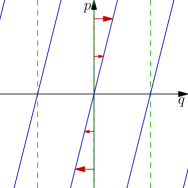
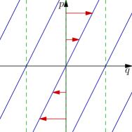
Figure 1. Shear transforms: dashed (green) vertical lines are transformed to solid (blue) slanted ones. An interpretation as a dynamics of a free particle: the momentum is constant, the coordinate is changed by an amount proportional to the momentum (cf. different arrows on the same picture) and the elapsed time (cf. the left and right pictures).

The geometrical meaning of this transformation is shear transform with the angle $\tan^{-1}x_{2}$, see Fig. 1:

(2.13) $$n(x_{2})(x_{1},x_{3}):=\begin{pmatrix}1&0\\ -x_{2}&1\end{pmatrix}\begin{pmatrix}x_{1}\\ x_{3}\end{pmatrix}=\begin{pmatrix}x_{1}\\ -x_{2}x_{1}+x_{3}\end{pmatrix}.$$

Note, that this also describes a physical picture for a particle with coordinate $x_{3}$ and the constant velocity $x_{1}$: after a period of time $-x_{2}$ the particle will still have the velocity $x_{1}$ but its new coordinate will be $x_{3}-x_{2}x_{1}$. We shall refer to both geometric and physical interpretation of the shear transform in § 4.2 in connection with the dynamic of the harmonic oscillator.

Another important group of symplectomorphisms—squeezing—are produced by matrices $\begin{pmatrix}a&0\\ 0&a^{-1}\end{pmatrix}\in\mathrm{SL}_{2}(\mathbb{R}{})$. These transformations act transitively on the set of minimal uncertainty states $\phi$, such that $\Delta_{\phi}Q\cdot\Delta_{\phi}P=\frac{\hslash}{2}$—the minimal value admitted by the Heisenberg–Kennard uncertainity relation [Folland89]*§ 1.3.

A related origin of the group $\mathbb{G}{}$ is the universal enveloping algebra $\mathcal{H}$ of $\mathfrak{h}$ spanned by elements $Q$, $P$ and $I$ with $[P,Q]=I$. It is known that the Lie algebra of Schrödinger group can be identified with the subalgebra spanned by the elements $\{Q,P,I,Q^{2},P^{2},\frac{1}{2}(QP+PQ)\}\subset\mathcal{H}$. This algebra is known as quadratic algebra in quantum mechanics [Gazeau09a]*§ 2.2.4. From the above discussion of the Schrödinger group, the identification

$$X_{1}\mapsto P,\quad X_{2}\mapsto\textstyle\frac{1}{2}Q^{2},\quad X_{3}\mapsto Q,\quad X_{4}\mapsto I$$

embeds the Lie algebra $\mathfrak{g}$ into $\mathcal{H}$. In particular, the identification $X_{2}\mapsto\textstyle\frac{1}{2}Q^{2}$ was used in physical literature to treat anharmonic oscillator with quartic potential [AllenAnastassiouKlink97, Klink94, JorgensenKlink85]. Furthermore, the group $\mathbb{G}{}$ is isomorphic to the Galilei group via the identification of respective Lie algebras

$$X_{1}\mapsto-Q,\quad X_{2}\mapsto\textstyle\frac{1}{2}P^{2},\quad X_{3}\mapsto P,\quad X_{4}\mapsto I.$$

That is, both algebras are related by Fourier transform.

We shall note that consideration of $\mathbb{G}{}$ as a subgroup of the Schrödinger group or the universal enveloping algebra $\mathcal{H}$ has a limited scope since only representations ${\rho_{h_{2}\hslash_{4}}}$ with $h_{2}=0$ appear as restrictions of representations of Schrödinger group, see [deGosson11a]*Ch. 7 [deGosson06a]*Ch. 7 [Folland89]*§ 4.2.

3. The induced coherent state transform and its image

We consider here the transformation which plays the crucial role in geometrisation of many concepts. If this transformation is reduced from the group $\mathbb{G}{}$ to the Heisenberg group it coincides with the Fock–Segal–Bargmann transform.

3.1. Induced coherent state transform of the group $\mathbb{G}{}$

Let $G$ be a Lie group with a left Haar measure $\mathrm{d}g$ and ${\rho}$ a unitary irreducible representation UIR of the group $G$ in a Hilbert space $\mathsf{H}{}$. Then, we define the coherent state transform as follows

Definition 3.1.

[AliAntGaz14a, Kisil11c] For a fixed vector $\phi\in\mathsf{H}{},$ called a fiducial vector (aka vacuum vector, ground state, mother wavelet), the coherent state transform, denoted $\mathcal{W}_{\phi}^{{\rho}}$ (or just $\mathcal{W}_{\phi}$ when it is clear from the context), of a vector $f\in\mathsf{H}{}$ is given by:

$$[\mathcal{W}_{\phi}^{{\rho}}f](g)=\left\langle{\rho}(g^{-1})f,\phi\right\rangle=\left\langle f,{\rho}(g)\phi\right\rangle,\qquad g\in G.$$

Let a fiducial vector $\phi$ be a joint eigenvector of ${\rho}(h)$ for all $h$ in a subgroup $H$, that is

(3.1) $${\rho}(h)\phi=\chi(h)\phi\quad\text{for all}\quad h\in H,$$

where $\chi$ is a character of $H$. Then, straightforward transformations show that [Kisil11c]*§ 5.1 [Kisil17a]*§ 5.1:

(3.2) $$[\mathcal{W}_{\phi}^{{\rho}}f](gh) =\overline{\chi}(h)[\mathcal{W}_{\phi}^{{\rho}}f](g).$$

This, in turn, indicates that the coherent state transform is entirely defined via its values indexed by points of $X=G/H$. This motivates the following definition of the coherent state transform on the homogeneous space $X=G/H:$

Definition 3.2.

For a group $G$, its subgroup $H$, a section $\mathsf{s}:G/H\rightarrow G$, UIR ${\rho}$ of $G$ in a Hilbert space $\mathsf{H}{}$ and a vacuum vector $\phi$ satisfying (3.1), we define the induced coherent state transform $\mathcal{W}_{\phi}^{{\rho}}$ from $\mathsf{H}{}$ to a space of function $\mathsf{L}_{\phi}{}(G/H)$ by the formula

(3.3) $$[\mathcal{W}_{\phi}^{{\rho}}f](x)=\langle f,{\rho}(\mathsf{s}(x))\phi\rangle,\qquad x\in G/H\,.$$

Proposition 3.3.

[Kisil11c]*§ 5.1 [Kisil17a]*§ 5.1 Let $G$, $H$, ${\rho}$, $\phi$ and $\mathcal{W}_{\phi}^{{\rho}}$ be as in Definition 3.2 and $\chi$ be a character from (3.1). Then the induced coherent state transform intertwines ${\rho}$ and $\tilde{{\rho}}$

(3.4) $$\mathcal{W}^{{\rho}}_{\phi}{\rho}(g)=\tilde{{\rho}}(g)\mathcal{W}^{{\rho}}_{\phi},$$

where $\tilde{{\rho}}$ is an induced representation from the character $\chi$ of the subgroup $H$.

In particular, (3.4) means that the image space $\mathsf{L}_{\phi}{}(G/H)$ of the induced coherent state transform is invariant under $\tilde{{\rho}}$.

For the subgroup $H$ being the centre $Z=\{(0,0,0,x_{4})\in\mathbb{G}{}:x_{4}\in\mathbb{R}{}\}$ of $\mathbb{G}{}$, the representation ${\rho_{h_{2}\hslash_{4}}}$ (2.6) and the character $\chi(0,0,0,x_{4})=\mathrm{e}^{2\pi\mathrm{i}\hslash_{4}x_{4}}$ any function $\phi\in\mathsf{L}_{2}{}(\mathbb{R}{})$ satisfies the eigenvector property (3.1). Thus, for the respective homogeneous space $\mathbb{G}{}/Z\sim\mathbb{R}^{3}{}$ and the section $\mathsf{s}:\mathbb{G}{}/Z\to\mathbb{G}{};\ \mathsf{s}(x_{1},x_{2},x_{3})=(x_{1},x_{2},x_{3},0)$ the induced coherent state transform is:

$$[\mathcal{W}_{\phi}f](x_{1},x_{2},x_{3}) =\langle f,{\rho_{h_{2}\hslash_{4}}}(\mathsf{s}(x_{1},x_{2},x_{3}))\phi\rangle$$

$$=\langle f,{\rho_{h_{2}\hslash_{4}}}(x_{1},x_{2},x_{3},0)\phi\rangle$$

$$=\int_{\mathbb{R}{}}f(y)\,\overline{{\rho_{h_{2}\hslash_{4}}}(x_{1},x_{2},x_{3},0)\,\phi(y)}\,\mathrm{d}y$$

$$=\int_{\mathbb{R}{}}f(y)\,\mathrm{e}^{-2\pi\mathrm{i}(h_{2}x_{2}+\hslash_{4}(-x_{3}y+\frac{1}{2}x_{2}y^{2}))}\,\overline{\phi}(y-x_{1})\,\mathrm{d}y$$

(3.5) $$=\mathrm{e}^{-2\pi\mathrm{i}h_{2}x_{2}}\int_{\mathbb{R}{}}f(y)\,\mathrm{e}^{-2\pi\mathrm{i}\hslash_{4}(-x_{3}y+\frac{1}{2}x_{2}y^{2})}\,\overline{\phi}(y-x_{1})\,\mathrm{d}y.$$

The last integral is a composition of the following three unitary operators of $\mathsf{L}_{2}{}(\mathbb{R}^{2}{})$:

1. The measure-preserving change of variables

   (3.6) $$T:F(x_{1},y)\mapsto F(y,y-x_{1})\,,$$

   where $F(x_{1},y):=(f\otimes\overline{\phi})(x_{1},y)=f(x_{1})\overline{\phi}(y)$, that is, $F$ is defined on the tenser product $\mathsf{L}_{2}{}(\mathbb{R}{})\otimes\mathsf{L}_{2}{}(\mathbb{R}{})$ which is isomorphic to $\mathsf{L}_{2}{}(\mathbb{R}^{2}{})$;

2. the operator of multiplication by an unimodular function $\psi_{x_{2}}(x_{1},y)=\mathrm{e}^{-\pi{\mathrm{i}}\hslash_{4}x_{2}y^{2}}$

   (3.7) $$M_{x_{2}}:F(x_{1},y)\mapsto\mathrm{e}^{-\pi{\mathrm{i}}\hslash_{4}x_{2}y^{2}}F(x_{1},y),\quad x_{2}\in\mathbb{R}{};$$

3. and the partial inverse Fourier transform in the second variable

   (3.8) $$[\mathcal{F}_{2}F](x_{1},x_{3})=\int_{\mathbb{R}{}}F(x_{1},y)\mathrm{e}^{2\pi\mathrm{i}\hslash_{4}yx_{3}}\,\mathrm{d}y.$$

Thus, [$\mathcal{W}_{\phi}f](x_{1},x_{2},x_{3})=\mathrm{e}^{-2\pi\mathrm{i}h_{2}x_{2}}[\mathcal{F}_{2}\circ M_{x_{2}}\circ T]F(x_{1},x_{3})$ and we obtain

Proposition 3.4.

For a fixed $x_{2}\in\mathbb{R}{}$, the map $f\otimes\overline{\phi}\mapsto[\mathcal{W}_{\phi}f](\cdot,x_{2},\cdot)$ is a unitary operator on $\mathsf{L}_{2}{}(\mathbb{R}^{2}{})$.

Such an induced coherent state transform also respects the Schwartz space, that is, if $f,\phi\in\mathsf{S}{}(\mathbb{R}{})$ then $[\mathcal{W}_{\phi}f](\cdot,x_{2},\cdot)\in\mathsf{S}{}(\mathbb{R}^{2}{})$. This is because $\mathsf{S}{}(\mathbb{R}^{2}{})$ is invariant under each operator (3.6)–(3.8).

Remark 3.5.

It is known fact [CorwinGreenleaf90a]*§ 4.5 that the coherent state transform on a nilpotent Lie group, cf. Definition 3.1, does not produce an $\mathsf{L}_{2}{}$-function on the entire group but may rather do on a certain homogeneous space. The leading example is the Heisenberg group when considering the homogeneous space $\mathbb{H}{}/Z$. In the context of coherent state transform, two types of modified square-integrability are considered [CorwinGreenleaf90a]*§ 4.5: modulo the group’s center and modulo the kernel of the representation. The first notion is not applicable to the group $\mathbb{G}{}$: the coherent state transform (3.5) does not define a square-integrable function on $\mathbb{G}{}/Z\sim\mathbb{R}^{3}{}$ or a larger space $\mathbb{G}{}/\mathrm{ker}{\rho_{h_{2}\hslash_{4}}}$. On the other hand, the representation ${\rho_{h_{2}\hslash_{4}}}$ is square-integrable modulo the subgroup $H=\{(0,x_{2},0,x_{4})\in\mathbb{G}{}:x_{2},x_{4}\in\mathbb{R}{}\}$. However, the theory of $\alpha$-admissibility [AliAntGaz14a]*§ 8.4, which is supposed to work for such cases, reduces the consideration to the Heisenberg group since $\mathbb{G}{}/H\sim\mathbb{H}{}/Z$. It shall be seen later (4.13) that the action of $(0,x_{2},0,0)\in H$ will be involved in important physical and geometrical aspects of the state of the harmonic oscillator and shall not be factored out. Our study provides an example of the theory of wavelet transform with non-admissible mother wavelets [Kisil09d, Kisil10c, Kisil98a, Zimmermann06, Guerrero18].

In view of the mentioned above insufficiency of square integrability modulo the subgroup $H=\{(0,x_{2},0,x_{4})\in\mathbb{G}{}:x_{2},x_{4}\in\mathbb{R}{}\}$, we make the following

Definition 3.6.

For a fixed unit vector $\phi\in\mathsf{L}_{2}{}(\mathbb{R}{})$, let $\mathsf{L}_{\phi}{}(\mathbb{G}{}/Z)$ denote the image space of the coherent state transform $\mathcal{W}_{\phi}$ (3.5) equipped with the family of inner products parametrised by $x_{2}\in\mathbb{R}{}$

(3.9) $$\left\langle u,v\right\rangle_{x_{2}}:=\int_{\mathbb{R}^{2}{}}u(x_{1},x_{2},x_{3})\,\overline{v(x_{1},x_{2},x_{3})}\,\hslash_{4}\,\mathrm{d}{x_{1}}\mathrm{d}{x_{3}}\,.$$

The respective norm is denoted by $\left\|u\right\|_{x_{2}}$.

Remark 3.7.

In physical applications the elements $x_{1}$, $x_{2}$ and $x_{3}$ are physical quantities and shall have physical units, cf. the consideration in [Kisil02e, Kisil17a] for the Heisenberg group and quantization problem in general. Let $L$ denote the unit of length, $M$ that of mass and $T$ that of time. Then, $x_{1}$ has dimension $\frac{T}{ML}$ (reciprocal to momentum) and $x_{3}$ has dimension $1/L$ (reciprocal to position.) So, from (2.2) $x_{2}$ has dimension $\frac{M}{T}$. Also, $h_{2}$, the dual to $x_{2}$ has reciprocal dimension to $x_{2}$, that is, it has dimension $\frac{T}{M}$ as well as $\hslash_{4}$ has dimension $\frac{ML^{2}}{T}$ of action which is reciprocal to the dimension of the product $x_{1}x_{3}$ or $x_{4}$. Dimensionality of $\hslash_{4}$ coincides with that of Planck constant. Thus the factor $\hslash_{4}$ in the measure $\hslash_{4}\,\mathrm{d}{x_{1}}\mathrm{d}{x_{3}}$ makes it dimensionless, which is a natural physical requirement. Note also that the dimensionality of $\mathrm{d}{\rho^{X_{j}}}$ is reciprocal to that of $x_{j}.$

It follows from Prop. 3.4 that $\left\|u\right\|_{x_{2}}=\left\|u\right\|_{x^{\prime}_{2}}$ for any $x_{2}$, $x_{2}^{\prime}\in\mathbb{R}{}$ and $u\in\mathsf{L}_{\phi}{}(\mathbb{G}{}/Z)$. In the usual way [Folland89]*(1.42) the isometry from Prop. 3.4 implies the following orthogonality relation.

Corollary 3.8.

Let $f_{1}$, $f_{2}$, $\phi_{1}$, $\phi_{2}\in\mathsf{L}_{2}{}(\mathbb{R}{})$ then:

(3.10) $$\left\langle\mathcal{W}_{\phi_{1}}f_{1},\mathcal{W}_{\phi_{2}}f_{2}\right\rangle_{x_{2}}=\left\langle f_{1},f_{2}\right\rangle\overline{\left\langle\phi_{1},\phi_{2}\right\rangle}\qquad\text{ for any }x_{2}\in\mathbb{R}{}\,.$$

Corollary 3.9.

Let $\phi\in\mathsf{L}_{2}{}(\mathbb{R}{})$ have unit norm, then the coherent state transform $\mathcal{W}_{\phi}$ is an isometry with respect to the inner product (3.9).

Proof.

It is an immediate consequence of the previous corollary. Alternatively, for $f\in\mathsf{L}_{2}{}(\mathbb{R}{})$:

$$\left\|f\right\|_{\mathsf{L}_{2}{}(\mathbb{R}{})}=\left\|f\otimes\phi\right\|_{\mathsf{L}_{2}{}(\mathbb{R}^{2}{})}=\left\|\mathcal{W}_{\phi}f\right\|_{x_{2}}\,,$$

as follows from the isometry $\mathcal{W}_{\phi}:\mathsf{L}_{2}{}(\mathbb{R}{})\rightarrow\mathsf{L}_{2}{}(\mathbb{R}^{2}{})$ in Prop. 3.4. ∎

An inverse of the unitary operator $\mathcal{W}_{\phi}$ is given by its adjoint $\mathcal{M}_{\phi}(x_{2})=\mathcal{W}_{\phi}^{*}$ with respect to the inner product (3.9) parametrised by $x_{2}$:

(3.11) $$[\mathcal{M}_{\phi}(x_{2})f](t)=\int_{\mathbb{R}^{2}{}}f(x_{1},x_{2},x_{3}){\rho}(x_{1},x_{2},x_{3},0)\phi(t)\,\hslash_{4}\,\mathrm{d}x_{1}\,\mathrm{d}x_{3}.$$

More generally, for an analysing vector $\phi$ and a reconstructing vector $\psi$, for any $f$, $g\in\mathsf{L}_{2}{}(\mathbb{R}{})$ the orthogonality condition (3.10) implies:

$$\left\langle\mathcal{M}_{\psi}(x_{2})\circ\mathcal{W}_{\phi}f,g\right\rangle =\left\langle\mathcal{W}_{\phi}f,\mathcal{W}_{\psi}g\right\rangle_{x_{2}}$$

$$=\left\langle f,g\right\rangle\left\langle\psi,\phi\right\rangle\,.$$

Then $\mathcal{M}_{\psi}(x_{2})\circ\mathcal{W}_{\phi}=\left\langle\psi,\phi\right\rangle I$ and if $\left\langle\psi,\phi\right\rangle\neq 0$ then $\mathcal{M}_{\psi}(x_{2})$ is a left inverse of $\mathcal{W}_{\phi}$ up to a factor.

By Prop. 3.3 the transform $\mathcal{W}_{\phi}$ intertwines ${\rho_{h_{2}\hslash_{4}}}$ with the following representation on $\mathsf{L}_{2}{}(\mathbb{R}^{3}{})$ (see (2.5))

(3.12) $$[{\tilde{\rho}_{h_{4}}}(y_{1},y_{2},y_{3},y_{4})f](x_{1},x_{2},x_{3})=\mathrm{e}^{2\pi\mathrm{i}\hslash_{4}(y_{4}-y_{1}y_{3}+\frac{1}{2}y_{1}^{2}y_{2}+y_{1}x_{3}-\frac{1}{2}y_{1}^{2}x_{2})}\\ \times f(x_{1}-y_{1},x_{2}-y_{2},x_{3}-y_{1}x_{2}+y_{1}y_{2}-y_{3})\,.$$

We consider this representation restricted to the image space $\mathsf{L}_{\phi}{}(\mathbb{G}{}/Z)$, unitarity of ${\tilde{\rho}_{\hslash_{4}}}$ is easily seen.

3.2. Characterisation of the image space

The following result plays a fundamental role in exploring the nature of the image space of the coherent state transform and is a recurrent theme of our investigation, see also [Kisil11c]*§ 5[Kisil13c] [Kisil17a]*§ 5.3.

Corollary 3.10 (Analyticity of the coherent state transform, [Kisil11c]*§ 5).

Let $G$ be a group and $\mathrm{d}g$ be a measure on $G$. Let ${\rho}$ be a unitary representation of $G$, which can be extended by integration to a vector space $V$ of functions or distributions on $G$. Let a fiducial vector $\phi\in\mathsf{H}{}$ satisfy the equation

(3.13) $$\int_{G}d(g)\,{\rho}(g)\phi\,\mathrm{d}g=0,$$

for a fixed distribution $d(g)\in V$. Then, any coherent state transform $\tilde{v}(g)=\left\langle v,{\rho}(g)\phi\right\rangle$ obeys the condition:

(3.14) $$D\tilde{v}=0,\qquad\text{where}\quad D=\int_{G}\bar{d}(g)\,R(g)\,\mathrm{d}g\,,$$

with $R$ being the right regular representation of $G$ and $\bar{d}(g)$ is the complex conjugation of ${d}(g)$.

Example 3.11.

To describe the image space $\mathsf{L}_{\phi}{}(\mathbb{G}{}/Z)$ of the respective induced coherent state transform, we employ Corollary 3.10. This requires a particular choice of a fiducial vector $\phi$ such that $\phi$ lies in $\mathsf{L}_{2}{}(\mathbb{R}{})$ and $\phi$ is a null solution of an operator of the form (3.13). For simplicity, we consider the following first-order operator, which represents an element of the Lie algebra $\mathfrak{g}$, cf. (2.8):

$$\mathrm{d}{\rho^{\mathrm{i}X_{1}+\mathrm{i}aX_{2}+EX_{3}}_{h_{2}\hslash_{4}}} =\mathrm{i}\mathrm{d}{\rho^{X_{1}}_{h_{2}\hslash_{4}}}+\mathrm{i}a\,\mathrm{d}{\rho^{X_{2}}_{h_{2}\hslash_{4}}}+E\,\mathrm{d}{\rho^{X_{3}}_{h_{2}\hslash_{4}}}$$

(3.15) $$=-\mathrm{i}\frac{\mathrm{d}\ }{\mathrm{d}y}-\pi\hslash_{4}ay^{2}-2\pi\mathrm{i}E\hslash_{4}y-2\pi h_{2}a\,,$$

where $a$ and $E$ are some real constants. It is clear that, the function

(3.16) $$\phi(y)=c\exp\left(\frac{\pi\mathrm{i}a\hslash_{4}}{3}y^{3}-\pi E\hslash_{4}y^{2}+2\pi\mathrm{i}ah_{2}y\right),$$

is a generic solution of (3.15) where $c$ is an arbitrary constant determined by $\mathsf{L}{}_{2}$-normalisation while square integrability of $\phi$ requires that $E\hslash_{4}$ is strictly positive. Furthermore, it is sufficient for the purpose of this work to use the simpler fiducial vector corresponding to the value $a=0$, thus we set

(3.17) $$\phi(y)=c\,\mathrm{e}^{-\pi E\hslash_{4}y^{2}},\qquad\hslash_{4}>0,\ E>0.$$

Since the function $\phi(y)$ (3.17) is a null-solution of the operator (3.15) with $a=0$, the image space $\mathsf{L}_{\phi}{}(\mathbb{G}{}/Z)$ can be described through the respective derived right regular representation (Lie derivatives) (2.10). Specifically, Corollary 3.10 with the distribution

$$d(x_{1},x_{2},x_{3},x_{4})=\mathrm{i}\,\delta^{\prime}_{1}(x_{1},x_{2},x_{3},x_{4})+E\,\delta^{\prime}_{3}(x_{1},x_{2},x_{3},x_{4})\,,$$

where $\delta^{\prime}_{j}$ is the partial derivative of the Dirac delta distribution $\delta$ with respect to $x_{j}$, matches (3.15). Thus, any function $f$ in $\mathsf{L}_{\phi}{}(\mathbb{G}{}/Z)$ for $\phi$ (3.17) satisfies $\mathcal{C}f=0$ for the partial differential operator:

(3.18) $$\mathcal{C}=\left(-\mathrm{i}\mathfrak{L}^{X_{1}}+E\mathfrak{L}^{X_{3}}\right)=-\mathrm{i}\partial_{1}+E\partial_{3}-2\pi\mathrm{i}\hslash_{4}E{x_{1}}\,,$$

where Lie derivatives (2.11) are used.

Due to the explicit similarity to the Heisenberg group case with the Cauchy–Riemann equation, we call (3.18) the analyticity condition for the coherent state transform. Indeed, it can be easily verified that

$$[\mathcal{W}_{\phi}k](x_{1},x_{2},x_{3})=\exp(-2\pi\mathrm{i}h_{2}x_{2}+\pi{\mathrm{i}}\hslash_{4}x_{1}x_{3}-\frac{\pi\hslash_{4}}{2E}(E^{2}x_{1}^{2}+x_{3}^{2}))B_{x_{2}}(x_{1},x_{3})$$

where

$$B_{x_{2}}(x_{1},x_{3}) =\int_{\mathbb{R}}\mathrm{e}^{-\pi{\mathrm{i}}\hslash_{4}x_{2}y^{2}}k(y)\mathrm{e}^{\frac{\pi\hslash_{4}}{2E}(x_{3}-\mathrm{i}Ex_{1})^{2}+2\pi\mathrm{i}\hslash_{4}(x_{3}-\mathrm{i}Ex_{1})y-\pi\hslash_{4}Ey^{2}}\;\mathrm{d}y$$

$$=[(V_{E}\circ M_{x_{2}})k](x_{1},x_{3})$$

and $V_{E}$ is Fock–Segal–Bargmann type transform [Folland89, Kisil11c, Kirillov04a, Neretin11a] and $M_{x_{2}}$ is a multiplication operator by $\mathrm{e}^{-\pi\hslash_{4}x_{2}y^{2}}$. Thus, by condition (3.18) we have

$$[-\mathrm{i}\partial_{1}+E\partial_{3}$$

$$\quad-2\pi\mathrm{i}\hslash_{4}E{x_{1}}]\{\exp(-2\pi\mathrm{i}h_{2}x_{2}+\pi{\mathrm{i}}\hslash_{4}x_{1}x_{3}-\frac{\pi\hslash_{4}}{2E}(E^{2}x_{1}^{2}+x_{3}^{2}))B_{x_{2}}(x_{1},x_{3})\}=0.$$

That is,

(3.19) $$(-\mathrm{i}\partial_{1}+E\partial_{3})B_{x_{2}}(x_{1},x_{3})=0,$$

which can be written as

(3.20) $$\partial_{\overline{z}}B_{x_{2}}(z)=0,$$

where $z=x_{3}-\mathrm{i}Ex_{1}$ and $\partial_{\overline{z}}=\frac{1}{2}(\frac{-\mathrm{i}}{E}\partial_{1}+\partial_{3})$—a Cauchy–Riemann type operator. Thus, $B_{x_{2}}(z)$ is entire on the complex plane $\mathbb{C}{}$ parametrised by points $(x_{1},x_{3})$. As such, the coherent state transform gives rise to the space consisting of analytic functions $B_{x_{2}}(z)$ which are square-integrable with respect to the measure $\mathrm{e}^{-\frac{\pi\hslash_{4}}{E}\left|z\right|^{2}}\mathrm{d}z$.

A notable difference between the group $\mathbb{G}{}$ and the Heisenberg group is the presence of an additional second-order condition, which is satisfied by any function $f\in\mathsf{L}_{\phi}{}(\mathbb{G}{}/Z)$ for any fiducial vector $\phi$. Indeed, the specific structure of the representation (2.8) implies that any function $\phi$ satisfies the relation for the derived representation,

(3.21) $$\left((\mathrm{d}{\rho^{X_{3}}_{h_{2}\hslash_{4}}})^{2}-2\,\mathrm{d}{\rho^{X_{2}}_{h_{2}\hslash_{4}}}\mathrm{d}{\rho^{X_{4}}_{h_{2}\hslash_{4}}}-{8\pi^{2}h_{2}\hslash_{4}}I\right)\phi=0.$$

This can by verified by (2.8) directly, but a deeper insight follows from an interpretation of (3.21) as the statement that the Casimir operator $C=X_{3}^{2}-2X_{1}X_{2}$ acts on the irreducible component as multiplication by the scalar ${8\pi^{2}h_{2}\hslash_{4}}$. Also Casimir operator $C$ appears in the Kirillov orbit method [CorwinGreenleaf90a]*Ex. 3.3.9 [Kirillov04a]*§ 3.3.1 in the natural parametrisation of coadjoint orbits—the topic further developed in [AldayaNavarro-Salas91a, AldayaGuerrero01a].

From here we can proceed in either way:

1. Corollary 3.10 with the distribution

   $$d(x_{1},x_{2},x_{3},x_{4})=\delta_{33}^{(2)}(x_{1},x_{2},x_{3},x_{4})-2\,\delta^{\prime}_{1}(x_{1},x_{2},x_{3},x_{4})\cdot\delta^{\prime}_{2}(x_{1},x_{2},x_{3},x_{4})\,,$$

   asserts that the image $f\in\mathsf{L}_{\phi}{}(\mathbb{G}{}/Z)$ of the coherent state transform $\mathcal{W}_{\phi}$ is annihilated by the respective Lie derivatives operator $\mathcal{S}f=0$ where, cf. (2.11):

   (3.22) $$\mathcal{S} =(\mathfrak{L}^{X_{3}})^{2}-2\mathfrak{L}^{X_{2}}\mathfrak{L}^{X_{4}}-{8\pi^{2}h_{2}\hslash_{4}}I$$

   $$=\partial_{33}^{2}+{4\pi\mathrm{i}}\hslash_{4}\partial_{2}-8\pi^{2}h_{2}\hslash_{4}I\,.$$

2. The representation, cf. (2.7):

   (3.23) $$\mathrm{d}{\tilde{\rho}^{C}_{\hslash_{4}}}=(\mathrm{d}{\tilde{\rho}^{X_{3}}_{\hslash_{4}}})^{2}-\mathrm{d}{\tilde{\rho}^{X_{2}}_{\hslash_{4}}}\mathrm{d}{\tilde{\rho}^{X_{4}}_{\hslash_{4}}}$$

   of the Casimir operator $C$ takes the constant value ${8\pi^{2}h_{2}\hslash_{4}}$ on $\mathsf{L}_{\phi}{}(\mathbb{G}{}/Z)$. Note, that this produces exactly (3.22) because for the Casimir operator the left and the right actions coincide.

The relation (3.22) will be called the structural condition because it is determined by the structure of the Casimir operator. Note, that (3.22) is a Schrödinger equation of a free particle with the time-like parameter $x_{2}$. Thus, the structural condition is the quantised version of the classical dynamics (2.13) of a free particle represented by the shear transform, see the discussion of this after (2.13).

Summing up, the physical characterisation of the $\mathsf{L}_{\phi}{}(\mathbb{G}{}/Z)$ is as follows:

1. The restriction of a function $f\in\mathsf{L}_{\phi}{}(\mathbb{G}{}/Z)$ to the plane $x_{2}=0$ (a model of the phase space) coincides with the FSB image of the respective state,

2. The function $f$ is a continuation from the plane $x_{2}=0$ to $\mathbb{R}^{2}{}\times\mathbb{R}{}$ (the product of phase space and timeline) by free time-evolution of the quantum system.

This physical interpretation once more explains the identity $\left\|f\right\|_{x_{2}}=\left\|f\right\|_{x^{\prime}_{2}}$: the energy of a free state is constant in time.

Summarising analysis in this subsection we specify the ground states and the respective coherent state transforms, which will be used below.

Example 3.12.

Consider our normalised fiducial vector $\phi_{E}(y)=({2h_{2}E})^{1/4}\mathrm{e}^{-\pi\hslash_{4}Ey^{2}}$ with a parameter $E>0$. It is normalised with respect to the norm $\left\|f\right\|^{2}=\int_{\mathbb{R}{}}\left|f(y)\right|^{2}\sqrt{\frac{\hslash_{4}}{h_{2}}}\;\mathrm{d}y$. Note, that for $\phi_{E}(y)$ to be dimensionless, $E$ has to be of dimension $M/T$, this follows from the fact that $y$ has dimension $T/ML$, thus for this reason we attach the factor $\sqrt{\frac{\hslash_{4}}{h_{2}}}$ to the measure so the measure is dimensionless. Then we calculate the coherent state transform of a minimal uncertainty state $\phi_{q}(y)$ ($q>0$) as follows:

$$[\mathcal{W}_{\phi_{E}}\phi_{q}](x_{1},x_{2},x_{3}) =\sqrt{2\hslash_{4}}(qE)^{1/4}\int_{\mathbb{R}}\mathrm{e}^{-\pi\hslash_{4}qy^{2}}\mathrm{e}^{-2\pi\mathrm{i}(h_{2}x_{2}+\hslash_{4}(-x_{3}y+\frac{1}{2}x_{2}y^{2}))}$$

$$\qquad\times\mathrm{e}^{-\pi\hslash_{4}E(y-x_{1})^{2}}\;\mathrm{d}y$$

$$=\sqrt{2\hslash_{4}}(qE)^{1/4}\mathrm{e}^{-\pi\hslash_{4}Ex_{1}^{2}-2\pi\mathrm{i}h_{2}x_{2}}\int_{\mathbb{R}}\mathrm{e}^{-\pi\hslash_{4}(\mathrm{i}x_{2}+E+q)y^{2}}$$

$$\qquad\times\mathrm{e}^{2\pi\hslash_{4}(Ex_{1}+\mathrm{i}x_{3})y}\;\mathrm{d}y$$

(3.24) $$={\sqrt{2}(qE)^{1/4}}\frac{\exp\left(-\pi h_{4}Ex_{1}^{2}-2\pi\mathrm{i}h_{2}x_{2}-\pi\hslash_{4}\frac{(-\mathrm{i}Ex_{1}+x_{3})^{2}}{\mathrm{i}x_{2}+E+q}\right)}{\sqrt{\mathrm{i}x_{2}+E+q}}.$$

Clearly, the function (3.24) is dimensionless and satisfies conditions (3.18) and (3.22). It shall be seen later that such a function is an eigenstate (vacuum state) of the harmonic oscillator Hamiltonian acting on the image space $\mathsf{L}_{\phi}{}(\mathbb{G}{}/Z)$ of the respective induced coherent state transform. Moreover, this function represents a minimal uncertinity state in the space $\mathsf{L}_{\phi}{}(\mathbb{G}{}/Z)$ for any $x_{2}\in\mathbb{R}$ and any $E>0$.

4. Harmonic oscillator through reduction of order of a PDE

Here we systematically treat the harmonic oscillator with the method of reducing PDE order for geometrisation of the dynamics. First we use the Heisenberg group and find that geometrisation condition completely determines which fiducial vector needs to be used. The treatment of the group $\mathbb{G}{}$ provides the wider opportunity: any minimal uncertainty state can be used for the coherent state transform with geometric dynamic in the result. In the next section we provide eigenfunctions and respective ladder operators.

4.1. Harmonic oscillator from the Heisenberg group

Here we use a simpler case of the Heisenberg group to illustrate the technique which will be used later. The fundamental importance of the harmonic oscillator stimulates exploration of different approaches. Analysis based on the pair of ladder operators elegantly produces the spectrum and the eigenvectors. However, this technique is essentially based on a particular structure of the Hamiltonian of harmonic oscillator expressed in terms of the Weyl Lie algebra. Thus, it loses its efficiency in other cases. In contrast, our method is applicable for a large family of examples since it has a more general nature.

The harmonic oscillator with constant mass $m$ and frequency $\omega$ has the classic Hamiltonian $\frac{1}{2}(p^{2}/m+m\omega^{2}q^{2})$. Its Fock–Segal–Bargmann quantisation, denoted by $H$, acts on $\mathsf{L}_{\phi}{}(\mathbb{H}{}/Z)$ parametrised by points $(x_{1},x_{3})$ and is given by

(4.1) $$Hf(x_{1},x_{3}) =\left(\frac{1}{2m}\left(\frac{\mathrm{i}\mathrm{d}\tilde{\sigma}_{\hslash}^{X_{1}}}{\sqrt{2\pi}}\right)^{2}+\frac{m\omega^{2}}{2}\left(\frac{\mathrm{i}\mathrm{d}\tilde{\sigma}_{\hslash}^{X_{3}}}{\sqrt{2\pi}}\right)^{2}\right)f(x_{1},x_{3})$$

$$=-\frac{1}{4\pi m}\partial_{11}^{2}(f)(x_{1},x_{3})-\frac{m\omega^{2}}{4\pi}\partial_{33}^{2}(f)(x_{1},x_{3})$$

$$\quad+\frac{\mathrm{i}\hslash}{m}x_{3}\partial_{1}(f)(x_{1},x_{3})+\frac{\pi\hslash^{2}}{m}x_{3}^{2}f(x_{1},x_{3}).$$

The time evolution of the harmonic oscillator is defined by the the Schrödinger equation for Hamiltonian $H;$

(4.2) $${\mathrm{i}\hslash}\partial_{t}f(t;x_{1},x_{3})-Hf(t;x_{1},x_{3})=0$$

for $f(0,x_{1},x_{3})$ in $\mathsf{L}_{\phi}{}(\mathbb{H}{}/Z)$. As was mentioned, the creation-annihilation pair produces spectral decomposition of $H$. Our aim is to describe dynamics of an arbitrary observable in geometric terms by lowering the order of the differential operator (4.1).

Indeed, the structure of $\mathsf{L}_{\phi}{}(\mathbb{H}{}/Z)$ enables to make a reduction to the order of equation (4.1) using the analyticity condition. For Gaussian $\phi(y)=\mathrm{e}^{-\pi\hslash Ey^{2}}$ ($E>0$) we have (the annihilation operator)

$$\mathrm{i}\mathrm{d}{\sigma_{\hslash}^{X_{1}}}\phi(y)+E\mathrm{d}{\sigma_{\hslash}^{X_{3}}}\phi(y)=0.$$

So, the respective image of induced coherent state transform, $f(x_{1},x_{3})=[\mathcal{W}^{\sigma_{\hslash}}_{\phi}k](x_{1},x_{3})$ for $k\in\mathsf{L}_{2}{}(\mathbb{R}{})$, is annihilated by the operator (the analyticity condition):

(4.3) $$\mathcal{D} =-\mathrm{i}\mathfrak{L}^{X_{1}}+E\mathfrak{L}^{X_{3}}$$

$$=-\mathrm{i}\partial_{1}+E\partial_{3}-2\pi\mathrm{i}\hslash Ex_{1}I\,,$$

we still write $f(0,x_{1},x_{3})$ as $f(x_{1},x_{3})$. From the analyticity condition (4.3) for induced coherent state transform, operator $(A\partial_{1}+\mathrm{i}B\partial_{3}+CI)(-\mathrm{i}\mathfrak{L}^{X_{1}}+E\mathfrak{L}^{X_{3}})$ vanishes on any $f\in\mathsf{L}_{\phi}{}(\mathbb{H}{}/Z)$ for any $A$, $B$ and $C$. Thus, we can adjust the Hamiltonian (4.1) by adding such a term

$$\tilde{H} =H+(A\partial_{1}+\mathrm{i}B\partial_{3}+CI)(-\mathrm{i}\mathfrak{L}^{X_{1}}+E\mathfrak{L}^{x_{3}})$$

through which $A,B$ and $C$ to be determined to eliminate the second-order derivatives in $\tilde{H}$. Thus it will be a first-order differential operator equal to $H$ on $\mathsf{L}_{\phi}{}(\mathbb{H}{}/Z)$. To achieve this we need to take $A=\frac{\mathrm{i}}{4\pi m}$, $B=-\frac{\mathrm{i}}{4\pi}\omega$, for $E=m\omega$. Note, that the value of $E$ is uniquely defined and consequently the corresponding vacuum vector $\phi(y)=\mathrm{e}^{-\pi\hslash Ey^{2}}$ is fixed. Furthermore, to obtain a geometric action of $\tilde{H}$ in the Schrödinger equation we need pure imaginary coefficients of the first-order derivatives in $\tilde{H}$. Thus, this produces $C=-\frac{\mathrm{i}\hslash\omega}{2}x_{1}$, with the final result:

$$\tilde{H} =\left(\frac{1}{2m}\left(\frac{\mathrm{i}\mathrm{d}\tilde{\sigma}_{\hslash}^{X_{1}}}{\sqrt{2\pi}}\right)^{2}+\frac{m\omega^{2}}{2}\left(\frac{\mathrm{i}\mathrm{d}\tilde{\sigma}_{\hslash}^{X_{3}}}{\sqrt{2\pi}}\right)^{2}\right)$$

$$\quad+(\frac{\mathrm{i}}{4\pi m}\partial_{1}+\frac{\omega}{4\pi}\partial_{3}-\frac{\mathrm{i}\hslash\omega}{2}x_{1}I)(-\mathrm{i}\mathfrak{L}^{X_{1}}+m\omega\mathfrak{L}^{X_{3}})$$

(4.4) $$=\frac{\mathrm{i}\hslash}{m}x_{3}\partial_{1}-\mathrm{i}\hslash m\omega^{2}x_{1}\partial_{3}+\left(\frac{1}{2}\hslash\omega+\frac{\pi\hslash^{2}}{m}(x_{3}^{2}-m^{2}\omega^{2}x_{1}^{2})\right)I\,.$$

Note, that operators (4.1) and (4.4) are not equal in general but have the same restriction to the kernel of the auxiliary analytic condition (4.3). Thus, we aim to find a solution to (4.2), with $\tilde{H}$ (4.4) in place of $H$ on the space of functions that satisfies the analyticity condition (4.3). Since the operator in (4.3) (for $E=m\omega$) is intertwined with the Cauchy–Riemann type operator by operator of multiplication by $\mathrm{e}^{-\pi\hslash m\omega x_{1}^{2}}$, the generic solution of (4.3) is

(4.5) $$f(x_{1},x_{3})=\mathrm{e}^{-\pi\hslash m\omega x_{1}^{2}}f_{1}\left(x_{3}-\mathrm{i}m\omega x_{1}\right)\,,$$

where $f_{1}(z)$ is an analytic function of one complex variable. Then, we use the method of characteristics to solve the first-order PDE (4.2) with $\tilde{H}$ (4.4) for the function $f(x_{1},x_{3})$ (4.5) to obtain the solution:

(4.6) $$f(t;x_{1},x_{3})=\exp\left(\frac{-\mathrm{i}\omega}{2}t+\pi{\mathrm{i}}\hslash x_{1}x_{3}-\frac{\pi\hslash}{2m\omega}(m^{2}\omega^{2}x_{1}^{2}+x_{3}^{2})\right)f_{2}\left(\mathrm{e}^{-\mathrm{i}\omega t}(x_{3}-\mathrm{i}m\omega x_{1})\right)$$

where for $t=0$ the solution formula (4.6) is a particular case of (4.5) with $f_{1}(z)=\mathrm{e}^{-\frac{\pi\hslash}{2m\omega}z^{2}}f_{2}(z)$ so it satisfies the analyticity condition (4.3). Thus, formula (4.6) also satisfies (4.2) with the proper harmonic oscillator Hamiltonian (4.1). It is well known that this solution geometrically corresponds to a uniform rotation of the phase space.

4.2. Harmonic oscillator from the group $\mathbb{G}{}$

Here we obtain an exact solution of the harmonic oscillator in the space $\mathsf{L}_{\phi}{}(\mathbb{G}{}/Z)$. It is fulfilled by the reduction of the order of the corresponding differential operator in a manner illustrated on the Heisenberg group in Section 4.1. A new feature of this case is that we need to use both operators (3.18) and (3.22) simultaneously.

The Weyl quantisation of the harmonic oscillator Hamiltonian $\frac{1}{2}(p^{2}/m+m\omega^{2}q^{2})$ is given by:

$$H =\left(\frac{1}{2m}\left(\frac{\mathrm{i}\mathrm{d}{\tilde{\rho}^{X_{1}}_{\hslash_{4}}}}{\sqrt{2\pi}}\right)^{2}+\frac{m\omega^{2}}{2}\left(\frac{\mathrm{i}\mathrm{d}{\tilde{\rho}^{X_{3}}_{\hslash_{4}}}}{\sqrt{2\pi}}\right)^{2}\right)$$

(4.7) $$=-\frac{1}{4\pi m}\partial_{11}^{2}-\frac{1}{4\pi m}x_{2}^{2}\partial_{33}^{2}-\frac{m\omega^{2}}{4\pi}\partial_{33}^{2}-\frac{1}{2\pi m}x_{2}\partial_{13}^{2}$$

$$\quad+\frac{\mathrm{i}\hslash_{4}}{m}x_{3}\partial_{1}+\frac{\mathrm{i}\hslash_{4}}{m}x_{2}x_{3}\partial_{3}-\frac{1}{2m}(-\mathrm{i}\hslash_{4}x_{2}-2\pi\hslash_{4}^{2}x_{3}^{2})I\,.$$

Although, the Hamiltonian seems a bit alienated in comparison with the Heisenberg group case, cf. (2.7), we can still adjust it by using conditions (3.18) and (3.22) as follows:

(4.8) $$H_{1}=H+(A\partial_{1}+B\partial_{2}+C\partial_{3}+KI)\mathcal{C}+F\mathcal{S}\,.$$

To eliminate all second order derivatives one has to take $A=\frac{\mathrm{i}}{4\pi m}$, $B=0$, $C=\frac{\mathrm{i}}{2\pi m}(\frac{-\mathrm{i}}{2}E+x_{2})$ and $F=-\frac{1}{4\pi m}(\mathrm{i}x_{2}+E)^{2}+\frac{m\omega^{2}}{4\pi}$. A significant difference from the Heisenberg group case is that there is no particular restrictions for the parameter $E$. This allows to use functions $\mathrm{e}^{-\pi\hslash_{4}Ey^{2}}$, with any $E>0$ as fiducial vectors. Such functions are known as squeezed (or two-photon [Yuen76]) states and play an important role in quantum theory, see original papers [WodkiewiczEberly85, Wodkiewicz87, Walls83, Stoler70, deGosson13a] and textbooks [Walls08]*§ 2.4–2.5 [Schleich01a]*§ 4.3 [Gazeau09a]*Ch. 10 [deGosson11a]*§ 11.3.

To make the action of the first order operator geometric we make coefficients in front of the first-order derivatives $\partial_{1}$ and $\partial_{3}$ imaginary. For this we put $K=\frac{\mathrm{i}\hslash_{4}}{2m}x_{1}(-E+2\mathrm{i}x_{2})$. The final result is:

(4.9) $$H_{1} ={H+(\frac{1}{4\pi m}(x_{2}+\mathrm{i}E)^{2}+\frac{m\omega^{2}}{4\pi})\mathcal{S}}\quad$$

$$\quad+\left(\frac{\mathrm{i}}{4\pi m}\partial_{1}+\frac{\mathrm{i}}{2\pi m}(\frac{-\mathrm{i}}{2}E+x_{2})\partial_{3}+\frac{\mathrm{i}\hslash_{4}}{2m}x_{1}(-E+2\mathrm{i}x_{2})\right)\left(-\mathrm{i}\mathfrak{L}^{X_{1}}+E\mathfrak{L}^{X_{3}}\right)$$

$$=\frac{\mathrm{i}\hslash_{4}}{m}\left((x_{3}+x_{1}x_{2})\partial_{1}-\left((\mathrm{i}x_{2}+E)^{2}-m^{2}\omega^{2}\right)\partial_{2}-(E^{2}x_{1}-x_{2}x_{3})\partial_{3}\right)$$

$$\quad-\frac{\hslash_{4}}{2m}\left(-8\mathrm{i}\pi h_{2}Ex_{2}-{\mathrm{i}}x_{2}+4\pi h_{2}x_{2}^{2}-2\pi\hslash_{4}x_{3}^{2}\right.$$

$$\qquad\left.+4\pi h_{2}m^{2}\omega^{2}-E-4\pi h_{2}E^{2}-{4\mathrm{i}}\pi E\hslash_{4}x_{1}^{2}x_{2}+2\pi\hslash_{4}E^{2}x_{1}^{2}\right)I\,.$$

Thus, the Schrödinger equation for the harmonic oscillator

(4.10) $$\mathrm{i}\hslash_{4}\partial_{t}f(t;x_{1},x_{2},x_{3})-Hf(t;x_{1},x_{2},x_{3})=0,$$

is equivalent to the first order linear PDE

(4.11) $$\mathrm{i}\hslash_{4}\partial_{t}f(t;x_{1},x_{2},x_{3})-H_{1}f(t;x_{1},x_{2},x_{3})=0,$$

for $f$ in the image space $\mathsf{L}_{\phi}{}(\mathbb{G}{}/Z)$. It can be solved by the following steps:

1. We start by peeling the analytic operator (3.18) into a Cauchy–Riemann type operator. Indeed, the operator of multiplication

   $$\mathcal{G}:f(x_{1},x_{2},x_{3})\mapsto\mathrm{e}^{-\pi\hslash_{4}Ex_{1}^{2}}f(x_{1},x_{2},x_{3})$$

   intertwines the analytic operator (3.18)—the Cauchy–Riemann type operator:

   $$\mathcal{G}\circ\mathcal{C}=(E\partial_{3}-\mathrm{i}\partial_{1})\circ\mathcal{G}.$$

   Thus, a generic solution of the analytic condition $\mathcal{C}f(x_{1},x_{2},x_{3})=0$ has the form:

   (4.12) $$f(x_{1},x_{2},x_{3})=\mathrm{e}^{-\pi\hslash_{4}Ex_{1}^{2}}f_{1}(x_{3}-\mathrm{i}Ex_{1},\mathrm{i}x_{2}+E),$$

   where $f_{1}$ is an arbitrary analytic function of two complex variables.

2. Subsequently, the first order PDE (4.11) for the function $f(x_{1},x_{2},x_{3})$ (4.12) has, by the standard method of characteristics, the following general solution:

   (4.13) $$\begin{split}f(t;x_{1},x_{2},x_{3})&=\,\frac{\sqrt{E+m\omega}}{\sqrt{\mathrm{i}x_{2}+E+m\omega}}\\ &\quad\times\exp\left(\frac{-\mathrm{i}\omega}{2}t-\pi{\hslash_{4}}Ex_{1}^{2}-2\pi\mathrm{i}h_{2}x_{2}-\pi{\hslash_{4}}\frac{(x_{3}-\mathrm{i}Ex_{1})^{2}}{\mathrm{i}x_{2}+E+m\omega}\right)\\ &\quad\times f_{2}\left(\mathrm{e}^{-\mathrm{i}\omega t}\frac{x_{3}-\mathrm{i}Ex_{1}}{\mathrm{i}x_{2}+E+m\omega},\mathrm{e}^{-2\mathrm{i}\omega t}\frac{m\omega-(\mathrm{i}x_{2}+E)}{m\omega+(\mathrm{i}x_{2}+E)}\right).\end{split}$$

   This is a particular case of formula  (4.12) for $t=0$ and

   $$f_{1}(y_{1},y_{2})=\frac{\sqrt{E+m\omega}\exp\left(2\pi\mathrm{i}h_{2}(E-y_{2})-\frac{\pi\hslash_{4}y_{1}^{2}}{y_{2}+m\omega}\right)}{\sqrt{y_{2}+m\omega}}f_{2}\left(\frac{y_{1}}{y_{2}+m\omega},\frac{m\omega-y_{2}}{m\omega+y_{2}}\right)$$

   here  $y_{1}=x_{3}-\mathrm{i}Ex_{1}$ and  $y_{2}=\mathrm{i}x_{2}+E$ and $f_{2}$ is an arbitrary analytic function of two complex variables. Hence, (4.13) satisfies the analyticity condition (3.18). It also satisfies (4.11) with the reduced Hamiltonian (4.9), yet, it is not a solution to (4.10) with the original Hamiltonian (4.7).

3. In the final step we request that (4.13) satisfy the structural condition (3.22). This results in a heat-like equation in terms of $f_{2}$:

   (4.14) $$\partial_{u}f_{2}(z,u)=-\frac{1}{8\pi\hslash_{4}m\omega}\partial^{2}_{zz}f_{2}(z,u)$$

   where

   $$z=\frac{x_{3}-\mathrm{i}Ex_{1}}{\mathrm{i}x_{2}+E+m\omega}\,,\quad u=\frac{m\omega-(\mathrm{i}x_{2}+E)}{m\omega+(\mathrm{i}x_{2}+E)}\,.$$

   The well-known fundamental solution of (4.14) is:

   (4.15) $$f_{2}(z,u)=\left(\frac{2m\omega\hslash_{4}}{u}\right)^{1/2}\int_{\mathbb{R}{}}g(\xi)\,\mathrm{e}^{2\pi\hslash_{4}m\omega\frac{(z-\xi)^{2}}{u}}\,\mathrm{d}\xi,$$

   where $g$ is the initial condition $g(z)=f_{2}(z,0)$ and we use analytic extension from the real variable $u$ to some neighbourhood of the origin in the complex plane—see discussion in § 4.3. Thus, with $f_{2}$ as in (4.15), formula (4.13) yields a generic solution to (4.10) with Hamiltonian (4.7).

Remark 4.1.

Note that the above initial value of $f_{2}$, related to $u=0$, corresponds to $x_{2}=0$ and $E=m\omega$. Thus, it indicates that this general solution is obtained from the unsqueezed states of Fock–Segal–Bargmann space, that is, the case related to the Heisenberg group.

4.3. Geometrical, analytic and physical meanings of new solution

Analysing the new solution (4.13) we immediately note that it is converted by the substitution $x_{2}=0$ (no shear) and $E=m\omega$ (predefined non-squeezing for the Heisenberg group) into the solution (4.6). Thus, it is interesting to analyse the meaning of formula (4.13) for other values. This can be deconstructed as follows.

The first factor, shared by any solution, is responsible for

1. adding the value $\frac{1}{2}\hslash_{4}\omega$ to every integer multiple of $\hslash_{4}\omega$ eigenvalue;

2. peeling the second factor to analytic function;

3. proper $\mathsf{L}_{2}{}$-normalisation.

The first variable in the function $f_{2}$ of the second factor produces integer multiples of $\hslash_{4}\omega$ in eigenvalues. The rotation dynamics of the second variable alliterate the shear parameter as follows. Points $\mathrm{i}x_{2}+E$ form a vertical line on the complex plane. The Cayley-type transformation

(4.16) $$\mathrm{i}x_{2}+E\ \mapsto\ \frac{m\omega-(\mathrm{i}x_{2}+E)}{m\omega+(\mathrm{i}x_{2}+E)}$$

maps the vertical line $\mathrm{i}x_{2}+E$ into the circle with the centre $\frac{-E}{m\omega+E}$ and radius $\frac{m\omega}{m\omega+E}$ (therefore passing $-1$). Rotations of a point of this circle around the origin creates circles centred at the origin and a radius between $c=\left|\frac{m\omega-E}{m\omega+E}\right|$ and $1$, see Fig. 2.

Let a function $f_{2}$ from (4.15) have an analytic extension from the real values of $u$ into a (possibly punctured) neighbourhood of the origin of a radius $R$ in the complex plane. An example of functions admitting such an extension are the eigenfunctions of the harmonic oscillator (5.5) considered in the next section. In order for the solution (4.13) to be well-defined for all values of $t$ one needs to satisfy the inequality

(4.17) $$\left|\frac{m\omega-(\mathrm{i}x_{2}+E)}{m\omega+(\mathrm{i}x_{2}+E)}\right|<R\,.$$

It implies the allowed range of $E$ around the special value $m\omega$:

(4.18) $$\frac{1-R}{1+R}m\omega<E<\frac{1+R}{1-R}m\omega.$$

For every such $E$, the respective allowed range of $x_{2}$ around $0$ can be similarly deduced from the required inequality (4.17), see the arc drawn by thick pen on Fig. 2.

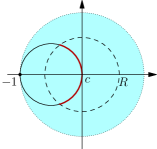
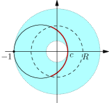
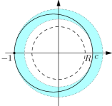
Figure 2. Shear parameter and analytic continuation. The solid circle is the image of the line $\mathrm{i}x_{2}+E$ under the Cayley type-transformation (4.16). The shadowed region with dotted boundary (the annulus with radii $c$ and $1$) is obtained from the solid circle under rotation around the origin. The dashed circle of the radius $R$ bounds the domain of the analytic continuation of the solution (4.15).
The left picture corresponds to $E=m\omega$ (thus $c=0$)—there always exists a part of the shaded region inside the circle of a radius $R$ (even for $R=0$).
The middle picture represents a case of some $E$ within the bound (4.18)—there is an arc (drawn by a thick pen) inside of the dashed circle. The arc corresponds to values of $x_{2}$ such that the solution (4.13) is meaningful.
The right picture illustrates the shear parameter $E$, which is outside of the range (4.18). For such a state, which is squeezed too much, no values of $x_{2}$ allow to use the region of the analytic continuation within the dashed circle.

The existence of bounds (4.18) for possible squeezing parameter $E$ shall be expected from the physical consideration. The integral formula (4.15) produces for a real $\mathrm{i}u$ a solution of the irreversible heat-diffusion equation for the time-like parameter $u$. However, its analytic extension into the complex plane will include also solutions of time-reversible Schrödinger equation for purely imaginary $\mathrm{i}u$. Since the rotation of the second variable in (4.13) requires all complex values of $u$ with fixed $\left|u\right|$, only a sufficiently small neighbourhood (depending on the “niceness” of an initial value $f_{2}(z,0)$) is allowed. Also note, that a rotation of a squeezed state in the phase space breaks the minimal uncertainty condition at certain times, however the state periodically “re-focus” back to the initial minimal uncertainty shape [Wodkiewicz87].

If a solution $f_{2}(z,u)$, $u\in\mathbb{R}{}$ of (4.15) does not permit an analytic expansion into a neighbourhood of the origin, then two analytic extensions $f^{\pm}_{2}(z,u)$, for $\Im u>0$ and $\Im u<0$ respectively, shall exist. Then, the dynamics in (4.13) will experience two distinct jumps for all values of $t$ such that

(4.19) $$\Re\left(\mathrm{e}^{-2\mathrm{i}\omega t}\frac{m\omega-(\mathrm{i}x_{2}+E)}{m\omega+(\mathrm{i}x_{2}+E)}\right)=0\,.$$

An analysis of this case and its physical interpretation is beyond the scope of the present paper.

5. Ladder operators on the group $\mathbb{G}{}$

For determining a complete set of eigenvectors of Hamiltonian  (4.7) we consider ladder operators. Let

$$a^{+}=\sqrt{\frac{m\omega}{\pi\hslash_{4}}}\left(\frac{\mathrm{i}}{2m\omega}X_{1}-\frac{1}{2}X_{3}\right)\quad\text{and}\quad a^{-}=\sqrt{\frac{m\omega}{\pi\hslash_{4}}}\left(\frac{\mathrm{i}}{2m\omega}X_{1}+\frac{1}{2}X_{3}\right).$$

Using the derived representation formulae (2.7) we have the following dimensionless operators:

$$L^{+}:=\mathrm{d}{\tilde{\rho}^{a^{+}}_{h_{4}}} =\sqrt{\frac{m\omega}{\pi\hslash_{4}}}\left(\frac{\mathrm{i}}{2m\omega}\mathrm{d}{\tilde{\rho}^{X_{1}}_{\hslash_{4}}}-\frac{1}{2}\mathrm{d}{\tilde{\rho}^{X_{3}}_{\hslash_{4}}}\right)$$

$$=\frac{\mathrm{i}}{2\sqrt{\pi m\omega\hslash_{4}}}(-\partial_{1}-(x_{2}+\mathrm{i}m\omega)\partial_{3}+2\pi\mathrm{i}\hslash_{4}x_{3}\,I);$$

$$L^{-}:=\mathrm{d}{\tilde{\rho}^{a^{-}}_{\hslash_{4}}} =\sqrt{\frac{m\omega}{\pi\hslash_{4}}}\left(\frac{\mathrm{i}}{2m\omega}\mathrm{d}{\tilde{\rho}^{X_{1}}_{\hslash_{4}}}+\frac{1}{2}\mathrm{d}{\tilde{\rho}^{X_{3}}_{\hslash_{4}}}\right)$$

$$=\frac{\mathrm{i}}{2\sqrt{\pi m\omega\hslash_{4}}}(-\partial_{1}-(x_{2}-\mathrm{i}m\omega)\partial_{3}+2\pi\mathrm{i}\hslash_{4}x_{3}\,I)\,.$$

One can immediately verify the commutator

(5.1) $$[L^{-},L^{+}]=I\,.$$

The Hamiltonian (4.7) is expressed in terms of the ladder operators:

(5.2) $$H=\hslash_{4}\omega(L^{+}L^{-}+\frac{1}{2}\,I)\,.$$

Thus the following commutators hold:

$$[H,L^{+}]=\hslash_{4}\omega L^{+},\quad[H,L^{-}]=-\hslash_{4}\omega L^{-}.$$

Moreover, creation and annihilation operators are adjoint of each other:

(5.3) $$(L^{-})^{*}=L^{+}$$

where ‘*’ indicates the adjoint of an operator in terms of the inner product defined by (3.9). Then, from (5.2) and (5.3) we see that $H^{*}=H$.

Now, for the function (see (3.24) for $q=m\omega$)

(5.4) $$\Phi_{0}(x_{1},x_{2},x_{3})=\frac{\sqrt{2}(m\omega E)^{1/4}}{\sqrt{\mathrm{i}x_{2}+E+m\omega}}\exp\left(-\pi{\hslash_{4}}Ex_{1}^{2}-2\pi\mathrm{i}h_{2}x_{2}-\pi{\hslash_{4}}\frac{(x_{3}-\mathrm{i}Ex_{1})^{2}}{\mathrm{i}x_{2}+E+m\omega}\right),$$

it can be easily checked that it is a vacuum vector in $\mathsf{L}_{\phi}{}(\mathbb{G}{}/Z)$:

$$L^{-}\Phi_{0}=0.$$

It is normalised ($\left\|\Phi_{0}\right\|_{x_{2}}=1$) and for the higher order normalised states, we put

$$\Phi_{j}=\frac{1}{\sqrt{j!}}(L^{+})^{j}\Phi_{0},\quad\quad j=1,2,\ldots.$$

Orthogonality of $\Phi_{j}$ follows from the fact that $H$ is self-adjoint. Then, for

$$z=\frac{x_{3}-\mathrm{i}Ex_{1}}{\mathrm{i}x_{2}+E+m\omega},\quad u=\frac{m\omega-(\mathrm{i}x_{2}+E)}{m\omega+(\mathrm{i}x_{2}+E)}$$

we have

(5.5) $$\Phi_{j}(z,u)=\frac{1}{\sqrt{2^{j}j!}}(-u)^{j/2}H_{j}\left(\sqrt{\frac{-2\pi\hslash_{4}m\omega}{u}}\;z\right)\Phi_{0}$$

where

(5.6) $$H_{j}(y)=\sum_{k=0}^{\lfloor\frac{j}{2}\rfloor}\frac{(-1)^{k}j!}{k!(j-2k)!}(2y)^{j-2k}$$

are the Hermite polynomials  [Folland89]*§ 1.7 [Andrews98a]*§ 5.2 and $\lfloor\cdot\rfloor$ is the floor function (i.e. for any real $x$, $\lfloor x\rfloor$ is the greatest integer $n$ such that $n\leq x$.) And,

$$\Phi_{0}(z,u) =\left(\frac{E}{m\omega}\right)^{1/4}\mathrm{e}^{2\pi h_{2}E}\sqrt{1-u}\exp\left(\frac{\pi\hslash_{4}Em^{2}\omega^{2}}{(1-u)^{2}}\big{(}z+(\frac{E}{m\omega}(-1+u)+u)\overline{z}\big{)}^{2}\right)$$

(5.7) $$\qquad\times\exp\left(\frac{-2\pi m\omega}{1-u}\big{(}h_{2}{(1+u)}+\hslash_{4}{z^{2}}\big{)}\right).$$

It is easy to show (by induction in which we use (5.1)) that

(5.8) $$L^{-}\Phi_{j}=[L^{-},\frac{1}{\sqrt{j!}}(L^{+})^{j}]\Phi_{0}=\sqrt{j}\Phi_{j-1}.$$

Therefore,

$$L^{+}L^{-}\Phi_{j}=j\Phi_{j}.$$

Hence, for the Hamiltonian $H$ of the harmonic oscillator  (4.7) we have

$$\textstyle H\Phi_{j}=\hslash_{4}\omega(j+\frac{1}{2})\ \Phi_{j}.$$

Furthermore, it can be verified that both operators $\mathcal{C}$ (3.18) and $\mathcal{S}$ (3.22) commute with the creation operator $L^{+}$ and thus

$$\mathcal{C}\Phi_{j}=\mathcal{S}\Phi_{j}=0,\quad j=0,1,2,\ldots.$$

Note, that singularity of eigenfunction (5.5) at $u=0$ is removable due to a cancellation between the first power factor and the Hermite polynomial given by (5.6). Moreover, the eigenfunction (5.5) has an analytic extension in $u$ to the whole complex plane, thus does not have any restriction on the squeezing parameter $E$ from the inequality (4.17).

The eigenfunction $\Phi_{j}(z,u)$ (5.5) at $u=0$ reduces to the power $z^{j}$ of the variable $z$, as can be expected from the connection to the FSB space and the Heisenberg group. The appearance of the Hermite polynomials in $\Phi_{j}(z,u)$ (5.5) may be a bit confusing since the Hermite functions represent eigenvectors in the Schrödinger representation over $\mathsf{L}_{2}{}(\mathbb{R}{})$. However, if we substitute the dynamic (4.13):

$$z_{t}=\frac{x_{3}-\mathrm{i}Ex_{1}}{\mathrm{i}x_{2}+E+m\omega}\mathrm{e}^{-\mathrm{i}\omega t},\qquad u_{t}=\frac{m\omega-(\mathrm{i}x_{2}+E)}{m\omega+(\mathrm{i}x_{2}+E)}\mathrm{e}^{-2\mathrm{i}\omega t}$$

into the eigenfunction (5.5) we get

$$\Phi_{j}(z_{t},u_{t})=\frac{1}{\sqrt{2^{j}j!}}(-u_{t})^{j/2}\,H_{j}\bigg{(}\sqrt{\frac{-2\pi\hslash_{4}m\omega}{u}}\;z\bigg{)}\Phi_{0}(z_{t},u_{t})\,.$$

Thus, the argument of Hermite function “stays still” while the time parameter is present only in the power factor and the vacuum (5). This is completely inline with the FSB space situation.

6. Discussion and conclusions

We presented a method to obtain a geometric solution of Schrödinger equation expressed through coordinate transformation. The method relays on coherent state transform based on group representations [Perelomov86] [AliAntGaz14a]*Ch. 7. It is shown that properties of the solution depends on a group and its representation used in the transform. The comparison of the Heisenberg and shear $\mathbb{G}{}$ groups cases shows that a larger group $\mathbb{G}{}$ creates the image space with a bigger number of auxiliary conditions. These conditions can be used to reduce the order of a partial differential equation with bigger flexibility, leading to a richer set of geometric solutions. We have seen that the fiducial vector for the Heisenberg group is uniquely defined while for the larger group $\mathbb{G}{}$ different minimal uncertainty states still lead to a geometric solution. There are some natural bounds (4.18) of a possible squeeze parameter, they are determined by the degree of singularity of the solution of the equation (4.14). It would be interesting to find a physical interpretation of jumps for values (4.19) for states which do not have an analytic continuation into a neighbourhood of the origin.

The present work provides a further example of numerous cases [Kisil09d, Kisil10c, Kisil98a, Zimmermann06, Guerrero18] when the coherent state transform is meaningful and useful beyond the traditional setup of square-integrable representations modulo a subgroup $H$ [AliAntGaz14a]*Ch. 8. Specifically, coherent states parametrised by points of the homogeneous space $\mathbb{G}{}/H$ are not sufficient to accommodate the dynamics (4.13).

It would be interesting to continue the present research for other groups. One of the immediate candidates was suggested to us by an anonymous referee: the Newton–Hook group [BacryLevy-Leblond68a, Streater67], which is the Heisenberg group added with time translations generated by the harmonic oscillator Hamiltonian. A more refined coherent state transform can be achieved by the Schrödinger group $\mathbb{S}{}$ introduced in § 2.3 because it is possibly the largest natural group for describing coherent states for the harmonic oscillator, see [AldayaCossioGuerreroLopez-Ruiz11b] [AldayaGuerrero01a] [Folland89]*Ch. 5. However, as was mentioned at the end of § 2.3, the smaller group $\mathbb{G}{}$ has more representations than the larger Schrödinger group. Thus advantages of each group for geometric description of dynamics needs to be carefully investigated.