Sensitivity Analysis of Cascaded Quantum Feedback Amplifier

Abstract

Quantum amplifier is an essential device in quantum information processing. As in the classical (non-quantum) case, its characteristic uncertainty needs to be suppressed by feedback, and in fact such a control theory for a single quantum amplifier has recently been developed. This letter extends this result to the case of cascaded quantum amplifier. In particular, we consider two types of structures: the case where controlled amplifiers are connected in series, and the case where a single feedback control is applied to the cascaded amplifier. Then, we prove that the latter is better in the sense of sensitivity to the uncertainty. A detailed numerical simulation is given to show actual performance of these two feedback schemes.

I Introduction

Amplifiers are essential in modern technology [1]. Note that this device is not used in a stand-alone fashion, because its amplification gain cannot be exactly specified due to unavoidable characteristic uncertainty. Actually the amplified output signal produced from a bare amplifier can be largely distorted, and eventually the performance of signal processing is degraded. Black discovered that feedback control resolves this issue [2], which has been further investigated in depth [3, 4]. This feedback amplification method, which is now known as one of the most successful examples of control theory, has made a significant contribution to the development of the today’s electronic technologies.

The idea of classical (non-quantum) feedback amplification is as follows. Figure 2 shows a system composed of a single amplifier with gain $G$ and another system (called the controller) with gain $K$. A simple calculation yields

$$y=G^{\rm fb}u,~{}~{}G^{\rm fb}=\frac{G}{1+GK}.$$ (1)

Therefore, in the limit $|G|\to\infty$, the closed-loop gain becomes $G^{\rm fb}\to 1/K$. This means that the robust amplification is realized by taking a passive and attenuating controller, such as a resistor, because the characteristic change in $K$ of those passive devices is in general quite small.

A single amplifier does not always provide sufficient gain and bandwidth due to the gain-bandwidth constraint, and thus cascaded amplifiers are often used in practice to satisfy the required performance [1]. Surely feedback stabilization is needed in this case as well, but it is not obvious how to construct a feedback configuration for such a multi-component network. In the classical control theory, as the most basic study, two types of feedback configurations depicted in Fig. 2 were first investigated. The type-a scheme shown in Fig. 2(a) is the cascade connection of the feedback-controlled amplifiers, and in the type-b scheme shown in (b), a single feedback loop is constructed for the cascaded amplifier. In [5], it was shown that the type-b scheme is more effective for improving the robustness than the type-a.

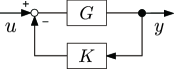
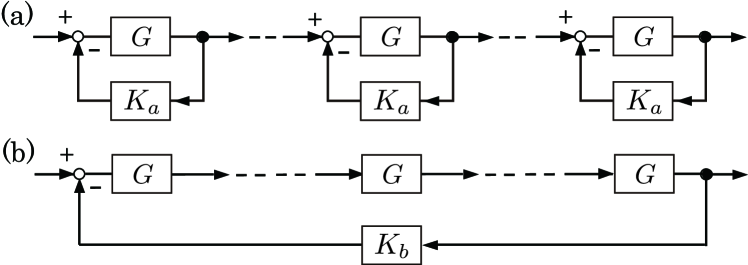
Figure 1: Feedback control for a classical amplifier.

Figure 2: Two basic feedback configurations for cascaded classical amplifier; type-a and type-b.

Turning our attention to the quantum regime, the quantum amplifier [6]–[9] is expected to serve as a fundamental device in quantum information science, such as quantum sensing [10]–[12] and quantum communication [13]–[15]. In practice, the quantum amplifier must be stabilized via feedback as in the classical case. In fact one of the authors has developed the theory of feedback stabilization for a single quantum amplifier [16]. It is thus important to extend the theory to the case of cascaded quantum amplifier [17]–[19], which has not been yet established; in particular, analyzing proper quantum versions of the above-described two classical feedback configurations should be an important basic study along this research direction. The contribution of this letter is to prove that a quantum version of the classical type-b scheme is better than a correspondence to the type-a, in the sense of the robustness. Note that, although this is the same conclusion as the classical one, the proof is non-trivial, because the quantum amplifier is essentially a multi-input and multi-output (MIMO) device and eventually the analysis becomes much more involved than the classical case, as will be shown in the letter.

This letter is organized as follows. Section II is devoted to some preliminaries. In Section III, we prove the main result. Section IV gives a detailed numerical simulation to show the robustness and stability of the controlled amplifiers.

II Preliminaries

II-A Sensitivity Function and Cascaded Classical Amplifier

Here we aim to quantify the robustness of the controlled amplifier described in Section I. Suppose that a small characteristic change $\Delta G$ occurs in the gain as $G\to G+\Delta G$. Then the closed-loop gain (1) changes to $G^{\rm fb}+\Delta G^{\rm fb}$. The sensitivity function of $G^{\rm fb}$ with respect to $G$ is defined as

$$S=\frac{\,\,\Delta G^{\rm fb}/G^{\rm fb}}{\Delta G/G}.$$ (2)

Now the small deviation $\Delta G^{\rm fb}$ is calculated as

$$\Delta G^{\rm fb}=\frac{G+\Delta G}{1+(G+\Delta G)K}-\frac{G}{1+GK}\approx\frac{\Delta G}{(1+GK)^{2}},$$

thus $S=1/(1+GK)$. Therefore, the open-loop gain $GK$ should be carefully designed so that $|S|<1$ while retaining the stability of the closed-loop system.

Next we consider the cascaded feedback amplifiers shown in Fig. 2 [5], which in both cases are composed of $N$ identical classical amplifiers. In the type-a scheme, the same feedback controller with gain $K_{a}$ is applied to each amplifier, and in the type-b scheme, the output of the terminal amplifier is fed back to the first one through the single controller with gain $K_{b}$. The overall gains are given by

$$G_{a}^{\rm fb}=(G^{\rm fb})^{N}=\frac{G^{N}}{(1+GK_{a})^{N}},~{}~{}G_{b}^{\rm fb}=\frac{G^{N}}{1+G^{N}K_{b}}.$$

Now suppose that the small change $G\to G+\Delta G$ occurs in one of the amplifiers, say, the $j$-th amplifier. Then the fluctuations of $G_{a}^{\rm fb}$ and $G_{b}^{\rm fb}$ are calculated as follows;

$$\Delta G_{a}^{\rm fb} =\frac{(G+\Delta G)G^{N-1}}{[1+(G+\Delta G)K_{a}](1+GK_{a})^{N-1}}-\frac{G^{N}}{(1+GK_{a})^{N}}$$

$$\approx\frac{G^{N-1}\Delta G}{(1+GK_{a})^{N+1}},$$

$$\Delta G_{b}^{\rm fb} =\frac{(G+\Delta G)G^{N-1}}{1+(G+\Delta G)G^{N-1}K_{b}}-\frac{G^{N}}{1+G^{N}K_{b}}\approx\frac{G^{N-1}\Delta G}{(1+G^{N}K_{b})^{2}}.$$

From Eq. (2), the sensitivity functions are given by

$$S_{a}=1/(1+GK_{a}),~{}~{}S_{b}=1/(1+G^{N}K_{b}).$$ (3)

Then, if the gains of both of the controlled systems are equal and these are smaller than the gain of the non-controlled cascaded amplifier, i.e., $|G^{\rm fb}_{a}|=|G^{\rm fb}_{b}|<|G|^{N}$, we have

$$\frac{|S_{b}|}{|S_{a}|}=\frac{1}{|1+GK_{a}|^{N-1}}<1.$$

Thus the type-b feedback scheme has a better performance than the type-a scheme in the sense of sensitivity.

II-B Quantum Amplifier and Feedback Stabilization

In this letter we consider the phase-preserving linear quantum amplifier [6]–[9], which is simply called the “amplifier” in what follows. Let $b(t)$ be a field annihilation operator called the signal; $b(t)$ has the meaning of a complex amplitude of the field and satisfies the canonical commutation relation (CCR) $b(t)b^{\dagger}(t^{\prime})-b^{\dagger}(t^{\prime})b(t)=\delta(t-t^{\prime})$, where $b^{{\dagger}}(t)$ represents the Hermitian conjugate of $b(t)$. The amplifier transforms $b(t)$ to $\tilde{b}(t)=gb(t)+\sqrt{g^{2}-1}\,d^{{\dagger}}(t)$, where $d(t)$ is an additional field annihilation operator called the idler, which is necessary to preserve the CCR of $\tilde{b}(t)$. Also $g>1$ is the amplification gain.

In quantum optics the non-degenerate parametric amplifier (NDPA) [20] shown in Fig. 3(a) is often used. This is an optical cavity with two inputs $b_{1}$ (signal) and $b_{2}$ (idler). The corresponding internal cavity modes $a_{1}$ and $a_{2}$ couple with each other at the pumped nonlinear crystal. In the rotating-frame at the half of input laser frequency, the dynamical equations of the NDPA under ideal setup (i.e., zero-detuned and no-loss) are given by

$$\dot{a}_{1}=-\frac{\kappa}{2}a_{1}+\varepsilon a_{2}^{{\dagger}}-\sqrt{\kappa}b_{1},~{}\dot{a}_{2}^{{\dagger}}=-\frac{\kappa}{2}a_{2}^{{\dagger}}+\varepsilon a_{1}-\sqrt{\kappa}b_{2}^{{\dagger}},$$

$$\tilde{b}_{1}=\sqrt{\kappa}a_{1}+b_{1},~{}~{}\tilde{b}_{2}^{{\dagger}}=\sqrt{\kappa}a_{2}^{{\dagger}}+b_{2}^{{\dagger}},$$

where $\kappa$ is the cavity damping rate and $\varepsilon$ is the strength of nonlinearity. (The mirror ${\rm M}_{i}$ is partially transmissive for $a_{i}$ but perfectly reflective for the other cavity mode.)

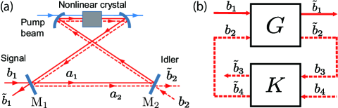
Figure 3: (a) Non-degenerate parametric amplifier. (b) Feedback configuration for a single quantum amplifier.

In the Laplace domain, the amplified output signal $\tilde{b}_{1}$ is, together with the amplified idler $\tilde{b}_{2}$, represented as

$$\left[\begin{array}[]{c}\tilde{b}_{1}(s)\\ \tilde{b}_{2}^{{\dagger}}(s)\\ \end{array}\right]=\left[\begin{array}[]{cc}g_{1}(s)&g_{2}(s)\\ g_{2}(s)&g_{1}(s)\\ \end{array}\right]\left[\begin{array}[]{c}b_{1}(s)\\ b_{2}^{{\dagger}}(s)\\ \end{array}\right],$$ (4)

where $g_{1}(s)=(s^{2}-\kappa^{2}/4-\varepsilon^{2})/D(s)$ and $g_{2}(s)=-\kappa\varepsilon/D(s)$ are the transfer functions with $D(s)=s^{2}+\kappa s+\kappa^{2}/4-\varepsilon^{2}$. Note that $|g_{1}(i\omega)|^{2}-|g_{2}(i\omega)|^{2}=1,~{}\forall\omega$ holds to satisfy the CCR of the output, represented by $\tilde{b}(i\omega)\tilde{b}^{\dagger}(i\omega^{\prime})-\tilde{b}^{\dagger}(i\omega^{\prime})\tilde{b}(i\omega)=\delta(\omega-\omega^{\prime})$ in the Fourier domain. Also the characteristic equation $D(s)=0$ yields the stability condition $0<x=2\varepsilon/\kappa<1$. The gain at the center frequency satisfies $|g_{1}(0)|=(1+x^{2})/|1-x^{2}|\to\infty$ as $x\to 1-0$.

Here we review the general feedback method for a single quantum amplifier [16]. The general linear quantum amplifier is represented in the Laplace domain as [21]:

$$\left[\begin{array}[]{c}\tilde{b}_{1}(s)\\ \tilde{b}_{2}^{{\dagger}}(s)\\ \end{array}\right]=G(s)\left[\begin{array}[]{c}b_{1}(s)\\ b_{2}^{{\dagger}}(s)\\ \end{array}\right],~{}G(s)=\left[\begin{array}[]{cc}G_{11}(s)&G_{12}(s)\\ G_{21}(s)&G_{22}(s)\\ \end{array}\right],$$

where $|G_{11}(i\omega)|^{2}-|G_{12}(i\omega)|^{2}=|G_{22}(i\omega)|^{2}-|G_{21}(i\omega)|^{2}=1$ and $G_{21}(i\omega)G_{11}^{*}(i\omega)-G_{22}(i\omega)G_{12}^{*}(i\omega)=0$ hold for all $\omega$. As for the controller, we take a passive and attenuating quantum system with the following input-output relation:

$$\left[\begin{array}[]{c}\tilde{b}_{3}^{{\dagger}}(s)\\ \tilde{b}_{4}^{{\dagger}}(s)\\ \end{array}\right]=K(s)\left[\begin{array}[]{c}b_{3}^{{\dagger}}(s)\\ b_{4}^{{\dagger}}(s)\\ \end{array}\right],~{}K(s)=\left[\begin{array}[]{cc}K_{11}(s)&K_{12}(s)\\ K_{21}(s)&K_{22}(s)\\ \end{array}\right].$$

$K^{{\dagger}}(i\omega)K(i\omega)=I,~{}\forall\omega$ holds to satisfy the CCR in both $\tilde{b}_{3}$ and $\tilde{b}_{4}$. These two systems are connected through the feedback $b_{2}=\tilde{b}_{4}$ and $b_{3}=\tilde{b}_{2}$, as shown in Fig. 3(b). The input-output relation of the closed-loop system is given by

$$\left[\begin{array}[]{c}\tilde{b}_{1}(s)\\ \tilde{b}_{3}^{{\dagger}}(s)\\ \end{array}\right]=\left[\begin{array}[]{cc}G^{\rm fb}_{11}(s)&G^{\rm fb}_{12}(s)\\ G^{\rm fb}_{21}(s)&G^{\rm fb}_{22}(s)\\ \end{array}\right]\left[\begin{array}[]{c}b_{1}(s)\\ b_{4}^{{\dagger}}(s)\\ \end{array}\right],$$ (5)

where

$$G^{\rm fb}_{11} =[G_{11}-K_{21}(G_{11}G_{22}-G_{12}G_{21})]/(1-G_{22}K_{21}),$$

$$G^{\rm fb}_{12} =G_{12}K_{22}/(1-G_{22}K_{21}),~{}~{}G^{\rm fb}_{21}=G_{21}K_{11}/(1-G_{22}K_{21}),$$

$$G^{\rm fb}_{22} =[K_{12}+G_{22}(K_{11}K_{22}-K_{12}K_{21})]/(1-G_{22}K_{21}).$$

Then $|G^{\rm fb}_{11}(s)|\to 1/|K_{21}(s)|>1$ holds in the high-gain limit $|G_{11}|\to\infty$, meaning that the amplification process can be made robust by feedback as in the classical case.

III Cascaded quantum feedback amplifier

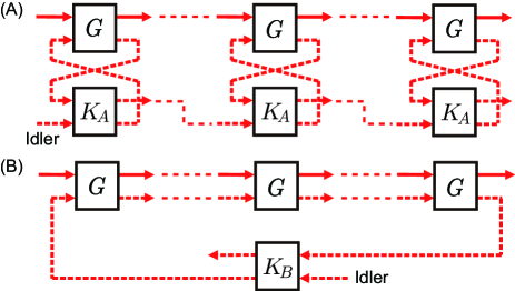
Figure 4: Two basic feedback configurations for cascaded quantum amplifier; type-A and type-B.

In this section we show the quantum version of the classical cascade amplification theory given in Section II-A. First note that, because the quantum amplifier is an MIMO system and hence it essentially differs from the classical one, specifying the feedback network composed of amplifiers and controllers, which corresponds to the classical one shown in Fig. 2, is a non-trivial problem. Here we particularly consider the case where the idler mode of the amplifier can be used, in addition to the signal mode, to construct the feedback network; actually in the standard experiments of quantum optics [20] and superconductivity [22], the idler mode is artificially implemented and is thus accessible. In this formulation, reasonable quantum versions of the classical feedback networks are illustrated in Fig. 4; the type-A and type-B schemes correspond to the classical type-a and type-b schemes, respectively. In both cases, the signal-out and the idler-out are connected to the signal-in and the idler-in, respectively, and eventually the whole system has only one idler input from outside. Note that, if the idler modes are not accessible and only the signal modes can be connected, then in both configurations the whole closed-loop system has multiple idler inputs and eventually it is subjected to a large noise coming from those idler input channels.

Now the problem is to compare the sensitivity of the two schemes shown in Fig. 4. We tackle this problem under the following setting. First, we focus on the gain at the center frequency $\omega=0$. Then we consider the quantum amplifier whose transfer function matrix at $\omega=0$ is of the form

$$G(0)=\left[\begin{array}[]{cc}G_{1}&G_{2}\\ G_{2}&G_{1}\\ \end{array}\right],~{}~{}G_{1}^{2}-G_{2}^{2}=1,~{}~{}G_{i}\in{\mathbb{R}}.$$ (8)

Note that the ideal NDPA with transfer functions (4) indeed fulfills this condition. Moreover we suppose that both feedback networks are composed of $N$ identical quantum amplifiers characterized by Eq. (8), and that the gain of only the $j$-th amplifier changes as $G_{1}\to G_{1}+\Delta G_{1}$ and $G_{2}\to G_{2}+\Delta G_{2}$. Lastly, without loss of generality, the transfer function matrix of the controller at $\omega=0$ can be set to:

$$K_{\bullet}(0)=\left[\begin{array}[]{cc}K_{1\bullet}&K_{2\bullet}\\ -K_{2\bullet}&K_{1\bullet}\\ \end{array}\right],~{}K_{1\bullet}^{2}+K_{2\bullet}^{2}=1,~{}~{}K_{i\bullet}\in{\mathbb{R}},$$

where $\bullet=A,B$; i.e., $K_{A}(0)$ and $K_{B}(0)$ are applied to the type-A and the type-B schemes, respectively.

First, we derive the overall gain for the type-A scheme. From Eq. (5), each feedback-controlled amplifier has the following transfer function matrix:

$$G^{\rm fb}(0) =\left[\begin{array}[]{cc}G^{\rm fb}_{1}&G^{\rm fb}_{2}\\ G^{\rm fb}_{2}&G^{\rm fb}_{1}\\ \end{array}\right]$$

$$=\frac{1}{1+G_{1}K_{2A}}\left[\begin{array}[]{cc}G_{1}+K_{2A}&G_{2}K_{1A}\\ G_{2}K_{1A}&G_{1}+K_{2A}\\ \end{array}\right].$$

This matrix can be diagonalized using the orthogonal matrix $P=1/\sqrt{2}[1,1;1,-1]$ as follows;

$$P^{-1}G^{\rm fb}(0)P={\rm diag}\{\lambda^{\rm fb}_{+},~{}\lambda^{\rm fb}_{-}\}=\left[\begin{array}[]{cc}\lambda^{\rm fb}_{+}&0\\[3.0pt] 0&\lambda^{\rm fb}_{-}\\ \end{array}\right],$$

where $\lambda^{\rm fb}_{\pm}=(G_{1}+K_{2A}\pm G_{2}K_{1A})/(1+G_{1}K_{2A})$. The overall transfer function matrix is the $N$ product of $G^{\rm fb}(0)$;

$$G_{A}^{\rm fb} \equiv\left[\begin{array}[]{cc}G^{\rm fb}_{1A}&G^{\rm fb}_{2A}\\[3.0pt] G^{\rm fb}_{2A}&G^{\rm fb}_{1A}\\ \end{array}\right]=[G^{\rm fb}(0)]^{N}$$

$$=\frac{1}{2}\left[\begin{array}[]{cc}(\lambda^{\rm fb}_{+})^{N}+(\lambda^{\rm fb}_{-})^{N}&(\lambda^{\rm fb}_{+})^{N}-(\lambda^{\rm fb}_{-})^{N}\\[3.0pt] (\lambda^{\rm fb}_{+})^{N}-(\lambda^{\rm fb}_{-})^{N}&(\lambda^{\rm fb}_{+})^{N}+(\lambda^{\rm fb}_{-})^{N}\\ \end{array}\right].$$

The gain of interest is the (1,1) element of $G_{A}^{\rm fb}$, i.e., $G^{\rm fb}_{{\scriptstyle 1A}}$. Now the characteristic changes $G_{1}\to G_{1}+\Delta G_{1}$ and $G_{2}\to G_{2}+\Delta G_{2}$ occur; then, using $G_{2}\Delta G_{2}=G_{1}\Delta G_{1}$, we find that the fluctuation of $G^{\rm fb}_{1A}$ is calculated as

$$\Delta G^{\rm fb}_{1A} =\frac{1}{2}\left[\frac{G_{1}+\Delta G_{1}+K_{2A}+(G_{2}+\Delta G_{2})K_{1A}}{1+(G_{1}+\Delta G_{1})K_{2A}}\right.$$

$$~{}~{}~{}~{}~{}~{}~{}~{}~{}~{}\left.-~{}\frac{G_{1}+K_{2A}+G_{2}K_{1A}}{1+G_{1}K_{2A}}\right]\left(\lambda^{\rm fb}_{+}\right)^{N-1}$$

$$~{}~{}~{}~{}+\frac{1}{2}\left[\frac{G_{1}+\Delta G_{1}+K_{2A}-(G_{2}+\Delta G_{2})K_{1A}}{1+(G_{1}+\Delta G_{1})K_{2A}}\right.$$

$$~{}~{}~{}~{}~{}~{}~{}~{}~{}~{}\left.-~{}\frac{G_{1}+K_{2A}-G_{2}K_{1A}}{1+G_{1}K_{2A}}\right]\left(\lambda^{\rm fb}_{-}\right)^{N-1}$$

$$\approx\frac{K_{1A}\Delta G_{1}}{2G_{2}(1+G_{1}K_{2A})}\left[\left(\lambda^{\rm fb}_{+}\right)^{N}-\left(\lambda^{\rm fb}_{-}\right)^{N}\right].$$

As a result, the sensitivity function is represented as

$$S_{A}=\frac{\,\,\Delta G^{\rm fb}_{1A}/G^{\rm fb}_{1A}}{\Delta G_{1}/G_{1}}=\frac{K_{1A}G_{1}}{G_{2}(1+G_{1}K_{2A})}\frac{G^{\rm fb}_{2A}}{G^{\rm fb}_{1A}}.$$ (9)

Next we consider the type-B scheme, where the single feedback control is applied to the series of quantum amplifiers with transfer function matrix (8). Noting that $G(0)$ is diagonalized in terms of the orthogonal matrix $P$ as $P^{-1}G(0)P={\rm diag}\{\lambda_{+},~{}\lambda_{-}\}$ with $\lambda_{\pm}=G_{1}\pm G_{2}$, we have

$$[G(0)]^{N}=\left[\begin{array}[]{cc}M_{1}&M_{2}\\ M_{2}&M_{1}\\ \end{array}\right]=\frac{1}{2}\left[\begin{array}[]{cc}\lambda_{+}^{N}+\lambda_{-}^{N}&\lambda_{+}^{N}-\lambda_{-}^{N}\\[3.0pt] \lambda_{+}^{N}-\lambda_{-}^{N}&\lambda_{+}^{N}+\lambda_{-}^{N}\\ \end{array}\right].$$

From Eq. (5), the transfer function matrix of the whole closed-loop system is then given by

$$G_{B}^{\rm fb} \equiv\left[\begin{array}[]{cc}G^{\rm fb}_{1B}&G^{\rm fb}_{2B}\\[3.0pt] G^{\rm fb}_{2B}&G^{\rm fb}_{1B}\\ \end{array}\right]$$

$$=\frac{1}{1+M_{1}K_{2B}}\left[\begin{array}[]{cc}M_{1}+K_{2B}&M_{2}K_{1B}\\[3.0pt] M_{2}K_{1B}&M_{1}+K_{2B}\\ \end{array}\right].$$

The characteristic change in $G_{1}$ and $G_{2}$ induces a small fluctuation in the overall gain, $G^{\rm fb}_{1B}$, as follows:

$$\Delta G^{\rm fb}_{1B} =\frac{M_{1}+\Delta M_{1}+K_{2B}}{1+(M_{1}+\Delta M_{1})K_{2B}}-\frac{M_{1}+K_{2B}}{1+M_{1}K_{2B}}$$

$$=\frac{K_{1B}^{2}\Delta M_{1}}{(1+M_{1}K_{2B})[1+(M_{1}+\Delta M_{1})K_{2B}]}$$

$$=\frac{K_{1B}^{2}M_{2}\Delta G_{1}}{(1+M_{1}K_{2B})[G_{2}+(M_{1}G_{2}+M_{2}\Delta G_{1})K_{2B}]}$$

$$\approx\frac{K_{1B}G^{\rm fb}_{2B}\Delta G_{1}}{G_{2}(1+M_{1}K_{2B})},$$

where the following equality is used:

$$G_{2}\Delta M_{1}=M_{2}\Delta G_{1}.$$ (10)

The proof of this equation is given in Appendix. Therefore we arrive at the following sensitivity function:

$$S_{B}=\frac{\,\,\Delta G^{\rm fb}_{1B}/G^{\rm fb}_{1B}}{\Delta G_{1}/G_{1}}=\frac{K_{1B}G_{1}}{G_{2}(1+M_{1}K_{2B})}\frac{G^{\rm fb}_{2B}}{G^{\rm fb}_{1B}}.$$ (11)

Now we show the main result of this letter; if the gains of both of the controlled systems are equal and these are smaller than the gain of the non-controlled cascaded amplifier, i.e., $|G^{\rm fb}_{1A}|=|G^{\rm fb}_{1B}|<|M_{1}|$, we prove that

$$|S_{B}|<|S_{A}|.$$ (12)

The proof is given in Appendix. Therefore, the type-B feedback scheme is better than the type-A scheme in terms of the sensitivity to the characteristic uncertainty $\Delta G_{1}$.

Remark 1: Here we remark on a difference between the quantum and classical sensitivity functions. Because we aim to construct a high-gain feedback controlled amplifier, let us assume $|G^{\rm fb}_{1\bullet}|\gg 1$ ($\bullet=A,B$). Then, due to $|G^{\rm fb}_{1\bullet}|^{2}-|G^{\rm fb}_{2\bullet}|^{2}=1$, Eqs. (9) and (11) are then approximated as

$$S_{A}\approx\frac{K_{1A}G_{1}}{G_{2}(1+G_{1}K_{2A})},~{}~{}~{}S_{B}\approx\frac{K_{1B}G_{1}}{G_{2}(1+M_{1}K_{2B})}.$$

Now further let us take $|G_{1}|\gg 1$; then, from $G_{1}^{2}-G_{2}^{2}=1$, the quantum sensitivity function $S_{\bullet}$ is identical to the classical one (3) except for $K_{1\bullet}$. However, the idea of cascade amplification is to connect many low-gain amplifiers in series to realize $|G^{\rm fb}_{1\bullet}|\gg 1$ (e.g., Case 4 in Section IV); in this case $G_{1}/G_{2}$ takes a large value, and eventually $S_{\bullet}$ can become bigger than the classical one or even 1. In the classical case, this type of performance degradation does not occur, which is due to the increase of $G_{1}/G_{2}$; note that this term stems from the CCR constraint on quantum mechanical systems.

IV Stability and sensitivity analysis

TABLE I: Nominal parameters and the resulting sensitivity.

	Case1	Case2	Case3	Case4
$N$	$2$		$5$
$M_{1}$ [dB]	45	30	45	30
$x$	0.90	0.78	0.53	0.393
$\beta_{\scriptscriptstyle A}$	0.2	0.1	0.07	0.03
$\beta_{\scriptscriptstyle B}$	$-0.0412$	$-0.0291$	0.0034	0.0046
$S_{A}$	0.3388	0.7259	1.0718	1.4094
$S_{B}$	0.1190	0.5271	0.7428	1.2802
$g_{m}$ [dB]	8.1310	18.4593	8.5699	19.9847

The superiority of the type-B scheme over the type-A is guaranteed to hold only at the center frequency $\omega=0$. Thus, in this section, we focus on a specific system and numerically investigate the frequency dependence of amplification gain in those two schemes, with particular attention to the robustness and stability properties.

The amplifier is the ideal NDPA discussed in Section II-B. The controller is a partially transmissive mirror called the beam-splitter (BS), which is a 2-inputs and 2-outputs passive static system with the following transfer function matrix:

$$K_{\bullet}(s)=\left[\begin{array}[]{cc}\alpha_{\bullet}&-\beta_{\bullet}\\ \beta_{\bullet}&\alpha_{\bullet}\\ \end{array}\right],~{}~{}\alpha_{\bullet}^{2}+\beta_{\bullet}^{2}=1,$$

where $\bullet=A,B$. The real parameters $\alpha_{\bullet},\beta_{\bullet}\in{\mathbb{R}}$ represent the transmissivity and reflectivity of the mirror, respectively. Note that, from Eq. (5), the single NDPA with this controller has the amplification gain $1/|\beta_{\bullet}|$ in the limit $x\to 1-0$.

We consider the four cases summarized in Table I; the number of amplifiers is $N=2$ (Cases 1 and 2) or $N=5$ (Cases 3 and 4); the gain of the (1,1) element of $[G(0)]^{N}$, i.e., the non-controlled cascaded NDPA at $\omega=0$, is $M_{1}=45$ dB (Cases 1 and 3) or $M_{1}=30$ dB (Cases 2 and 4). In each case the cavity decay rate of the NDPA is fixed to $\kappa=1.8\times 10^{7}$ Hz [23, 24], while $x=2\varepsilon/\kappa$ is chosen so that $M_{1}$ equals to 45 dB or 30 dB. The reflectivity $\beta_{B}$ was determined as follows; first we fix the parameters of the type-A system, $x$ and $\beta_{A}$, and then $\beta_{B}$ is determined so that the gains at $\omega=0$ of both of the schemes are the same, i.e., $|G^{\rm fb}_{1A}|=|G^{\rm fb}_{1B}|$.

First, let us see the stability of the feedback-controlled system. For the type-A system, it is enough to analyze the stability of the single feedback-controlled NDPA; its characteristic equation is given by

$$s^{2}+\frac{\kappa}{1-\beta_{A}}s+\frac{1+\beta_{A}}{1-\beta_{A}}\frac{\,\,\kappa^{2}}{4}-\varepsilon^{2}=0.$$

The system is stable if and only if both of the two solutions $s$ of this equation satisfy ${\rm Re}(s)<0$, which leads to $x=2\varepsilon/\kappa<\sqrt{(1+\beta_{A})/(1-\beta_{A})}$. This condition is always satisfied if the NDPA is stable ($x<1$) and $0\leq\beta_{A}<1$.

To analyze the stability property of the type-B system, we use the Nyquist plot, which is now directly applicable because all the parameters ($\kappa,\varepsilon,\alpha_{B},\beta_{B}$) are real. The Nyquist plot is the vector plot of the open-loop transfer function $L(s)$, i.e., the trajectory of $({\rm Re}\{L(i\omega)\},{\rm Im}\{L(i\omega)\})$ with $\omega\in(-\infty,+\infty)$; note that $L(s)=G(s)K(s)$ for the classical system (1). The feedback-controlled system is stable if and only if there is no encirclement of the point $(-1,0)$, provided that $L(s)$ has no unstable poles. Now, from Eq. (5) the type-B system has the open-loop transfer function $L(s)=-[G^{N}]_{22}(s)\beta_{B}$, where $[G^{N}]_{22}(s)$ is the (2,2) element of $G(s)^{N}$. The Nyquist plots are shown in Fig. 5; hence, from the above stability criterion, the type-B system is stable in all Cases.

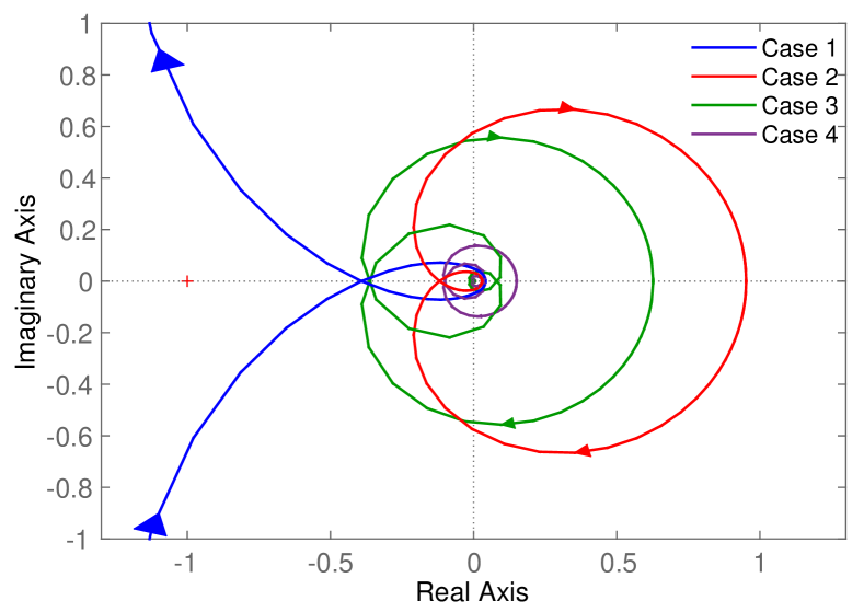
Figure 5: Nyquist plots of the type-B controlled system.

Next we discuss the sensitivity. To see this explicitly, suppose that the characteristic change of the amplifier, $\Delta G_{1}$, stems from the fluctuation of the parameter $\varepsilon$. We model this uncertainty as $\varepsilon^{\prime}=(1+0.05r)\varepsilon$, where $r$ is the random number generated from the uniform distribution over $[-1,1]$; that is, the nominal parameter $x=2\varepsilon/\kappa$ given in Table I experiences up to 5$\%$ deviation. The gain plots are shown in Fig. 6, where the red and blue lines represent the gains of the type-A and the type-B systems, respectively. Also the black lines are the gain plots of the cascaded amplifier without feedback. In each scheme (color), 100 sample paths are produced from the above-mentioned probability distribution. The figure shows that, in all Cases, the gain fluctuation of the controlled systems at $\omega=0$ are smaller than that of the uncontrolled system; that is, the feedback control always works well to suppress the gain fluctuation of the amplifier, at the price of decreasing the gain. Moreover, the fluctuation of the gain at $\omega=0$ of the type-B controlled system is always smaller than that of the type-A, i.e., $|S_{B}|<|S_{A}|$, as proven in Section III. However, importantly, this fact does not hold over all frequencies; in particular in Cases 1 and 3, the type-A scheme is better than the type-B, at the frequency $\omega\sim\kappa/10$ where there is a peaking in the gain.

(a) $N=2,\,M_{1}\approx 45\,{\rm[dB]}$ (b) $N=2,\,M_{1}\approx 30\,{\rm[dB]}$

(c) $N=5,\,M_{1}\approx 45\,{\rm[dB]}$ (d) $N=5,\,M_{1}\approx 30\,{\rm[dB]}$

Figure 6: Gain plots of the feedback-controlled system.

Finally we discuss the control performance, with the focus on both stability and sensitivity. The Nyquist plot can be used to quantify how much the system is stable, in terms of the gain margin $g_{m}=1/|L(i\omega_{pc})|$ with $\omega_{pc}$ the phase crossover frequency satisfying $\angle L(i\omega_{pc})=-180^{\circ}$. Now, as shown in Table I, the gain margin $g_{m}$ in Cases 1 and 3 are smaller than that in Cases 2 and 4. Hence the systems in Cases 1 and 3 are less stable than those in Cases 2 and 4; actually a peaking appears in Figs. 6(a) and (c), but not in (b) and (d). However, as implied by Fig. 6, it is harder to reduce the sensitivity in Cases 2 and 4, compared to Cases 1 and 3. That is, there is a tradeoff between the stability and robustness. Note also that the controlled system with less number of amplifiers has the better sensitivity; in fact the controlled system composed of $N=5$ amplifiers, which yet has the same level of sensitivity as that of the system with $N=2$, is often unstable.

V Concluding remark

The long-term goal of this work is to develop the design theory for feedback-controlled quantum networks containing amplifiers, corresponding to the established classical one [1]–[5]. Toward this goal, as an important first step, this letter gives the following theorem: to construct a robust high-gain quantum amplifier from some low-gain amplifiers, it is always better to stabilize the cascaded amplifier via a single feedback controller, than to take a cascade connection of feedback-controlled amplifiers. Recall that, although this is the same conclusion as the classical one, the proof of this fact is highly non-trivial. Also, as stated in Remark 1 and shown in Section IV, the sensitivity functions of the quantum feedback amplifiers have different characteristic from the classical counterparts in robustness and stability. As a consequence, a more careful sensitivity analysis will be required in general for designing a practical quantum network device, e.g., a robust quantum communication channel over a specific bandwidth [13]–[15].

First we prove Eq. (10). If the gain of the $j$-th amplifier changes as $G_{1}\to G_{1}+\Delta G_{1}$ and $G_{2}\to G_{2}+\Delta G_{2}$, then $M_{1}=(\lambda_{+}^{N}+\lambda_{-}^{N})/2$ changes as follows;

$$\Delta M_{1} =\frac{1}{2}\,\Bigl{[}(G_{1}+\Delta G_{1}+G_{2}+\Delta G_{2})\lambda_{+}^{N-1}\Bigr{.}$$

$$~{}~{}~{}~{}~{}~{}~{}~{}~{}\Bigl{.}+(G_{1}+\Delta G_{1}-G_{2}-\Delta G_{2})\lambda_{-}^{N-1}\Bigr{]}-M_{1}$$

$$=\frac{1}{2}\,\Bigl{[}(\Delta G_{1}+\Delta G_{2})\lambda_{+}^{N-1}+(\Delta G_{1}-\Delta G_{2})\lambda_{-}^{N-1}\Bigr{]}$$

$$=\frac{\Delta G_{1}}{2}\Biggl{[}\left(1+\frac{G_{1}}{G_{2}}\right)\lambda_{+}^{N-1}+\left(1-\frac{G_{1}}{G_{2}}\right)\lambda_{-}^{N-1}\Biggr{]}$$

$$=\frac{\Delta G_{1}}{2G_{2}}\Bigl{[}\lambda_{+}^{N}-\lambda_{-}^{N}\Bigr{]}=\frac{M_{2}}{G_{2}}\,\Delta G_{1}.$$

Next we prove Eq. (12). To make a fair comparison, we assume that both the controlled systems have the same amplification gain at $\omega=0$, i.e., $|G^{\rm fb}_{1A}|=|G^{\rm fb}_{1B}|$, which leads to $|G^{\rm fb}_{2A}|=|G^{\rm fb}_{2B}|$. Then we have

$$\frac{|S_{B}|}{|S_{A}|}=\left|\frac{K_{1B}}{K_{1A}}\frac{1+G_{1}K_{2A}}{1+M_{1}K_{2B}}\right|=\left|\frac{1+G_{1}K_{2A}}{K_{1A}}\right|\left|\frac{\left(\lambda^{\rm fb}_{+}\right)^{N}-\left(\lambda^{\rm fb}_{-}\right)^{N}}{\lambda_{+}^{N}-\lambda_{-}^{N}}\right|.$$

Here, from the relations $a^{n}-b^{n}=(a-b)\sum_{k=1}^{n}a^{n-k}b^{k-1}$ and $\lambda_{+}\lambda_{-}=\lambda^{\rm fb}_{+}\lambda^{\rm fb}_{-}=1$, we have

$$\left(\lambda^{\rm fb}_{+}\right)^{N}-\left(\lambda^{\rm fb}_{-}\right)^{N}$$

$$= \left(\lambda^{\rm fb}_{+}-\lambda^{\rm fb}_{-}\right)\Bigl{[}\left(\lambda^{\rm fb}_{+}\right)^{N-1}+\left(\lambda^{\rm fb}_{+}\right)^{N-3}+\cdots+\left(\lambda^{\rm fb}_{+}\right)^{-(N-1)}\Bigr{]}$$

$$= \frac{2G_{2}K_{1A}}{1+G_{1}K_{2A}}{\sum^{N}_{k=1}\left(\lambda^{\rm fb}_{+}\right)^{N-2k+1}},$$

and likewise $\lambda_{+}^{N}-\lambda_{-}^{N}=2G_{2}{\sum^{N}_{k=1}\lambda_{+}^{N-2k+1}}$. Hence, $|S_{B}|/|S_{A}|$ is now expressed as

$$\frac{|S_{B}|}{|S_{A}|}=\left|\frac{\sum^{N}_{k=1}\left(\lambda^{\rm fb}_{+}\right)^{N-2k+1}}{\sum^{N}_{k=1}\lambda_{+}^{N-2k+1}}\right|.$$ (13)

In addition to the condition $|G^{\rm fb}_{1A}|=|G^{\rm fb}_{1B}|$, we assume that the gains of both of the type-A and type-B controlled systems are smaller than the gain of the non-controlled cascaded amplifier; $|G^{\rm fb}_{1A}|=|G^{\rm fb}_{1B}|<|M_{1}|$, which is represented as

$$\frac{|G^{\rm fb}_{1A}|}{|M_{1}|}=\left|\frac{\left(\lambda^{\rm fb}_{+}\right)^{k}+\left(\lambda^{\rm fb}_{+}\right)^{-k}}{\lambda_{+}^{k}+\lambda_{+}^{-k}}\right|<1,~{}~{}\forall k=1,\cdots,N.$$

Then, if $N$ is odd, Eq. (13) leads to

$$\frac{|S_{B}|}{|S_{A}|} =\left|\frac{1+\sum^{(N-1)/2}_{k=1}\left[\left(\lambda^{\rm fb}_{+}\right)^{2k}+\left(\lambda^{\rm fb}_{+}\right)^{-2k}\right]}{1+\sum^{(N-1)/2}_{k=1}\left(\lambda_{+}^{2k}+\lambda_{+}^{-2k}\right)}\right|$$

$$=\frac{1+\sum^{(N-1)/2}_{k=1}\left[\left(\lambda^{\rm fb}_{+}\right)^{2k}+\left(\lambda^{\rm fb}_{+}\right)^{-2k}\right]}{1+\sum^{(N-1)/2}_{k=1}\left(\lambda_{+}^{2k}+\lambda_{+}^{-2k}\right)}<1.$$

Also, if $N$ is even, particularly $N=4l-2~{}(l=1,2,\cdots)$,

$$\frac{|S_{B}|}{|S_{A}|} =\left|\frac{\lambda^{\rm fb}_{+}+\left(\lambda^{\rm fb}_{+}\right)^{-1}}{\lambda_{+}+\lambda_{+}^{-1}}\right|\frac{1+\sum^{l-1}_{k=1}\left[\left(\lambda^{\rm fb}_{+}\right)^{4k}+\left(\lambda^{\rm fb}_{+}\right)^{-4k}\right]}{1+\sum^{l-1}_{k=1}\left(\lambda_{+}^{4k}+\lambda_{+}^{-4k}\right)},$$

and if $N=4l~{}(l=1,2,\cdots)$,

$$\frac{|S_{B}|}{|S_{A}|} =\left|\frac{\lambda^{\rm fb}_{+}+\left(\lambda^{\rm fb}_{+}\right)^{-1}}{\lambda_{+}+\lambda_{+}^{-1}}\right|\frac{\sum^{l}_{k=1}\left[\left(\lambda^{\rm fb}_{+}\right)^{4k-2}+\left(\lambda^{\rm fb}_{+}\right)^{-(4k-2)}\right]}{\sum^{l}_{k=1}\left[\lambda_{+}^{4k-2}+\lambda_{+}^{-(4k-2)}\right]},$$

which are both less than $1$. This completes the proof.

References

• [1] J. G. Graeme, G. E. Tobey, and L. P. Huelsman, Operational Amplifiers: Design and Applications. New York, NY, USA: McGraw-Hill, 1971.
• [2] H. S. Black, “Stabilized feedback amplifiers,” Bell Syst. Tech. J., vol. 13, no. 1, pp. 1–18, Jan. 1934.
• [3] R. B. Blackman, “Effect of feedback on impedance,” Bell Syst. Tech. J., vol. 22, no. 3, pp. 269–277, Oct. 1943.
• [4] H. W. Bode, Network Analysis and Feedback Amplifier Design. Princeton, NJ, USA: D. Van Nostrand, 1945.
• [5] D. H. Horrocks, Feedback Circuits and Op. Amps, 2nd ed. London, U.K.: Chapman and Hall, 1990.
• [6] W. H. Louisell, A. Yariv, and A. E. Siegman, “Quantum fluctuations and noise in parametric processes. I,” Phys. Rev., vol. 124, no. 6, pp. 1646–1654, 1961.
• [7] B. R. Mollow and R. J. Glauber, “Quantum theory of parametric amplification. I,” Phys. Rev., vol. 160, no. 5, pp. 1076–1096, 1967.
• [8] A. A. Clerk, M. H. Devoret, S. M. Girvin, F. Marquardt, and R. J. Schoelkopf, “Introduction to quantum noise, measurement, and amplification,” Rev. Mod. Phys., vol. 82, no. 2, pp. 1155–1208, 2010.
• [9] C. M. Caves, J. Combes, Z. Jiang, and S. Pandey, “Quantum limits on phase-preserving linear amplifiers,” Phys. Rev. A, vol. 86, no. 6, 2012, Art. no. 063802.
• [10] C. M. Caves, “Quantum mechanics of measurements distributed in time. II. Connections among formulations,” Phys. Rev. D, vol. 35, no. 6, pp. 1815–1830, 1987.
• [11] B. Abdo, F. Schackert, M. Hatridge, C. Rigetti, and M. Devoret, “Josephson amplifier for qubit readout,” Appl. Phys. Lett., vol. 99, no. 16, 2011, Art. no. 162506.
• [12] B. Abdo, et al., “Josephson directional amplifier for quantum measurement of superconducting circuits,” Phys. Rev. Lett., vol. 112, no. 16, 2014, Art. no. 167701.
• [13] S. Pirandola, R. Laurenza, C. Ottaviani, and L. Banchi, “Fundamental limits of repeaterless quantum communications,” Nat. Commun., vol. 8, Apr. 2017, Art. no. 15043.
• [14] H. Qi and M. M. Wilde, “Capacities of quantum amplifier channels,” Phys. Rev. A, vol. 95, no. 1, 2017, Art. no. 012339.
• [15] H. Elemy, “A one-way quantum amplifier for long-distance quantum communication,” Quantum Inf. Process., vol. 16, no. 5, 2017, Art. no. 134.
• [16] N. Yamamoto, “Quantum feedback amplification,” Phys. Rev. Applied, vol. 5, no. 4, 2016, Art. no. 044012.
• [17] Z. Yan, X. Jia, X. Su, Z. Duan, C. Xie, and K. Peng, “Cascaded entanglement enhancement,” Phys. Rev. A, vol. 85, no. 4, 2012, Art. no. 040305.
• [18] W. P. He and F. L. Li, “Generation of broadband entangled light through cascading nondegenerate optical parametric amplifiers,” Phys. Rev. A, vol. 76, no. 1, 2007, Art. no. 012328.
• [19] D. Wang, Y. Zhang, and M. Xiao, “Quantum limits for cascaded optical parametric amplifiers,” Phys. Rev. A, vol. 87, no. 2, 2013, Art. no. 023834.
• [20] Z. Y. Ou, S. F. Pereira, and H. J. Kimble, “Realization of the Einstein-Podolsky-Rosen paradox for continuous variables in nondegenerate parametric amplification,” Appl. Phys. B, vol. 55, no. 3, pp. 265–278, 1992.
• [21] J. E. Gough, M. R. James, and H. I. Nurdin, “Squeezing components in linear quantum feedback networks,” Phys. Rev. A, vol. 81, no. 2, 2010, Art. no. 023804.
• [22] B. Yurke, et al., “Observation of 4.2-K equilibrium-noise squeezing via a Josephson-parametric amplifier,” Phys. Rev. Lett., vol. 60, no. 9, pp. 764–767, 1988.
• [23] S. Iida, M. Yukawa, H. Yonezawa, N. Yamamoto, and A. Furusawa, “Experimental demonstration of coherent feedback control on optical field squeezing,” IEEE Trans. Autom. Control, vol. 57, no. 8, pp. 2045–2050, Aug. 2012.
• [24] O. Crisafulli, N. Tezak, D. B. S. Soh, M. A. Armen, and H. Mabuchi, “Squeezed light in an optical parametric oscillator network with coherent feedback quantum control,” Opt. Exp., vol. 21, no. 15, pp. 18371–18386, 2013.