Monitoring near-Earth-object discoveries for imminent impactors

Abstract

Aims. We present an automated system called neoranger that regularly computes asteroid-Earth impact probabilities for objects on the Minor Planet Center’s (MPC) Near-Earth-Object Confirmation Page (NEOCP) and sends out alerts of imminent impactors to registered users. In addition to potential Earth-impacting objects, neoranger also monitors for other types of interesting objects such as Earth’s natural temporarily-captured satellites.

Methods. The system monitors the NEOCP for objects with new data and solves, for each object, the orbital inverse problem, which results in a sample of orbits that describes the, typically highly-nonlinear, orbital-element probability density function (PDF). The PDF is propagated forward in time for seven days and the impact probability is computed as the weighted fraction of the sample orbits that impact the Earth.

Results. The system correctly predicts the then-imminent impacts of 2008 TC₃ and 2014 AA based on the first data sets available. Using the same code and configuration we find that the impact probabilities for objects typically on the NEOCP, based on eight weeks of continuous operations, are always less than one in ten million, whereas simulated and real Earth-impacting asteroids always have an impact probability greater than 10% based on the first two tracklets available.

1 Introduction

We have set up an automated system called neoranger that is built on OpenOrb (Granvik et al. 2009) and computes asteroid-Earth impact probabilities for new or updated objects on the Near-Earth-Object Confirmation Page (NEOCP) provided by the Minor Planet Center (MPC). The orbit-computation methods used by neoranger are optimized for cases where the amount of astrometry is scarce or it spans a relatively short time span.

The main societal benefit of monitoring for imminent impactors is that it allows for a warning to be sent out in case of an immiment impact that can no longer be prevented. Two well-known examples of damage-causing impacts are the Tunguska (Chyba et al. 1993) and Chelyabinsk (Popova et al. 2013) airbursts. Neither of these two asteroids hit the surface of the Earth intact but instead disrupted in the atmosphere with the resulting shock waves being responsible for the damage on the ground. While the Tunguska event in 1908 destroyed a wide forested area, it did not cause any injuries because it happened in a sparsely populated area. The Chelyabinsk event in 2013, on the other hand, took place in an urban area injuring many residents and causing damage to buildings. The Chelyabinsk asteroid was undetected before its entry into the atmosphere, because it arrived from the general direction of the Sun.

The primary scientific benefit of discovering asteroids prior to their impact with the Earth is that it allows for the characterization of the impactor in space prior to the impact event. Cross-correlating spectroscopic information and the detailed mineralogical information obtained from the meteorites found at the impact location allows us to extend the detailed mineralogical information to all asteroids by using the spectroscopic classification of asteroids as a proxy. Only two asteroids have been discovered prior to entry into the Earth’s atmosphere, 2008 TC₃ (Jenniskens et al. 2009) and 2014 AA (Farnocchia et al. 2016a). Both asteroids were small (no more than five meters across) and hence discovered only about 20 hours before impact. Whereas hundreds of observations were obtained of 2008 TC₃, only seven observations were obtained of 2014 AA. The impact location and time were accurately predicted in advance for 2008 TC₃ whereas for 2014 AA the accurate impact trajectory was reconstructed afterwards using both astrometric observations and infrasound data. Meteorite fragments were recovered across the impact location for 2008 TC₃ whereas no meteorite fragments could be collected for 2014 AA, which fell into the Atlantic Ocean. Spectroscopic observations in visible wavelengths were obtained for 2008 TC₃ suggesting that the object is a rare F-type. Mineralogical analysis of one of the fifteen recovered meteorites showed it to be an anomalous polymict ureilite and thereby established a link between F-type asteroids and ureilites (Jenniskens et al. 2009).

Let us make the simplifying assumption that meteorites will be produced in the impacts of all asteroids larger than one meter in diameter. Brown et al. (2002, 2013) estimate that five-meter-diameter or larger asteroids (that is, similar to 2008 TC₃) impact the Earth once every year. Since about 70% of the impacts happen above oceans and roughly 50% of the impactors will come from the general direction of the Sun, our crude estimate is that an event similar to the impact of 2008 TC₃ (pre-impact spectroscopic observations and discovery of meteorites) will happen approximately twice in a decade. Since not all of the incoming asteroids are detected, our estimate is to be considered optimistic. This is also supported by the fact that there has not been another 2008 TC₃ -like event in the past decade. These rates imply that it will take at least a millennium to get a statistically meaningful sample of, say, ten events for each of the approximately 20 Bus-DeMeo spectral classes. However, the rate of events can be increased if the surveys could detect smaller objects prior to their impact.

The Asteroid Terrestrial-impact Last Alert System (ATLAS, Tonry et al. 2018) seeks to provide a warning time in the order of tens of hours for a Chelyabinsk-size object. ATLAS currently consists of two telescopes in the Hawaiian Islands with plans to build additional observatories in other parts of the world. The cameras of these two telescopes have extremely wide fields of view compared to other contemporary Near-Earth-Object (NEO) survey systems, and they scan the sky in less depth but more quickly producing up to 25,000 asteroid detections per night. The European Space Agency’s (ESA) fly-eye telescope is a similar concept with very large field of view. First light is expected in 2018 and it will be the first telescope in a proposed future European network that would scan the sky for NEOs. We stress that both ATLAS and ESA’s fly-eye telescopes have been funded primarily to reduce the societal risks associated to small asteroids impacting the Earth.

Pushing the detection threshold down to one-meter-diameter asteroids will increase the discovery rate for Earth impactors by a factor of 40. A factor of five in physical size corresponds to three magnitudes and such an improvement will, optimistically, be provided by the Large Synoptic Survey Telescope (LSST) with first light in 2023. Since events similar to 2008 TC₃ will still be rare and the timescales short, it is of the utmost importance to identify virtually all impactors and do that as early as possible, that is, immediately after their discovery, to allow for spectroscopic follow-up. Another challenge will be to obtain useful spectroscopic data of small, fast-moving impactors; obtaining visible spectroscopy of 2008 TC₃ was a borderline case with a four-meter-class telescope.

An alternative approach to determine the compositional structure of the asteroid belt is to focus on meteorite falls and use their predicted trajectories prior to the impact to identify the most likely source region in the asteroid belt. Granvik & Brown (in preparation) use the observed trajectories of 25 meteorite-producing fireballs published to date to associate meteorite types to their most likely escape routes from the asteroid belt and the cometary region. We note that while this approach is indirect, because it lacks the spectroscopic observations prior to the impact, it results in substantially higher statistics per unit time.

Long-term (timescales ranging from months to centuries) asteroid impact monitoring is carried out by Jet Propulsion Laboratory’s (JPL’s) Sentry system (Chamberlin et al. 2001) and the University of Pisa’s close-approach monitoring system CLOMON2 (Chesley & Milani 1999). These automated systems are based on a similar algorithm (Milani et al. 2002, 2005; Farnocchia et al. 2015b) and run in parallel. The results are continuously compared to identify problematic cases that have to be scrutinized in greater detail by human operators.

Whereas the long-term impact monitoring is well-established, dedicated short-term (from hours to weeks) impact monitoring has only recently started receiving serious attention. Farnocchia et al. (2015a) implemented an automated system (Farnocchia et al. 2016b) to regularly analyze the objects on the MPC’s NEOCP with systematic ranging. Spoto et al. (2018) have developed a short-arc orbit computation method that also analyzes the objects on the NEOCP with systematic ranging. Also neoranger relies on the observations on the NEOCP, but the implementation and the orbit-computation method are different. As in the case for long-term impact monitoring, comparing the results of two or more systems doing the same analysis but using different techniques provides assurance that the results are valid. The very time-critical science described above underscores the need for accurate and complete monitoring. In addition to scientific utility, small impactors such as 2008 TC₃ and 2014 AA are valuable in comparing the predicted and actual impact location and time. These small, non-hazardous impactors thus allow the community to verify that the impact-monitoring systems work correctly.

neoranger also monitors for other types of interesting objects such as asteroids temporarily captured by the Earth-Moon system. Granvik et al. (2012) predict that there is a one-meter-diameter or larger NEO temporarily orbiting the Earth at any given time. The population of temporarily-captured natural Earth satellites (NES) are challenging to discover with current surveys because they are small in size and move fast when at a sufficiently small distance (Bolin et al. 2014). Asteroid 2006 RH₁₂₀ (Kwiatkowski et al. 2009) is to date the only NES confirmed not to be a man-made object. It is a few meters in diameter and therefore less challenging to discover compared to smaller objects.

In what follows we will first describe the real data available through NEOCP as well as the simulated data used for testing neoranger. Then we describe the neoranger system and the overall characteristics of the numerical methods used (with detailed descriptions to be found in the appendix). Finally, we present a selection of results and discuss their implications, and end with some conclusions and future avenues for improvement.

2 Data

The MPC is a clearinghouse for asteroid and comet astrometry obtained by observers worldwide. Based on an automatically computed probability of a discovered moving object being potentially a new NEO, it is placed on MPC’s NEOCP for confirmation through follow-up observations. Systems such as neoranger and JPL’s Scout system5 monitor the NEOCP for astrometry on new discoveries.

Once the orbital solution for a new object has been sufficiently well constrained to secure its orbital classification, the MPC issues a Minor Planet Electronic Circular (MPEC) where the discovery is published, and the object is removed from the NEOCP. Following the release of an MPEC long-term (typically up to 100 years into the future) impact-probability computations are undertaken by Sentry and CLOMON2.

2.1 Objects on the NEOCP

As the primary test data set, we use 2339 observation sets of 695 objects on the NEOCP between August 19 and October 12, 2015 (eight weeks). We use the term ”observation set” to refer to astrometric observations for a single object posted on the NEOCP within the last half an hour, that is, neoranger checks the NEOCP for updates every half an hour by default.

Of the 695 objects that appeared on the NEOCP, 260 objects eventually received an MPEC. The remaining 435 objects were not NEOs or other objects on peculiar orbits, did not receive enough follow-up observations to reveal their true nature, were linked to previously discovered asteroids, or were found to be artificial satellites or image artifacts. Zero percent (36%) of the 260 objects that received an MPEC (of the 435 objects that did not receive an MPEC) have only one observation set. Zero percent (36%) have two observation sets, that is, the object is updated once with more observations. Two percent (16%) have three observation sets and 51% (37%) four observation sets. A large part of the observations in our test data set were obtained by the Panoramic Survey Telescope and Rapid Response System (Pan-STARRS) 1 (F51) as well as the Catalina Sky Survey (703) and the Mt. Lemmon Survey (G96). The first observation set for an object contains observations from only one observatory. Seventy-seven percent of the 695 objects have at least two observation sets, in which case for 91% of the objects the first two observation sets come from different observatories. Fifty-five percent of the 695 objects have at least three observation sets, in which case for 91% of the objects the first three observation sets come from three observatories. An observation set typically contains three or four observations. The time span of an observation set for Pan-STARRS 1 is typically 30–60 min, and for the Catalina Sky Survey and the Mt. Lemmon Survey 15–30 min. The time between two observation sets ranges from about 30 min to two days. The total time span when including up to four observation sets is typically between two hours and three days.

2.2 Simulated Earth impactors

Apart from the two known Earth impactors mentioned in the introduction, there are no real impactors for testing neoranger. Therefore we tested neoranger with 50 simulated objects that were randomly picked from the simulated sample generated by Vereš et al. (2009). We generated synthetic astrometry by using the location and the typical, but simplified, cadence of Pan-STARRS 1. For 30 simulated impactors we generated three astrometric observations with a 0.01 day interval between the observations about five days prior to the impact with the Earth. Then we generated three more astrometric observations for the next night, that is, four days before the impact. For the remaining 20 simulated impactors we did the same but generated four astrometric observations instead of three.

2.3 Geocentric objects

Similarly to Earth impactors, we have very few known NESs. Therefore we test the system’s capability to identify NESs with one asteroid temporarily captured by the Earth, 2006 RH₁₂₀, and also the space observatory Spektr-R. 2006 RH₁₂₀ was a natural temporarily-captured orbiter, which orbited the Earth from July 2006 until July 2007. For 2006 RH₁₂₀ we used 17 observations between September 16 and 17 2006 spanning 24 hours divided into four tracklets. The heliocentric elements at the end of the epoch used are $a=1.04$ AU, $e=0.031$, and $i=1.43^{\circ}$ and the geocentric elements are $a=0.013$ AU, $e=0.56,$ and $i=64.2^{\circ}$. Spektr-R (or RadioAstron) is a Russian Earth-orbiting space observatory (Kardashev et al. 2013). For Spektr-R we used eight observations on April 4 2016 spanning four hours divided into three tracklets. The geocentric elements are $a=180,000$ km, $e=0.93$, and $i=38.8^{\circ}$ at the end of the epoch used.

3 Methods

3.1 Statistical ranging

In statistical orbital ranging (Virtanen et al. 2001; Muinonen et al. 2001), the typically non-Gaussian orbital-element probability density is examined using Monte Carlo selection of orbits in orbital-element space using the Bayesian formalism. In practice, the statistical ranging method proceeds in the following way. Two observations are selected from the data set and random deviates are added to the four plane-of-sky coordinates to mimic observational noise. Next, topocentric distances are generated for the two observation dates. The noisy sky-plane coordinates and the two topocentric distances are transformed, by accounting for the observatory’s heliocentric coordinates at the observation dates, into two heliocentric position vectors that are mapped into the phase space of a Cartesian state vector, which is equivalent to a set of orbital elements (e.g., Keplerian elements). The proposed orbit is then used to compute ephemerides for all observation dates. In Monte Carlo (MC) ranging the proposed orbit is accepted if it produces acceptable sky-plane residuals and the $\Delta\chi^{2}$ is small enough with respect to the until-then best-fit orbit. The two other ranging variants using Markov chains require a burn-in phase, which ends when, for random walk (Muinonen et al. 2016), the first orbit with acceptable $\Delta\chi^{2}$ is found, and for Markov-Chain Monte Carlo (MCMC, Oszkiewicz et al. 2009), the first orbit with acceptable residuals at all dates is found. We use a constant prior probability-density function (PDF) with Cartesian state vectors.

The different variants (MC, MCMC, and random-walk) of the statistical orbital ranging method (Appendix A) used here have been implemented in the open-source orbit-computation software package OpenOrb. The ranging method in general has been tested with several large-scale applications, demonstrating its wide applicability to various observational data (see Virtanen et al. 2015, and references therein).

The systematic ranging used by Scout (Farnocchia et al. 2015a) scans a grid in the space of topocentric range $\rho$ and range rate $\dot{\rho}$. For each grid point a fit in right ascension and declination as well as their time derivatives ($\alpha$, $\delta$, $\dot{\alpha}$, $\dot{\delta}$) is computed by minimizing a cost function created from the observed-computed residuals and, combined with the topocentric range and range rate, these six are equivalent to a complete set of orbital elements. Farnocchia et al. (2015a) also tested different priors to be used with their analysis and concluded that a uniform prior produces the best results. The choice of an adequate prior distribution is critical to ensuring that impacting asteroids are identified as early as possible. In what follows we will use the uniform prior because that has been our default for many years and now also Farnocchia et al. (2015a) have shown that it is indeed a good choice. An alternative implementation of the systematic ranging was recently proposed by Spoto et al. (2018).

3.2 neoranger system description

The neoranger system evaluates the Earth-impact probability and various other characteristics of objects on the NEOCP. The automated system works in general as follows. neoranger checks the NEOCP every 30 min for new objects and old objects with new data. We note that the frequency of checks is a tunable parameter and can be changed, but we have empirically found out that 30 min is a reasonable update frequency for our current monitoring purposes.

For each observation set the different ranging methods are run (with a timeout of twenty minutes) in the following order until the requested number of sample orbits are computed: Monte Carlo (MC), Markov-Chain Monte Carlo (MCMC), and random-walk ranging (Appendix A). Previous orbit solutions are provided as input to ranging to constrain the initial range bounds and speed up the computations. For each observation set that results in the requested number of accepted sample orbits, the orbital-element PDF is propagated forward in time for seven days to derive the impact parameter distribution. We note that also the length of the forward propagation is a configuration parameter that can be changed if deemed necessary. The computing time required increases roughly linearly with the length of the forward propagation. The time needed to identify impactors can be reduced by dividing the integrations according to a logarithmic sequence, say, one, three, ten, and 30 days, so that, for example, the alert for an asteroid impacting within a day can be sent out after the first integration rather than waiting for the 30 day integration to finish. The impact probability is computed as the weighted fraction of impact orbits. Similarly, the probability of the object being geocentric is computed by transforming the heliocentric orbital elements to geocentric orbital elements, and computing the ratio of those orbits that have geocentric $e<1$.

The neoranger system sends out a notification by e-mail of all cases where the impact probability or the probability for an object being captured in an orbit about the Earth is greater than $10^{-4}$. We will next explain how this critical value and the required number of sample orbits have been determined.

4 Results

4.1 Configuration parameters

We used conservative values for the many adjustable configuration parameters in OpenOrb to be less sensitive to outliers in the first data sets and to allow for the widest possible orbital-element distribution. For the astrometric uncertainty we therefore assumed one arcsecond for all observatories. The configuration parameter that has the largest influence on the computing time is the required number of sample orbits. Since the number of sample orbits also directly affects the reliability of the results, we decided to carry out tests to find a suitable number. After 50,000 orbits the probabilities start to converge when gradually increasing the number of required sample orbits towards 100,000 (Fig. 1). We therefore fixed the number of required sample orbits to 50,000, because this is a good compromise between computing time and the consistency of the results.

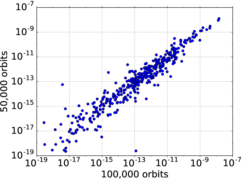
Figure 1: Impact probabilities for 398 objects with 100,000 and 50,000 orbits as the number of required sample orbits.

4.2 Earth impactors

We tested the system with the two known Earth impactors (2008 TC₃ and 2014 AA) and 50 objects from the simulated sample generated by Vereš et al. (2009). For the latter we generated synthetic astrometry for two consecutive nights as explained in Sect. 2.2. To compute the sample orbits the MC ranging was run twice: first with the observations of the first night, and then with the observations of both nights initializing the analysis with the orbits from the first ranging. The orbital-element probability density function resulting from the ranging is propagated forward in time as explained in Sect. 3.2. We found a strong correlation between the impact probability and the number of impacting orbits for the simulated impactors (Fig. 2). This implies that high impact probabilities are based on a statistically meaningful number of sample orbits, and are thus unlikely to be false alarms. We note that we do not here account for the fact that the typical false alarm is caused by a so-called outlier observation, an astrometric observation with the corresponding residual substantially larger than the expected astrometric uncertainty. The smallest impact probability is 10%, ten objects have a probability less than 50%, and 32 objects have a probability greater than 90%. For the nights with four astrometric observations the impact probabilities do not increase systematically compared to the nights with three observations.

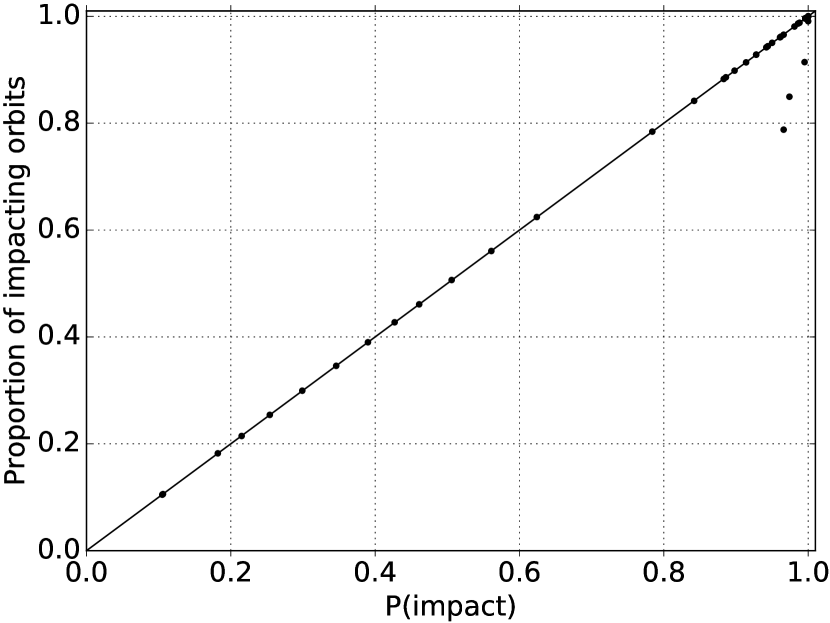
Figure 2: For 50 simulated impactors, the impact probability versus the fraction of impacting orbits. The solid black line is included for reference and corresponds to a 100% correlation between the fraction of impacting orbits and the impact probability.

When testing neoranger with the two known impactors, 2008 TC₃ and 2014 AA, we use two tracklets built from the first data sets available. For 2008 TC₃ we use the first observations obtained by R. Kowalski: for the first tracklet four observations and for the second tracklet three additional observations. For 2014 AA we use three observations for the first tracklet and the remaining four observations available for the second tracklet. For the first tracklet the ranging takes one minute and for the second tracklet ten minutes for both objects. With the addition of the second tracklet the propagation takes a considerably longer time, an hour for 2008 TC₃ and an hour and a half for 2014 AA), because due to many impacting orbits the integration steps become smaller. For both objects the impact probabilities are negligible (less than one in ten billion) when using only the first tracklet with a uniform prior, but increase to 81% and 60%, respectively, with Jeffreys’ prior. The apparent discrepancy with the results obtained with a uniform prior by Farnocchia et al. (2015a) will be studied in detail in a forthcoming paper. With the addition of the second tracklet the impact probabilities increase to 92% for 2008 TC₃ and to 80% for 2014 AA. The two-dimensional (2D) marginal probability densities for semi-major axis and eccentricity for 2008 TC₃ and 2014 AA are shown in Fig. 7. The PDFs resulting from the ranging method correctly cover the region where the ”true” orbit based on all available data (marked with a star) resides.

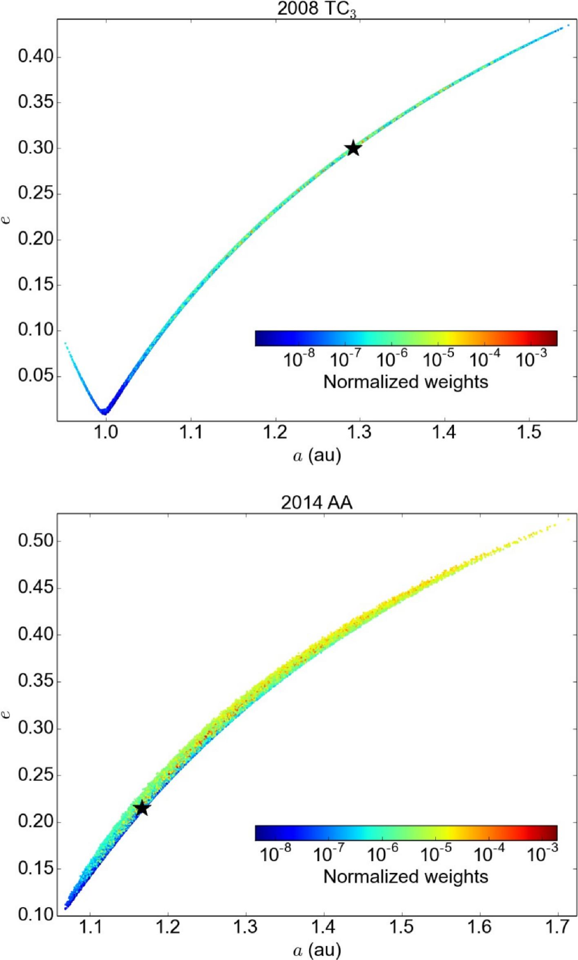
Figure 3: Two-dimensional marginal probability densities for semi-major axis and eccentricity for the impactors 2008 TC₃ (epoch 54745.8 MJD) and 2014 AA (epoch 56658.3 MJD) based on the first seven observations for both objects. The ”true” orbital elements for the chosen epoch based on all available data as reported by JPL’s HORIZONS system are marked with a star. We note that the estimate for 2014 AA also includes infrasound data (Farnocchia et al. 2016a).

In Fig. 4 the red histogram on the right represents 2008 TC₃, 2014 AA, and 50 simulated objects using two observation sets from consecutive nights. The green histogram represents 50 simulated objects using only one observation set. Hence it is clear that the substantially increased impact probability when adding a single data set to the discovery data set is typical for all impactors rather than being a random occurence for 2008 TC₃ and 2014 AA.

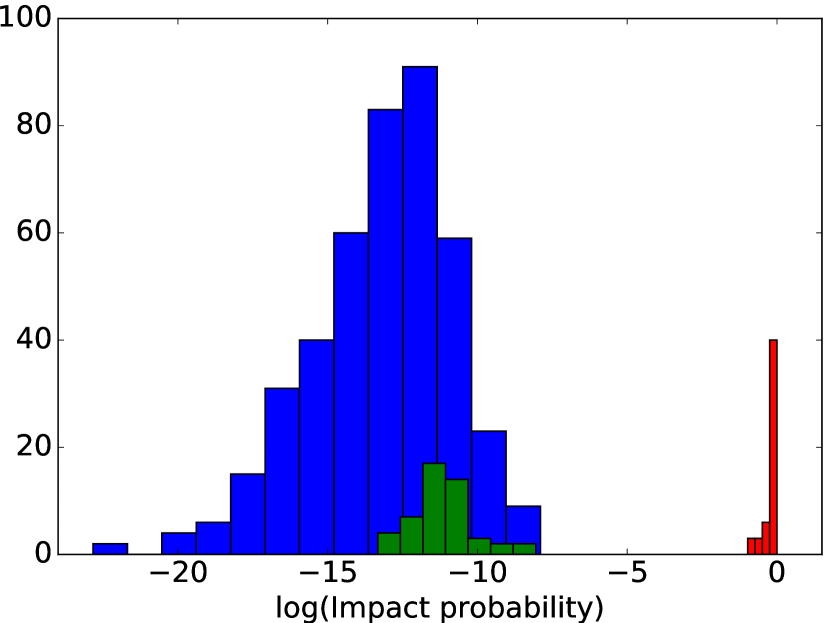
Figure 4: Impact probabilities for NEOCP objects during eight weeks of continuous monitoring (blue), for 50 simulated impactors using one observation set (green), and for 2008 TC₃, 2014 AA, and 50 simulated impactors using two observation sets from consecutive nights (red).

4.3 Geocentric objects

In addition to potential Earth-impacting objects our system also monitors for Earth’s natural temporarily-captured satellites, that is, objects on elliptic, geocentric orbits (hereafter just geocentric orbits). Here we present results of tests with 2006 RH₁₂₀, an asteroid temporarily captured by the Earth, and the space observatory Spektr-R.

For 2006 RH₁₂₀ the first tracklet (four observations during three minutes) produces only a negligible probability for the object being geocentric, the second tracklet (nine observations during seven hours) a 23% probability, the third tracklet (14 observations during seven hours) a 97% probability, and the fourth tracklet (17 observations during 24 hours) a 100% probability. For Spektr-R the first tracklet (four observations during one hour) gives a 24% probability, the second tracklet (six observations during three hours) a 97% probability, and the third tracklet (eight observations during four hours) a 100% probability. From these two examples we see that our system recognizes a geocentric object only if both the time span and number of observations are sufficient.

4.4 NEOCP objects

Having verified that neoranger can identify Earth-impacting asteroids as well as objects on elliptical, geocentric orbits, we now present results of eight weeks of continuous operations between August 18 and October 12 2015 for objects on the NEOCP. For each object neoranger calculates the probability that the object will impact the Earth within a week as well as the probability that the object is on an elliptic, geocentric orbit. In addition, we compute an estimate for the perihelion distance and NEO class. We compare these results with those given by MPC.

We use 2339 observation sets of 695 objects on the NEOCP. To derive the impact parameter distribution the ranging is run for each observation set and the resulting orbital element probability density function is propagated forward in time for seven days as explained in Sect. 3.2. The ranging for the first observation set takes on average one minute with root-mean-square (RMS) deviation of three minutes, for the second observation set three minutes (RMS five minutes), for the third observation set six minutes (RMS seven minutes), and for the fourth observation set seven minutes (RMS eight minutes). The ranging gradually slows down or fails for observation sets with larger time spans and number of observations. If the ranging fails it is mostly because the timeout of 20 minutes is exceeded or because no acceptable sample orbits are found (e.g., because the residuals are too large compared to the assumed astrometric uncertainty). The time required for the propagation stays typically around 1.5 minutes.

A non-zero impact probability is computed for 424 observation sets (and in accordance with Virtanen & Muinonen (2006) almost always for the first observation set of the object). The blue histogram in Fig. 4 shows the distribution of all non-zero impact probabilities computed by neoranger during the eight weeks of continuous monitoring. The ten highest probabilities in the blue histogram fall between $7.7\times 10^{-10}$ and $2.3\times 10^{-8}$. There is a clear gap between, on one hand, the group formed by the 50 simulated impactors and the two real impactors and, on the other hand, the group formed by the NEOCP objects and the simulated impactors with only one observation set. It thus seems that impactors are clearly identified already based on only two observation sets, and neoranger produces very few, if any, false alarms.

A non-zero probability for the object being on an elliptic, geocentric orbit is computed for 727 observation sets. Some fraction of these objects correspond to artificial Earth-orbiting satellites. In particular, neoranger has computed a non-zero probability for a geocentric orbit for all artificial objects that have appeared on NEOCP and that have been identified as such on the various discussion forums.

The evolution of the perihelion-distance estimate with the increasing number of observation sets for the 260 objects that received an MPEC is shown in Fig. 5. The error bars define the 1$\sigma$ confidence interval. The accuracy increases with each new observation set as expected. Figure 6 shows examples of the perihelion-distance distributions for two objects. We note the substantially non-Gaussian distribution in the top left plot compared to the Gaussian distribution in the bottom left plot.

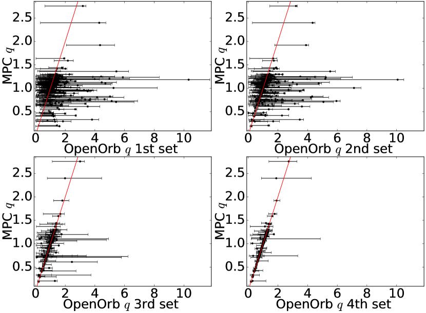
Figure 5: Perihelion distance as estimated by neoranger and by MPC. The MPC estimate is based on all available data whereas the neoranger estimate only includes parts of it as described below each plot. The solid red line is included for reference and corresponds to a 100% correlation between the perihelion distance as estimated by neoranger and by MPC.

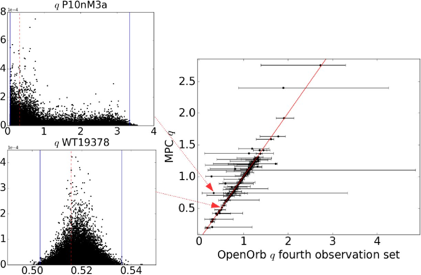
Figure 6: Two example distributions of the perihelion distance. The red vertical dashed line corresponds to the maximum likelihood and the blue vertical lines define the 1$\sigma$ confidence interval.

neoranger predicts the NEO class (Amor, Apollo, Aten, Aethra/Mars-crosser) correctly (i.e., neoranger estimates the class to be the one given by MPC with over 50% confidence) for 40% of the 260 objects in our test data set when using only the first observation set and 63% when using two observation sets (Fig. 7). In the rightmost bar in the plot for two tracklets we see that the correct class is predicted for $0.377*260=98$ objects with at least a 90% probability.

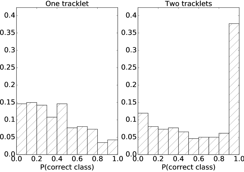
Figure 7: Fractional distribution of the probabilities (as estimated by neoranger) to belong to the class reported by the MPC when using one or two observation sets.

In rare cases (one object out of a thousand based on 13 months of operations) neoranger erroneously computes a high impact probability based on a small number of impacting orbits, as in the MCMC ranging run for 2017 JK₂ (Fig. 8). In that case, only 12 impacting orbits produce an impact probability of 2% although all the impacting orbits have large $\chi^{2}$ values. These impacting orbits also correspond to very small topocentric distances at the orbit computation epoch, which is typically the mid-point of the observational time span. These impacting orbits thus comprise the low-likelihood tail of the orbit distribution. In MCMC ranging the weight of a sample orbit is computed based on the repetitions, that is, the inability of the proposed orbit to be accepted when starting from the sample orbit in question. A viable scenario therefore is that, in some rare cases, the sample orbits in the tail get an unrealistically large number of repetitions, because there is essentially just one narrow path towards higher-likelihood orbits and the algorithm requires an unusually long time to find it. Since a large fraction of these close-in orbit solutions typically impact the Earth, the impact probability is also substantial despite the fact that the solutions have low likelihoods based on their $\chi^{2}$ values. The other two examples in Fig. 8 are the real impactor 2008 TC₃ and the simulated impactor Si000003 from Vereš et al. (2009). For 2008 TC₃ we get an impact probability of 98% with 48,293 impacting orbits (out of 50,000 orbits), and for Si000003 an impact probability of 24% with 11,691 impacting orbits.

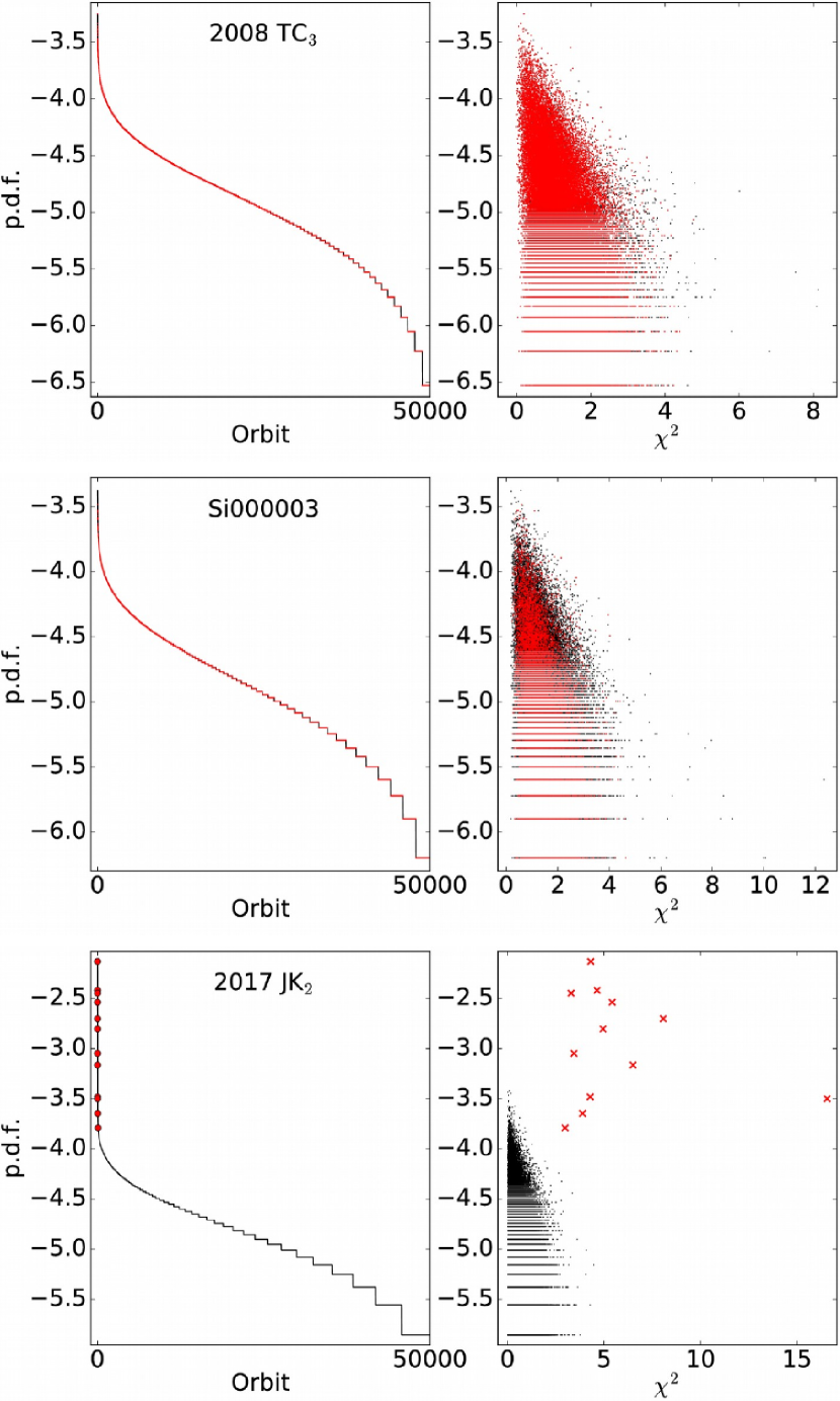
Figure 8: Distribution of PDFs and $\chi^{2}$ values for 2008 TC₃, Si000003, and 2017 JK₂ resulting from one MCMC ranging run. The red symbols represent the impacting orbits.

5 Conclusion

While neoranger correctly predicts the impacts of the two asteroids discovered before impacting the Earth, 2008 TC₃ and 2014 AA, the impact probabilities for objects on the NEOCP computed by neoranger are always less than one in ten million, as it should be for non-impactors typically found on NEOCP. In addition, neoranger rarely produces false alarms of impacting asteroids. As we gain experience from real objects we will be able to apply a threshold for an impact probability that should trigger follow-up efforts or, at least, close scrutiny of the data.

We note that, for the two known impactors (2008 TC₃ and 2014 AA) and 50 simulated impactors, a significant impact probability is achieved only using two tracklets while using only one tracklet results in a negligible impact probability. As a consequence our system might not be able to identify an impactor based on the very first data set available. It may be possible to increase the impact probability computed for the first observation set by using a uniform prior in polar coordinates (Farnocchia et al. 2015a). We leave the implementation and testing of the alternative prior(s) to future works that should also provide a quantitative comparison of the existing short-term impact-monitoring systems. Such a comparison would provide end-users with a fact-based list of pros and cons of the different systems.

Appendix A Statistical orbital ranging

A.1 Inverse problem of orbit computation

Within the Bayesian framework, the orbital-element probability density function (PDF) is

$$p_{\mathrm{p}}(\boldsymbol{P})\propto p_{\mathrm{pr}}(\boldsymbol{P})p_{\mathrm{\epsilon}}(\Delta\boldsymbol{\mathit{\Psi}}(\boldsymbol{P})),$$ (1)

where the prior PDF $p_{\mathrm{pr}}$ is constant and the observational error PDF $p_{\mathrm{\epsilon}}$ is evaluated for the observed–computed sky-plane residuals $\Delta\boldsymbol{\mathit{\Psi}}(\boldsymbol{P})$ and is typically assumed to be Gaussian (Muinonen & Bowell 1993). The parameters $\boldsymbol{P}$ describe the orbital elements of an asteroid at a given epoch $t_{0}$. For Keplerian orbital elements $\boldsymbol{P}=(a,e,i,\Omega,\omega,M_{0})^{T}$. For Cartesian elements, $\boldsymbol{P}=(X,Y,Z,\dot{X},\dot{Y},\dot{Z})^{T}$ , where, in a given reference frame, the vectors $(X,Y,Z)^{T}$ and $(\dot{X},\dot{Y},\dot{Z})^{T}$ denote the position and velocity, respectively.

A.2 Statistical ranging

In statistical orbital ranging (Virtanen et al. 2001; Muinonen et al. 2001), the orbital-element PDF is examined using Monte Carlo selection of orbits in orbital-element space in the following way:

• Select two observations (usually the first and the last) from the data set.

• To vary the topocentric coordinates R.A. and Dec., and the topocentric range of the two observations introduce six uniform random deviates mimicking uncertainties in the coordinates.

• Compute new Cartesian positions at the dates.

• For the proposed orbit, compute candidate orbital elements, R.A. and Dec. for all observation dates, and $\Delta\chi^{2}$.

• Let

  $$\Delta\chi^{2}(\boldsymbol{P})=\chi^{2}(\boldsymbol{P})-\chi^{2}(\boldsymbol{P}_{0})\,\mathrm{,and}$$ (2)

  $$\chi^{2}(\boldsymbol{P})=\Delta\boldsymbol{\mathit{\Psi}}^{T}(\boldsymbol{P})\Lambda^{-1}\Delta\boldsymbol{\mathit{\Psi}}(\boldsymbol{P})\,,$$

  where $\Lambda$ is the covariance matrix for the observational errors and $\boldsymbol{P}_{0}$ specifies a reference orbital solution. Notice that, for linear models and Gaussian PDFs, the definition of Eq. 2 yields the well-known result

  $$\Delta\chi^{2}(\boldsymbol{P})=(\boldsymbol{P}-\boldsymbol{P}_{0})^{T}\Sigma^{-1}(\boldsymbol{P}_{0})(\boldsymbol{P}-\boldsymbol{P}_{0}),$$ (3)

  where $\boldsymbol{P}_{0}$ denotes the linear least-squares orbital solution.

  In MC ranging proposed orbits are accepted if they produce acceptable sky-plane residuals: the $\Delta\chi^{2}$ value of the residuals is below a given threshold (we use 30), and if the residuals at all observation dates are smaller than given cutoff values (for $\Delta\alpha_{max}$ and $\Delta\delta_{max}$ we use 4 arcsecs). For the acceptance criteria of the other ranging variants see Sects. A.3 and A.4.

• If accepted, assign a statistical weight based on $\chi^{2}(\boldsymbol{P})$ describing the orbital-element PDF of the sample orbit:

  $$p_{\mathrm{p}}(\boldsymbol{P})\propto\mathrm{exp}\left[-\dfrac{1}{2}\chi^{2}(\boldsymbol{P})\right]\,.$$ (4)

• The procedure is repeated up to $10^{7}$ times resulting in up to 50,000 accepted sample orbits. Both of these are adjustable parameters and their current values have been found empirically (see Sect. 4.1).

A.3 MCMC ranging

Markov-chain Monte Carlo (MCMC) ranging (Oszkiewicz et al. 2009) is initiated with the selection of two observations from the full set of observations: typically, the first and the last observation are selected, denoted by A and B. Orbital-element sampling is then carried out with the help of the corresponding topocentric ranges ($\rho_{A}$, $\rho_{B}$), R.A.s ($\alpha_{A}$, $\alpha_{B}$), and Dec.s ($\delta_{A}$, $\delta_{B}$). These two spherical positions, by accounting for the light time, give the Cartesian positions of the object at two ephemeris dates. The two Cartesian positions correspond to a single, unambiguous orbit passing through the positions at the given dates.

For sampling the orbital-element PDF we utilize the Metropolis-Hastings (MH) algorithm. The MH algorithm is based on the computation of the ratio $a_{r}$:

$$a_{r}=\frac{p_{\mathrm{p}}(\boldsymbol{P^{\prime}})p_{\mathrm{t}}(\boldsymbol{P}_{j};\boldsymbol{P^{\prime}})}{p_{\mathrm{p}}(\boldsymbol{P}_{j})p_{\mathrm{t}}(\boldsymbol{P^{\prime}};\boldsymbol{P}_{j})}=\frac{p_{\mathrm{p}}(\boldsymbol{P^{\prime}})p_{\mathrm{t}}(\boldsymbol{Q}_{j};\boldsymbol{Q^{\prime}})J_{j}}{p_{\mathrm{p}}(\boldsymbol{P}_{j})p_{\mathrm{t}}(\boldsymbol{Q^{\prime}};\boldsymbol{Q}_{j})J^{\prime}}=\frac{p_{\mathrm{p}}(\boldsymbol{P^{\prime}})J_{j}}{p_{\mathrm{p}}(\boldsymbol{P}_{j})J^{\prime}},$$ (5)

where $\boldsymbol{P}_{j}$ and $\boldsymbol{Q}_{j}$ denote the current orbital elements and spherical positions, respectively, in a Markov chain, and the primed symbols, $\boldsymbol{P^{\prime}}$ and $\boldsymbol{Q^{\prime}}$, denote their proposals. The proposal PDFs from $\boldsymbol{P}_{j}$ to $\boldsymbol{P^{\prime}}$ and from $\boldsymbol{Q}_{j}$ to $\boldsymbol{Q^{\prime}}$ (t stands for transition) are, respectively, $p_{\mathrm{t}}(\boldsymbol{P^{\prime}};\boldsymbol{P}_{j})$ and $p_{\mathrm{t}}(\boldsymbol{Q^{\prime}};\boldsymbol{Q}_{j})$.

The proposal $\boldsymbol{P^{\prime}}$ is transformed to the space of two topocentric spherical positions $\boldsymbol{Q^{\prime}}=(\rho_{\mathrm{A}}^{\prime},\alpha_{\mathrm{A}}^{\prime},\delta_{\mathrm{A}}^{\prime},\rho_{\mathrm{B}}^{\prime},\alpha_{\mathrm{B}}^{\prime},\delta_{\mathrm{B}}^{\prime})^{\mathrm{T}}$ resulting in a multivariate Gaussian proposal PDF $p_{\mathrm{t}}(\boldsymbol{Q^{\prime}};\boldsymbol{Q}_{j})$. This transformation introduces Jacobians $J_{j}$ and $J^{\prime}$:

$$J_{j}=\left|\frac{\partial\boldsymbol{Q}_{j}}{\partial\boldsymbol{P}_{j}}\right|,\quad J^{\prime}=\left|\frac{\partial\boldsymbol{Q^{\prime}}}{\partial\boldsymbol{P^{\prime}}}\right|.$$ (6)

The ratio $a_{r}$ in Eq. 5 simplifies into its final form because the proposal PDFs $p_{\mathrm{t}}(\boldsymbol{Q_{j}};\boldsymbol{Q}^{\prime})$) and $p_{\mathrm{t}}(\boldsymbol{Q^{\prime}};\boldsymbol{Q}_{j})$) are symmetric.

The proposed elements $\boldsymbol{P^{\prime}}$ are accepted with the probability of min(1,$a_{r}$):

$$\mathrm{If\ }a_{r}\geq 1;\mathrm{\ then\ }\boldsymbol{P}_{j+1} =\boldsymbol{P^{\prime}}$$

$$\mathrm{If\ }a_{r}<1;\mathrm{\ then\ }\boldsymbol{P}_{j+1} =\boldsymbol{P^{\prime}}\mathrm{\ with\ probability\ }a_{r}$$

$$\boldsymbol{P}_{j+1} =\boldsymbol{P^{\prime}}\mathrm{\ with\ probability\ }1-a_{r}.$$ (7)

After a number of transitions in the so-called burn-in phase, the Markov chain, in the case of success, converges to sample the target PDF $p_{\mathrm{p}}$ when the first orbit with acceptable residuals at all dates is found.

The posterior distribution is proportional to the number of repetitions of a given orbit $r(\boldsymbol{P})$ rather than on the $\chi^{2}(\boldsymbol{P})$ values:

$$p_{\mathrm{p}}(\boldsymbol{P})\propto r(\boldsymbol{P})\,.$$ (8)

That is, the difficulty to find an acceptable $\boldsymbol{P^{\prime}}$ increases the probability of the current orbit $\boldsymbol{P}$.

A.4 Random walk ranging

Instead of MCMC ranging, it can be advantageous to sample in the entire phase-space regime below a given $\chi^{2}(\boldsymbol{P})$ level, assigning weights on the basis of the a posteriori probability density value and the Jacobians presented above (Muinonen et al. 2016, cf., Virtanen et al. 2001, Muinonen et al. 2001).

MCMC ranging can be modified for what we call random-walk ranging of the phase space within a given $\Delta\chi^{2}$ level. First, we assign a constant, nonzero PDF for the regime of acceptable orbital elements and assign a zero or infinitesimal PDF value outside the regime. MCMC sampling then returns a set of points that, after convergence to sampling the phase space of acceptable orbital elements (i.e., the burn-in phase ends when the first orbit with acceptable $\Delta\chi^{2}$ is found), uniformly characterizes the acceptable regime. Second, we assign the posterior PDF values $p_{\mathrm{p}}$ as the weights $w_{j}$ for the sample orbital elements $\boldsymbol{P}_{j}$. In the case of ranging using the topocentric spherical coordinates, the weights $w_{j}$ need to be further divided by the proper Jacobian value $J_{j}$.

In random-walk ranging, uniformly sampling the phase space of the acceptable orbital elements, the final weight factor for the sample elements $\boldsymbol{P_{j}}$ in the Markov chain is

$$w_{j}=\frac{r(\boldsymbol{P_{j}})}{J_{j}}\mathrm{exp}\left[-\dfrac{1}{2}\chi^{2}(\boldsymbol{P}_{j})\right].$$ (9)

We note that the same orbit can repeat itself in the chain, analogously to MCMC ranging.