Stochastic differential switching game in infinite horizon

Abstract

We study a zero-sum stochastic differential switching game in infinite horizon. We prove the existence of the value of the game and characterize it as the unique viscosity solution of the associated system of quasi-variational inequalities with bilateral obstacles. We also obtain a verification theorem which provides an optimal strategy of the game. Finally, some numerical examples with two regimes are given.

AMS subject classifications: 49N70, 49L25, 60H30, 90C39, 93E20

$\bf Keywords$: stochastic differential game, switching strategies, quasi-variational inequality, value function, viscosity solution

1 Introduction

Differential game theory involves multiple persons (also called players or individuals) decision making in the context of dynamic system. The study of the two-person zero-sum differential games could be traced back to the pioneering work by Isaacs [21], which inspired further research in this area.

In 1989, Fleming and Souganidis [15], for the first time, studied two-person zerosum stochastic differential games. They adopted the definitions of upper and lower value functions introduced by Elliott and Kalton [13] and proved that the two value functions satisfy the dynamic programming principle and they are the unique viscosity solutions to the associated Hamilton–-Jacobi–-Bellman–-Isaacs partial differential equations (HJBI PDEs). Their work generalized that of Evans and Souganidis [14] from the deterministic framework to the stochastic one and is now regarded as one of the outstanding results in the field of stochastic differential games. In 1995, Hamadène and Lepeltier [17] introduced the backward stochastic differential equation (BSDE) theory into the study of stochastic differential games, and there exist also many other works using this BSDEs approach, such as Hamadène, Lepeltier, and Peng [18]. Subsequently, Buckdahn and Li [2] extended the findings presented in [17, 18], and generalized the framework introduced in [15].

In this paper we consider the state process of the stochastic differential game, defined as the solution of the following stochastic equation:

$$\begin{array}[]{ll}X_{s}=x+\displaystyle\int_{t}^{s}b(r,X_{r},a_{t},b_{t})dr+\displaystyle\int_{t}^{s}\sigma(r,X_{r},a_{t},b_{t})dW_{r}\qquad s\geq t,\end{array}$$

with $X_{t^{-}}=x$. Here $W$ is a d-dimensional Wiener process, while

$$a_{t}=\sum_{m\geq 1}\xi_{m}1\!\!1_{(\tau_{m}\leq t<\tau_{m+1}]}(t)\quad\quad\text{and}\quad\quad b_{t}=\sum_{n\geq 1}\eta_{n}1\!\!1_{(\rho_{n}\leq t<\rho_{n+1}]}(t).$$

with the cost functional

$$\begin{array}[]{ll}\mathbb{E}\bigg{[}\displaystyle\int_{0}^{\infty}e^{-rs}f(X_{s},a_{t},b_{t})ds-\sum\limits_{m\geq 1}e^{-r\tau_{m}}C(\xi_{m-1},\xi_{m})+\sum\limits_{n\geq 1}e^{-r\rho_{n}}\chi(\eta_{n-1},\eta_{n})\bigg{]}.\end{array}$$ (1.1)

The first player chooses the control a from a given finite set $\mathcal{I}$ to maximize the payoff (1.1), and each actions is related with one cost C, while the second player chooses the control b from $\mathcal{I}$ to minimize the payoff (1.1), and each of his actions is associated with the other cost $\chi$. The zero-sum stochastic differential games problems we will investigate is to show the upper and lower value functions coincide and the game admits a value. The Isaacs’ system of quasi-variational inequalities for this switching game is the following: for any $i,j\in\mathcal{I}$, and $x\in\mathbb{R}^{m}$,

$$\begin{array}[]{c}max\Big{\{}min\Big{[}rV^{ij}(x)-\mathcal{A}V^{ij}(x)-f(x,i,j);\\ \qquad V^{ij}(x)-M^{ij}[V](x)\Big{]};V^{ij}(x)-N^{ij}[V](x)\Big{\}}=0,\end{array}$$ (1.2)

and

$$\begin{array}[]{c}min\Big{\{}max\Big{[}rV^{ij}(x)-\mathcal{A}V^{ij}(x)-f(x,i,j);\\ \qquad V^{ij}(x)-N^{ij}[V](x)\Big{]};V^{ij}(x)-M^{ij}[V](x)\Big{\}}=0.\end{array}$$ (1.3)

where,

$$M^{ij}[V](x)=\max_{k\neq i}\{V^{kj}(x)-C(i,k)\},\qquad N^{ij}[V](x)=\min_{l\neq j}\{V^{il}(x)+\chi(j,l)\}.$$

In the finite horizon framework, the switching game have been studied by several authors. The most recent work discussing this topic includes the papers by Djehiche et al. (2017) ([8]), Tang and Hou (2007) ([32]).

The objective of this work is to establish existence and uniqueness of a continuous viscosity solution of (1.2) and (1.3). The second contribution of our paper is the Verification Theorem which provides an optimal strategy of the game, To the best of our knowledge, this issue have not been addressed in the literature yet.

This paper is organized as follows: in Section 2 we list all the notations, state the full set of assumptions, and define viscosity sub- and supersolutions along with equivalent characterizations. In Section 3, we shall introduce the stochastic differential game problem and give some preliminary results of the lower and the upper value functions of stochastic differential game. In Section 4, by the dynamic programming principle we prove that the lower and upper value functions of the game satisfy the Isaacs’ system of quasi-variational inequalities in the viscosity solution sense. In Section 5, we show that the solution of Isaacs’ system of quasi-variational inequalities is unique. Further, the upper and the lower value functions coincide and the game admits a value. In Section 6, we present a verification theorem which gives an optimal strategy of the switching game, while finally Section 7 will present some numerical examples.

2 Assumptions and problem formulation

Throughout this paper $m$ and $d$ are two integers. Let $\mathcal{I}=\{1,...,q\}$ the finite set of regimes, and assume the following assumptions:

[H1] $b:\mathbb{R}^{m}\times\mathcal{I}\times\mathcal{I}\rightarrow\mathbb{R}^{m}$ and $\sigma:\mathbb{R}^{m}\times\mathcal{I}\times\mathcal{I}\rightarrow\mathbb{R}^{m\times d}$ be two continuous functions for which there exists a constant $C>0$ such that for any $x,x^{\prime}\in\mathbb{R}^{m}$ and $i,j\in\mathcal{I}$

$$|\sigma(x,i,j)-\sigma(x^{\prime},i,j)|+|b(x,i,j)-b(x^{\prime},i,j)|\leq C|x-x^{\prime}|.$$ (2.1)

Thus they are also of linear growth. i.e., there exists a constant $C$ such that for any $x\in\mathbb{R}^{m}$ and $i,j\in\mathcal{I}$

$$|\sigma(x,i,j)|+|b(x,i,j)|\leq C(1+|x|).$$ (2.2)

[H2]  $f:\mathbb{R}^{m}\times\mathcal{I}\times\mathcal{I}\rightarrow\mathbb{R}$ is a continuous function for which there exists a constant $C$ such that for each $i,j\in\mathcal{I}$, $x,x^{\prime}\in\mathbb{R}^{m}$:

$$|f(x,i,j)|\leq C(1+|x|)\qquad\text{and}$$ (2.3)

$$\qquad\qquad|f(x,i,j)-f(x^{\prime},i,j)|\leq C|x-x^{\prime}|.\qquad\qquad\quad$$ (2.4)

[H3]  For any $i,j\in\mathcal{I}$ The switching costs $C(i,j)$ and $\chi(i,j)$ are constants, and we assume the triangular condition :

$$C(i,k)<C(i,j)+C(j,k),\quad j\neq i,k.$$ (2.5)

$$\chi(i,k)<\chi(i,j)+\chi(j,k),\quad j\neq i,k,$$ (2.6)

which means that it is less expensive to switch directly in one step from regime $i$ to $k$ than in two steps via an intermediate regime $j$. Notice that a switching costs $C(i,j)$ and $\chi(i,j)$ may be negative, and conditions (2.5) and (2.6) for $i=k$ prevents an arbitrage by simply switching back and forth, i.e.

$$0<C(i,j)+C(j,i).$$ (2.7)

$$0<\chi(i,j)+\chi(j,i).$$ (2.8)

We set $b^{ij}(.)=b(.,i,j),\sigma^{ij}(.)=\sigma(.,i,j)$ and $f^{ij}(.)=f(.,i,j)$.

We now consider the following Isaacs’ system of quasi-variational inequalities: for any $i,j\in\mathcal{I}$, and $x\in\mathbb{R}^{m}$,

$$\begin{array}[]{c}max\Big{\{}min\Big{[}rV^{ij}(x)-\mathcal{A}V^{ij}(x)-f^{ij}(x);\\ \qquad V^{ij}(x)-M^{ij}[V](x)\Big{]};V^{ij}(x)-N^{ij}[V](x)\Big{\}}=0,\end{array}$$ (2.9)

and

$$\begin{array}[]{c}min\Big{\{}max\Big{[}rV^{ij}(x)-\mathcal{A}V^{ij}(x)-f^{ij}(x);\\ \qquad V^{ij}(x)-N^{ij}[V](x)\Big{]};V^{ij}(x)-M^{ij}[V](x)\Big{\}}=0.\end{array}$$ (2.10)

Where
(i) $r$ is a positive discount factor and $\mathcal{A}$ is the following infinitesimal generator:

$$\mathcal{A}V^{ij}=\langle b^{ij},\nabla_{x}V^{ij}\rangle+\cfrac{1}{2}tr[\sigma^{ij}(\sigma^{ij})^{*}\nabla^{2}_{x}V^{ij}].$$

(ii) For any $x\in\mathbb{R}^{m}$ and $i,j\in\mathcal{I},$

$$M^{ij}[V](x)=\max_{k\neq i}\{V^{kj}(x)-C(i,k)\},\qquad N^{ij}[V](x)=\min_{l\neq j}\{V^{il}(x)+\chi(j,l)\}.$$

We now define the notions of viscosity solution of the system (2.9). We can similarly define the notions for (2.10).

Definition 1

Let $\vec{V}=(V^{kl}(x))_{(k,l)\in\mathcal{I}\times\mathcal{I}}:I\!\!R^{m}\to I\!\!R$ such that for any $(i,j)\in\mathcal{I}\times\mathcal{I}$, $V^{ij}$ is continuous, is called:
(i) A viscosity supersolution to (2.9) if for any $i,j\in\mathcal{I}$, for any $x_{0}\in I\!\!R^{m}$ and any function $\phi^{ij}\in C^{2}(I\!\!R^{m})$ such that $\phi^{ij}(x_{0})=V^{ij}(x_{0})$ and $x_{0}$ is a local maximum of $\phi^{ij}-V^{ij}$, we have:

$$\begin{array}[]{lll}max\Big{\{}min\Big{[}r\phi^{ij}(x_{0})-\mathcal{L}\phi^{ij}(x_{0})-f^{ij}(x_{0}),\\ \qquad V^{ij}(x_{0})-M^{ij}[V](x_{0})\Big{]},V^{ij}(x_{0})-N^{ij}[V](x_{0})\Big{\}}\geq 0.\end{array}$$ (2.11)

(ii) A viscosity subsolution to (2.9) if for any $i,j\in\mathcal{I}$, for any $x_{0}\in I\!\!R^{m}$ and any function $\phi^{ij}\in C^{2}(I\!\!R^{m})$ such that $\phi^{ij}(x_{0})=V^{ij}(x_{0})$ and $x_{0}$ is a local minimum of $\phi^{ij}-V^{ij}$, we have:

$$\begin{array}[]{lll}max\Big{\{}min\Big{[}r\phi^{ij}(x_{0})-\mathcal{L}\phi^{ij}(x_{0})-f^{ij}(x_{0}),\\ \qquad V^{ij}(x_{0})-M^{ij}[V](x_{0})\Big{]},V^{ij}(x_{0})-N^{ij}[V](x_{0})\Big{\}}\leq 0.\end{array}$$ (2.12)

(iii) A viscosity solution if it is both a viscosity supersolution and subsolution.  $\Box$

There is an equivalent formulation of this definition (see e.g.[5]) which we give since it will be useful later. So firstly we define the notions of superjet and subjet of a continuous function $V$.

Definition 2

Let $V\in C(I\!\!R^{m})$, $x$ an element of $I\!\!R^{m}$ and finally $\mathbb{S}_{m}$ the set of $m\times m$ symmetric matrices. We denote by $J^{2,+}V(x)$ (resp. $J^{2,-}V(x))$, the superjets (resp. the subjets) of  $V$ at x, the set of pairs $(q,X)\in I\!\!R^{m}\times\mathbb{S}_{m}$ such that:

$$\begin{array}[]{ll}V(y)\leq V(x)+\langle q,y-x\rangle+\frac{1}{2}\langle X(y-x),y-x\rangle+o(|y-x|^{2})\\ \\ (\text{resp.}\;V(y)\geq V(x)+\langle q,y-x\rangle+\frac{1}{2}\langle X(y-x),y-x\rangle+o(|y-x|^{2})).\Box\end{array}$$

Note that if $\phi-V$ has a local maximum (resp. minimum) at $x$, then we obviously have:

$$(D_{x}\phi(x),D^{2}_{xx}\phi(x))\in J^{2,-}V(x)\;(\text{resp}.\;J^{2,+}V(x)).\Box$$

We now give an equivalent definition of a viscosity solution of of the system (2.9).

Definition 3

Let $\vec{V}=(V^{kl}(x))_{(k,l)\in\mathcal{I}\times\mathcal{I}}:I\!\!R^{m}\to I\!\!R$ such that for any $(i,j)\in\mathcal{I}\times\mathcal{I}$; $V^{ij}$ continuous , is called a viscosity supersolution (resp. a viscosity subsolution) to (2.9) if for any $i,j\in\mathcal{I}$, for any $x\in I\!\!R^{m}$ and any $(q,X)\in J^{2,-}V^{ij}(x)$ (resp. $J^{2,+}V^{ij}(x)),$

$$\begin{array}[]{lll}max\Big{\{}min\Big{[}rV^{ij}-\frac{1}{2}Tr[(\sigma^{ij})^{*}X\sigma^{ij}]-\langle b^{ij},q\rangle-f^{ij}(x);\\ \qquad\qquad V^{ij}(x)-M^{ij}[V](x)\Big{]};V^{ij}(x)-N^{ij}[V](x)\Big{\}}\geq 0\quad(resp.\leq 0).\end{array}$$ (2.13)

It is called a viscosity solution if it is both a viscosity subsolution and supersolution. $\Box$

As pointed out previously we will show that system (2.9) and (2.9) has a unique solution in viscosity sense. This systems are the deterministic version of the zero-sum switching game which we will describe briefly in the next section.

3 The zero-sum switching game

3.1 Setting of the problem

Consider a complete probability space ($\Omega,\mathcal{F},\mathbb{P}$) and a $d$-dimensional standard Wiener process $W=(W_{t})$ defined on it. Let $\mathbb{F}=(\mathcal{F}_{t})_{t\geq 0}$ be the natural filtration generated by the Wiener process, completed with the $\mathbb{P}$-null sets of $\mathcal{F}$. We begin by description of the zero-sum switching game.

Definition 4

Assume we have two players I and II who intervene on a system (e.g. the production of energy from several sources such as oil, cole, hydro-electric, etc.) with the help of switching strategies. An admissible switching process for I (resp. II) is a sequence $\delta:=(\tau_{m},\xi_{m})_{m\geq 0}$ (resp. $\nu:=(\rho_{n},\eta_{n})_{n\geq 0})$ where:
(i) $(\tau_{m})_{m}$ (resp. $(\rho_{n})_{n})$, the action times, is a sequence of $\mathcal{F}$-stopping times such that $\tau_{m}<\tau_{m+1}$ (resp. $\rho_{n}<\rho_{n+1})$ and $\tau_{n}\to\infty$ (resp. $\rho_{n}\to\infty$).
(ii) $(\xi_{m})_{m}$ (resp. $(\eta_{n})_{n})$, the actions, is a sequence of $\mathcal{I}$-valued random variables, where each $\xi_{m}$ (resp. $\eta_{n}$) is $\mathcal{F}_{\tau_{m}}$-measurable (resp. $\mathcal{F}_{\rho_{n}}$-measurable).

Next let $(i,j)\in\mathcal{I}\times\mathcal{I}$ be fixed. We say that the admissible switching strategy $\delta:=(\tau_{m},\xi_{m})_{m\geq 0}$ of I (resp. $\nu:=(\rho_{n},\eta_{n})_{n\geq 0})$ (resp. II) belongs to $\mathcal{A}^{i}$ (resp. $\mathcal{B}^{j}$) if $\tau_{0}=0,\xi_{0}=i$ (resp. $\rho_{0}=0,\eta_{0}=j$).

Given an admissible strategy $\delta$ (resp. $\nu$) of I (resp. II), one associates a stochastic process $(a_{t})_{t\geq 0}$ (resp. $(b_{t})_{t\geq 0})$ which indicates along with time the current mode of I (resp. II) and which is defined by: $\forall t\geq 0$

$$a_{t}=\xi_{0}1\!\!1_{\{\tau_{0}\}}(t)+\sum_{m\geq 1}\xi_{m-1}1\!\!1_{(\tau_{m-1},\tau_{m}]}(t)\;(\text{resp.}\;b_{t}=\eta_{0}1\!\!1_{\{\rho_{0}\}}(t)+\sum_{n\geq 1}\eta_{n-1}1\!\!1_{(\rho_{n-1},\rho_{n}]}(t)).$$ (3.1)

The evolution of the state of the game is described by the following stochastic equation:

$$\left\{\begin{array}[]{lllllll}dX_{t}=b^{a_{t}b_{t}}(X_{t})dt+\sigma^{a_{t}b_{t}}(X_{t})dW_{t},\qquad\;t\geq 0,\\ X_{0}=x\end{array}\right.$$ (3.2)

We assume that for any $x\in\mathbb{R}^{m}$ and $i,j\in\mathcal{I}$, there exists a unique strong solution to (3.2). Let now $\delta:=(\tau_{m},\xi_{m})_{m\geq 0}$ (resp. $\nu:=(\rho_{n},\eta_{n})_{n\geq 0})$ be an admissible strategy for I (resp. II) which belongs to $\mathcal{A}^{i}$ (resp. $\mathcal{B}^{j}$). The interventions of the players are not free and generate a payoff which is a reward (resp. cost) for I (resp. II) and whose expression is given by

$$\begin{array}[]{ll}J(x,\delta,\nu)=\mathbb{E}\bigg{[}\displaystyle\int_{0}^{\infty}e^{-rs}f^{a_{s}b_{s}}(X^{x}_{s})ds-\sum\limits_{m\geq 1}e^{-r\tau_{m}}C(\xi_{m-1},\xi_{m})+\sum\limits_{n\geq 1}e^{-r\rho_{n}}\chi(\eta_{n-1},\eta_{n})\bigg{]}.\end{array}$$ (3.3)

Following Buckdahn and Li [2], we define nonanticipative strategy as follows.

Definition 5

A nonanticipative strategy for player I is a mapping

$$\alpha:\cup_{j\in\mathcal{I}}\mathcal{B}^{j}\rightarrow\mathcal{A}^{i}$$

such that for any stopping time $\tau$ and any $b$, $b^{\prime}\in\mathcal{B}^{j}$, with $b\equiv b^{\prime}$ on $\llbracket 0,\tau\rrbracket,$ it holds that $\alpha(b)\equiv\alpha(b^{\prime})$ on $\llbracket 0,\tau\rrbracket$. (with the notation $\llbracket 0,\tau\rrbracket=\{(s,\omega)\in[0,T]\times\Omega,\,0\leq s\leq\tau(\omega)\}).$
A nonanticipative strategy for player II

$$\beta:\cup_{i\in\mathcal{I}}\mathcal{A}^{i}\rightarrow\mathcal{B}^{j}$$

is defined similarly. The set of all nonanticipative strategies $\alpha$ (resp. $\beta$) for player I (resp. II) is denoted by $\Gamma^{i}$ (resp, $\Delta^{j})$.
We define the upper (resp. lower) value of the game by

$$\overline{V}^{\;ij}(x)=\inf\limits_{\beta\in{\Delta^{j}}}\sup\limits_{\delta\in\mathcal{A}^{i}}J(x,\delta,\beta(\delta))$$ (3.4)

(resp.

$$\underline{V}^{ij}(x)=\sup\limits_{\alpha\in\Gamma^{i}}\inf\limits_{\nu\in\mathcal{B}^{j}}J(x,\alpha(\nu),\nu)\big{)}.$$ (3.5)

The game has a value if $\underline{V}^{ij}=\overline{V}^{\;ij}.$

3.2 Preliminary results

In this section we present some properties of the lower and upper value functions of our switching game.

Lemma 1

(see e.g. [29]) The process $X^{x}$ satisfies the following estimate: There exists a constant $\rho$ such that

$$E[|X^{x}_{t}|]\leq e^{\rho t}(1+|x|)\qquad\forall t\geq 0.$$ (3.6)

Proposition 1

Under the standing assumptions (H1), (H2) and (H3), there exists some positive constant $\rho$ such that for $r\geq\rho$, the lower and upper value function are satisfy a linear growth condition: for all $i,j\in\mathcal{I}$ and $x\in I\!\!R^{m}$ there exists a constant $C$ such that

$$|\overline{V}^{\;ij}(x)|,|\underline{V}^{ij}(x)|\leq C(1+|x|).$$ (3.7)

$Proof$: We make the proof only for the lower value function $\overline{V}^{\;ij}$, the other case being analogous. for every $\delta\in\mathcal{A}^{i}$ we consider the particular strategy: $\tilde{\beta}(\delta)=(\tilde{\rho}_{n},\tilde{\eta}_{n})$ given by $\tilde{\rho}_{n}=\infty,\tilde{\eta_{n}}=j$ for all $n\geq 1$ we have

$$\overline{V}^{\;ij}(x)\leq\sup\limits_{\delta\in\mathcal{A}^{i}}\mathbb{E}\bigg{[}\displaystyle\int_{0}^{\infty}e^{-rs}f^{a_{s}b_{s}}(X_{s}^{x})ds-\sum\limits_{m\geq 1}e^{-r\tau_{m}}C(\xi_{m-1},\xi_{m})\bigg{]}.$$ (3.8)

Then for every $\epsilon>0$, there exists a strategy $\delta\in\mathcal{A}^{i}$ such that

$$\overline{V}^{\;ij}(x)\leq\mathbb{E}\bigg{[}\displaystyle\int_{0}^{\infty}e^{-rs}f^{a_{s}b_{s}}(X_{s}^{x})ds-\sum\limits_{m\geq 1}e^{-r\tau_{m}}C(\xi_{m-1},\xi_{m})\bigg{]}+\epsilon.$$ (3.9)

The switching cost is dominated by

$$-\sum_{m=1}^{N}e^{-r\tau_{m}}C(\xi_{m-1},\xi_{m})\leq\max_{k\in\mathcal{I}}(-C(i,k))$$ (3.10)

for any $N\geq 1$, which can be proved by induction as in [26]. Indeed, (3.10) obviously holds for N= 1. Suppose now that it is also verified for some $N-1$ and let us show that it is valid for $N$. When $C(\xi_{N-1},\xi_{N})\geq 0$ holds as $r\geq 0$. When $C(\xi_{N-1},\xi_{N})<0$, we have

$$\begin{array}[]{ll}-\sum_{m=1}^{N}e^{-r\tau_{m}}C(\xi_{m-1},\xi_{m})\\ \\ \qquad\qquad\qquad=-\sum_{m=1}^{N-2}e^{-r\tau_{m}}C(\xi_{m-1},\xi_{m})-(e^{-r\tau_{N-1}}C(\xi_{N-2},\xi_{N-1})+e^{-r\tau_{N}}C(\xi_{N-1},\xi_{N}))\\ \\ \qquad\qquad\qquad\leq-\sum_{m=1}^{N-2}e^{-r\tau_{m}}C(\xi_{m-1},\xi_{m})-e^{-r\tau_{N-1}}(C(\xi_{N-2},\xi_{N-1})+C(\xi_{N-1},\xi_{N}))\\ \\ \qquad\qquad\qquad\leq-\sum_{m=1}^{N-2}e^{-r\tau_{m}}C(\xi_{m-1},\xi_{m})-e^{-r\tau_{N-1}}C(\xi_{N-2},\xi_{N})\leq\max_{k\in\mathcal{I}}(-C(i,k)).\end{array}$$

Combining (3.9) and (3.10) gives us

$$\overline{V}^{\;ij}(x)\leq\mathbb{E}\bigg{[}\displaystyle\int_{0}^{\infty}e^{-rs}f^{a_{s}b_{s}}(X_{s}^{x})ds+\max_{k\in\mathcal{I}}(-C(i,k))\bigg{]}+\epsilon.$$ (3.11)

Now, from estimate (3.6) and the polynomial growth condition of $f^{ij}$ in (H2), there exists $C$ and $\rho$ such that

$$\overline{V}^{\;ij}(x)\leq\frac{C}{r}+C(1+|x|)\displaystyle\int_{0}^{\infty}e^{(\rho-r)s}ds+\max_{k\in\mathcal{I}}(-C(i,k)).$$ (3.12)

Therefore if $r>\rho$ we have

$$\overline{V}^{\;ij}(x)\leq C(1+|x|).$$

On the other hand, by considering the particular strategy $\tilde{\delta}=(\tilde{\tau}_{m},\tilde{\xi}_{m})$ given by $\tilde{\tau}_{m}=\infty,\tilde{\xi}_{m}=i$ for all $m\geq 1$, and for $\epsilon>0$ there exists a strategy $\nu\in\mathcal{B}^{j}$ such that

$$\overline{V}^{\;ij}(x)\geq\mathbb{E}\bigg{[}\displaystyle\int_{0}^{\infty}e^{-rs}f^{a_{s}b_{s}}(X_{s}^{x})ds+\sum\limits_{n\geq 1}e^{-r\rho_{n}}\chi(\eta_{n-1},\eta_{m})\bigg{]}.$$ (3.13)

For all $N\geq 1,$ we have

$$\sum_{n=1}^{N}e^{-r\rho_{n}}\chi(\eta_{n-1},\eta_{n})\geq\min_{l\in\mathcal{I}}(\chi(j,l)).$$

Then, we get

$$\overline{V}^{\;ij}(x)\geq\mathbb{E}\bigg{[}\displaystyle\int_{0}^{\infty}e^{-rs}f^{a_{s}b_{s}}(X_{s}^{x})ds+\min_{l\in\mathcal{I}}(\chi(j,l))\bigg{]}.$$ (3.14)

As a consequence, there exists $C$ and $\rho$ such that

$$\overline{V}^{\;ij}(x)\geq-\frac{C}{r}-C(1+|x|)\displaystyle\int_{0}^{\infty}e^{(\rho-r)s}ds+\min_{l\in\mathcal{I}}(\chi(j,l)).$$ (3.15)

Therefore if $r>\rho$, we have

$$\overline{V}^{\;ij}(x)\geq-C(1+|x|).$$

from which we deduce the thesis.  $\Box$

Lemma 2

There exists some positive constant $\rho$ such that for  $r>\rho$, $x,x^{\prime}\in\mathbb{R}^{m},\delta\in\mathcal{A}^{i}$ and $\nu\in\mathcal{B}^{j}$ we have

$$|J(x,\delta,\nu)-J(x^{\prime},\delta,\nu)|+|\overline{V}^{\;ij}(x)-\overline{V}^{\;ij}(x^{\prime})|+|\underline{V}^{ij}(x)-\underline{V}^{ij}(x^{\prime})|\leq C|x-x^{\prime}|,$$

for some positive constant C.

$Proof.$ It is enough to show that the conclusion holds for the gain functional $J$.
For every $x,x^{\prime}\in\mathbb{R}^{m},u\in\mathcal{A}^{i},\nu\in\mathcal{B}^{j}$, we have

$$\qquad\qquad|J(x,\delta,\nu)-J(x^{\prime},\delta,\nu)|\leq\mathbb{E}\bigg{[}\int_{0}^{\infty}e^{-rs}|f^{a_{s}b_{s}}(X_{s}^{x})-f^{a_{s}b_{s}}(X_{s}^{x^{\prime}})|ds\bigg{]}.\qquad\qquad\qquad\qquad\qquad$$

By a standard estimate for the SDE applying Ito’s formula to $|X^{x}-X^{x^{\prime}}|^{2}$ and using Gronwall’s lemma, we then obtain from the Lipschitz condition on $b^{ij},\sigma^{ij}$, the following inequality

$$E[|X_{t}^{x}-X_{t}^{x^{\prime}}|\,]\leq e^{\rho t}|x-x^{\prime}|\qquad\forall x,x^{\prime}\in\mathbb{R}^{m},t\geq 0.$$

From the Lipschitz condition on $f^{ij}$, we deduce

$$\qquad\qquad|J(x,\delta,\nu)-J(x^{\prime},\delta,\nu)|\leq C\mathbb{E}\bigg{[}\int_{0}^{\infty}e^{-rs}|X_{s}^{x}-X_{s}^{x^{\prime}}|ds\bigg{]}\qquad\qquad\qquad\qquad\qquad\\ \leq C\mathbb{E}\bigg{[}\int_{0}^{\infty}e^{-rs}e^{\rho s}|x-x^{\prime}|ds\bigg{]}\leq C|x-x^{\prime}|,\qquad\qquad$$

for $r>\rho$. This ends the proof.    $\Box$

In the sequel, we shall assume that $r$ is large enough, which ensures that the value functions are Lipschitz continuous. We now present the dynamic programming principle of the zero-sum switching game.

Theorem 1

For any $x\in\mathbb{R}^{m}$ and $i,j\in\mathcal{I}$, we have

$$\begin{array}[]{ll}\overline{V}^{\;ij}(x)=\inf\limits_{\beta\in{\Delta^{j}}}\sup\limits_{\delta\in\mathcal{A}^{i}}\mathbb{E}\bigg{[}\displaystyle\int_{0}^{\theta}e^{-rs}f^{a_{s}b_{s}}(X^{x}_{s})ds-\sum\limits_{\tau_{m}\leq\theta}e^{-r\tau_{m}}C(\xi_{m-1},\xi_{m})\\ \qquad\qquad\qquad\qquad\qquad\qquad+\sum\limits_{\rho_{n}\leq\theta}e^{-r\rho_{n}}\chi(\eta_{n-1},\eta_{n})+e^{-r\theta}\overline{V}^{\;a_{\theta}b_{\theta}}(X^{x}_{\theta})\bigg{]}.\end{array}$$ (3.16)

$$\begin{array}[]{ll}\underline{V}^{ij}(x)=\sup\limits_{\alpha\in\Gamma^{i}}\inf\limits_{\nu\in\mathcal{B}^{j}}\mathbb{E}\bigg{[}\displaystyle\int_{0}^{\theta}e^{-rs}f^{a_{s}b_{s}}(X^{x}_{s})ds-\sum\limits_{\tau_{m}\leq\theta}e^{-r\tau_{m}}C(\xi_{m-1},\xi_{m})\\ \qquad\qquad\qquad\qquad\qquad\qquad+\sum\limits_{\rho_{n}\leq\theta}e^{-r\rho_{n}}\chi(\eta_{n-1},\eta_{n})+e^{-r\theta}\underline{V}^{a_{\theta}b_{\theta}}(X^{x}_{\theta})\bigg{]},\end{array}$$ (3.17)

where $\theta$ is any stopping time.

This principle was formally stated in [2] and proved rigorously for the finite horizon case in [33]. The arguments for the infinite horizon case may be adapted in a straightforward way.

4 Isaacs’ system of quasi-variational inequalities

In the present section we prove that the two value functions are viscosity solutions to (2.9) and (2.10). But we make the proof only for (2.10), the other case is analogous. We begin with the following lemma.

Lemma 3

For any $i,j\in\mathcal{I}$, the lower and upper value functions satisfy the following properties: for all $x\in\mathbb{R}^{m}$,

$$V^{ij}(x)\leq N^{ij}[V](x)$$ (4.1)

$$M^{ij}[V](x)\leq V^{ij}(x)$$ (4.2)

$Proof:$ We make the proof only for the lower value function $\overline{V}^{\;ij}$, the other case being analogous. For every $j,\tilde{j}\in\mathcal{I},j\neq\tilde{j}$ and $\tilde{\nu}\in\mathcal{B}^{\tilde{j}}$ we define $\nu\in\mathcal{B}^{j}$ by

$$\tilde{\rho}_{l-1}=\rho_{l},\;\rho_{0}=0,\;\tilde{\eta}_{l-1}=\eta_{l},\;\eta_{0}=j.$$

Note that $\rho_{0}=\rho_{1}=0.$ Let $\tilde{\nu}:=\{\tilde{\rho}_{l},\tilde{\eta}_{l}\}$ and $\nu:=\{\rho_{l},\eta_{l}\}$, then

$$\begin{array}[]{ll}\overline{V}^{\;ij}(x)\leq\sup\limits_{\delta\in\mathcal{A}^{i}}J(x,\delta,\nu)=\sup\limits_{\delta\in\mathcal{A}^{i}}\big{[}J(x,\delta,\tilde{\nu})+\chi(j,\tilde{j})\big{]},\end{array}$$

from which we deduce that the following inequality holds:

$$\overline{V}^{\;ij}(x)\leq\overline{V}^{\;i\tilde{j}}(x)+\chi(j,\tilde{j}).$$

Therefore

$$\overline{V}^{\;ij}(x)\leq\inf_{\tilde{j}\neq j}\{\overline{V}^{\;i\tilde{j}}(x)+\chi(j,\tilde{j})\}.$$

In a similar way we can prove $(\ref{Hsup})$, hence deducing the thesis.     $\Box$

Theorem 2

For any $i,j\in\mathcal{I}$, the lower value function $\overline{V}^{\;ij}$ and the upper value function $\underline{V}^{ij}$ are viscosity solutions of (2.9).

$Proof.$ We state the proof only for lower value function, the other case is analogous. First, we prove the supersolution property. Fix $i,j\in\mathcal{I}$ and let $\bar{x}\in I\!\!R^{m},\varphi^{ij}\in C^{2}(I\!\!R^{m})$ such that $\bar{x}$ is a minimum of $\overline{V}^{\;ij}-\varphi^{ij}$ with $\overline{V}^{\;ij}(\bar{x})=\varphi^{ij}(\bar{x})$. We have, by Lemma 3

$$\overline{V}^{\;ij}(\bar{x})-N^{ij}[\overline{V}](\bar{x})\leq 0.$$

If

$$\overline{V}^{\;ij}(\bar{x})-N^{ij}[\overline{V}](\bar{x})=0,$$

then we are done. Now suppose

$$\overline{V}^{\;ij}(\bar{x})-N^{ij}[\overline{V}](\bar{x})<-2\epsilon<0,$$

we prove by contradiction that

$$r\varphi^{ij}(\bar{x})-\mathcal{A}\varphi^{ij}(\bar{x})-f^{ij}(\bar{x})\geq 0.$$

Suppose otherwise, i.e., $r\varphi^{ij}(\bar{x})-\mathcal{A}\varphi^{ij}(\bar{x})-f^{ij}(\bar{x})<0$. Then without loss of generality we can assume that $r\varphi^{ij}(\bar{x})-\mathcal{A}\varphi^{ij}(\bar{x})-f^{ij}(\bar{x})<0$ and $\overline{V}^{\;ij}(x)-N^{ij}[\overline{V}](x)<-\epsilon<0$ on $B(\bar{x},\delta)$.
Define the stopping time $\tau$ by

$$\tau=\inf\{t\geq 0:X_{t}\notin B(\bar{x},\delta)\}.$$

Let $\epsilon_{1}>0$, using the dynamic programming principle, we deduce the existence of a strategy $\beta\in\Delta^{j}$ such that

$$\begin{array}[]{llllll}\overline{V}^{\;ij}(\bar{x})\geq\mathbb{E}\bigg{[}\displaystyle\int_{0}^{\tau\wedge\rho_{1}}e^{-rs}f^{ij}(X_{s}^{\bar{x}})ds+1\!\!1_{[\rho_{1}\leq\tau]}e^{-r\rho_{1}}\big{(}\chi(j,\eta_{1})+\overline{V}^{\;i\eta_{1}}(X_{\rho_{1}}^{\bar{x}})\big{)}\bigg{]}\\ \\ \qquad\qquad+\mathbb{E}\bigg{[}1\!\!1_{[\rho_{1}>\tau]}e^{-r\tau}\overline{V}^{\;ij}(X_{\tau}^{\bar{x}})\bigg{]}-\epsilon_{1}\\ \\ \qquad\quad\;\geq\mathbb{E}\bigg{[}\displaystyle\int_{0}^{\tau\wedge\rho_{1}}e^{-rs}f^{ij}(X_{s}^{\bar{x}})ds+1\!\!1_{[\rho_{1}\leq\tau]}e^{-r\rho_{1}}N^{ij}[\overline{V}](X_{\rho_{1}}^{\bar{x}})\bigg{]}+\mathbb{E}\bigg{[}1\!\!1_{[\rho_{1}>\tau]}e^{-r\tau}\overline{V}^{\;ij}(X_{\tau}^{\bar{x}})\bigg{]}-\epsilon_{1}\\ \\ \qquad\quad\;\geq\mathbb{E}\bigg{[}\displaystyle\int_{0}^{\tau\wedge\rho_{1}}e^{-rs}f^{ij}(X_{s}^{\bar{x}})ds+e^{-r(\rho_{1}\wedge\tau)}\overline{V}^{\;ij}(X_{\rho_{1}\wedge\tau}^{\bar{x}})\bigg{]}-\epsilon_{1}.\end{array}$$

Therefore, without loss of generality, we only need to consider $\beta\in\Delta^{j}$ such that $\rho_{1}>\tau$. Then

$$\begin{array}[]{llllll}\varphi^{ij}(\bar{x})=\overline{V}^{\;ij}(\bar{x})\geq\mathbb{E}\bigg{[}\displaystyle\int_{0}^{\tau}e^{-rs}f^{ij}(X_{s}^{\bar{x}})ds+e^{-r\tau}\overline{V}^{\;ij}(X_{\tau}^{\bar{x}})\bigg{]}-\epsilon_{1}\\ \\ \qquad\qquad\quad\quad\quad\geq\mathbb{E}\bigg{[}\displaystyle\int_{0}^{\tau}e^{-rs}f^{ij}(X_{s}^{\bar{x}})ds+e^{-r\tau}\varphi^{ij}(X_{\tau}^{\bar{x}})\bigg{]}-\epsilon_{1}.\end{array}$$

By applying Itô’s formula to $e^{-rt}\varphi^{ij}(X^{\bar{x}}_{t})$ and plugging into the last inequality, we obtain

$$0\leq\mathbb{E}\bigg{[}\displaystyle\int_{0}^{\tau}e^{-rs}(r\varphi^{ij}-\mathcal{A}\varphi^{ij}-f^{ij})(X_{s}^{\bar{x}})ds\bigg{]}-\epsilon_{1},$$

which is a contradiction. Therefore, we must have $0\leq(r\varphi^{ij}-\mathcal{A}\varphi^{ij}-f^{ij})(\bar{x})$.
Thanks to Lemma 3, it is enough to show that given $\bar{x}\in\mathbb{R}^{m}$ such that

$$M^{ij}[\overline{V}](\bar{x})\leq\overline{V}^{\;ij}(\bar{x}).$$

Then

$$\begin{array}[]{c}max\Big{\{}min\Big{[}r\varphi^{ij}(\bar{x})-\mathcal{A}\varphi^{ij}(\bar{x})-f^{ij}(\bar{x});\\ \qquad\qquad\overline{V}^{\;ij}(\bar{x})-M^{ij}[\overline{V}](\bar{x})\Big{]};\overline{V}^{\;ij}(\bar{x})-N^{ij}[\overline{V}](\bar{x})\Big{\}}\geq 0.\end{array}$$ (4.3)

Which is the supersolution property. The subsolution property is proved analogously.  $\Box$

5 Uniqueness of the solution of Isaacs’ system of quasi-variational inequalities

We prove that the (2.9) admits a unique viscosity solution. We need to make an additional assumption on the switching costs.
[H5] (The no free loop property)

For any sequence of pairs $\{i_{p},j_{p}\}_{p=1}^{N+1}\subset\mathcal{I}\times\mathcal{I}$ such that $(i_{N+1},j_{N+1})=(i_{1},j_{1}),$ and for $1\leq p\leq N,$ either $i_{p+1}=i_{p}$ or $j_{p+1}=j_{p}$, we have

$$\sum_{p=1}^{N}\chi(j_{p},j_{p+1})-\sum_{p=1}^{N}C(i_{p},i_{p+1})\neq 0.$$

We begin with the technical lemma.

Lemma 4

Let $\vec{U}:=(U^{ij})_{(i,j)\in\mathcal{I}\times\mathcal{I}}$ and $\vec{V}:=(V^{ij})_{(i,j)\in\mathcal{I}\times\mathcal{I}}$ be a viscosity subsolution and a viscosity supersolution to the equation (2.9), respectively. Let $x\in\mathbb{R}^{m}$ be fixed and $(\bar{i},\bar{j})\in\mathcal{I}\times\mathcal{I}$ such that

$$V^{\bar{i}\bar{j}}(x)-U^{\bar{i}\bar{j}}(x)=\max_{i,j\in\mathcal{I}}\{V^{ij}(x)-U^{ij}(x)\}$$ (5.1)

and

$$U^{\bar{i}\bar{j}}(x)\leq M^{\bar{i}\bar{j}}[U](x)\quad\text{or}\quad V^{\bar{i}\bar{j}}(x)\geq N^{\bar{i}\bar{j}}[V](x).$$ (5.2)

Then there exists $(i_{0},j_{0})\in\mathcal{I}\times\mathcal{I}$ such that

$$V^{\bar{i}\bar{j}}(x)-U^{\bar{i}\bar{j}}(x)=V^{i_{0}j_{0}}(x)-U^{i_{0}j_{0}}(x)$$ (5.3)

and

$$U^{i_{0}j_{0}}(x)>M^{i_{0}j_{0}}[U](x)\quad\text{and}\quad V^{i_{0}j_{0}}(x)<N^{i_{0}j_{0}}[V](x).$$ (5.4)

$Proof$. Suppose that $U^{\bar{i}\bar{j}}(x)\leq M^{\bar{i}\bar{j}}[U](x_{\epsilon})$, then there exists $k\neq\bar{i}$, such that

$$U^{\bar{i}\bar{j}}(x)\leq U^{k\bar{j}}(x)-C(\bar{i},k).$$ (5.5)

Since $\vec{V}$ is a subsolution, it satisfies

$$V^{\bar{i}\bar{j}}(x)\geq V^{k\bar{j}}(x)-C(\bar{i},k)$$ (5.6)

which implies that

$$U^{\bar{i}\bar{j}}(x)-V^{\bar{i}\bar{j}}(x)\leq U^{k\bar{j}}(x)-V^{k\bar{j}}(x).$$

Hence

$$U^{\bar{i}\bar{j}}(x)-V^{\bar{i}\bar{j}}(x)=U^{k\bar{j}}(x)-V^{k\bar{j}}(x).$$ (5.7)

Then (5.5), (5.6) and (5.7) imply

$$U^{\bar{i}\bar{j}}(x)-U^{k\bar{j}}(x)=V^{\bar{i}\bar{j}}(x)-V^{k\bar{j}}(x)=-C(\bar{i},k).$$

Similarly if $V^{\bar{i}\bar{j}}(x)\geq N^{\bar{i}\bar{j}}[V](x)$ hold, then there exists $l\neq\bar{j}$ such that

$$U^{\bar{i}\bar{j}}(x)-V^{\bar{i}\bar{j}}(x)=U^{\bar{i}l}(x)-V^{\bar{i}l}(x)$$

and

$$U^{\bar{i}\bar{j}}(x)-U^{\bar{i}l}(x)=V^{\bar{i}\bar{j}}(x)-V^{\bar{i}l}(x)=\chi(\bar{j},l).$$

Now if the new index ($k$ or $l$) verify (5.2) , we repeat this reasoning . If this case continues to occur, finally we find a loop $(i_{1},j_{1}),...,(i_{N},j_{N}),(i_{N+1},j_{N+1})=(i_{1},j_{1})$ such that

$$\sum_{q=1}^{N}\chi(j_{q},j_{q+1})-\sum_{q=1}^{N}C(i_{q},i_{q+1})=0.$$

Hence we obtain a contradiction to the assumption (H5). Thus (5.3) and (5.4) holds for some $(i_{0},j_{0})$  $\Box$

Theorem 3

Let $\vec{U}=(U^{ij})_{(i,j)\in\mathcal{I}\times\mathcal{I}}$ (resp. $\vec{V}=(V^{ij})_{(i,j)\in\mathcal{I}\times\mathcal{I}}),$ a family of continuous viscosity subsolutions (resp. supersolutions) to (2.9), and satisfying a linear growth condition. Then, $U^{ij}\leq V^{ij}$ for all $i,j\in\mathcal{I}.$

$Proof.$ Let us proceed by contradiction. For some $R>0$ suppose there exists there exists $(\bar{x},\bar{i},\bar{j})\in B_{R}\times\mathcal{I}\times\mathcal{I}\;(B_{R}:=\{x\in\mathbb{R}^{m};|x|<R\})$ such that

$$\max\limits_{x\in B_{R}}\max_{i,j}(U^{ij}-V^{ij})(x)=(U^{\bar{i}\bar{j}}-V^{\bar{i}\bar{j}})(\bar{x})=\eta>0.$$ (5.8)

We divide the proof into two steps.

Step 1. Using Lemma 4 we derive the existence of $i_{0}$ and $j_{0}$ such that

$$(U^{i_{0}j_{0}}-V^{i_{0}j_{0}})(\bar{x})=\eta>0.$$ (5.9)

and

$$V^{i_{0}j_{0}}(x)<N^{i_{0}j_{0}}[V](x)\quad\text{and}\quad U^{i_{0}j_{0}}(x)>M^{i_{0}j_{0}}[U](x)$$ (5.10)

For a small $\epsilon>0$, let $\Phi_{\epsilon}$ be the function defined as follows.

$$\begin{array}[]{ll}\Phi_{\epsilon}(x,y)=U^{i_{0}j_{0}}(x)-V^{i_{0}j_{0}}(y)-\displaystyle\frac{1}{2\epsilon}|x-y|^{2}\qquad\qquad(x,y)\in\mathbb{R}^{m}\times\mathbb{R}^{m}.\end{array}$$ (5.11)

Let $(x_{\epsilon},y_{\epsilon})$ be such that

$$\begin{array}[]{ll}\Phi^{i_{\epsilon}j_{\epsilon}}_{\epsilon}(x_{\epsilon},y_{\epsilon})=\max\limits_{x,y\in B_{R}}\max\limits_{i,j\in\mathcal{I}}\Phi^{ij}_{\epsilon}(x,y).\end{array}$$ (5.12)

From $2\Phi_{\epsilon}(x_{\epsilon},y_{\epsilon})\geq\Phi_{\epsilon}(x_{\epsilon},x_{\epsilon})+\Phi(y_{\epsilon},y_{\epsilon})$ we have

$$\frac{1}{\epsilon}|x_{\epsilon}-y_{\epsilon}|^{2}\leq(U^{i_{0}j_{0}}(x_{\epsilon})-U^{i_{0}j_{0}}(y_{\epsilon}))+(V^{i_{0}j_{0}}(x_{\epsilon})-V^{i_{0}j_{0}}(y_{\epsilon})),$$ (5.13)

and consequently $\displaystyle\frac{1}{\epsilon}|x_{\epsilon}-y_{\epsilon}|^{2}$ is bounded, and as $\epsilon\rightarrow 0$, $|x_{\epsilon}-y_{\epsilon}|\rightarrow 0$. Since $U^{i_{\epsilon}j_{\epsilon}}$ and $V^{i_{\epsilon}j_{\epsilon}}$ are uniformly continuous, then $\displaystyle\frac{1}{2\epsilon}|x_{\epsilon}-y_{\epsilon}|^{2}\rightarrow 0$ as $\epsilon\rightarrow 0.$
Next, recalling that $U^{i_{0}j_{0}}$ and $V^{i_{0}j_{0}}$ are continuous, then, for $\epsilon$ small enough and at least for a subsequence which we still index by $\epsilon$, we obtain

$$V^{i_{0}j_{0}}(y_{\epsilon})<N^{i_{0}j_{0}}[V](y_{\epsilon})\quad\text{and}\quad U^{i_{0}j_{0}}(x_{\epsilon})>M^{i_{0}j_{0}}[U](x_{\epsilon})$$ (5.14)

Step 2. Let us denote

$$\varphi_{\epsilon}(x,y)=\displaystyle\frac{1}{2\epsilon}|x-y|^{2}.$$ (5.15)

Then we have:

$$\left\{\begin{array}[]{lllllll}D_{x}\varphi_{\epsilon}(x,y)=\displaystyle\frac{1}{\epsilon}(x-y),\\ D_{y}\varphi_{\epsilon}(x,y)=-\displaystyle\frac{1}{\epsilon}(x-y)\\ \\ B(x,y)=D^{2}_{x,y}\varphi_{\epsilon}(x,y)=\displaystyle\frac{1}{\epsilon}\begin{pmatrix}I&-I\\ -I&I\end{pmatrix}.\end{array}\right.$$ (5.16)

Then applying the result by Crandall et al. (Theorem 3.2, [5]) to the function

$$U^{i_{0}j_{0}}(x)-V^{i_{0}j_{0}}(y)-\varphi_{\epsilon}(x,y)$$

at the point $(x_{\epsilon},y_{\epsilon})$, for any $\epsilon_{1}>0$, we can find $X,Y\in\mathbb{S}_{m},$ such that:

$$\left\{\begin{array}[]{lllllll}\big{(}\displaystyle\frac{1}{\epsilon}(x_{\epsilon}-y_{\epsilon}),X\big{)}\in J^{2,+}(U^{i_{0}j_{0}}(x_{\epsilon})),\\ \\ \big{(}\displaystyle\frac{1}{\epsilon}(x_{\epsilon}-y_{\epsilon}),Y\big{)}\in J^{2,-}(V^{i_{0}j_{0}}(y_{\epsilon})),\\ \\ -\big{(}\displaystyle\frac{1}{\epsilon_{1}}+\|B(x_{\epsilon},y_{\epsilon})\|\big{)}I\leq\begin{pmatrix}X&0\\ 0&-Y\end{pmatrix}\leq B(x_{\epsilon},y_{\epsilon})+\epsilon_{1}B(x_{\epsilon},y_{\epsilon})^{2}.\end{array}\right.$$ (5.17)

Then by definition of viscosity solution, we get:

$$\begin{array}[]{lll}rU^{i_{0}j_{0}}(x_{\epsilon})-\langle\displaystyle\frac{1}{\epsilon}(x_{\epsilon}-y_{\epsilon}),\\ \qquad\qquad b(x_{\epsilon})\rangle-\displaystyle\frac{1}{2}tr[\sigma^{*}(x_{\epsilon})X\sigma(x_{\epsilon})]-f^{i_{0}j_{0}}(x_{\epsilon})]\leq 0,\end{array}$$ (5.18)

and

$$\begin{array}[]{l}rV^{i_{0}j_{0}}(y_{\epsilon})-\langle\displaystyle\frac{1}{\epsilon}(x_{\epsilon}-y_{\epsilon}),\\ \qquad\qquad\qquad\qquad b(y_{\epsilon})\rangle-\displaystyle\frac{1}{2}tr[\sigma^{*}(y_{\epsilon})Y\sigma(y_{\epsilon})]-f^{i_{0}j_{0}}(y_{\epsilon})\geq 0,\end{array}$$ (5.19)

which implies that:

$$\begin{array}[]{llllll}&rU^{i_{0}j_{0}}(x_{\epsilon})-rV^{i_{0}j_{0}}(y_{\epsilon})\\ \\ &\leq\langle\displaystyle\frac{1}{\epsilon}(x_{\epsilon}-y_{\epsilon}),b(x_{\epsilon})-b(y_{\epsilon})\rangle+\displaystyle\frac{1}{2}tr[\sigma^{*}(x_{\epsilon})X\sigma(x_{\epsilon})-\sigma^{*}(y_{\epsilon})Y\sigma(y_{\epsilon})]\\ \\ &+f^{i_{0}j_{0}}(x_{\epsilon})-f^{i_{0}j_{0}}(y_{\epsilon}).\end{array}$$ (5.20)

we have :

$$B+\epsilon_{1}B^{2}\leq\frac{\epsilon+\epsilon_{1}}{\epsilon^{2}}\begin{pmatrix}I&-I\\ -I&I\end{pmatrix},$$ (5.21)

where $C$ which hereafter may change from line to line. Choosing now $\epsilon_{1}=\epsilon,$ yields the relation

$$B+\epsilon_{1}B^{2}\leq\frac{2}{\epsilon}\begin{pmatrix}I&-I\\ -I&I\end{pmatrix}.$$ (5.22)

Now, from (H1), (5.17) and (5.22) we get:

$$\frac{1}{2}tr[\sigma^{*}(x_{\epsilon})X\sigma(x_{\epsilon})-\sigma^{*}(y_{\epsilon})Y\sigma(y_{\epsilon})]\leq\frac{C}{\epsilon}|x_{\epsilon}-y_{\epsilon}|^{2}.$$

Next

$$\langle\frac{1}{\epsilon}(x_{\epsilon}-y_{\epsilon}),b(x_{\epsilon})-b(y_{\epsilon})\rangle\leq\frac{C^{2}}{\epsilon}|x_{\epsilon}-y_{\epsilon}|^{2}.$$

So that by plugging into (LABEL:viscder) we obtain:

$$\begin{array}[]{llllll}rU^{i_{0}j_{0}}(x_{\epsilon})-rV^{i_{0}j_{0}}(y_{\epsilon})\\ \\ \qquad\qquad\leq\displaystyle\frac{C}{\epsilon}|x_{\epsilon}-y_{\epsilon}|^{2}+\displaystyle\frac{C^{2}}{\epsilon}|x_{\epsilon}-y_{\epsilon}|^{2}+f^{i_{0}j_{0}}(x_{\epsilon})-f^{i_{0}j_{0}}(y_{\epsilon}).\end{array}$$ (5.23)

By sending $\epsilon\rightarrow 0$, and taking into account of the continuity of $f^{i_{0}j_{0}}$, we obtain $\eta\leq 0$ which is a contradiction. Thus, $U^{ij}\leq V^{ij}$, for any $(i,j)\in\mathcal{I}\times\mathcal{I}$, which is the desired result.   $\Box$

Corollary 1

The lower and upper value functions coincide, and the value function of the stochastic differential game is given by $V^{ij}(x):=\overline{V}^{\;ij}(x)=\underline{V}^{ij}(x)$ for every $i,j\in\mathcal{I}$ and $x\in\mathbb{R}^{m}.$ As a consequence the two equations (2.9) and (2.10) coincide.

6 A verification theorem

In this section, we present a verification theorem which gives an optimal strategies of our zero-sum stochastic differential game.

We suppose that a classical solution of (2.9) exists, denoted by $(V^{ij})_{(i,j)\in\mathcal{I}\times\mathcal{I}}$. Then for each $i,j\in\mathcal{I},V^{ij}$ separates the space $\mathbb{R}^{m}$ into four regions:

$$\begin{array}[]{ll}\mathcal{C}:=\{x\in\mathbb{R}^{n}:V^{ij}(x)<N^{ij}[V](x);V^{ij}(x)>M^{ij}[V](x)\;\mbox{and}\;rV^{ij}(x)-\mathcal{A}V^{ij}(x)-f^{ij}(x)=0\}\\ \\ \mathcal{I}_{1}:=\{x\in\mathbb{R}^{n}:V^{ij}(x)<N^{ij}[V](x);V^{ij}(x)=M^{ij}[V](x)\;\mbox{and}\;rV^{ij}(x)-\mathcal{A}V^{ij}(x)-f^{ij}(x)\geq 0\}\\ \\ \mathcal{I}_{2}:=\{x\in\mathbb{R}^{n}:V^{ij}(x)=N^{ij}[V](x);V^{ij}(x)>M^{ij}[V](x)\;\mbox{and}\;rV^{ij}(x)-\mathcal{A}V^{ij}(x)-f^{ij}(x)\leq 0\}\\ \\ \mathcal{I}_{3}:=\{x\in\mathbb{R}^{n}:V^{ij}(x)=N^{ij}[V](x)\quad\mbox{and}\quad V^{ij}(x)=M^{ij}[V](x)\}\end{array}$$

Let us define the strategies $\delta^{*}:=(\tau^{*}_{m},\xi^{*}_{m})_{m\geq 0}$ (resp. $\nu^{*}:=(\rho^{*}_{n},\eta^{*}_{n})_{n\geq 0})$ as follows:

$$\tau^{*}_{0}=0,\xi^{*}_{0}=i\;(\text{resp}.\;\rho^{*}_{0}=0,\eta^{*}_{0}=j)$$

and for any $m\geq 1$,

$$\left\{\begin{array}[]{ll}\tau^{*}_{m}=\left\{\begin{array}[]{ll}\text{inf}\{s\geq\tau^{*}_{m-1},V^{\xi^{*}_{m-1}b_{s}}(X_{s})=\text{max}_{k\neq\xi^{*}_{m-1}}\{V^{k\,b_{s}}(X_{s})-C(\xi^{*}_{m-1},k)\}\}\\ \\ +\infty\quad\text{if the above set is empty}\end{array}\right.\\ \\ \text{and}\\ \\ \xi^{*}_{m}=\left\{\begin{array}[]{ll}\text{max}\{k\neq\xi^{*}_{m-1},V^{k\,a_{\tau^{*}_{m}}}(X_{\tau^{*}_{m}})-C(\xi^{*}_{m-1},k)\}\quad\mbox{if}\quad\tau^{*}_{m}<+\infty\\ \\ \xi^{*}_{m-1}\quad\mbox{if}\quad\tau^{*}_{m}=+\infty\end{array}\right.\end{array}\right.$$

(resp.

$$\left\{\begin{array}[]{ll}\rho^{*}_{m}=\left\{\begin{array}[]{ll}\inf\{s\geq\rho^{*}_{m-1},V^{a_{s}\eta^{*}_{m-1}}(X_{s})=\text{min}_{l\neq\eta^{*}_{m-1}}\{V^{a_{s}l}(X_{s})+\chi(\eta^{*}_{m-1},l)\}\}\\ \\ +\infty\quad\text{if the above set is empty}\end{array}\right.\\ \\ \text{and}\\ \\ \eta^{*}_{m}=\left\{\begin{array}[]{ll}\min\{l\neq\eta^{*}_{m-1},V^{a_{\rho^{*}_{m}}l}(X_{\rho^{*}_{m}})+\chi(\eta^{*}_{m-1},l)\}\quad\text{if}\quad\rho^{*}_{m}<+\infty\\ \\ \eta^{*}_{m-1}\quad\text{if}\quad\rho^{*}_{m}=+\infty\end{array}\right.\bigg{)}\end{array}\right.$$

We are now ready to present the verification theorem for our switching game.

Theorem 4

For each $i,j\in\mathcal{I}$, $x\in\mathbb{R}^{m}$, and assume that $(\delta^{*},\nu^{*})\in\mathcal{A}^{i}\times\mathcal{B}^{j}$. Then we have $V^{ij}(x)=J(x,\delta^{*},\nu^{*}).$

$Proof:$ First for each $\delta:=(\tau_{m},\xi_{m})_{m\geq 0}\in\mathcal{A}^{i}$ and $\nu:=(\rho_{n},\eta_{n})_{n\geq 0}\in\mathcal{B}^{j}$ we define $\theta=(\theta_{k})$ an increasing sequence of stopping times by

$$\begin{array}[]{ll}\qquad\qquad\theta_{0}=\tau_{0}=\rho_{0}=0\\ \\ \qquad\qquad\theta_{1}=\min(\tau_{1},\rho_{1})\\ \\ \qquad\qquad\theta_{2}=\min(\tau_{1}1\!\!1_{[\tau_{1}>\theta_{1}]}+\tau_{2}1\!\!1_{[\tau_{1}\leq\theta_{1}]},\rho_{1}1\!\!1_{[\rho_{1}>\theta_{1}]}+\rho_{2}1\!\!1_{[\rho_{1}\leq\theta_{1}]}),\\ \\ \qquad\qquad\theta_{3}=\min(\tau_{1}1\!\!1_{[\tau_{1}>\theta_{2}]}+\tau_{3}1\!\!1_{[\tau_{1}\leq\theta_{2}]},\rho_{1}1\!\!1_{[\rho_{1}>\theta_{2}]}+\rho_{3}1\!\!1_{[\rho_{1}\leq\theta_{2}]}\\ \qquad\qquad\qquad\qquad\quad,\tau_{2}1\!\!1_{[\tau_{2}>\theta_{2}]}+\tau_{3}1\!\!1_{[\tau_{2}\leq\theta_{2}]},\rho_{2}1\!\!1_{[\rho_{2}>\theta_{2}]}+\rho_{3}1\!\!1_{[\rho_{2}\leq\theta_{2}]}),\\ \\ \qquad\qquad\qquad\qquad\qquad.....................................................\\ \\ \qquad\qquad\theta_{k}=\min(\tau_{1}1\!\!1_{[\tau_{1}>\theta_{k-1}]}+\tau_{k}1\!\!1_{[\tau_{1}\leq\theta_{k-1}]},\rho_{1}1\!\!1_{[\rho_{1}>\theta_{k-1}]}+\rho_{k}1\!\!1_{[\rho_{1}\leq\theta_{k-1}]},...\par\\ \qquad\qquad\qquad\qquad,\tau_{k-1}1\!\!1_{[\tau_{k-1}>\theta_{k-1}]}+\tau_{k}1\!\!1_{[\tau_{k-1}\leq\theta_{k-1}]},\rho_{k-1}1\!\!1_{[\rho_{k-1}>\theta_{k-1}]}+\rho_{k}1\!\!1_{[\rho_{k-1}\leq\theta_{k-1}]}).\end{array}$$

Then the cost functional is rewritten as:

$$\begin{array}[]{ll}J(x,\delta,\nu)=\displaystyle\sum\limits_{k\geq 1}\mathbb{E}\bigg{[}\displaystyle\int_{\theta_{k-1}}^{\theta_{k}}e^{-rs}f^{a_{s}b_{s}}(X_{s})ds-\sum\limits_{m\geq 1}e^{-r\tau_{m}}C(\xi_{m-1},\xi_{m})1\!\!1_{[\tau_{m}=\theta_{k}]}\\ \qquad\qquad\qquad\qquad+\displaystyle\sum\limits_{n\geq 1}e^{-r\rho_{n}}\chi(\eta_{n-1},\eta_{n})1\!\!1_{[\rho_{n}=\theta_{k}]}\bigg{]}.\end{array}$$ (6.1)

Now, let $(\theta^{*})_{k}$ associated with $\delta^{*}$ and $\nu^{*}$, then when $\theta^{*}_{k-1}<t<\theta^{*}_{k}$ we have

$$rV^{a_{s}b_{t}}(X_{t})-\mathcal{A}V^{a_{t}b_{t}}(X_{t})=f^{a_{t}b_{t}}$$ (6.2)

Then by Itô’s formula (see, e.g., Sect. IV.45 of [31]), we obtain

$$\begin{array}[]{ll}\mathbb{E}\bigg{[}\displaystyle\int_{\theta^{*}_{k-1}}^{\theta^{*}_{k}}e^{-rs}f^{a_{s}b_{s}}(X_{s})ds\bigg{]}=\mathbb{E}\bigg{[}\displaystyle\int_{\theta^{*}_{k-1}}^{\theta^{*}_{k}}rV^{a_{s}b_{s}}(X_{s})-\mathcal{A}V^{a_{s}b_{s}}(X_{s})ds\bigg{]}\\ \\ \qquad\qquad\qquad\qquad\qquad\quad\;=\mathbb{E}\big{[}e^{-r\theta^{*}_{k-1}}V^{a_{\theta^{*}_{k-1}}b_{\theta^{*}_{k-1}}}(X_{\theta^{*}_{k-1}})-e^{-r\theta^{*}_{k}}V^{a_{\theta^{*}_{k-1}}b_{\theta^{*}_{k-1}}}(X_{\theta^{*}_{k}})\big{]}\end{array}$$ (6.3)

Substituting this into (6.1), we obtain

$$\begin{array}[]{ll}J(x,\delta^{*},\nu^{*})=\mathbb{E}\bigg{[}V^{ij}(x)+\displaystyle\sum_{k\geq 1}\big{[}\{-V^{a_{\theta^{*}_{k-1}}b_{\theta^{*}_{k-1}}}(X_{\theta^{*}_{k}})+V^{a_{\theta^{*}_{k}}b_{\theta^{*}_{k}}}(X_{\theta^{*}_{k}})\\ \qquad\qquad-\displaystyle\sum\limits_{m\geq 1}C(\xi^{*}_{m-1},\xi^{*}_{m})1\!\!1_{[\tau^{*}_{m}=\theta^{*}_{k}]}+\displaystyle\sum\limits_{n\geq 1}\chi(\eta^{*}_{n-1},\eta^{*}_{n})1\!\!1_{[\rho^{*}_{n}=\theta^{*}_{k}]}\}e^{-r\theta^{*}_{k}}\big{]}\bigg{]}.\end{array}$$ (6.4)

We now estimate the term in the right-hand side of (6.4) for each $k\geq 1$.

• If $\theta^{*}_{k}=\tau^{*}_{m}$ for some $m\geq 1$ we have

  $$V^{\xi^{*}_{m}b_{\theta^{*}_{k-1}}}(X_{\theta^{*}_{k}})-V^{\xi^{*}_{m-1}b_{\theta^{*}_{k-1}}}(X_{\theta^{*}_{k}})-C(\xi^{*}_{m-1},\xi^{*}_{m})=0$$ (6.5)

• If $\theta^{*}_{k}=\rho^{*}_{n}$ for some $n\geq 1$ we have

  $$V^{a_{\theta^{*}_{k-1}}\eta^{*}_{n}}(X_{\theta^{*}_{k}})-V^{a_{\theta^{*}_{k-1}}\eta^{*}_{n-1}}(X_{\theta^{*}_{k}})+\chi(\eta^{*}_{n-1},\eta^{*}_{n})=0$$ (6.6)

• If $\theta^{*}_{k}=\tau^{*}_{m}=\rho^{*}_{n}$ for some $m,n\geq 1$ we have

  $$V^{\xi^{*}_{m}\eta^{*}_{n}}(X_{\theta^{*}_{k}})-V^{\xi^{*}_{m-1}\eta^{*}_{n-1}}(X_{\theta^{*}_{k}})+\chi(\eta^{*}_{n-1},\eta^{*}_{n})-C(\xi^{*}_{m-1},\xi^{*}_{m})=0.$$ (6.7)

By (6.4) and the estimates in (6.5)-(6.7) it follows that

$$J(x,\delta^{*},\nu^{*})=V^{ij}(x)\qquad\qquad\Box$$

7 Numerical results

In this section, we present the results of some numerical simulations on the game by using MATLAB, here we apply the policy iteration algorithm for solving numerically(2.9).
In particular, for the numerical example we consider a two-regime switching problem where the diffusion is independent of the regime and follows a geometric Brownian motion, i.e $b^{ij}(x)=bx$ and $\sigma^{ij}(x)=\sigma x$ for some $b\in\mathbb{R}$ and $\sigma>0$ .
We consider the following game problem:

$$\begin{array}[]{ll}\qquad\quad\mathcal{I}=\{1,2\}\\ \\ f^{11}=5x,\qquad f^{12}=x,\\ \\ f^{21}=-x,\qquad f^{22}=-4x,\\ \\ r=0.15,\quad\sigma=0.2,\quad b=0.01,\end{array}$$ (7.1)

In the flowing figures, we plot the value functions for different switching costs.

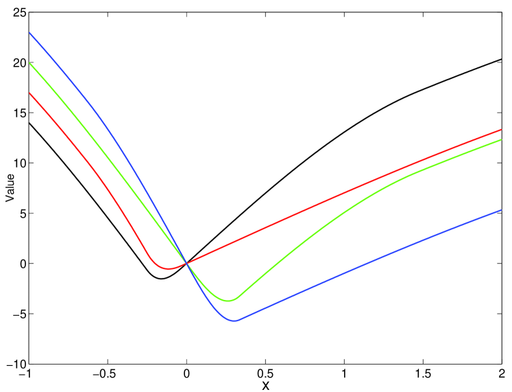
(a) $C(1,2)=2,C(2,1)=5,\chi(1,2)=2,\chi(2,1)=5$

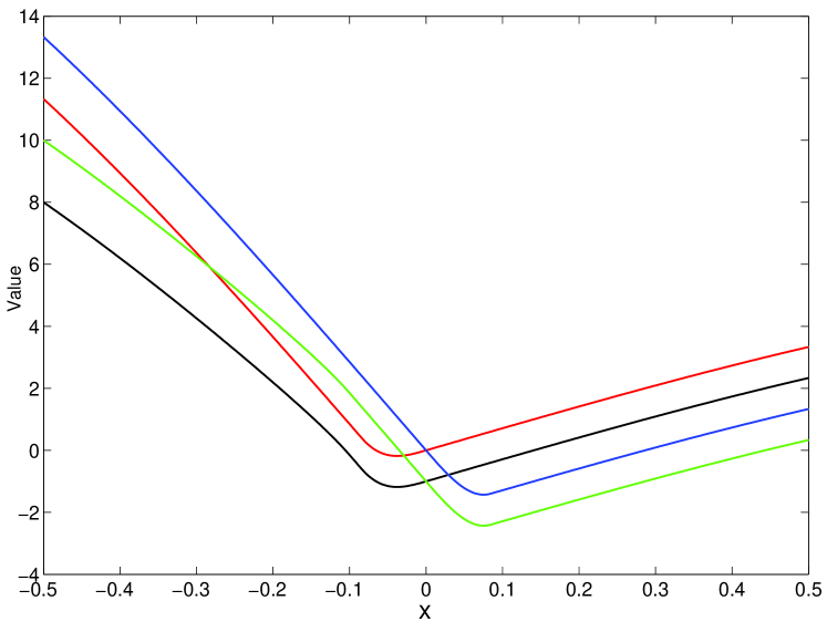
(b) $C(1,2)=5,C(2,1)=-1,\chi(1,2)=2,\chi(2,1)=2$

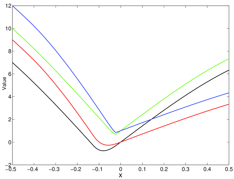
(c) $C(1,2)=2,C(2,1)=2,\chi(1,2)=-1,\chi(2,1)=5$

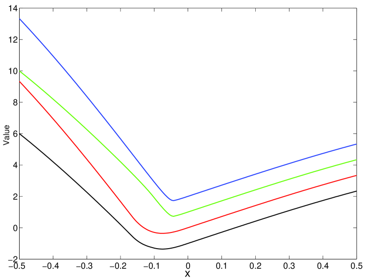
(d) $C(1,2)=4,C(2,1)=-2,\chi(1,2)=-1,\chi(2,1)=3$

Figure 1: Value functions:$V^{11}$(black),$V^{12}$(red),$V^{21}$(green),$V^{22}$(blue)

.

Next, we plot the optimal strategies of our zero-sum stochastic differential game. We focus on exemple $(a)$ in figure $1$ . First let $\mathcal{I}_{ij\to kl}=\{x\in\mathbb{R}:V^{ij}(x)=V^{kl}(x)-C(i,k)+\chi(j,l)\}$. Then by figure $1$ (exemple $(a))$ we get

$$\begin{array}[]{ll}\mathcal{I}_{11\to 21}=(-\infty,-0.25]\qquad\quad\mathcal{I}_{11\to 12}=[1.46,+\infty)\\ \mathcal{I}_{12\to 21}=(-\infty,-0.62]\qquad\quad\mathcal{I}_{12\to 22}=[-0.62,-0.25]\\ \mathcal{I}_{21\to 11}=[0.33,1.46]\qquad\quad\;\;\;\mathcal{I}_{21\to 12}=[1.46,+\infty)\\ \mathcal{I}_{22\to 21}=(-\infty,-0.62]\qquad\quad\mathcal{I}_{22\to 12}=[0.33,+\infty)\end{array}$$ (7.2)

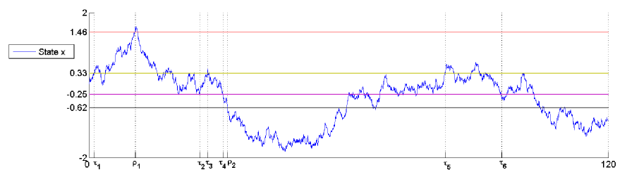
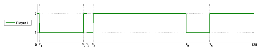
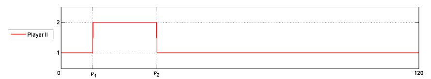
Figure 2: optimal strategies and state simulation

References

- [1] G. Barles : Solutions de Viscosité des équations de Hamilton-Jacobi. Mathématiques et Applications (17).Springer, Paris (1994).
- [2] R. Buckdahn and J. Li, Stochastic differential games and viscosity solutions of Hamilton– Jacobi-–Bellman–-Isaacs equations, SIAM J. Control Optim., 47 (2008), pp. 444–-475.
- [3] R. Carmona and M. Ludkovski: Valuation of energy storage: an optimal switching approach. Quant. Finance 10 (2010), no. 4, 359–374.
- [4] J.-F. Chassagneux, R. Elie and Kharroubi, I.: Discrete–time approximation of multi-dimensional BSDEs with oblique reflections. Ann. Appl. Probab. 22 (2012), no. 3, 971–1007.
- [5] M. Crandall, H. Ishii, H and P.L. Lions, User’s guide to viscosity solutions of second order partial differential equations, Bull. Amer. Math. Soc, 27 (1992), 1–67.
- [6] B. Djehiche, S. Hamadène, and M.-A. Morlais : Viscosity Solutions of Systems of Variational Inequalities with Inter-connected Bilateral Obstacles. Funkcialaj Ekvacioj, 58 (2015), pp.135–175.
- [7] B. Djehiche, S. Hamadène, and A. Popier: A finite horizon optimal multiple switching problem, SIAM Journal Control and Optim, 48(4): 2751–2770, 2009.
- [8] B. Djehiche, S. Hamadène, M.-A. Morlais, X. Zhao: On the equality of solutions of max–min and min–max systems of variational inequalities with interconnected bilateral obstacles. J. Math. Anal. Appl. 452(1), 148–175 (2017)
- [9] B. El Asri Deterministic minimax impulse control in finite horizon: the viscosity solution approach. ESAIM: Control Optim. Calc. Var., 19, 63–77.
- [10] B. El Asri Minimax Impulse Control Problems in Finite Horizon. arXiv:1305.0914
- [11] B. EL Asri and S. Mazid: Zero-sum stochastic differential game in finite horizon involving impulse controls. IN arxiv preprint arxiv: 1706.08880 (2017).
- [12] R. Elie and I. Kharroubi: Probabilistic representation and approximation for coupled systems of variational inequal-ities. Statist. Probab. Lett. 80 (2010), no. 17-18, 13881396.
- [13] R. Elliott and N. Kalton, The Existence of Value in Differential Games, Mem. Amer. Math. Soc. , American Mathematical Society, Providence, RI, .
- [14] C. Evans and E. Souganidis. Differential games and representation formulas for solutions of Hamilton-Jacobi-Isaacs equations. Indiana Univ. Math. J., 33(5):773-–797, 1984.
- [15] W. H. Fleming and P. E. Souganidis, On the existence of value functions of two-player, zero-sum stochastic differential games, Indiana Univ. Math. J., , pp. 293–314.
- [16] S. Hamadène and M. Jeanblanc,: On the starting and stopping problem: application in reversible investments. Math. Oper. Res. 32 (2007), no. 1, 182–192.
- [17] S. Hamadène and J.-P. Lepeltier, Zero-sum stochastic differential games and backward equations, Systems Control Lett., 24 (1995), pp. 259–-263.
- [18] S. Hamadène, J.-P. Lepeltier, and S. Peng, BSDEs with continuous coefficients and stochastic differential games. in Backward Stochastic Differential Equations, N. El Karoui and L. Mazliak eds., Pitman Res. Notes Math. Ser., 364, Longman, Harlow (1997), pp. 115–-128.
- [19] Y. Hu and S. Tang: Multi-dimensional BSDE with oblique reflection and optimal switching, Proba. Theo. and Rel. Fields, 147, N. 1-2: 89–121, 2010.
- [20] H. Ishii and S.Koike: Viscosity Solutions of a System of Nonlinear Second-Order Elliptic PDEs Arising in Switching Games. Funkcialaj Ekvacioj, 34 (1991) 143-155.
- [21] R. Isaacs. Differential games. A mathematical theory with applications to warfare and pursuit, control and optimization. John Wiley and Sons, Inc., New York-London-Sydney, 1965.
- [22] M. Ludkovski: Stochastic switching games and duopolistic competition in emissions markets. SIAM J. Financial Math. 2 (2011), no. 1, 488–511.
- [23] K. Li, K. Nystrom and M.Olofsson: Optimal switching problems under partial information. Monte Carlo Methods and Applications, 21(2), 91-120 (2015).
- [24] N.L.P. Lundstrom, K. Nystrom and M. Olofsson: Systems of variational inequalities in the context of optimal switching problems and operators of Kolmogorov type. Annali di Matematica Pura ed Applicata (2014) Volume 193, Issue 4, pp 1213–1247.
- [25] N.L.P. Lundstrom, K. Nystrom and M. Olofsson: Systems of Variational Inequalities for Non-Local Operators Related to Optimal Switching Problems: Existence and Uniqueness. Manuscripta Mathematica, Nov. 2014, Vol. 145, Issue 3, pp. 407–432.
- [26] V. Ly Vath and H. Pham, Explicit solution to an optimal switching problem in the two-regime case, SIAM J. Control Optim., 46 (2007), pp. 395–-426.
- [27] M. Perninge and L. Soder: Irreversible investments with delayed reaction: an application to generation re-dispatch in power system operation. Math. Methods Oper. Res. 79 (2014), no. 2, 195–224.
- [28] H. Pham, L.V. Vathana and X.Y.Zhou: Optimal switching over multiple regimes. SIAM J. Control Optim. 48 (2009), no. 4, 2217–2253.
- [29] D. Revuz and M. Yor, (1991): Continuous Martingales and Brownian Motion. Springer Verlag, Berlin.
- [30] S. Tang and S.-H. Hou : Switching games of stochastic differential systems, SIAM J. Control Optim., 46(3): 900–929, 2007.
- [31] L.C.G. Rogers and D. Williams, Diffusions, Markov processes, and martingales. John Wiley and Sons, New York (1987).
- [32] S. Tang and S.-H. Hou : Switching games of stochastic differential systems, SIAM J. Control Optim., 46(3): 900–-929, 2007.
- [33] S. Tang and J. Yong (1993) : Finite horizon stochastic optimal switching and impulse controls with a viscosity solution approachâ€, Stoch. and Stoch. Reports, 45, 145–176.
- [34] M. Zervos : A problem of sequential entry and exit decisions combined with discretionary stopping. SIAM J. Control Optim. 42 (2003), no. 2, 397-421 (electronic).