The Algorithm Selection Competitions 2015 and 2017

Abstract

The algorithm selection problem is to choose the most suitable algorithm for solving a given problem instance. It leverages the complementarity between different approaches that is present in many areas of AI. We report on the state of the art in algorithm selection, as defined by the Algorithm Selection competitions in 2015 and 2017. The results of these competitions show how the state of the art improved over the years. We show that although performance in some cases is very good, there is still room for improvement in other cases. Finally, we provide insights into why some scenarios are hard, and pose challenges to the community on how to advance the current state of the art.

1 Introduction

In many areas of AI, there are different algorithms to solve the same type of problem. Often, these algorithms are complementary in the sense that one algorithm works well when others fail and vice versa. For example in propositional satisfiability solving (SAT), there are complete tree-based solvers aimed at structured, industrial-like problems, and local search solvers aimed at randomly generated problems. In many practical cases, the performance difference between algorithms can be very large, for example as shown by Xu et al. (2012) for SAT. Unfortunately, the correct selection of an algorithm is not always as easy as described above and even easy decisions require substantial expert knowledge about algorithms and the problem instances at hand.

Per-instance algorithm selection (Rice, 1976) is a way to leverage this complementarity between different algorithms. Instead of running a single algorithm, a portfolio (Huberman et al., 1997; Gomes and Selman, 2001) consisting of several complementary algorithms is employed together with a learned selector. The selector automatically chooses the best algorithm from the portfolio for each instance to be solved.

Formally, the task is to select the best algorithm $\mathbf{A}$ from a portfolio of algorithms $\mathcal{P}$ for a given instance $i$ from a set of instances $\mathcal{I}$ with respect to a performance metric $m:\mathcal{P}\times\mathcal{I}\to\mathbb{R}$ (e.g., runtime, error, solution quality or accuracy). To this end, an algorithm selection system learns a mapping from an instance to a selected algorithm $s:\mathcal{I}\to\mathcal{P}$ such that the performance, measured as cost, across all instances $\mathcal{I}$ is minimized (w.l.o.g.):

$$\operatorname*{arg\,min}_{s}\sum_{i\in\mathcal{I}}m(s(i),i)$$ (1)

Algorithm selection has gained prominence in many areas and made tremendous progress in recent years. Algorithm selection systems established new state-of-the-art performance in several areas of AI, for example propositional satisfiability solving (Xu et al., 2008), machine learning (Brazdil et al., 2008; van Rijn et al., 2018), maximum satisfiability solving (Ansótegui et al., 2016), answer set programming (Lindauer et al., 2017a; Calimeri et al., 2017), constraint programming (Hurley et al., 2014; Amadini et al., 2014), and the traveling salesperson problem (Kotthoff et al., 2015). However, the multitude of different approaches and application domains makes it difficult to compare different algorithm selection systems, which presented users with a very practical meta-algorithm selection problem – which algorithm selection system should be used for a given task. The algorithm selection competitions can help users to make the decision which system and approach to use, based on a fair comparison across a diverse range of different domains.

The first step towards being able to perform such comparisons was the introduction of the Algorithm Selection Benchmark Library (ASlib, Bischl et al., 2016). ASlib consists of many algorithm selection scenarios for which performance data of all algorithms on all instances is available. These scenarios allow for fair and reproducible comparisons of different algorithm selection systems. ASlib enabled the competitions we report on here.

Structure of the paper

In this competition report, we summarize the results and insights gained by running two algorithm selection competitions based on ASlib. These competitions were organized in 2015 – the ICON Challenge on Algorithm Selection – and in 2017 – the Open Algorithm Selection Challenge. We start by giving a brief background on algorithm selection (Section 2) and an overview on how we designed both competitions (Section 3). Afterwards we present the results of both competitions (Section 4) and discuss the insights obtained and open challenges in the field of algorithm selection, identified through the competitions (Section 5).

2 Background on Algorithm Selection

In this section, we discuss the importance of algorithm selection, several classes of algorithm selection methods and ways to evaluate algorithm selection problems.

2.1 Importance of Algorithm Selection

The impact of algorithm selection in several AI fields is best illustrated by the performance of such approaches in AI competitions. One of the first well-know algorithm selection systems was SATzilla (Xu et al., 2008), which won several first places in the SAT competition 2009 and the SAT challenge 2012. To refocus on core SAT solvers, portfolio solvers (including algorithm selection systems) were banned from the SAT competition for several years—now, they are allowed in a special track. In the answer set competition 2011, the algorithm selection system claspfolio (Hoos et al., 2014) won the NP-track and later in 2015, ME-ASP (Maratea et al., 2015) won the competition. In constraint programming, sunny-cp (Amadini et al., 2014) won the open track of the MiniZinc Challenge for several years (2015, 2016 & 2017). In AI planning, a simple static portfolio of planners (fast downward stone soup; Helmert et al., 2011) won a track at the International Planning Competition (IPC) in 2011. More recently, the online algorithm selection system Delfi (Katz et al., 2018) won a first place at IPC 2018. In QBF, an algorithm selection system called QBF Portfolio (Hoos et al., 2018) won third place at the prenex track of QBFEVAL 2018.

Algorithm selection does not only perform well for combinatorial problems, but it is also an important component in automated machine learning (AutoML) systems. For example, the AutoML system auto-sklearn uses algorithm selection to initialize its hyperparameter optimization (Feurer et al., 2015b) and won two AutoML challenges Feurer et al. (2018).

There are also applications of algorithm selection in non-AI domains, e.g. diagnosis (Koitz and Wotawa, 2016), databases (Dutt and Haritsa, 2016), and network design (Selvaraj and Nagarajan, 2017).

2.2 Algorithm Selection Approaches

Figure 1: Per-instance algorithm selection workflow for a given instance.

Figure 1 shows a basic per-instance algorithm selection framework that is used in practice. A basic approach involves (i) representing a given instance $i$ with a vector of numerical features $\mathcal{F}(i)$ (e.g., number of variables and constraints of a CSP instance), (ii) inducing a selection machine learning model $s$ that selects an algorithm for the given instance $i$ based on its features $\mathcal{F}(i)$. Generally, these machine learning models are induced based on a dataset $\mathcal{D}=\{(\mathbf{x}_{j},y_{j})\mid j=1,\ldots,n\}$ with $n$ datapoints to map an input $\mathbf{x}$ to output $f(\mathbf{x})$, which closely represents $y$. In this setting, $\mathbf{x}_{i}$ is typically the vector of numerical features $\mathcal{F}(i)$ from some instance $i$ that has been observed before. There are various variations for representing the $y$ values and ways for algorithm selection system $s$ to leverage the predictions $f(\mathbf{x})$. We briefly review several classes of solutions.

Regression

that models the performance of individual algorithms in the portfolio. A regression model $f_{\mathbf{A}}$ can be trained for each $\mathbf{A}\in\mathcal{P}$ on $\mathcal{D}$ with $\mathbf{x}_{j}=\mathcal{F}(i)$ and $y_{j}=m(\mathbf{A},i)$ for each previously observed instance $i$ that $\mathbf{A}$ was ran on. The machine learning algorithm can then predict how well algorithm $\mathbf{A}$ performs on a given instance from $\mathcal{I}$. The algorithm with the best predicted performance is selected for solving the instance (e.g., Horvitz et al., 2001; Xu et al., 2008).

Combinations of unsupervised clustering and classification

that partitions instances into clusters $H$ based on the instance features $\mathcal{F}(i)$, and determines the best algorithm $\mathbf{A}_{i}$ for each cluster $h_{i}\in H$. Given a new instance $i^{\prime}$, the instance features $\mathcal{F}(i^{\prime})$ determine the nearest cluster $h^{\prime}$ w.r.t. some distance metric; the algorithm $\mathbf{A}^{\prime}$ assigned to $h^{\prime}$ is applied (e.g., Ansótegui et al., 2009).

Pairwise Classification

that considers pairs of algorithms $(\mathbf{A}_{k},\mathbf{A}_{j})$. For a new instance, the machine-learning-induced model predicts for each pair of algorithms which one will perform better ($m(\mathbf{A}_{k},i)<m(\mathbf{A}_{j},i)$), and the algorithm with most “is better” predictions is selected (e.g., Xu et al., 2011; van Rijn et al., 2015).

Stacking of several approaches

that combine multiple models to predict the algorithm to choose, for example by predicting the performance of each portfolio algorithm through regression models and combining these predictions through a classification model (e.g., Kotthoff, 2012; Samulowitz et al., 2013; Malone et al., 2018).

2.3 Why is algorithm selection more than traditional machine learning?

In contrast to typical machine learning tasks, each instance has a weight attached to it. It is not be important to select the best algorithm on instances on which all algorithms perform nearly equally, but it is crucial to select the best algorithm on an instance on which all but one algorithm perform poorly (e.g., all but one time out). The potential gain from making the best decision can be seen as a weight for that particular instance.

Instead of predicting a single algorithm, schedules of algorithms can also be used. One variant of algorithm schedules (Kadioglu et al., 2011; Hoos et al., 2015) are static (instance-independent) pre-solving schedules which are applied before any instance features are computed (Xu et al., 2008). Computing the best-performing schedule is usually an NP-hard problem. Alternatively, a sequence of algorithms can be predicted for instance-specific schedules (Amadini et al., 2014; Lindauer et al., 2016).

Computing instance features can come with a large amount of overhead, and if the objective is to minimize runtime, this overhead should be minimized. For example, on industrial-like SAT instances, computing some instance features can take more than half of the total time budget.

For more details on algorithm selection systems and the different approaches used in the literature, we refer the interested reader to the surveys by Smith-Miles (2008) and Kotthoff (2014).

2.4 Evaluation of Algorithm Selection Systems

The purpose of performing algorithm selection is to achieve performance better than any individual algorithm could. In many cases, overhead through the computation of the instance features used as input for the machine learning models is incurred. This diminishes performance gains achieved through selecting good algorithms and has to be taken into account for evaluating algorithm selection systems.

To be able to assess the performance gain of algorithm selection systems, two baselines are commonly compared against (Xu et al., 2012; Lindauer et al., 2015; Ansótegui et al., 2016): (i) the performance of the individual algorithm performing best on all training instances (called single best solver (SBS)), which denotes what can be achieved without algorithm selection; (ii) the performance of the virtual best solver (VBS) (also called oracle performance), which makes perfect decisions and chooses the best-performing algorithm on each instance without any overhead. The VBS corresponds to the overhead-free parallel portfolio that runs all algorithms in parallel and terminates as soon as the first algorithm finishes.

The performance of the baselines and of any algorithm selection system varies for different scenarios. We normalize the performance $m_{s}=\sum_{i\in\mathcal{I}}m(s(i),i)$ of an algorithm selection system $s$ on a given scenario by the performance of the SBS and VBS, as a cost to be minimized, and measure how much of the gap between the two it closed as follows:

$$\hat{m}_{s}=\frac{m_{s}-m_{VBS}}{m_{SBS}-m_{VBS}}$$ (2)

where $0$ corresponds to perfect performance, equivalent to the VBS, and $1$ corresponds to the performance of the SBS. The performance of an algorithm selection system will usually be between 0 and 1; if it is larger than 1 it means that simply always selecting the SBS is a better strategy.

A common way of measuring runtime performance is penalized average runtime (PAR10) (Hutter et al., 2014; Lindauer et al., 2015; Ansótegui et al., 2016): the average runtime across all instances, where algorithms are run with a timeout and penalized with a runtime ten times the timeout if they do not complete within the time limit.

3 Competition Setups

In this section, we discuss the setups of both competitions. Both competitions were based on ASlib, with submissions required to read the ASlib format as input.

3.1 General Setup: ASlib

Figure 2 shows the general structure of an ASlib scenario (Bischl et al., 2016). ASlib scenarios contain pre-computed performance values $m(\mathbf{A},i)$ for all algorithms in a portfolio $\mathbf{A}\in\mathcal{P}$ on a set of training instances $i\in\mathcal{I}$ (e.g., runtime for SAT instances or accuracy for Machine Learning datasets). In addition, a set of pre-computed instance features $\mathcal{F}(i)$ are available for each instance, as well as the time required to compute the feature values (the overhead). The corresponding task description provides further information, e.g., runtime cutoff, grouping of features, performance metric (runtime or solution quality) and indicates whether the performance metric is to be maximized or minimized. Finally, it contains a file describing the train-test splits. This file specifies which instances should be used for training the system ($\mathcal{I}_{Train}$), and which should be used for evaluating the system ($\mathcal{I}_{Test}$).

Figure 2: Illustration of ASlib.

3.2 Competition 2015

In 2015, the competition asked for complete systems to be submitted which would be trained and evaluated by the organizers. This way, the general applicability of submissions was emphasized – rather than doing well only with specific models and after manual tweaks, submissions had to demonstrate that they can be used off-the-shelf to produce algorithm selection models with good performance. For this reason, submissions were required to be open source or free for academic use.

The scenarios used in 2015 are shown in Table 1. The competition used existing ASlib scenarios that were known to the participants beforehand. There was no secret test data in 2015; however, the splits into training and testing data were not known to participants. We note that these are all runtime scenarios, reflecting what was available in ASlib at the time.

Submissions were allowed to specify the feature groups and a single pre-solver for each ASlib scenario (a statically-defined algorithm to be run before any feature computation to avoid overheads on easy instances), and required to produce a list of the algorithms to run for each instance (each with an associated timeout). The training time for a submission was limited to $12$ CPU hours on each scenario; each submission had the same computational resources available and was executed on the same hardware. AutoFolio was the only submission that used the full $12$ hours. The submissions were evaluated on $10$ different train-test splits, to reduce the potential influence of randomness. We considered the three metrics mean PAR10 score, mean misclassification penalty (the additional time that was required to solve an instance compared to the best algorithm on that instance), and number of instances solved within the timeout. The final score was the average remaining gap $\hat{m}$ (Equation 2) across these three metrics, the $10$ train-test splits, and the scenarios.

Scenario	$|\mathbf{A}|$	$|\mathcal{I}|$	$|\mathcal{F}|$	Obj.	Factor
ASP-POTASSCO	$11$	$1294$	$138$	Time	$25$
CSP-2010	$2$	$2024$	$17$	Time	$10$
MAXSAT12-PMS	$6$	$876$	$37$	Time	$53$
CPMP-2013	$4$	$527$	$22$	Time	$31$
PROTEUS-2014	$22$	$4021$	$198$	Time	$413$
QBF-2011	$5$	$1368$	$46$	Time	$96$
SAT11-HAND	$15$	$296$	$115$	Time	$37$
SAT11-INDU	$18$	$300$	$115$	Time	$22$
SAT11-RAND	$9$	$600$	$115$	Time	$66$
SAT12-ALL	$31$	$1614$	$115$	Time	$30$
SAT12-HAND	$31$	$1167$	$138$	Time	$35$
SAT12-INDU	$31$	$767$	$138$	Time	$15$
SAT12-RAND	$31$	$1167$	$138$	Time	$12$

Table 1: Overview of algorithm selection scenarios used in 2015, showing the number of algorithms $|\mathbf{A}|$, the number of instances $|\mathcal{I}|$, the number of instance features $|\mathcal{F}|$, the performance objective, and the improvement factor of the virtual best solver (VBS) over the single best solver $\left(m_{\textit{SBS}}/m_{\textit{VBS}}\right)$ without considering instances on which all algorithms timed out.

3.3 Competition 2017

Scenario	Alias	$|\mathbf{A}|$	$|\mathcal{I}|$	$|\mathcal{F}|$	Obj.	Factor
BNSL-2016∗	Bado	$8$	$1179$	$86$	Time	$41$
CSP-Minizinc-Obj-2016	Camilla	$8$	$100$	$95$	Quality	$1.7$
CSP-Minizinc-Time-2016	Caren	$8$	$100$	$95$	Time	$61$
MAXSAT-PMS-2016	Magnus	$19$	$601$	$37$	Time	$25$
MAXSAT-WPMS-2016	Monty	$18$	$630$	$37$	Time	$16$
MIP-2016	Mira	$5$	$218$	$143$	Time	$11$
OPENML-WEKA-2017	Oberon	$30$	$105$	$103$	Quality	$1.02$
QBF-2016	Qill	$24$	$825$	$46$	Time	$265$
SAT12-ALL∗	Svea	$31$	$1614$	$115$	Time	$30$
SAT03-16_INDU	Sora	$10$	$2000$	$483$	Time	$13$
TTP-2016∗	Titus	$22$	$9720$	$50$	Quality	$1.04$

Table 2: Overview of algorithm selection scenarios used in 2017, showing the alias in the competition, the number of algorithms $|\mathbf{A}|$, the number of instances $|\mathcal{I}|$, the number of instance features $|\mathcal{F}|$, the performance objective, and the improvement factor of the virtual best solver (VBS) over the single best solver $\left(m_{\textit{SBS}}/m_{\textit{VBS}}\right)$ without considering instances on which all algorithms timed out. Scenarios marked with an asterisk were available in ASlib before the competition.

Compared to 2015, we changed the setup of the competition in 2017 with the following goals in mind:

1. fewer restrictions on the submissions regarding computational resources and licensing;

2. better scaling of the organizational overhead to more submissions, in particular not having to run each submission manually;

3. more flexible schedules for computing features and running algorithms; and

4. a more diverse set of algorithm selection scenarios, including new scenarios.

To achieve the first and second goal, the participants did not submit their systems directly, but only the predictions made by their system for new test instances (using a single train-test split). Thus, also submissions from closed-source systems were possible, although all participants made their submissions open-source in the end. We provided full information, including algorithms’ performances, for a set of training instances, but only the feature values for the test instances to submitters. Participants could invest as many computational resources as they wanted to compute their predictions. While this may give an advantage to participants who have access to large amounts of computational resources, such a competition is typically won through better ideas and not through better computational resources. To facilitate easy submission of results, we did not run multiple train-test splits as in 2015. We be briefly investigated the effects of this in Section 5.4. We note that this setup is quite common in other machine learning competitions, e.g., the Kaggle competitions (Carpenter, 2011).

To support more complex algorithm selection approaches, the submitted predictions were allowed to be an arbitrary sequence of algorithms with timeouts and interleaved feature computations. Thus, any combination of these two components was possible (e.g., complex pre-solving schedules with interleaved feature computation). Complex pre-solving schedules were used by most submissions for scenarios with runtime as performance metric.

We collected several new algorithm selection benchmarks from different domains; $8$ out of the $11$ used scenarios were completely new and not disclosed to participants before the competition (see Table 2). We obfuscated the instance and algorithm names such that the participants were not able to easily recognize existing scenarios.

To show the impact of algorithm selection on the state of the art in different domains, we focused the search for new scenarios on recent competitions for CSP, MAXSAT, MIP, QBF, and SAT. Additionally, we developed an open-source Python tool that connects to OpenML (Vanschoren et al., 2014) and converts a Machine Learning study into an ASlib scenario. To ensure diversity of the scenarios with respect to the application domains, we selected at most two scenarios from each domain to avoid any bias introduced by focusing on a single domain. In the 2015 competition, most of the scenarios came from SAT, which skewed the evaluation in favor of that. Finally, we also considered scenarios with solution quality as performance metric (instead of runtime) for the first time. The new scenarios were added to ASlib after the competition; thus the competition was not only enabled by ASlib, but furthers its expansion.

For a detailed description of the competition setup in 2017, we refer the interested reader to Lindauer et al. (2017b).

4 Results

We now discuss the results of both competitions.

4.1 Competition 2015

The competition received a total of 8 submissions from 4 different groups of researchers comprising 15 people. Participants were based in 4 different countries on 2 continents. A provides an overview of all submissions.

Rank	System	Avg. Gap
		All	PAR10
1st	zilla	0.366	0.344
2nd	zillafolio	0.370	0.341
ooc	AutoFolio-48	0.375	0.334
3rd	AutoFolio	0.390	0.341
ooc	LLAMA-regrPairs	0.395	0.375
4th	ASAP_RF	0.416	0.377
5th	ASAP_kNN	0.423	0.387
ooc	LLAMA-regr	0.425	0.407
6th	flexfolio-schedules	0.442	0.395
7th	sunny	0.482	0.461
8th	sunny-presolv	0.484	0.467

Table 3: Results in 2015 with some system running out of competition (ooc). The average gap is aggregated across all scenarios according to Equation 2.

Table 3 shows the final ranking. The zilla system is the overall winner, although the first- and second-placed entries are very close. All systems perform well on average, closing more than half of the gap between virtual and single best solver. Additionally, we show the normalized PAR10 score for comparison to the 2017 results, where only the PAR10 metric was used. Detailed results of all metrics (PAR10, misclassification penalty, and solved) are presented in D.

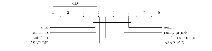
Figure 3: Critical distance plots with Nemenyi Test on the ‘All’ scores (average across normalized scores based on PAR10, misclassification penalty, and number of solved instances) of the participants of the 2015 competition. If two submissions are connected by a thick line, there was not enough statistical evidence that their performances are significantly different.

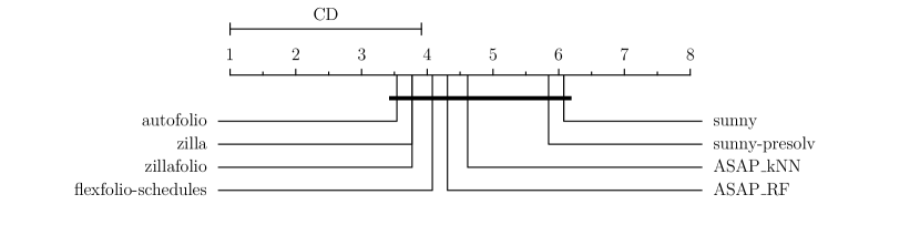
Figure 4: Critical distance plots with Nemenyi Test on the PAR10 scores of the participants of the 2015 competition.

For comparison, we show three additional systems. Autofolio-48 is identical to Autofolio (a submitted algorithm selector that searches over different selection approaches and their hyperparameter settings (Lindauer et al., 2015)), but was allowed $48$ hours training time (four times the default) to assess the impact of additional tuning of hyperparameters. LLAMA-regrPairs and LLAMA-regr are simple approaches based on the LLAMA algorithm selection toolkit (Kotthoff, 2013). The relatively small difference between AutoFolio and AutoFolio-48 shows that allowing more training time does not increase performance significantly. The good ranking of the two simple LLAMA models shows that reasonable performance can be achieved even with simple off-the-shelf approaches without customization or tuning. Figure 3 (combined scores) and Figure 4 (PAR10 scores) show critical distance plots on the average ranks of the submissions. According to the Friedman test with post-hoc Nemenyi test, there is no statistically significant difference between any of the submissions.

More detailed results can be found in Kotthoff (2015).

4.2 Competition 2017

In 2017, there were $8$ submissions from $4$ groups. Similar to 2015, participants were based in 4 different countries on 2 continents. While most of the submissions came from participants of the 2015 competition, there were also submissions by researchers who did not participate in 2015.

Rank	System	Avg. Gap	Avg. Rank
1st	ASAP.v2	$0.38$	$2.6$
2nd	ASAP.v3	$0.40$	$2.8$
3rd	Sunny-fkvar	$0.43$	$2.7$
4th	Sunny-autok	$0.57$	$3.9$
ooc	∗Zilla(fixed version)	$0.57$	N/A
5th	∗Zilla	$0.93$	$5.3$
6th	∗Zilla(dyn)	$0.96$	$5.4$
7th	AS-RF	$2.10$	$6.1$
8th	AS-ASL	$2.51$	$7.2$

Table 4: Results in 2017 with some system running out of competition (ooc). The average gap is aggregated across all scenarios according to Equation 2.

Table 4 shows the results in terms of the gap metric (see Equation 2) based on PAR10, as well as the ranks; detailed results are in Table 9 (E). The competition was won by ASAP.v2, which obtained the highest scores on the gap metric both in terms of the average over all datasets, and the average rank across all scenarios. Both ASAP systems clearly outperformed all other participants on the quality scenarios. However, Sunny-fkvar did best on the runtime scenarios, followed by ASAP.v2.

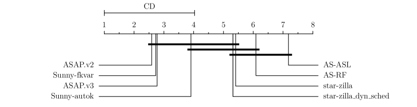
Figure 5: Critical distance plots with Nemenyi Test on the PAR10 scores of the participants in 2017.

Figure 5 shows critical distance plots on the average ranks of the submissions. There is no statistically significant difference between the best six submissions, but the difference to the worst submissions is statistically significant.

5 Open Challenges and Insights

In this section, we discuss insights and open challenges indicated by the results of the competitions.

5.1 Progress from 2015 to 2017

The progress of algorithm selection as a field from 2015 to 2017 seems to be rather small. In terms of the remaining gap between virtual best and single best solver, the results were nearly the same (the best system in 2015 achieved about $33\%$ in terms of PAR10, and the best system in 2017 about $38\%$). On the only scenario used in both competitions (SAT12-ALL), the performance stayed nearly constant. Nevertheless, the competition in 2017 was more challenging because of the new and more diverse scenarios. While the community succeeded in coming up with more challenging problems, there appears to be room for more innovative solutions.

5.2 Statistical Significance

Figures 3, 4 and 5 show ranked plots, with the critical distance required according to the Friedman with post-hoc Nemenyi test to assert statistical significant difference between multiple systems (Demsar, 2006). In the 2015 competition, none of the differences between the submitted systems were statistical significant, whereas in the 2017 competition only some differences where statistical significant.

Failure to detect a significant difference does not imply that there is no such difference: the statistical tests are based on a relatively low number of samples and thus have limited power.

Even though the statistical significance results should be interpreted with care, the critical difference plots are still informative. They show, e.g., that the systems submitted in the 2015 challenge were closer together (ranked approximately between $3.5$ and $6$) than the systems submitted in 2017 (ranked approximately between $2.5$ and $7$).

5.3 Robustness of Algorithm Selection Systems

As the results of both competitions show, choosing one of the state-of-the-art algorithm selection systems is still a much better choice than simply always using the single best algorithm. However, as different algorithm selection systems have different strengths, we are now confronted with a meta-algorithm selection problem – selecting the best algorithm selection approach for the task at hand. For example, while the best submission in 2017 achieved $38\%$ gap between SBS and VBS remaining, the virtual best selector over the portfolio of all submissions would have achieved $29\%$. An open challenge is to develop such a meta-algorithm selection system, or a single algorithm selection system that performs well across a wide range of scenarios.

One step in this direction is the per-scenario customization of the systems, e.g., by using hyperparameter optimization methods (Gonard et al., 2017; Liu et al., 2017; Cameron et al., 2017), per-scenario model selection (Malone et al., 2017), or even per-scenario selection of the general approach combined with hyperparameter optimization (Lindauer et al., 2015). However, as the results show, more fine-tuning of an algorithm selection system does not always result in a better-performing system. In 2015, giving much more time to Autofolio resulted in only a very minor performance improvement, and in 2017 ASAP.v2 performed better than its refined successor ASAP.v3.

In addition to the general observations above, we note the following points regarding robustness of the submissions:

• zilla performed very well on SAT scenarios (average rank: $1.4$) but only mediocre on other domains (average rank: $6.5$ out of $8$ submissions) in 2015;

• ASAP won in 2017, but sunny-fkvar performed better on runtime scenarios;

• both CSP scenarios in 2017 were very similar (same algorithm portfolio, same instances, same instance features) but the performance metric was changed (one scenario with runtime and one scenario with solution quality). On the runtime scenario, Sunny-fkvar performed very well, but on the quality scenario ASAP.v3/2 performed much better.

5.4 Impact of Randomness

One of the main differences between the 2015 and 2017 challenges was that in 2015, the submissions were evaluated on 10 cross-validation splits to determine the final ranking, whereas in 2017, only a single training-test split was used. While this greatly reduced the effort for the competition organizers, it increased the risk of a particular submission with randomized components getting lucky.

In general, our expectation for the performance of a submission is that it does not depend on randomness much, i.e., its performance does not vary significantly across different test sets or random seeds. On the other hand, as we observed in Section 5.3, achieving good performance across multiple scenarios is an issue.

To determine the effect of randomness on performance, we ran the competition winner, ASAP.v2, with different random seeds on the CSP-Minizinc-Obj-2016 (Camilla) scenario, where it performed particularly well. Figure 6 shows the cumulative distribution function of the performance across different random seeds. The probability of ASAP.v2 performing as good or better than it did is very low, suggesting that it did choose a lucky random seed.

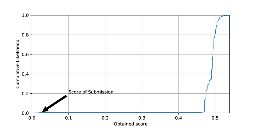
Figure 6: Cumulative distribution function of the closed gap of ASAP.v2 on CSP-Minizinc-Obj-2016, across 1500 random seeds. The plot shows that the actual obtained score ($0.025$) has a probability of $0.466\%$.

This result demonstrates the importance of evaluating algorithm selection systems across multiple random seeds, or multiple test sets. If we replace ASAP’s obtained score with the median score of the CDF shown in Figure 6, it would have ranked at third place.

5.5 Hyperparameter Optimization

All systems submitted to either of the competitions leverage a machine learning model that predicts the performance of algorithms. It is well known that hyperparameter optimization is important to get well-performing machine learning models (see, e.g., Snoek et al. (2012); Thornton et al. (2013); van Rijn and Hutter (2018)). Nevertheless, not all submissions optimized hyperparameters, e.g., the winner in 2017 ASAP.v2 (Gonard et al., 2017) used the default hyperparameters of its random forest. Given previous results by Lindauer et al. (2015), we would expect that adding hyperparameter optimization to recent algorithm selection systems will further boost their performances.

5.6 Handling of Quality Scenarios

ASlib distinguishes between two types of scenarios: runtime scenarios and quality scenarios. In runtime scenarios, the goal is to minimize the time the selected algorithm requires to solve an instances (e.g., SAT, ASP), whereas in quality scenarios the goal is to find the algorithm that obtains the highest score or lowest error according to some metric (e.g., plan quality in AI planning or prediction error in Machine Learning). In the current version of ASlib, the most important difference between the two scenario types is that for runtime scenario a schedule of different algorithms can be provided, whereas for quality scenarios only a single algorithm. The reason for this limitation is that ASlib does not contain information on intermediate solution qualities of any-time algorithms (e.g., the solution quality after half the timeout). For the same reason, the cost of feature computation cannot be considered for quality scenarios – it is unknown how much additional quality could be achieved in the time required for feature computation. This setup is common in algorithm selection methods for machine learning (meta-learning). Intermediate solutions and the time at which they were obtained could enable schedules for quality scenarios and analyzing trade-offs between obtaining a better solution quality by expending more resources or switching to another algorithm. For example, the MiniZinc Challenge (Stuckey et al., 2014) started to record these information in 2017. Future versions of ASlib will consider addressing this limitation.

5.7 Challenging Scenarios

Scenario	Median rem. gap	Best rem. gap
2015
ASP-POTASSCO	$0.31$	$0.28$
CSP-2010	$0.23$	$0.14$
MAXSAT12-PMS	$0.18$	$0.14$
CPMP-2013	$0.35$	$0.29$
PROTEUS-2014	$0.16$	$0.05$
QBF-2011	$0.15$	$0.09$
SAT11-HAND	$0.34$	$0.30$
SAT11-INDU	$1.00$	$\mathbf{0.87}$
SAT11-RAND	$0.08$	$0.04$
SAT12-ALL	$0.38$	$0.27$
SAT12-HAND	$0.32$	$0.25$
SAT12-INDU	$0.90$	$0.59$
SAT12-RAND	$1.00$	$\mathbf{0.77}$
Average	$0.41$	$0.31$
2017
BNSL-2016	$0.25$	$0.15$
CSP-Minizinc-Obj-2016	$1.59$	$0.02$
CSP-Minizinc-Time-2016	$0.41$	$0.05$
MAXSAT-PMS-2016	$0.49$	$0.41$
MAXSAT-WPMS-2016	$0.51$	$0.08$
MIP-2016	$0.56$	$0.49$
OPENML-WEKA-2017	$1.0$	$\mathbf{0.78}$
QBF-2016	$0.43$	$0.15$
SAT12-ALL	$0.42$	$0.31$
SAT03-16_INDU	$0.77$	$\mathbf{0.65}$
TTP-2016∗	$0.33$	$0.15$
Average	$0.61$	$0.30$

Table 5: Average remaining gap and the best remaining gap across all submissions for all scenarios. The bold scenarios are particularly challenging.

On average, algorithm selection systems perform well and the best systems had a remaining gap between the single best and virtual best solver of only $38\%$ in 2017. However, some of the scenarios are harder than others for algorithm selection. Table 5 shows the median and best performance of all submissions on all scenarios. To identify challenging scenarios, we studied the best-performing submission on each scenario and compared the remaining gap with the average remaining gap over all scenarios. In 2015, SAT12-RAND and SAT11-INDU were particularly challenging, and in 2017 OPENML-WEKA-2017 and SAT03-16_INDU.

SAT12-RAND

was a challenging scenario in 2015 and most of the participating systems performed not better than the single best solver on it, although the VBS has a 12-fold speedup over the single best solver. The main reason is probably that not only the SAT instances considered in this scenario are randomly generated but also most of the best-performing solvers are stochastic local search solvers which are highly randomized. The data in this scenario was obtained from single runs of each algorithm, which introduces strong noise. After the competition in 2015, Cameron et al. (2016) showed that in such noisy scenarios, the performance of the virtual best solver is often overestimated. Thus, we do not recommend to study algorithm selection on SAT12-RAND at this moment and plan to remove SAT12-RAND in the next ASlib release.

SAT11-INDU

was a hard scenario in 2015; in particular it was hard for systems that selected schedules per instance (such as Sunny). Applying schedules on these industrial-like instances is quite hard because even the single best solver has an average PAR10 score of $8030$ (with a timeout of $5000$ seconds) to solve an instance; thus, allocating a fraction of the total available resources to an algorithm on this scenario is often not a good idea (also shown by Hoos et al. (2015)).

SAT03-16_INDU

was a challenging scenario for the participants in $2017$. It is mainly an extension of a previously-used scenario called SAT12-INDU. Zilla was one of the best submissions in 2015 on SAT12-INDU with a remaining gap of roughly $61\%$; however in 2017 on SAT03-16_INDU, zilla had a remaining gap of $83\%$. Similar observations apply to ASAP. SAT03-16_INDU could be much harder than SAT12-INDU because of the smaller number of algorithms ($31\to 10$), the larger number of instances ($767\to 2000$) or the larger number of instance features ($138\to 483$).

OPENML-WEKA-2017

was a new scenario in the 2017 competition and appeared to be very challenging, as six out of eight submissions performed almost equal to or worse than the single best solver ($\geq 95\%$ remaining gap). This scenario featured algorithm selection for machine learning problems (cf. meta-learning (Brazdil et al., 2008)). The objective was to select the best machine learning algorithm from a selection of WEKA algorithms (Hall et al., 2009), based on simple characteristics of the dataset (i.e., meta-features). The scenario was introduced by van Rijn (2016)[Chapter 6]. We verified empirically that (i) there is a learnable concept in this scenario, and (ii) the chosen holdout set was sufficiently similar to the training data by evaluating a simple baseline algorithm selector (a regression approach using a random forest as model). The experimental setup and results are presented in Figure 7. It is indeed a challenging scenario; on half of the sampled holdout sets, our baseline was unable to close the gap by more than $10\%$. In $18\%$ of the holdout sets, the baseline performed worse than the SBS. However, our simple baseline achieved $67.5\%$ remaining gap on the holdout set used in the competition (compared to the best submission Sunny-fkvar with $78\%$).

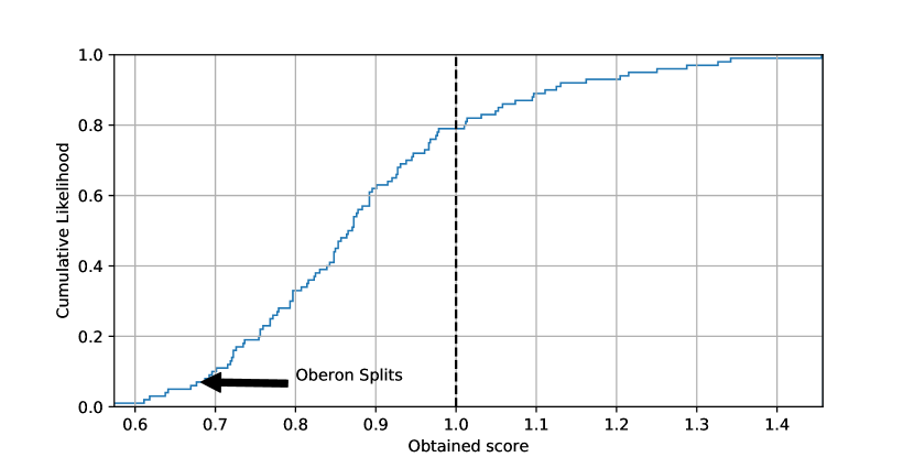
Figure 7: Cumulative distribution function of the obtained gap-remaining score of a random forest regressor (a single model trained to predict for all classifiers, 64 trees) on $100$ randomly sampled $33\%$ holdout sets of the OPENML-WEKA-2017 scenario. The dashed line indicates the performance of the single best solver; the score on the actual splits as presented in Oberon was $0.675$.

6 Conclusions

In this paper, we discussed the setup and results of two algorithm selection competitions. These competitions allow the community to objectively compare different systems and assess their benefits. They confirmed that per-instance algorithm selection can substantially improve the state of the art in many areas of AI. For example, the virtual best solver obtains on average a 31.8 fold speedup over the single best solver on the runtime scenarios from 2017. While the submissions fell short of this perfect performance, they did achieve significant improvements.

Perhaps more importantly, the competitions highlighted challenges for the community in a field that has been well-established for more than a decade. We identified several challenging scenarios on which the recent algorithm selection systems do not perform well. Furthermore, there is no system that performs well on all types of scenarios – a meta-algorithm selection problem is very much relevant in practice and warrants further research. The competitions also highlighted restrictions in the current version of ASlib, which enabled the competitions, that need to be addressed in future work.

References

Appendix A Submitted Systems in 2015

• ASAP based on random forests (RF) and $k$-nearest neighbor (kNN) as selection models combine pre-solving schedule and per-instance algorithm selection by training both jointly (Gonard et al., 2016).

• AutoFolio combines several algorithm selection approaches in a single systems and uses algorithm configuration (Hutter et al., 2011) to search for the best approach and its hyperparameter settings for the scenario at hand.

• Sunny selects an algorithm schedule on a per-instance base (Amadini et al., 2014). The time assigned to each algorithm is proportional to the number of solved instances in the neighborhood in the feature space with respect to the instance at hand.

• Zilla is the newest version of SATzilla (Xu et al., 2008, 2011) which uses pair-wise, cost-sensitive random forests combined with pre-solving schedules.

• ZillaFolio is a combination of Zilla and AutoFolio by evaluating both approaches on the training set and using the better approach for generating the predictions for the test set.

Appendix B Technical Evaluation Details in 2015

The evaluation was performed as follows. For each scenario, 10 bootstrap samples of the entire data were used to create 10 different train/test splits. No stratification was used. The training part was left unmodified. For the test part, algorithm performances were set to 0 and runstatus to “ok” for all algorithms and all instances – the ASlib specification requires algorithm performance data to be part of a scenario.

There was a time limit of 12 hours for the training phase. Systems that exceeded this limit were disqualified. The time limit was chosen for practical reasons, to make it possible to evaluate the submissions with reasonable resource requirements.

For systems that specified a pre-solver, the instances that were solved by the pre-solver within the specified time were removed from the training set. If a subset of features was specified, only these features (and only the costs associated with these features) were left in both training and test set, with all other feature values removed.

Each system was trained on each train scenario and predicted on each test scenario. In total, 130 evaluations (10 for each of the 13 scenarios) per submitted system were performed. The total CPU time spent was 4685.11 hours on 8-core Xeon E5-2640 CPUs.

Each system was evaluated in terms of mean PAR10 score, mean misclassification penalty (the additional time that was required to solve an instance because an algorithm that was not the best was chosen; the difference to the VBS), and mean number of instances solved for each of the 130 evaluations on each scenario and split. These are the same performance measures used in ASlib, and enable a direct comparison.

The final score of a submission group (i.e. a system submitted for different ASlib scenarios) was computed as the average score over all ASlib scenarios. For scenarios for which no system belonging to the group was submitted, the performance of the single best algorithm was assumed.

Appendix C Submitted Systems in 2017

• Gonard et al. (2017) submitted ASAP.v2 and ASAP.v3 (Gonard et al., 2016). ASAP combines pre-solving schedules and per-instance algorithm selection by training both jointly. The main difference between ASAP.v2 and ASAP.v3 is that ASAP.v2 used a pre-solving schedule with a fixed length of 3, whereas ASAP.v3 optimized the schedule length between 1 and 4 on a per-scenario base.

• Malone et al. (2017) submitted AS-RF and AS-ASL (Malone et al., 2018). It also combines pre-solving schedules and per-instance algorithm selection, whereas the selection model is a two-level stacking model with the first level being regression models to predict the performance of each algorithm and the second level combines these performance predictions in a multi-class model to obtain a selected algorithm. AS-RF uses random forest and AS-ASL used auto-sklearn (Feurer et al., 2015a) to obtain a machine learning model.

• Liu et al. (2017) submitted Sunny (autok and fkvar) (Amadini et al., 2014). Sunny selects per-instance algorithm schedules with the goal of minimizing the number of possible timeouts. Sunny-autok optimized the neighborhood size on a per-scenario base (Lindauer et al., 2016) and Sunny.fkvar additionally also applied greedy forward selection for instance feature subset selection.

• Cameron et al. (2017) submitted *Zilla (vanilla and dynamic), the successor of SATzilla (Xu et al., 2008, 2011). *Zilla also combines per-solving schedules and pre-instance algorithm selection but based on pair-wise weighted random forest models. The dynamic version of *Zilla additionally uses the trained random forest to extract a per-instance algorithm schedule.

Appendix D Detailed Results 2015 competition

scenario	zilla	zillafolio	autofolio	flexfolio-schedules
ASP-POTASSCO	$537$ ($5.0$)	$516$ ($1.0$)	$525$ ($3.0$)	$527$ ($4.0$)
CSP-2010	$6582$ ($4.0$)	$6549$ ($2.0$)	$6621$ ($7.0$)	$6573$ ($3.0$)
MAXSAT12-PMS	$3524$ ($6.0$)	$3598$ ($8.0$)	$3559$ ($7.0$)	$3375$ ($1.0$)
PREMARSHALLING-ASTAR-2013	$2599$ ($5.0$)	$2722$ ($7.0$)	$2482$ ($4.0$)	$2054$ ($2.0$)
PROTEUS-2014	$5324$ ($7.0$)	$5070$ ($5.0$)	$5057$ ($4.0$)	$4435$ ($1.0$)
QBF-2011	$9339$ ($7.0$)	$9366$ ($8.0$)	$9177$ ($6.0$)	$8653$ ($1.0$)
SAT11-HAND	$17436$ ($3.0$)	$17130$ ($1.0$)	$17746$ ($6.0$)	$17560$ ($4.0$)
SAT11-INDU	$13418$ ($3.0$)	$13768$ ($4.0$)	$13314$ ($1.0$)	$14560$ ($6.0$)
SAT11-RAND	$9495$ ($2.0$)	$9731$ ($3.0$)	$9428$ ($1.0$)	$10339$ ($8.0$)
SAT12-ALL	$964$ ($1.0$)	$1100$ ($3.0$)	$1066$ ($2.0$)	$1436$ ($6.0$)
SAT12-HAND	$4370$ ($2.0$)	$4432$ ($4.0$)	$4303$ ($1.0$)	$4602$ ($6.0$)
SAT12-INDU	$2754$ ($3.0$)	$2680$ ($1.0$)	$2688$ ($2.0$)	$2972$ ($4.0$)
SAT12-RAND	$3139$ ($1.0$)	$3146$ ($2.0$)	$3160$ ($3.0$)	$3240$ ($7.0$)
Average	$6114$ ($3.8$)	$6139$ ($3.8$)	$6087$ ($3.6$)	$6179$ ($4.1$)
scenario	ASAP_RF	ASAP_kNN	sunny	sunny-presolv
ASP-POTASSCO	$517$ ($2.0$)	$554$ ($7.0$)	$575$ ($8.0$)	$547$ ($6.0$)
CSP-2010	$6516$ ($1.0$)	$6601$ ($5.0$)	$6615$ ($6.0$)	$6704$ ($8.0$)
MAXSAT12-PMS	$3421$ ($3.0$)	$3395$ ($2.0$)	$3465$ ($4.0$)	$3521$ ($5.0$)
PREMARSHALLING-ASTAR-2013	$2660$ ($6.0$)	$2830$ ($8.0$)	$2151$ ($3.0$)	$1979$ ($1.0$)
PROTEUS-2014	$5169$ ($6.0$)	$5338$ ($8.0$)	$4866$ ($3.0$)	$4798$ ($2.0$)
QBF-2011	$8793$ ($2.0$)	$8813$ ($3.0$)	$8907$ ($4.0$)	$9044$ ($5.0$)
SAT11-HAND	$17581$ ($5.0$)	$17289$ ($2.0$)	$19130$ ($7.0$)	$19238$ ($8.0$)
SAT11-INDU	$13858$ ($5.0$)	$13359$ ($2.0$)	$14681$ ($7.0$)	$15160$ ($8.0$)
SAT11-RAND	$10018$ ($6.0$)	$9795$ ($4.0$)	$10212$ ($7.0$)	$9973$ ($5.0$)
SAT12-ALL	$1201$ ($5.0$)	$1181$ ($4.0$)	$1579$ ($7.0$)	$1661$ ($8.0$)
SAT12-HAND	$4434$ ($5.0$)	$4395$ ($3.0$)	$4823$ ($7.0$)	$4875$ ($8.0$)
SAT12-INDU	$3005$ ($6.0$)	$2974$ ($5.0$)	$3201$ ($8.0$)	$3173$ ($7.0$)
SAT12-RAND	$3211$ ($4.0$)	$3239$ ($6.0$)	$3263$ ($8.0$)	$3222$ ($5.0$)
Average	$6183$ ($4.3$)	$6136$ ($4.5$)	$6421$ ($6.1$)	$6453$ ($5.8$)

Table 6: Original results of the PAR10 scores of the 2015 competition.

scenario	zilla	zillafolio	autofolio	flexfolio-schedules
ASP-POTASSCO	$22$ ($5.0$)	$21$ ($2.0$)	$22$ ($3.0$)	$24$ ($7.0$)
CSP-2010	$14$ ($2.0$)	$11$ ($1.0$)	$28$ ($7.0$)	$23$ ($6.0$)
MAXSAT12-PMS	$38$ ($2.0$)	$42$ ($4.0$)	$177$ ($8.0$)	$41$ ($3.0$)
PREMARSHALLING-ASTAR-2013	$323$ ($5.0$)	$336$ ($7.0$)	$330$ ($6.0$)	$307$ ($4.0$)
PROTEUS-2014	$482$ ($8.0$)	$470$ ($7.0$)	$470$ ($6.0$)	$70$ ($1.0$)
QBF-2011	$192$ ($6.0$)	$194$ ($8.0$)	$182$ ($5.0$)	$133$ ($3.0$)
SAT11-HAND	$462$ ($3.0$)	$406$ ($1.0$)	$486$ ($5.0$)	$514$ ($6.0$)
SAT11-INDU	$615$ ($2.0$)	$639$ ($3.0$)	$574$ ($1.0$)	$779$ ($8.0$)
SAT11-RAND	$70$ ($3.0$)	$65$ ($2.0$)	$62$ ($1.0$)	$448$ ($8.0$)
SAT12-ALL	$95$ ($1.0$)	$111$ ($3.0$)	$103$ ($2.0$)	$211$ ($8.0$)
SAT12-HAND	$75$ ($1.0$)	$82$ ($3.0$)	$77$ ($2.0$)	$160$ ($8.0$)
SAT12-INDU	$87$ ($1.0$)	$100$ ($2.0$)	$103$ ($3.0$)	$139$ ($5.0$)
SAT12-RAND	$39$ ($1.0$)	$40$ ($2.0$)	$49$ ($4.0$)	$58$ ($5.0$)
Average	$194$ ($3.1$)	$194$ ($3.5$)	$205$ ($4.1$)	$224$ ($5.5$)
scenario	ASAP_RF	ASAP_kNN	sunny	sunny-presolv
ASP-POTASSCO	$23$ ($6.0$)	$25$ ($8.0$)	$20$ ($1.0$)	$22$ ($4.0$)
CSP-2010	$14$ ($3.0$)	$21$ ($4.0$)	$22$ ($5.0$)	$39$ ($8.0$)
MAXSAT12-PMS	$45$ ($6.0$)	$43$ ($5.0$)	$31$ ($1.0$)	$57$ ($7.0$)
PREMARSHALLING-ASTAR-2013	$271$ ($1.0$)	$275$ ($2.0$)	$338$ ($8.0$)	$296$ ($3.0$)
PROTEUS-2014	$235$ ($4.0$)	$249$ ($5.0$)	$224$ ($3.0$)	$136$ ($2.0$)
QBF-2011	$98$ ($2.0$)	$80$ ($1.0$)	$181$ ($4.0$)	$194$ ($7.0$)
SAT11-HAND	$466$ ($4.0$)	$431$ ($2.0$)	$634$ ($8.0$)	$618$ ($7.0$)
SAT11-INDU	$736$ ($6.0$)	$673$ ($4.0$)	$701$ ($5.0$)	$772$ ($7.0$)
SAT11-RAND	$124$ ($6.0$)	$129$ ($7.0$)	$122$ ($5.0$)	$85$ ($4.0$)
SAT12-ALL	$157$ ($5.0$)	$153$ ($4.0$)	$182$ ($6.0$)	$183$ ($7.0$)
SAT12-HAND	$114$ ($5.0$)	$102$ ($4.0$)	$124$ ($6.0$)	$129$ ($7.0$)
SAT12-INDU	$160$ ($8.0$)	$154$ ($7.0$)	$154$ ($6.0$)	$138$ ($4.0$)
SAT12-RAND	$60$ ($7.0$)	$67$ ($8.0$)	$58$ ($6.0$)	$45$ ($3.0$)
Average	$193$ ($4.8$)	$185$ ($4.7$)	$215$ ($4.9$)	$209$ ($5.4$)

Table 7: Original results of the misclassification penalty scores of the 2015 competition.

scenario	zilla	zillafolio	autofolio	flexfolio-schedules
ASP-POTASSCO	$0.915$ ($5.0$)	$0.919$ ($2.0$)	$0.917$ ($4.0$)	$0.918$ ($3.0$)
CSP-2010	$0.870$ ($4.0$)	$0.871$ ($2.0$)	$0.870$ ($6.0$)	$0.870$ ($3.0$)
MAXSAT12-PMS	$0.834$ ($7.0$)	$0.830$ ($8.0$)	$0.840$ ($4.0$)	$0.842$ ($1.0$)
PREMARSHALLING-ASTAR-2013	$0.937$ ($5.0$)	$0.933$ ($6.0$)	$0.940$ ($4.0$)	$0.953$ ($2.0$)
PROTEUS-2014	$0.863$ ($6.0$)	$0.871$ ($3.0$)	$0.871$ ($2.0$)	$0.878$ ($1.0$)
QBF-2011	$0.745$ ($7.0$)	$0.744$ ($8.0$)	$0.750$ ($6.0$)	$0.765$ ($1.0$)
SAT11-HAND	$0.659$ ($3.0$)	$0.665$ ($1.0$)	$0.653$ ($6.0$)	$0.658$ ($4.0$)
SAT11-INDU	$0.741$ ($3.0$)	$0.734$ ($5.0$)	$0.742$ ($2.0$)	$0.719$ ($6.0$)
SAT11-RAND	$0.815$ ($2.0$)	$0.809$ ($3.0$)	$0.816$ ($1.0$)	$0.804$ ($6.0$)
SAT12-ALL	$0.930$ ($1.0$)	$0.918$ ($3.0$)	$0.921$ ($2.0$)	$0.897$ ($6.0$)
SAT12-HAND	$0.643$ ($3.0$)	$0.638$ ($5.0$)	$0.649$ ($1.0$)	$0.629$ ($6.0$)
SAT12-INDU	$0.779$ ($3.0$)	$0.787$ ($1.0$)	$0.787$ ($2.0$)	$0.764$ ($5.0$)
SAT12-RAND	$0.742$ ($1.0$)	$0.742$ ($2.0$)	$0.741$ ($3.0$)	$0.735$ ($7.0$)
Average	$0.806$ ($3.8$)	$0.805$ ($3.8$)	$0.807$ ($3.3$)	$0.802$ ($3.9$)
scenario	ASAP_RF	ASAP_kNN	sunny	sunny-presolv
ASP-POTASSCO	$0.919$ ($1.0$)	$0.913$ ($7.0$)	$0.908$ ($8.0$)	$0.913$ ($6.0$)
CSP-2010	$0.872$ ($1.0$)	$0.870$ ($5.0$)	$0.870$ ($7.0$)	$0.868$ ($8.0$)
MAXSAT12-PMS	$0.840$ ($3.0$)	$0.841$ ($2.0$)	$0.837$ ($5.0$)	$0.835$ ($6.0$)
PREMARSHALLING-ASTAR-2013	$0.933$ ($7.0$)	$0.928$ ($8.0$)	$0.951$ ($3.0$)	$0.955$ ($1.0$)
PROTEUS-2014	$0.861$ ($7.0$)	$0.856$ ($8.0$)	$0.870$ ($4.0$)	$0.869$ ($5.0$)
QBF-2011	$0.759$ ($2.0$)	$0.758$ ($4.0$)	$0.758$ ($3.0$)	$0.754$ ($5.0$)
SAT11-HAND	$0.656$ ($5.0$)	$0.662$ ($2.0$)	$0.625$ ($7.0$)	$0.623$ ($8.0$)
SAT11-INDU	$0.734$ ($4.0$)	$0.744$ ($1.0$)	$0.715$ ($7.0$)	$0.706$ ($8.0$)
SAT11-RAND	$0.804$ ($7.0$)	$0.809$ ($4.0$)	$0.800$ ($8.0$)	$0.804$ ($5.0$)
SAT12-ALL	$0.913$ ($5.0$)	$0.915$ ($4.0$)	$0.881$ ($7.0$)	$0.873$ ($8.0$)
SAT12-HAND	$0.640$ ($4.0$)	$0.643$ ($2.0$)	$0.605$ ($7.0$)	$0.601$ ($8.0$)
SAT12-INDU	$0.763$ ($6.0$)	$0.765$ ($4.0$)	$0.744$ ($8.0$)	$0.745$ ($7.0$)
SAT12-RAND	$0.738$ ($4.0$)	$0.736$ ($5.0$)	$0.733$ ($8.0$)	$0.735$ ($6.0$)
Average	$0.802$ ($4.3$)	$0.803$ ($4.3$)	$0.792$ ($6.3$)	$0.791$ ($6.2$)

Table 8: Original results of the solved scores of the 2015 competition.

Appendix E Detailed Results 2017 competition

scenario	ASAP.v2	ASAP.v3	Sunny-fkvar	Sunny-autok
Bado	$0.239$ ($4.0$)	$0.192$ ($3.0$)	$0.153$ ($1.0$)	$0.252$ ($5.0$)
Camilla	$0.025$ ($1.5$)	$0.025$ ($1.5$)	$0.894$ ($3.0$)	$1.475$ ($4.0$)
Caren	$0.412$ ($5.0$)	$0.410$ ($4.0$)	$0.055$ ($1.0$)	$0.217$ ($2.0$)
Magnus	$0.492$ ($4.0$)	$0.494$ ($5.0$)	$0.419$ ($3.0$)	$0.498$ ($6.0$)
Mira	$0.495$ ($2.0$)	$0.491$ ($1.0$)	$0.568$ ($4.0$)	$1.014$ ($6.0$)
Monty	$0.167$ ($2.0$)	$0.237$ ($3.0$)	$0.090$ ($1.0$)	$0.368$ ($4.0$)
Oberon	$0.950$ ($3.5$)	$0.950$ ($3.5$)	$0.787$ ($1.0$)	$0.877$ ($2.0$)
Quill	$0.302$ ($2.0$)	$0.420$ ($3.0$)	$0.431$ ($4.0$)	$0.150$ ($1.0$)
Sora	$0.650$ ($1.0$)	$0.775$ ($4.0$)	$0.821$ ($5.0$)	$0.827$ ($6.0$)
Svea	$0.324$ ($2.0$)	$0.312$ ($1.0$)	$0.342$ ($3.0$)	$0.421$ ($4.0$)
Titus	$0.154$ ($1.5$)	$0.154$ ($1.5$)	$0.201$ ($4.0$)	$0.195$ ($3.0$)
Average	$0.383$ ($2.6$)	$0.405$ ($2.8$)	$0.433$ ($2.7$)	$0.572$ ($3.9$)
scenario	star-zilla_dyn_sched	star-zilla	AS-RF	AS-ASL
Bado	$0.516$ ($8.0$)	$0.293$ ($6.0$)	$0.164$ ($2.0$)	$0.319$ ($7.0$)
Camilla	$3.218$ ($7.5$)	$3.218$ ($7.5$)	$1.974$ ($5.0$)	$2.289$ ($6.0$)
Caren	$0.223$ ($3.0$)	$1.001$ ($6.0$)	$1.659$ ($7.0$)	$2.068$ ($8.0$)
Magnus	$0.410$ ($1.0$)	$0.417$ ($2.0$)	$2.012$ ($7.0$)	$2.013$ ($8.0$)
Mira	$2.337$ ($8.0$)	$0.967$ ($5.0$)	$0.505$ ($3.0$)	$1.407$ ($7.0$)
Monty	$0.513$ ($5.0$)	$0.827$ ($6.0$)	$8.482$ ($8.0$)	$7.973$ ($7.0$)
Oberon	$1.000$ ($5.5$)	$1.000$ ($5.5$)	$3.798$ ($7.0$)	$7.233$ ($8.0$)
Quill	$0.541$ ($5.0$)	$0.692$ ($6.0$)	$1.328$ ($8.0$)	$1.299$ ($7.0$)
Sora	$0.687$ ($2.5$)	$0.687$ ($2.5$)	$1.135$ ($7.0$)	$1.383$ ($8.0$)
Svea	$0.829$ ($7.5$)	$0.829$ ($7.5$)	$0.543$ ($5.0$)	$0.561$ ($6.0$)
Titus	$0.335$ ($5.5$)	$0.335$ ($5.5$)	$1.535$ ($8.0$)	$1.113$ ($7.0$)
Average	$0.964$ ($5.3$)	$0.933$ ($5.4$)	$2.103$ ($6.1$)	$2.514$ ($7.2$)

Table 9: Original results of the 2017 competition – score of 0 refers to the virtual best solver and 1 to the single best solver.

References

- Amadini et al. (2014) Amadini, R., Gabbrielli, M., Mauro, J., 2014. SUNNY: a lazy portfolio approach for constraint solving. Theory and Practice of Logic Programming 14 (4-5), 509–524.
- Ansótegui et al. (2016) Ansótegui, C., Gabàs, J., Malitsky, Y., Sellmann, M., 2016. Maxsat by improved instance-specific algorithm configuration. Artifical Intelligence 235, 26–39.
- Ansótegui et al. (2009) Ansótegui, C., Sellmann, M., Tierney, K., 2009. A gender-based genetic algorithm for the automatic configuration of algorithms. In: Gent, I. (Ed.), Proceedings of the Fifteenth International Conference on Principles and Practice of Constraint Programming (CP’09). Vol. 5732 of Lecture Notes in Computer Science. Springer-Verlag, pp. 142–157.
- Bischl et al. (2016) Bischl, B., Kerschke, P., Kotthoff, L., Lindauer, M., Malitsky, Y., Frechétte, A., Hoos, H., Hutter, F., Leyton-Brown, K., Tierney, K., Vanschoren, J., 2016. ASlib: A benchmark library for algorithm selection. Artificial Intelligence, 41–58.
- Brazdil et al. (2008) Brazdil, P., Giraud-Carrier, C., Soares, C., Vilalta, R., 2008. Metalearning: Applications to Data Mining, 1st Edition. Springer Publishing Company, Incorporated.
- Calimeri et al. (2017) Calimeri, F., Fusca, D., Perri, S., Zangari, J., 2017. I-dlv+ ms: preliminary report on an automatic asp solver selector. RCRA (2017, to appear).
- Cameron et al. (2016) Cameron, C., Hoos, H., Leyton-Brown, K., 2016. Bias in algorithm portfolio performance evaluation. In: Kambhampati, S. (Ed.), Proceedings of the Twenty-Fifth International Joint Conference on Artificial Intelligence (IJCAI). IJCAI/AAAI Press, pp. 712–719.
- Cameron et al. (2017) Cameron, C., Hoos, H. H., Leyton-Brown, K., Hutter, F., 2017. Oasc-2017: *zilla submission. In: Lindauer, M., van Rijn, J. N., Kotthoff, L. (Eds.), Proceedings of the Open Algorithm Selection Challenge. Vol. 79. pp. 15–18.
- Carpenter (2011) Carpenter, J., 2011. May the best analyst win. Science 331 (6018), 698–699.
- Demsar (2006) Demsar, J., 2006. Statistical comparisons of classifiers over multiple data sets. Journal of Machine Learning Research 7, 1–30.
- Dutt and Haritsa (2016) Dutt, A., Haritsa, J., 2016. Plan Bouquets: A Fragrant Approach to Robust Query Processing. ACM Trans. Database Syst. 41 (2), 1–37.
- Feurer et al. (2018) Feurer, M., Eggensperger, K., Falkner, S., Lindauer, M., Hutter, F., Jul. 2018. Practical automated machine learning for the automl challenge 2018. In: ICML 2018 AutoML Workshop.
- Feurer et al. (2015a) Feurer, M., Klein, A., Eggensperger, K., Springenberg, J. T., Blum, M., Hutter, F., 2015a. Efficient and robust automated machine learning. In: Cortes, C., Lawrence, N., Lee, D., Sugiyama, M., Garnett, R. (Eds.), Proceedings of the 29th International Conference on Advances in Neural Information Processing Systems (NIPS’15). pp. 2962–2970.
- Feurer et al. (2015b) Feurer, M., Springenberg, T., Hutter, F., 2015b. Initializing Bayesian hyperparameter optimization via meta-learning. In: Bonet, B., Koenig, S. (Eds.), Proceedings of the Twenty-nineth National Conference on Artificial Intelligence (AAAI’15). AAAI Press, pp. 1128–1135.
- Gomes and Selman (2001) Gomes, C., Selman, B., 2001. Algorithm portfolios. Artificial Intelligence 126 (1-2), 43–62.
- Gonard et al. (2016) Gonard, F., Schoenauer, M., Sebag, M., 2016. Algorithm selector and prescheduler in the icon challenge. In: Proceedings of the International Conference on Metaheuristics and Nature Inspired Computing (META’2016).
- Gonard et al. (2017) Gonard, F., Schoenauer, M., Sebag, M., 2017. Asap.v2 and asap.v3: Sequential optimization of an algorithm selector and a scheduler. In: Lindauer, M., van Rijn, J. N., Kotthoff, L. (Eds.), Proceedings of the Open Algorithm Selection Challenge. Vol. 79. pp. 8–11.
- Hall et al. (2009) Hall, M., Frank, E., Holmes, G., Pfahringer, B., Reutemann, P., Witten, I., 2009. The WEKA Data Mining Software: An Update. ACM SIGKDD explorations newsletter 11 (1), 10–18.
- Helmert et al. (2011) Helmert, M., Röger, G., Karpas, E., 2011. Fast downward stone soup: A baseline for building planner portfolios. In: ICAPS-2011 Workshop on Planning and Learning (PAL). pp. 28–35.
- Hoos et al. (2015) Hoos, H., Kaminski, R., Lindauer, M., Schaub, T., 2015. aspeed: Solver scheduling via answer set programming. Theory and Practice of Logic Programming 15, 117–142.
- Hoos et al. (2014) Hoos, H., Lindauer, M., Schaub, T., 2014. claspfolio 2: Advances in algorithm selection for answer set programming. Theory and Practice of Logic Programming 14, 569–585.
- Hoos et al. (2018) Hoos, H., Peitl, T., Slivovsky, F., Szeider, S., 2018. Portfolio-based algorithm selection for circuit qbfs. In: Hooker, J. N. (Ed.), Proceedings of the international conference on Principles and Practice of Constraint Programming. Vol. 11008 of Lecture Notes in Computer Science. Springer, pp. 195–209.
- Horvitz et al. (2001) Horvitz, E., Ruan, Y., Gomes, C., Kautz, H., Selman, B., Chickering, M., 2001. A bayesian approach to tackling hard computational problems. In: Proceedings of the Seventeenth conference on Uncertainty in artificial intelligence. Morgan Kaufmann Publishers Inc., pp. 235–244.
- Huberman et al. (1997) Huberman, B., Lukose, R., Hogg, T., 1997. An economic approach to hard computational problems. Science 275, 51–54.
- Hurley et al. (2014) Hurley, B., Kotthoff, L., Malitsky, Y., O’Sullivan, B., 2014. Proteus: A hierarchical portfolio of solvers and transformations. In: Simonis, H. (Ed.), Proceedings of the Eleventh International Conference on Integration of AI and OR Techniques in Constraint Programming (CPAIOR’14). Vol. 8451 of Lecture Notes in Computer Science. Springer-Verlag, pp. 301–317.
- Hutter et al. (2011) Hutter, F., Hoos, H., Leyton-Brown, K., 2011. Sequential model-based optimization for general algorithm configuration. In: Coello, C. (Ed.), Proceedings of the Fifth International Conference on Learning and Intelligent Optimization (LION’11). Vol. 6683 of Lecture Notes in Computer Science. Springer-Verlag, pp. 507–523.
- Hutter et al. (2014) Hutter, F., Xu, L., Hoos, H., Leyton-Brown, K., 2014. Algorithm runtime prediction: Methods and evaluation. Artificial Intelligence 206, 79–111.
- Kadioglu et al. (2011) Kadioglu, S., Malitsky, Y., Sabharwal, A., Samulowitz, H., Sellmann, M., 2011. Algorithm selection and scheduling. In: Lee, J. (Ed.), Proceedings of the Seventeenth International Conference on Principles and Practice of Constraint Programming (CP’11). Vol. 6876 of Lecture Notes in Computer Science. Springer-Verlag, pp. 454–469.
- Katz et al. (2018) Katz, M., Sohrabi, S., Samulowitz, H., Sievers., S., 2018. Delfi: Online planner selection for cost-optimal planning. In: Ninth International Planning Competition (IPC 2018). pp. 55–62.
- Koitz and Wotawa (2016) Koitz, R., Wotawa, F., 2016. Improving Abductive Diagnosis Through Structural Features: A Meta-Approach. In: Proceedings of the International Workshop on Defeasible and Ampliative Reasoning (DARe-16). CEUR WS Proceedings.
- Kotthoff (2012) Kotthoff, L., Aug. 2012. Hybrid Regression-Classification Models for Algorithm Selection. In: 20th European Conference on Artificial Intelligence. pp. 480–485.
- Kotthoff (2013) Kotthoff, L., 2013. LLAMA: leveraging learning to automatically manage algorithms arXiv:1306.1031.
- Kotthoff (2014) Kotthoff, L., 2014. Algorithm selection for combinatorial search problems: A survey. AI Magazine 35 (3), 48–60.
-
Kotthoff (2015)
Kotthoff, L., 2015. ICON challenge on algorithm selection. CoRR
abs/1511.04326.
URL http://arxiv.org/abs/1511.04326 - Kotthoff et al. (2017) Kotthoff, L., Hurley, B., O’Sullivan, B., 2017. The ICON challenge on algorithm selection. AI Magazine 38 (2), 91–93.
- Kotthoff et al. (2015) Kotthoff, L., Kerschke, P., Hoos, H., Trautmann, H., 2015. Improving the state of the art in inexact TSP solving using per-instance algorithm selection. In: Dhaenens, C., Jourdan, L., Marmion, M. (Eds.), Proceedings of the Nineth International Conference on Learning and Intelligent Optimization (LION’15). Lecture Notes in Computer Science. Springer-Verlag, pp. 202–217.
- Lindauer et al. (2016) Lindauer, M., Bergdoll, D., Hutter, F., 2016. An empirical study of per-instance algorithm scheduling. In: Festa, P., Sellmann, M., Vanschoren, J. (Eds.), Proceedings of the Tenth International Conference on Learning and Intelligent Optimization (LION’16). Lecture Notes in Computer Science. Springer-Verlag, pp. 253–259.
- Lindauer et al. (2015) Lindauer, M., Hoos, H., Hutter, F., Schaub, T., Aug. 2015. Autofolio: An automatically configured algorithm selector. Journal of Artificial Intelligence Research 53, 745–778.
- Lindauer et al. (2017a) Lindauer, M., Hoos, H., Leyton-Brown, K., Schaub, T., 2017a. Automatic construction of parallel portfolios via algorithm configuration. Artificial Intelligence 244, 272–290.
- Lindauer et al. (2017b) Lindauer, M., van Rijn, J. N., Kotthoff, L., 2017b. Open algorithm selection challenge 2017: Setup and scenarios. In: Lindauer, M., van Rijn, J. N., Kotthoff, L. (Eds.), Proceedings of the Open Algorithm Selection Challenge. Vol. 79. pp. 1–7.
- Liu et al. (2017) Liu, T., Amadini, R., Mauro, J., 2017. Sunny with algorithm configuration. In: Lindauer, M., van Rijn, J. N., Kotthoff, L. (Eds.), Proceedings of the Open Algorithm Selection Challenge. Vol. 79. pp. 12–14.
- Malone et al. (2017) Malone, B., Kangas, K., Järvisalo, M., Koivisto, M., Myllymäki, P., 2017. as-asl: Algorithm selection with auto-sklearn. In: Lindauer, M., van Rijn, J. N., Kotthoff, L. (Eds.), Proceedings of the Open Algorithm Selection Challenge. Vol. 79. pp. 19–22.
- Malone et al. (2018) Malone, B., Kangas, K., Järvisalo, M., Koivisto, M., Myllymäki, P., 2018. Empirical hardness of finding optimal bayesian network structures: Algorithm selection and runtime prediction. Machine Learning, 247–283.
- Maratea et al. (2015) Maratea, M., Pulina, L., Ricca, F., 2015. A multi-engine approach to answer-set programming. Theory and Practice of Logic Programming 14 (6), 841–868.
- Rice (1976) Rice, J., 1976. The algorithm selection problem. Advances in Computers 15, 65–118.
- Samulowitz et al. (2013) Samulowitz, H., Reddy, C., Sabharwal, A., Sellmann, M., 2013. Snappy: A simple algorithm portfolio. In: Järvisalo, M., Gelder, A. V. (Eds.), Proceedings of the 16th International Conference on Theory and Applications of Satisfiability Testing. Vol. 7962 of Lecture Notes in Computer Science. Springer, pp. 422–428.
- Selvaraj and Nagarajan (2017) Selvaraj, P., Nagarajan, V., 2017. PCE-Based Path Computation Algorithm Selection Framework for the next Generation SDON. Journal of Theoretical and Applied Information Technology 95 (11), 2370–2382.
- Smith-Miles (2008) Smith-Miles, K., 2008. Cross-disciplinary perspectives on meta-learning for algorithm selection. ACM Computing Surveys 41 (1).
- Snoek et al. (2012) Snoek, J., Larochelle, H., Adams, R. P., 2012. Practical Bayesian optimization of machine learning algorithms. In: Bartlett, P., Pereira, F., Burges, C., Bottou, L., Weinberger, K. (Eds.), Proceedings of the 26th International Conference on Advances in Neural Information Processing Systems (NIPS’12). pp. 2960–2968.
- Stuckey et al. (2014) Stuckey, P., Feydy, T., Schutt, A., Tack, G., Fischer, J., 2014. The minizinc challenge 2008-2013. AI Magazine 35 (2), 55–60.
- Thornton et al. (2013) Thornton, C., Hutter, F., Hoos, H., Leyton-Brown, K., 2013. Auto-WEKA: combined selection and hyperparameter optimization of classification algorithms. In: Dhillon, I., Koren, Y., Ghani, R., Senator, T., Bradley, P., Parekh, R., He, J., Grossman, R., Uthurusamy, R. (Eds.), The 19th ACM SIGKDD International Conference on Knowledge Discovery and Data Mining (KDD’13). ACM Press, pp. 847–855.
- van Rijn (2016) van Rijn, J. N., 2016. Massively collaborative machine learning. Ph.D. thesis, Leiden University.
- van Rijn et al. (2015) van Rijn, J. N., Abdulrahman, S., Brazdil, P., Vanschoren, J., 2015. Fast Algorithm Selection using Learning Curves. In: Advances in Intelligent Data Analysis XIV. Springer, pp. 298–309.
- van Rijn et al. (2018) van Rijn, J. N., Holmes, G., Pfahringer, B., Vanschoren, J., 2018. The online performance estimation framework: heterogeneous ensemble learning for data streams. Machine Learning 107 (1), 149–167.
- van Rijn and Hutter (2018) van Rijn, J. N., Hutter, F., 2018. Hyperparameter importance across datasets. In: Proceedings of the 24th ACM SIGKDD International Conference on Knowledge Discovery and Data Mining. ACM, pp. 2367–2376.
- Vanschoren et al. (2014) Vanschoren, J., van Rijn, J. N., Bischl, B., Torgo, L., 2014. OpenML: networked science in machine learning. ACM SIGKDD Explorations Newsletter 15 (2), 49–60.
- Xu et al. (2008) Xu, L., Hutter, F., Hoos, H., Leyton-Brown, K., 2008. SATzilla: Portfolio-based algorithm selection for SAT. Journal of Artificial Intelligence Research 32, 565–606.
- Xu et al. (2011) Xu, L., Hutter, F., Hoos, H., Leyton-Brown, K., 2011. Hydra-MIP: Automated algorithm configuration and selection for mixed integer programming. In: RCRA workshop on Experimental Evaluation of Algorithms for Solving Problems with Combinatorial Explosion at the International Joint Conference on Artificial Intelligence (IJCAI).
- Xu et al. (2012) Xu, L., Hutter, F., Hoos, H., Leyton-Brown, K., 2012. Evaluating component solver contributions to portfolio-based algorithm selectors. In: Cimatti, A., Sebastiani, R. (Eds.), Proceedings of the Fifteenth International Conference on Theory and Applications of Satisfiability Testing (SAT’12). Vol. 7317 of Lecture Notes in Computer Science. Springer-Verlag, pp. 228–241.